Degenerate Adiabatic Perturbation Theory: Foundations and Applications

Abstract

We present details and expand on the framework leading to the recently introduced degenerate adiabatic perturbation theory [Phys. Rev. Lett. 104, 170406 (2010)], and on the formulation of the degenerate adiabatic theorem, along with its necessary and sufficient conditions given in [Phys. Rev. A 85, 062111 (2012)]. We start with the adiabatic approximation for degenerate Hamiltonians that paves the way to a clear and rigorous statement of the associated degenerate adiabatic theorem, where the non-abelian geometric phase (Wilczek-Zee phase) plays a central role to its quantitative formulation. We then describe the degenerate adiabatic perturbation theory, whose zeroth order term is the degenerate adiabatic approximation, in its full generality. The parameter in the perturbative power series expansion of the time-dependent wave function is directly associated to the inverse of the time it takes to drive the system from its initial to its final state. With the aid of the degenerate adiabatic perturbation theory we obtain rigorous necessary and sufficient conditions for the validity of the adiabatic theorem of quantum mechanics. Finally, to illustrate the power and wide scope of the methodology, we apply the framework to a degenerate Hamiltonian, whose closed form time-dependent wave function is derived exactly, and also to other non-exactly-solvable Hamiltonians whose solutions are numerically computed.

I Introduction

It is widely recognized by any practicing theoretical physicist that one seldom comes across exactly solvable problems in our day to day business. Most problems have solutions that cannot be expressed in a simple closed form. Fortunately, there exist at least two strategies one can undertake to tackle such problems and still learn about their solutions. The first one is very popular these days due to the increasing processing power of computers. It is the “brute force” approach, the one that tries to solve numerically the complete problem. This approach has at least one disadvantage though. We cannot track in a straightforward manner the contributions and relevance of the many different interactions among the system’s constituents that we are studying.

The other strategy, when applicable, is generally referred to as “perturbation theories.” It is particularly useful when the problem to be solved has a Hamiltonian (or Lagrangian) that can be split into two parts. One where the exact solution is known and another whose contribution to the overall Hamiltonian is small relative to the first part. In this scenario one can express the solution to the original problem as a series expansion in terms of the perturbation. After achieving a desired accuracy, most of the time dictated by the necessity to explain experimental data, we may stop the series. If the series is convergent, the more terms we keep, the closer is the approximate solution to the exact one. All standard perturbation theories, time-dependent or time-independent, are more or less akin to this general framework.

Restricting our attention to time-dependent perturbation theories, we notice that they are built assuming the system’s Hamiltonian can be cast as $\mathbf{H}(t)=\mathbf{H_{0}}+\lambda\mathbf{V}(t)$, where $\mathbf{H_{0}}$ is a time-independent term and $\lambda\ll 1$. The standard textbook time-dependent perturbation theory Coh77 , developed by Dirac in the early days of quantum mechanics, and the Dyson series, are remarkable examples of such perturbation theories.

Consider now the following problem. We have a time-dependent Hamiltonian $\mathbf{H}(t)$ that cannot be written as above, but that varies with time very slowly, in a sense to be precisely defined later on. In this case, the evolution of the system is known to be determined by the adiabatic approximation (AA) Mes62 ; Jan07 . In a nutshell, if a system is described by AA, during its whole time evolution, say $t\in[0,T]$, there are no transitions among different eigenstates (for non-degenerate systems) or among different eigenspaces (for degenerate systems). The time scale $T$ is either an experimental constraint or may be freely chosen, according to other internal time scales of the system, to make the rate of change of $\mathbf{H}(t)$ slow enough.

To make the statements above quantitative and rigorous, two questions must be addressed. (a) What are the conditions under which AA is actually a good approximation to the time evolution of the system? In other words, what is the quantitative meaning of slow? (b) If AA is not good enough, what are its perturbative corrections in terms of the rate at which $\mathbf{H}(t)$ is changing? From the very beginning one thing is clear though. The standard time-dependent perturbation theories cannot help us much in addressing rigorously these questions since they all assume the time-dependent part of $\mathbf{H}(t)$ is small when compared to the time-independent one. Here, we do not assume $\mathbf{H}(t)$ has a perturbative component or even a time-independent part.

Both questions can be consistently tackled, nevertheless, with the aid of adiabatic perturbation theory (APT) for non-degenerate Rig08 ; Pol10a ; Pol10b ; Pol11a ; Pol11b and degenerate systems Rig10 . In particular, answers to the first question are what we call necessary and sufficient conditions for the validity of the adiabatic theorem (AT) of quantum mechanics. The necessary condition is correctly handled with the recognition that the geometric phases, either abelian Ton10 or non-abelian Rig12 , are key pieces of AA. The sufficient conditions as well as perturbative corrections to AA in terms of the rate that $\mathbf{H}(t)$ changes are given by APT Rig08 for non-degenerate systems or by the degenerate APT (DAPT) Rig10 for degenerate ones.

A main goal of the current article is to present a thorough discussion of DAPT, highlighting its main differences from standard perturbation theories as well as its range of validity. We aim at providing a systematic derivation of all mathematical details that were omitted in Rig10 , where DAPT was introduced, and in Rig12 , where necessary and sufficient conditions for the validity of the degenerate AT (DAT) were presented. In particular, we stress some key properties needed to properly develop DAPT that are usually not important in most standard perturbation theories. We also show that DAPT reduces to APT when no degeneracy is present and apply all these ideas to a few new examples, where one can grasp the usefulness of DAPT.

Most importantly, practical quantitative conditions for the validity of the adiabatic theorem are also of upmost relevance to the current problem of assessing the feasibility of any information processing scheme that uses the concept of Majorana or Parafermionic non-Abelian braiding Iva01 ; Cob14 . DAPT is in a unique position, as a theoretical tool, to estimate potential errors in the physical implementation of such topological gates. Furthermore, DAPT can also be employed to compute analytically the non-adiabatic corrections to the adiabatic population transfer and coherent control methods developed in Una98 ; Una99 ; Kis04 ; Tha04 for non-degenerate systems.

To guide the reader to the points she/he is most interested in, we divided this article into the following sections. In Sec. II we present the notation that best suits the mathematical formulation of DAPT and DAT. Sections III and IV introduces the degenerate AA (DAA) and DAT in their most general form. Section V constitutes the core of the manuscript from which many of the other results follow. It includes the systematic development of DAPT, where we also discuss its place among other perturbation theories, show its equivalence to APT when no degeneracy is present, and highlights the key ingredients needed to arrive at a consistent perturbation theory. This together with Sec. II are the sections one should read in order to get a general feeling of DAPT. Section VI gives rigorous as well as practical necessary and sufficient conditions for the validity of DAT. In Sections VII and VIII we work out several examples that illustrate how DAPT and the conditions for the validity of DAT should be applied. In Sec. VII, in particular, we present all the calculation details leading to the exact solution, discovered in [Rig10, ], of a time-dependent degenerate Hamiltonian problem introduced in [Bis89, ]. Finally, in Sec. IX we summarize the crux of our DAPT approach and briefly describe our main findings.

II A bit of notation

In order to keep the equations concise, and as similar as possible to the ones for the non-degenerate case Rig08 , we introduce what we call the “vector of vectors” or “vector of quantum states” notation. It also helps in simplifying the mathematical manipulations leading to DAPT. This new object represents all the degenerate states in a single notation. For example, a two-fold degenerate ground-eigenspace at a given time $t$ has the eigenstates $|0^{0}(t)\rangle$ and $|0^{1}(t)\rangle$. In the “vector of vectors” notation one writes

$$|\mathbf{0}(t)\rangle=\left(\begin{array}[]{c}|0^{0}(t)\rangle\\ |0^{1}(t)\rangle\end{array}\right).$$

In general we have a $d_{n}$-fold degenerate eigenspace,

$$|\mathbf{n}(t)\rangle=\left(\begin{array}[]{c}|n^{0}(t)\rangle\\ |n^{1}(t)\rangle\\ \vdots\\ |n^{d_{n}-1}(t)\rangle\end{array}\right).$$

We represent its $g_{n}$-th element by the following notation,

$$[|\mathbf{n}(t)\rangle]_{g_{n},0}=[|\mathbf{n}(t)\rangle]_{g_{n}}=|n^{g_{n}}(t)\rangle,$$

where $g_{n}=0,1,\cdots,d_{n}-1$. In the development of DAPT we often need the transposed vector of quantum states,

$$|\mathbf{n}(t)\rangle^{T}=\left(\begin{array}[]{cccc}|n^{0}(t)\rangle,&|n^{1}(t)\rangle,&\cdots,&|n^{d_{n}-1}(t)\rangle\end{array}\right).$$

The “row vector of bras” is defined as,

$$\langle\mathbf{n}(t)|=\left(\begin{array}[]{cccc}\langle n^{0}(t)|,&\langle n^{1}(t)|,&\cdots,&\langle n^{d_{n}-1}(t)|\end{array}\right),$$

and its transpose as

$$\langle\mathbf{n}(t)|^{T}=\left(\begin{array}[]{c}\langle n^{0}(t)|\\ \langle n^{1}(t)|\\ \vdots\\ \langle n^{d_{n}-1}(t)|\end{array}\right).$$

In general each eigensubspace $\mathcal{H}_{n}$ has a different number of degenerate states. However, it is mathematically convenient to keep the dimension fixed ($d_{\sf max}$) and pad zeros whenever the vector belongs to a less degenerate eigensubspace. In this way, every vector (matrix) that we will be dealing with will have the same dimension. For example, if the ground-eigenspace is two-fold degenerate and the first excited state three-fold we will have,

$$|\mathbf{0}(t)\rangle^{T}=\left(\begin{array}[]{ccc}|0^{0}(t)\rangle,&|0^{1}(t)\rangle,&0\end{array}\right),$$

$$|\mathbf{1}(t)\rangle^{T}=\left(\begin{array}[]{ccc}|1^{0}(t)\rangle,&|1^{1}(t)\rangle,&|1^{2}(t)\rangle\end{array}\right).$$

With such a convention, we can also define a multiplication between these objects according to standard matrix multiplication rules. Hence, for example, $\langle\mathbf{n}(t)|^{T}|\mathbf{m}(t)\rangle^{T}$ is a square matrix.

We will also find expressions such as $\mathbf{H}(t)|\mathbf{\Psi}(t)\rangle$. Here it is assumed that the Hamiltonian operator $\mathbf{H}(t)$ acts as a “scalar” on the vector of vectors $|\mathbf{\Psi}(t)\rangle$. In other words,

$$\mathbf{H}(t)|\mathbf{\Psi}(t)\rangle=\left(\begin{array}[]{c}\mathbf{H}(t)[|\mathbf{\Psi}(t)\rangle]_{0}\\ \mathbf{H}(t)[|\mathbf{\Psi}(t)\rangle]_{1}\\ \vdots\\ \mathbf{H}(t)[|\mathbf{\Psi}(t)\rangle]_{d_{\sf max}-1}\end{array}\right),$$

where $d_{\sf max}=\max_{n}\{d_{n}\}$, is the dimension of the most degenerate eigenspace.

Before we move on and to avoid any ambiguity, it is worth calling attention to two notational issues. First, we use the same symbol $T$ to represent transposition of matrices as well as the total time during which the system’s Hamiltonian is evolving. It is easy, though, to infer which meaning is assigned to it by the context where it appears. The transposition $T$ is always a superscript while the time $T$ is always on the baseline.

Second, many times throughout this article we will be dealing with the rescaled time $s=vt$, where $v$ is the rate of change of the Hamiltonian. When formulating DAPT it is convenient to work with $s$ while when working with the conditions for the validity of DAT it is simpler to work with $t$. Thus, for instance, $|\mathbf{n}(s)\rangle$, represents the original vector $|\mathbf{n}(t)\rangle$ with the substitution of $t$ by $s/v$. Note, however, that the dot always means derivative with respect to the argument, i.e., $|\dot{\mathbf{n}}(t)\rangle=\partial_{t}|\mathbf{n}(t)\rangle$ or $|\dot{\mathbf{n}}(s)\rangle=\partial_{s}|\mathbf{n}(s)\rangle$.

III Degenerate Adiabatic approximation

An unambiguous and quantitative formulation of DAT must necessary be related to DAA. Briefly, DAT will be shown to be strictly connected to the conditions under which DAA is valid. In order to present DAA in a clear and consistent manner we follow Refs. Ber84 ; Ton10 ; Wil84 ; Wil11 , where geometric phases are at the core of any meaningful AA.

Let us consider an explicitly time-dependent Hamiltonian $\mathbf{H}(t)$, $t\in[0,T]$, with orthonormal eigenvectors $|n^{g_{n}}(t)\rangle$. Each degenerate eigenspace $\mathcal{H}_{n}$ of dimension $d_{n}$ and eigenenergy $E_{n}(t)$ possesses $d_{n}$ degenerate states. Obviously

$$\mathbf{H}(t)|n^{g_{n}}(t)\rangle=E_{n}(t)|n^{g_{n}}(t)\rangle,$$ (1)

and we assume that $d_{n}$ is fixed during the total time evolution $T$ (see Fig. 1). An arbitrary initial, $t=0$, condition can be written as

$$|\Psi^{(0)}(0)\rangle=\sum_{n}\sum_{g_{n}=0}^{d_{n-1}}b_{n}(0)U_{h_{n}g_{n}}^{n}(0)|n^{g_{n}}(0)\rangle,$$ (2)

where $|b_{n}(0)|^{2}$ is the probability of finding the system in eigenspace $\mathcal{H}_{n}$, while $|b_{n}(0)U_{h_{n}g_{n}}^{n}(0)|^{2}$ is the probability of measuring a specific degenerate eigenstate within a given eigenspace.

The label $h_{n}$ specifies a particular initial condition within an eigenspace. If we include all initial conditions spanning an orthonormal eigenspace $\mathcal{H}_{n}$ we arrive at the unitary matrix $\mathbf{U}^{n}(0)$, such that $\mathbf{U}^{n}(0)(\mathbf{U}^{n}(0))^{\dagger}=\mathds{1}$. Then, an arbitrary state at $t=0$ can be written as

$$\mathbf{|\Psi}^{(0)}(0)\rangle=\sum_{n=0}b_{n}(0)\mathbf{U}^{n}(0)\mathbf{|n}(0)\rangle,$$ (3)

with the usual matrix multiplication rule implied. If we want to particularize to a specific initial condition, we just choose the corresponding element of the vector column $\mathbf{|\Psi}^{(0)}(0)\rangle$.

Using this notation, the most general way of writing AA is

$$\mathbf{|\Psi}^{(0)}(t)\rangle=\sum_{n=0}\mathrm{e}^{-\mathrm{i}\omega_{n}(t)}b_{n}(0)\mathbf{U}^{n}(t)\mathbf{|n}(t)\rangle,$$ (4)

with dynamical phase

$$\omega_{n}(t)=\frac{1}{\hbar}\int_{0}^{t}E_{n}(t^{\prime})dt^{\prime},$$ (5)

and unitary matrix $\mathbf{U}^{n}(t)$ given by the non-abelian Wilczek-Zee phase (WZ phase) Wil84 ,

$$\mathbf{U}^{n}(t)=\mathbf{U}^{n}(0)\mathcal{T}\exp\left(\int_{0}^{t}\mathbf{A}^{nn}(t^{\prime})dt^{\prime}\right),$$ (6)

where $\mathcal{T}$ denotes a time-ordered exponential, $\mathbf{A}^{mn}(t)=-\mathbf{M}^{mn}(t)$, and

$$[\mathbf{M}^{mn}(t)]_{g_{m}h_{n}}=M^{nm}_{h_{n}g_{m}}(t)=\langle n^{h_{n}}(t)|\dot{m}^{g_{m}}(t)\rangle,$$ (7)

a $d_{m}\times d_{n}$ matrix. Note how the subscripts and superscripts are defined from one equality to the other in Eq. (7). With the vector of vectors notation

$$[\mathbf{M}^{mn}(t)]^{T}=[\langle\mathbf{n}(t)|^{T}|\dot{\mathbf{m}}(t)\rangle^{T}].$$

Whenever $d_{n}=1$, the eigenspace $\mathcal{H}_{n}$ has no degeneracy and Eq. (6) reduces to the exponential of the abelian Berry phase. Thus, Eq. (4) is the most general way of writing AA for degenerate as well as non-degenerate systems. The physical meaning of AA is clear, the system evolves without transitions between eigenspaces but within each eigenspace the relative weights of each degenerate eigenstate is dictated by the WZ phase.

Had we started at a particular eigenstate, say the ground state $|0^{0}(0)\rangle$ for definiteness, we would have

$$b_{n}(0)=\delta_{n0}\hskip 28.45274pt\mbox{and}\hskip 28.45274pt\mathbf{U}^{n}(0)=\mathds{1}.$$ (8)

For $b_{n}(0)$ and $\mathbf{U}^{n}(0)$ given above, the first element of $\mathbf{|\Psi}^{(0)}(t)\rangle$ will give the time evolution for the initial condition $|0^{0}(0)\rangle$, the second for $|0^{1}(0)\rangle$ and so on. Using Eq. (8) we have for DAA

$$\mathbf{|\Psi}^{(0)}(t)\rangle=\mathrm{e}^{-\mathrm{i}\omega_{0}(t)}\mathbf{U}^{0}(t)\mathbf{|0}(t)\rangle,$$ (9)

which implies

$$[\mathbf{|\Psi}^{(0)}(t)\rangle]_{0}=|\Psi^{(0)}(t)\rangle=\sum_{g_{0}=0}^{d_{0}-1}\mathrm{e}^{-\mathrm{i}\omega_{0}(t)}U^{0}_{0g_{0}}(t)|0^{g_{0}}(t)\rangle,$$

if we focus on the first element of the vector $\mathbf{|\Psi}^{(0)}(t)\rangle$, i.e., the initial condition $|0^{0}(0)\rangle$ evolved up to time $t$. The reader is directed to appendix A for a derivation of DAA, with the WZ phase naturally appearing.

The rigorous version of DAT presented in Sec. IV is nothing but a statement about the validity of DAA as given by Eq. (4), in such a way that necessary and sufficient conditions to its validity can be formulated and proved. Moreover, it is presented in a way such that when the system’s dynamics cannot be approximated by DAA, DAPT of Sec. V furnishes perturbative corrections in a consistent fashion.

IV Degenerate adiabatic theorem

The dynamics of a closed quantum system is generally governed by the Schrödinger equation (SE)

$$\mathrm{i}\,\hbar\,|\dot{\mathbf{\Psi}}(t)\rangle=\mathbf{H}(t)|\mathbf{\Psi}(t)\rangle.$$ (10)

The DAT sets the conditions under which DAA holds, or equivalently, sets the conditions on the rate of change of the Hamiltonian that makes DAA a good approximation to the solution of the SE. In its most general formulation DAT can be presented as follows.

If a system’s Hamiltonian $\mathbf{H}(t)$ changes slowly during the course of time, say from $t=0$ to $t=T$, and the system is prepared in an arbitrary superposition of eigenstates of $\mathbf{H}(t)$ at $t=0$ (Eq. (3)), then the transitions between eigenspaces $\mathcal{H}_{n}$ of $\mathbf{H}(t)$ during the interval $t\in[0,T]$ are negligible and the system evolves according to DAA (Eq. (4)).

Note that this statement also applies for non-degenerate systems. DAT as given above is more general than we usually see in the literature since we allow the system to start at an arbitrary superposition of eigenspaces. After the system starts evolving DAT only tells us that no transition occurs between states with different energies. Within a given eigenspace, these transitions are given by the WZ-phase. See Fig. 1 for an schematic representation of DAT.

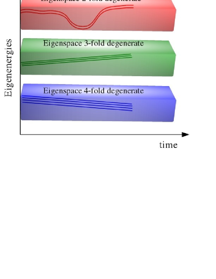
Figure 1: (Color online) Example of spectral time evolution. For DAT and DAPT be meaningful, each eigenspace $\mathcal{H}_{n}$ can have an arbitrary number of fixed degeneracies, but there must always be a gap, constant or not, between different eigenspaces. In DAA, no transitions occur between eigenspaces while within each eigenspace the system acquires the non-abelian WZ phase.

For the sake of comparison, we state DAT in a form that resembles the standard way of presenting AT for non-degenerate systems, namely, when one starts at a given eigenstate of the system (or in a given eigenspace in the degenerate scenario). Assuming, without loss of generality, that the system begins at the ground eigenspace $|\mathbf{0}(0)\rangle$, DAT reads:

If a system’s Hamiltonian $\mathbf{H}(t)$ changes slowly during the course of time, say from $t=0$ to $t=T$, and the system is prepared at the ground eigenspace of $\mathbf{H}(t)$ at $t=0$, then the system evolves according to $|\mathbf{\Psi}^{(0)}(t)\rangle=\mathrm{e}^{-\mathrm{i}\omega_{0}(t)}\mathcal{T}\exp\left(\int_{0}^{t}\mathbf{A}^{nn}(t^{\prime})dt^{\prime}\right)|\mathbf{0}(t)\rangle.$

To avoid any possible misunderstanding it is worth stressing the following: DAA is based on the assumption that the rate of change of $\mathbf{H}(t)$ is slow. Intuitively, the latter notion can be understood as a relation between a characteristic internal time $T_{i}$ of the evolved system (the inverse of its characteristic frequency, for instance) encoded in $\mathbf{H}(t)$ and the total evolution time $T$, related to the time it takes to drive $\mathbf{H}(t)$ throughout the parameter space to its final destination. It is the interplay between these internal and external times that dictates whether DAA is a good approximation for the system time evolution. For a given path in parameter space one can always tune $\mathbf{H}(t)$ to make the system adiabatic, although for some Hamiltonians this will reflect in an evolution time $T$ prohibitively large in a possible experimental implementation. In other words, one can always decrease the rate of change of $\mathbf{H}(t)$ by increasing the time to drive $\mathbf{H}(t)$ to its final configuration in parameter space. This state of affairs, although intuitive, is not satisfactory from a mathematical standpoint since it provides no quantitative notion of slowness. This lack of precise meaning of slow is a main source of controversy. By using DAPT Rig10 , a generalization of APT Rig08 , we can give a precise meaning to this notion of slowness, which is crucial for the derivation of the necessary and sufficient conditions for the validity of DAT.

Therefore, before we state and prove the necessary and sufficient conditions for the validity of DAT, we need first to present DAPT in its full generality and details. DAPT is the tool we need to continue the discussion about DAT and also the correct way to obtain higher order corrections to DAA. Moreover, as we will see, the geometric WZ phase and DAA will appear naturally as the zeroth order term of DAPT.

V Degenerate adiabatic perturbation theory

V.1 The ansatz

An important characteristic of DAPT is its practical utility. As we will see, DAPT can be actually employed to systematically approximate any time-dependent problem whose snapshot Hamiltonian can be efficiently diagonalized. Also, DAPT is, to the best of our knowledge, the first perturbation theory specially designed for degenerate systems about AA. Mathematically, it is a series expansion in terms of the small adiabatic parameter

$$v=1/T,$$

representing the rate of change of $\mathbf{H}(t)$. Moreover, higher order terms of the perturbative series are recursively obtained from their lower order terms.

As extensively discussed for the non-degenerate case Rig08 , the usefulness and success of APT are primarily connected to the choice of the right ansatz for the form of the solution to SE. This can be seen by noticing that the perfect ansatz would factor out the dependence of all terms of order $\mathcal{O}(v^{0})$ and below. In particular, terms $\mathcal{O}(v^{-1})$ and below are the problematic ones when $v\rightarrow 0$ and should be handled with caution. In addition to this, an important insight behind the degenerate ansatz is the recognition that we have non-abelian phases, which are represented by matrices, and a dynamical phase. We have somehow to explore all these facts at the very beginning of the construction of the “vector of vectors” ansatz of DAPT in order to make it work successfully.

Let us write down the ansatz and then explain the quantities appearing in it. We assume that the solution to the time-dependent SE can be written as

$$|\mathbf{\Psi}(s)\rangle=\sum_{p=0}^{\infty}v^{p}|\mathbf{\Psi}^{(p)}(s)\rangle,$$ (11)

where

$$|\mathbf{\Psi}^{(p)}(s)\rangle=\sum_{n=0}\mathrm{e}^{-\frac{\mathrm{i}}{v}\omega_{n}(s)}\mathbf{B}_{n}^{(p)}(s)|\mathbf{n}(s)\rangle$$ (12)

and

$$\mathbf{B}_{n}^{(p)}(s)=\sum_{m=0}\mathrm{e}^{\frac{\mathrm{i}}{v}\omega_{nm}(s)}\mathbf{B}_{mn}^{(p)}(s).$$ (13)

Here $\omega_{nm}(s)=\omega_{n}(s)-\omega_{m}(s)$, $|\mathbf{\Psi}(s)\rangle$ and $|\mathbf{\Psi}^{(p)}(s)\rangle$ are column vectors of dimension $d_{\sf max}=\max_{n}\{d_{n}\}$, while $\mathbf{B}_{n}^{(p)}(s)$ and $\mathbf{B}_{mn}^{(p)}(s)$ are matrices with dimensions $d_{n}\times d_{n}$ and $d_{m}\times d_{n}$, with $d_{n}$ and $d_{m}$ being the level of degeneracy of eigenspaces $\mathcal{H}_{n}$ and $\mathcal{H}_{m}$. We call each element of the vectors and matrices as $[\mathbf{|\Psi}(s)\rangle]_{g_{n},0}=[\mathbf{|\Psi}(s)\rangle]_{g_{n}}$, $[\mathbf{B}_{mn}^{(p)}(s)]_{h_{m}g_{n}}$ and $[\mathbf{B}_{n}^{(p)}(s)]_{h_{n}g_{n}}.$

Note that we are now working with the rescaled time $s=vt$, $s\in[0,1]$ for $t\in[0,T]$. This is crucial to correctly identify the order $v$ of each term appearing in the perturbative series expansion. In the rescaled time the dynamical phase is

$$\omega_{n}(s)=\frac{1}{\hbar}\int_{0}^{s}E_{n}(s^{\prime})ds^{\prime}.$$ (14)

As we said in Sec. II, when we write $E_{n}(s)$ we mean that the function $E_{n}(t)$, or any other function of $t$, is written changing every $t$ by $s/v$. Hence, for example, $E_{n}(t)=at^{3}$ gives $E_{n}(s)=as^{3}/v^{3}$.

Equation (11) tells us that the solution to SE is expressed as a series expansion in the perturbative parameter $v$, with each order given by Eq. (12). Had we stopped at Eq. (12) we would have arrived at a deadlock after inserting the ansatz into SE. In order to make progress and get a recursive relation that gives order $p+1$ coefficient as function of order $p$, Eq. (13) is of utmost importance. Putting all these pieces together the ansatz can be written as

$$\mathbf{|\Psi}(s)\rangle=\sum_{n,m=0}\sum_{p=0}^{\infty}v^{p}\mathrm{e}^{-\frac{\mathrm{i}}{v}\omega_{m}(s)}\mathbf{B}_{mn}^{(p)}(s)\mathbf{|n}(s)\rangle.$$ (15)

Before we proceed, it is important to explain the physical meaning of the small parameter $v=1/T$, whose choice is related to the “velocity” or rate at which $\mathbf{H}(s)$ changes with time. DAPT is best suited for a system in which $\mathbf{H}(s)=\mathbf{H}(\mathbf{r}(s))$ goes from an initial configuration at $s=0$ to a final one at $s=t/T=1$. Its change is driven by the evolution of $\mathbf{r}(s)$ throughout the parameter space, which can be, for instance, a varying external field or an internal coupling constant. The choice of $v$, or equivalently the total time of the experiment $T$, making DAPT convergent depends on how fast or slow $\mathbf{r}(s)$ changes with time. It may happen that DAPT does not converge for a particular combination of the values of the changing rate for $\mathbf{r}(s)$ and the total time $T$ employed to drive the system to the desired configuration in the parameter space. This fact simply implies that AA is not a good approximation for the system’s whole evolution. However, by properly slowing down how $\mathbf{r}(s)$ evolves to its final desired configuration, which subsequently increases the duration $T$ of the experiment, one can make DAPT converge and guarantee AA to be a good description to the system’s whole evolution from $t=0$ to $t=T$. More details about the meaning of $v$ are given when we apply DAPT to several examples in Secs. VII and VIII.

V.2 Initial conditions

In addition to the ansatz that correctly highlights each order $v$ and factors out the dynamical phase, where terms $\mathcal{O}(1/v)$ and below are present, DAPT can only be realized if the initial conditions of the system are taken into account. This is a characteristic of DAPT that differentiates it from all standard perturbation theories, where initial conditions only play a secondary role. Here, however, initial conditions play a central role. When properly handled it introduces additional terms to the perturbation series, without which DAPT fails.

The initial conditions and constraints imposed on the ansatz must satisfy:

• The zeroth order of DAPT ($p=0$) must be such that no transitions between different eigenspaces occur.

• For $p\geq 1$ we must have $\mathbf{|\Psi}^{(p)}(0)\rangle=0$.

Condition (i) implies

$$\mathbf{B}_{n}^{(0)}(s)=b_{n}(0)\mathbf{U}^{n}(s)\Longrightarrow\mathbf{B}_{mn}^{(0)}(s)=b_{n}(0)\mathbf{U}^{n}(s)\delta_{nm},$$ (16)

which leads to (cf. Eq. (4))

$$\mathbf{|\Psi}^{(0)}(s)\rangle=\sum_{n=0}\mathrm{e}^{-\frac{\mathrm{i}}{v}\omega_{n}(s)}b_{n}(0)\mathbf{U}^{n}(s)\mathbf{|n}(s)\rangle,$$ (17)

where we assume nothing about $\mathbf{U}^{n}(s)$ but the fact that it is a unitary matrix at $s=0$. Also, at $s=0$ we recover the initial wave function (3). Condition (ii) in turn implies for $p\geq 1$,

$$\mathbf{B}_{n}^{(p)}(0)=0\Longrightarrow\mathbf{B}_{nn}^{(p)}(0)=-\mathop{\sum_{m=0}}_{m\neq n}\mathbf{B}_{mn}^{(p)}(0).$$ (18)

V.3 The recursive equations

In order to get recursive relations for the matrices $\mathbf{B}_{mn}^{(p)}(s)$ we must work with the transposed ansatz,

$$\mathbf{|\Psi}(s)\rangle^{T}=\sum_{n,m=0}\sum_{p=0}^{\infty}v^{p}\mathrm{e}^{-\frac{\mathrm{i}}{v}\omega_{m}(s)}\mathbf{|n}(s)\rangle^{T}\mathbf{B}_{mn}^{(p)}(s)^{T}$$ (19)

and the transposed SE

$$\mathrm{i}\hbar v\frac{\mathrm{d}}{\mathrm{d}s}\mathbf{|\Psi}(s)\rangle^{T}=\mathbf{H}(s)\mathbf{|\Psi}(s)\rangle^{T}.$$ (20)

Inserting Eq. (19) into Eq. (20) we get

$$\sum_{n,m=0}\sum_{p=0}^{\infty} v^{p} \mathrm{e}^{-\frac{\mathrm{i}}{v}\omega_{m}(s)}\left(\frac{\mathrm{i}}{\hbar v}\Delta_{nm}(s)\mathbf{|n}(s)\rangle^{T}\mathbf{B}_{mn}^{(p)}(s)^{T}\right.$$

$$+ \left.|\dot{\mathbf{n}}(s)\rangle^{T}\mathbf{B}_{mn}^{(p)}(s)^{T}+\mathbf{|n}(s)\rangle^{T}\dot{\mathbf{B}}_{mn}^{(p)}(s)^{T}\right)=0,$$

where

$$\Delta_{nm}(s)=E_{n}(s)-E_{m}(s).$$ (22)

Now, if we left multiply Eq. (LABEL:vector1) by the column vector of bras $\langle\mathbf{k}(s)|^{T}$ we get after using $\langle\mathbf{k}(s)|^{T}|\mathbf{n}(s)\rangle^{T}=\delta_{kn}\mathds{1}$,

$$\sum_{m=0}\sum_{p=0}^{\infty} v^{p} \mathrm{e}^{-\frac{\mathrm{i}}{v}\omega_{m}(s)}\left(\frac{\mathrm{i}}{\hbar v}\Delta_{km}(s)\mathbf{B}_{mk}^{(p)}(s)^{T}+\dot{\mathbf{B}}_{mk}^{(p)}(s)^{T}\right.$$ (23)

$$+ \left.\sum_{n=0}\mathbf{M}^{nk}(s)^{T}\mathbf{B}_{mn}^{(p)}(s)^{T}\right)=0.$$

The first term $\sum_{m}\sum_{p}v^{p}\mathrm{e}^{-\frac{\mathrm{i}}{v}\omega_{m}(s)}\mathrm{i}\Delta_{km}(s)\mathbf{B}_{mk}^{(p)}(s)^{T}/\hbar v$ in Eq. (23) can be cast as follows if we explicitly isolate the $p=0$ term,

$$\sum_{m=0}\sum_{p=0}^{\infty} v^{p} \mathrm{e}^{-\frac{\mathrm{i}}{v}\omega_{m}(s)}\frac{\mathrm{i}}{\hbar}\Delta_{km}(s)\mathbf{B}_{mk}^{(p+1)}(s)^{T}$$ (24)

$$+ \sum_{m=0}\mathrm{e}^{-\frac{\mathrm{i}}{v}\omega_{m}(s)}\frac{\mathrm{i}}{\hbar v}\Delta_{km}(s)\mathbf{B}_{mk}^{(0)}(s)^{T}.$$

Employing the initial condition, Eq. (16), we readily see that the last sum in (24) is zero and SE is satisfied if the remaining terms multiplying $v^{p}\mathrm{e}^{-\frac{\mathrm{i}}{v}\omega_{m}(s)}$ in (23) are zero. This leads to the following recursive condition,

$$\frac{\mathrm{i}}{\hbar}\Delta_{nm}(s)\mathbf{B}_{mn}^{(p+1)}(s)+\dot{\mathbf{B}}_{mn}^{(p)}(s)+\sum_{k=0}\mathbf{B}_{mk}^{(p)}(s)\mathbf{M}^{kn}(s)=0,$$

(25)

where we have swapped the indexes $k\leftrightarrow n$ and taken the transpose. This is the main recursive relation, from which we are able to compute $\mathbf{B}_{mn}^{(p)}(s)$ to all orders in $v=1/T$ and give consistent successive corrections to DAA. As we show in Appendix B, it reduces to the recursive relation obtained in Rig08 for non-degenerate Hamiltonians.

It is worth noting that the initial condition (16) was crucial to cancel the second term of (24), whose limit as $v\rightarrow 0$ diverges. This highlights the importance of the initial conditions on the development of DAPT. In what follows, we will encounter another instance where the other piece of the initial conditions, Eq. (18), becomes relevant.

V.4 The zeroth and first order coefficients

We now explicitly compute $\mathbf{B}_{mn}^{(p)}(s)$ up to first order, i.e., we need to consider the instances where $p=0$ and $p=1$ with either $m=n$ or $m\neq n$.

V.4.1 $p=0$ and $m=n$

In this case Eq. (25) becomes,

$$\dot{\mathbf{B}}_{nn}^{(0)}(s)+\sum_{k=0}\mathbf{B}_{nk}^{(0)}(s)\mathbf{M}^{kn}(s)=0,$$ (26)

and using Eq. (16) we get

$$b_{n}(0)\left(\dot{\mathbf{U}}^{n}(s)+\mathbf{U}^{n}(s)\mathbf{M}^{nn}(s)\right)=0.$$ (27)

Since, in general, $b_{n}(0)\neq 0$ the term inside the parenthesis must necessarily be zero and it becomes $\dot{\mathbf{U}}^{n}(s)=\mathbf{U}^{n}(s)\mathbf{A}^{nn}(s)$, where $\mathbf{M}^{nn}(s)=-\mathbf{A}^{nn}(s)$. The formal solution to that equation is exactly the WZ-phase, Eq. (6). In other words, the WZ-phase naturally appears in the development of DAPT, as anticipated in previous sections. It is the solution to the zeroth order recursive equation supplemented with the correct initial condition.

V.4.2 $p=0$ and $m\neq n$

Now Eq. (25) becomes

$$\frac{\mathrm{i}}{\hbar}\Delta_{nm}(s)\mathbf{B}_{mn}^{(1)}(s)+\sum_{k=0}\mathbf{B}_{mk}^{(0)}(s)\mathbf{M}^{kn}(s)=0,$$ (28)

and using Eq. (16) we get

$$\mathbf{B}^{(1)}_{mn}(s)=\frac{\mathrm{i}\hbar}{\Delta_{nm}(s)}\mathbf{U}^{m}(s)\mathbf{M}^{mn}(s)b_{m}(0),\hskip 7.11317ptm\neq n.$$ (29)

V.4.3 $p=1$ and $m=n$

In this scenario we can write Eq. (25) as follows,

$$\dot{\mathbf{B}}_{nn}^{(1)}(s)+\mathbf{B}_{nn}^{(1)}(s)\mathbf{M}^{nn}(s)+\mathop{\sum_{k=0}}_{k\neq n}\mathbf{B}_{nk}^{(1)}(s)\mathbf{M}^{kn}(s)=0.$$

To solve this equation we make the following change of variables,

$$\mathbf{B}_{nn}^{(1)}(s)=\mathbf{\tilde{B}}_{nn}^{(1)}(s)\mathbf{U}^{n}(s),$$ (30)

which leads to

$$\mathbf{\tilde{B}}_{nn}^{(1)}(s)\left(\dot{\mathbf{U}}^{n}(s)+\mathbf{U}^{n}(s)\mathbf{M}^{nn}(s)\right)+\mathbf{\dot{\tilde{B}}}_{nn}^{(1)}(s)\mathbf{U}^{n}(s)$$

$$+\mathop{\sum_{k=0}}_{k\neq n}\mathbf{B}_{nk}^{(1)}(s)\mathbf{M}^{kn}(s)=0.$$

The term inside the parenthesis is zero (WZ-phase), and using the unitarity of $\mathbf{U}^{n}(s)$ we can solve for $\mathbf{\tilde{B}}_{nn}^{(1)}(s)$,

$$\mathbf{\tilde{B}}_{nn}^{(1)}(s)=\mathbf{\tilde{B}}_{nn}^{(1)}(0)-\!\mathop{\sum_{m=0}}_{m\neq n}\!\int_{0}^{s}\!\!\!\mathbf{B}_{nm}^{(1)}(s^{\prime})\mathbf{M}^{mn}(s^{\prime})\!\left(\mathbf{U}^{n}(s^{\prime})\right)^{\dagger}\!\!\mathrm{d}s^{\prime},$$ (31)

where we have changed $k\rightarrow m$. Next we need to express the initial condition (18) in terms of the new variable $\mathbf{\tilde{B}}_{nn}^{(1)}(s)$. Using the unitarity of $\mathbf{U}^{n}(s)$ and Eq. (29) we can write Eq. (18) for $p=1$ as

$$\mathbf{\tilde{B}}_{nn}^{(1)}(0)=-\mathrm{i}\hbar\mathop{\sum_{m=0}}_{m\neq n}\frac{\mathbf{U}^{m}(0)\mathbf{M}^{mn}(0)\left(\mathbf{U}^{n}(0)\right)^{\dagger}}{\Delta_{nm}(0)}b_{m}(0).$$ (32)

Finally, inserting Eqs. (29) and (32) into (31) and the result into (30) we get

$$\mathbf{B}_{nn}^{(1)}(s) = -\mathrm{i}\hbar\mathop{\sum_{m=0}}_{m\neq n}\frac{\mathbf{U}^{m}(0)\mathbf{M}^{mn}(0)\left(\mathbf{U}^{n}(0)\right)^{\dagger}\mathbf{U}^{n}(s)}{\Delta_{nm}(0)}b_{m}(0)$$ (33)

$$+\mathrm{i}\hbar\mathop{\sum_{m=0}}_{m\neq n}\mathbf{J}^{nmn}(s)\mathbf{U}^{n}(s)b_{n}(0),$$

where we define

$$\mathbf{J}^{nmn}(s)=\int_{0}^{s}\!\!\mathrm{d}s^{\prime}\!\!\left(\frac{\mathbf{U}^{n}(s^{\prime})\mathbf{M}^{nm}(s^{\prime})\mathbf{M}^{mn}(s^{\prime})\left(\mathbf{U}^{n}(s^{\prime})\right)^{\dagger}}{\Delta_{nm}(s^{\prime})}\right)\!.$$ (34)

Note that the initial condition (18) is responsible for the first term of Eq. (33) and the second term depends on the history (integration over time) of the evolution of the system. In the Appendix C we show how to obtain the general solution of Eq. (25), i.e., we provide an explicit expression for $\mathbf{B}_{nm}^{(p+1)}(s)$ in terms of $\mathbf{B}_{nm}^{(p)}(s)$.

V.5 The zeroth and first order corrections

With the previous coefficients we are able to write down the zeroth and first order wave functions that approximate the exact solution to SE according to DAPT.

V.5.1 The zeroth order term

The zeroth order term in the expansion is DAA since we have shown that DAPT implies that $\mathbf{U}^{n}(s)$ is the WZ-phase. For $p=0$ if we insert Eq. (16) into (15) we get

$$\mathbf{|\Psi}^{(0)}(s)\rangle=\sum_{n=0}\mathrm{e}^{-\frac{\mathrm{i}}{v}\omega_{n}(s)}b_{n}(0)\mathbf{U}^{n}(s)\mathbf{|n}(s)\rangle.$$ (35)

Starting at the ground state $|0^{0}(0)\rangle$ we must add condition (8) and we obtain

$$\mathbf{|\Psi}^{(0)}(s)\rangle=\mathrm{e}^{-\frac{\mathrm{i}}{v}\omega_{0}(s)}\mathbf{U}^{0}(s)\mathbf{|0}(s)\rangle.$$ (36)

The first element of the vector above expresses the zeroth order term for the initial condition $|0^{0}(0)\rangle$ as,

$$[\mathbf{|\Psi}^{(0)}(s)\rangle]_{0} = |\Psi^{(0)}(s)\rangle$$ (37)

$$= \mathrm{e}^{-\frac{\mathrm{i}}{v}\omega_{0}(s)}[\mathbf{U}^{0}(s)\mathbf{|0}(s)\rangle]_{0}$$

$$= \mathrm{e}^{-\frac{\mathrm{i}}{v}\omega_{0}(s)}\sum_{g_{0}=0}[\mathbf{U}^{0}(s)]_{0g_{0}}[\mathbf{|0}(s)\rangle]_{g_{0}0}$$

$$= \mathrm{e}^{-\frac{\mathrm{i}}{v}\omega_{0}(s)}\sum_{g_{0}=0}U^{0}_{0g_{0}}(s)|0^{g_{0}}(s)\rangle.$$

V.5.2 The first order correction

Setting $p=1$ in Eq. (12) we can write it as

$$\mathbf{|\Psi}^{(1)}(s)\rangle = \sum_{n=0}\mathrm{e}^{-\frac{\mathrm{i}}{v}\omega_{n}(s)}\mathbf{B}_{nn}^{(1)}(s)\mathbf{|n}(s)\rangle$$ (38)

$$+\mathop{\sum_{n,m=0}}_{m\neq n}\mathrm{e}^{-\frac{\mathrm{i}}{v}\omega_{m}(s)}\mathbf{B}_{mn}^{(1)}(s)\mathbf{|n}(s)\rangle.$$

Inserting Eqs. (29) and (33) we get

$$|\mathbf{\Psi}^{(1)}(s)\rangle = \mathrm{i}\hbar\mathop{\sum_{n,m=0}}_{m\neq n}\mathrm{e}^{-\frac{\mathrm{i}}{v}\omega_{n}(s)}b_{n}(0)\mathbf{J}^{nmn}(s)\mathbf{U}^{n}(s)\mathbf{|n}(s)\rangle-\mathrm{i}\hbar\mathop{\sum_{n,m=0}}_{m\neq n}\mathrm{e}^{-\frac{\mathrm{i}}{v}\omega_{n}(s)}b_{m}(0)\frac{\mathbf{U}^{m}(0)\mathbf{M}^{mn}(0)\left(\mathbf{U}^{n}(0)\right)^{\dagger}\mathbf{U}^{n}(s)}{\Delta_{nm}(0)}\mathbf{|n}(s)\rangle$$ (39)

$$+\mathrm{i}\hbar\mathop{\sum_{n,m=0}}_{m\neq n}\mathrm{e}^{-\frac{\mathrm{i}}{v}\omega_{m}(s)}b_{m}(0)\frac{\mathbf{U}^{m}(s)\mathbf{M}^{mn}(s)}{\Delta_{nm}(s)}\mathbf{|n}(s)\rangle.$$

Note that $\mathbf{|\Psi}^{(1)}(0)\rangle=0$ whether or not $v\rightarrow 0$, as it should be, and that if we have no degeneracy we recover the results of Rig08 . Beginning at the ground state $|0^{0}(0)\rangle$ we should impose the additional condition (8), which leads to

$$|\mathbf{\Psi}^{(1)}(s)\rangle = \mathrm{i}\hbar\sum_{n=1}\mathrm{e}^{-\frac{\mathrm{i}}{v}\omega_{0}(s)}\mathbf{J}^{0n0}(s)\mathbf{U}^{0}(s)\mathbf{|0}(s)\rangle-\mathrm{i}\hbar\sum_{n=1}\mathrm{e}^{-\frac{\mathrm{i}}{v}\omega_{n}(s)}\frac{\mathbf{U}^{0}(0)\mathbf{M}^{0n}(0)\left(\mathbf{U}^{n}(0)\right)^{\dagger}\mathbf{U}^{n}(s)}{\Delta_{n0}(0)}\mathbf{|n}(s)\rangle$$ (40)

$$+\mathrm{i}\hbar\sum_{n=1}\mathrm{e}^{-\frac{\mathrm{i}}{v}\omega_{0}(s)}\frac{\mathbf{U}^{0}(s)\mathbf{M}^{0n}(s)}{\Delta_{n0}(s)}\mathbf{|n}(s)\rangle.$$

Since the desired solution with the appropriate initial condition ($|0^{0}(0)\rangle$) is the first element of the previous vector, $|\Psi^{(1)}(s)\rangle=[\mathbf{|\Psi}^{(1)}(s)\rangle]_{0}$, we get after reversing to the usual notation

$$|\Psi^{(1)}(s)\rangle = \mathrm{i}\hbar\!\sum_{n=1}\!\mathrm{e}^{-\frac{\mathrm{i}}{v}\omega_{0}(s)}\!\!\sum_{g_{0}=0}\![\mathbf{J}^{0n0}(s)\mathbf{U}^{0}(s)]_{0g_{0}}|0^{g_{0}}(s)\rangle-\mathrm{i}\hbar\!\sum_{n=1}\!\!\mathrm{e}^{-\frac{\mathrm{i}}{v}\omega_{n}(s)}\!\sum_{g_{n}=0}\!\frac{[\mathbf{U}^{0}(0)\mathbf{M}^{0n}(0)\left(\mathbf{U}^{n}(0)\right)^{\dagger}\mathbf{U}^{n}(s)]_{0g_{n}}}{\Delta_{n0}(0)}|n^{g_{n}}(s)\rangle$$ (41)

$$+\mathrm{i}\hbar\sum_{n=1}\mathrm{e}^{-\frac{\mathrm{i}}{v}\omega_{0}(s)}\sum_{g_{n}=0}\frac{[\mathbf{U}^{0}(s)\mathbf{M}^{0n}(s)]_{0g_{n}}}{\Delta_{n0}(s)}|n^{g_{n}}(s)\rangle.$$

It is important to stress, as indicated in Ref. Rig08 for the non-degenerate case, that the first term in the rhs of Eq. (41) is generally missing in standard corrections to AA Tho83 ; Che11 . As we will see, when applying these ideas to an exactly solvable example, this term is also of upmost importance to obtain the correct first order correction to DAA.

VI Conditions for the validity of the adiabatic theorem

Now that we have developed the right tool, namely DAPT, we are able to establish conditions for the validity of DAT, as stated in Sec. IV. Important to assess such conditions is the ansatz (15). Since the highly oscillatory terms of order $\mathcal{O}(1/v)$ and below appear at any order $p$, by properly choosing the small parameter $v$ one can always make DAPT perturbative series converge. Hence, the conditions that make DAPT converge supplemented with the condition that the sum of all higher orders $p\geq 1$ is negligible compared to the zeroth order, are sufficient conditions to guarantee the validity of DAT. Contrariwise, if DAPT converges and the system is said to be well described by DAA, then the sum of all higher order terms must be small when compared to the zeroth order term, showing this condition is necessary too. In other words, if DAPT converges we can furnish rigorous necessary and sufficient conditions for the validity of DAT. However, as we will see in Sec. VI.2, testing for the convergence of DAPT series is not an easy task in general. To overcome this limitation we develop practical necessary and sufficient conditions in the following sections.

The necessary condition given in Sec. VI.1 is a generalization to degenerate systems of the standard quantitative condition recently proved to be necessary for non-degenerate Hamiltonians Ton10 . On the other hand, the sufficient condition of Sec. VI.2 relies heavily on DAPT and on the conditions under which higher order terms appearing in the perturbative series of DAPT are negligible when compared to the zeroth order.

VI.1 Necessary condition

To arrive at a necessary condition that is also practical we follow Tong Ton10 and others Ber84 ; Wil84 ; Wil11 and assume that if DAT is valid then the system is well described by DAA and all measurements at any time must indeed be consistent with this assumption. This has a profound implication on the approximate dynamics the system obeys in the following sense Ton10 .

It is not only the fidelity, $|\langle\Psi^{(0)}(t)|\Psi(t)\rangle|$, between the exact solution and DAA that must be close to one for the system’s dynamics to be considered adiabatic. The expectation values of any observable associated to the system should also be close to the ones computed with $|\Psi^{(0)}(t)\rangle$, in particular those related to its geometric phase.

Therefore, for that to be true, we must have that

• DAA approximately satisfies SE.

• The transition probabilities to excited eigenspaces are negligible.

Mathematically, these two assumptions read

• $\mathrm{i}\,\hbar\,|\mathbf{\dot{\Psi}}^{0}(t)\rangle\approx\mathbf{H}(t)|\mathbf{\Psi}^{0}(t)\rangle$ and

• $\left\|\mathbf{\langle n}(t)|^{T}\mathbf{|\Psi}(t)\rangle^{T}\right\|_{\text{max}}\ll 1,\hskip 14.22636ptn\neq 0,$

where $\|\cdot\|_{\sf max}$ is the “max norm”, i.e., the condition $\ll 1$ must be tested against the absolute value of all elements of the matrix above (the bra-column vector and the ket-row vector are combined according to the usual matrix multiplication rule).

From these hypotheses we can derive some lemmas that will be employed in the forthcoming demonstration of the necessary condition.

Since DAA approximately fulfill SE (assumption 1) then we may take it as a good approximation to the exact solution $|\mathbf{\Psi}(t)\rangle$, i.e.,

$$|\mathbf{\Psi}(t)\rangle\approx|\mathbf{\Psi}^{(0)}(t)\rangle\longrightarrow\text{lemma 1}.$$ (42)

Now, using SE, lemma 1, and assumption 1 we get

$$\mathrm{i}\,\hbar\,|\mathbf{\dot{\Psi}}(t)\rangle=\mathbf{H}(t)|\mathbf{\Psi}(t)\rangle\approx\mathbf{H}(t)|\mathbf{\Psi}^{(0)}(t)\rangle\approx\mathrm{i}\,\hbar\,|\mathbf{\dot{\Psi}}^{(0)}(t)\rangle,$$ (43)

leading finally to lemma 2,

$$|\mathbf{\dot{\Psi}}(t)\rangle\approx|\mathbf{\dot{\Psi}}^{(0)}(t)\rangle\longrightarrow\text{lemma 2}.$$ (44)

It is worth noting, as Tong did in the non-degenerate case Ton10 , that (44) is not a trivial result obtained by differentiating both sides of (42). Equation (44) is a consequence of the fact that the state describing the time evolution of the system must satisfy SE, at least approximately, which is what (43) is meant to show.

Our goal next is to prove that the quantitative condition

$$\hbar\left\|\frac{\mathbf{M}^{n0}(t)}{\Delta_{n0}(t)}\right\|_{1}\ll 1,\hskip 14.22636ptn\neq 0,\hskip 14.22636ptt\in[0,T],$$ (45)

is a necessary condition for the validity of DAT. In other words, we want to prove that (45) follows from assumptions 1 and 2 (or equivalently from lemmas 1 and 2 and assumption 2). Here $\left\|A\right\|_{1}=\max\limits_{1\leq j\leq q}\sum_{i=1}^{p}|a_{ij}|$ is the maximum absolute column sum of matrix $\mathbf{A}$ with dimensions $p\times q$.

We start the proof writing the following identity for $n\neq 0$,

$$\mathbf{\langle n}(t)|^{T}\mathbf{|\Psi}(t)\rangle^{T}=\frac{\mathbf{\langle n}(t)|^{T}(\mathbf{H}(t)-E_{0}(t))\mathbf{|\Psi}(t)\rangle^{T}}{\Delta_{n0}(t)}.$$ (46)

Using SE, Eq. (10), we get

$$\mathbf{\langle n}(t)|^{T} | \mathbf{\Psi}(t)\rangle^{T}=\frac{\mathbf{\langle n}(t)|^{T}\left(\mathrm{i}\hbar|\dot{\mathbf{\Psi}}(t)\rangle^{T}-E_{0}(t)\mathbf{|\Psi}(t)\rangle^{T}\right)}{\Delta_{n0}(t)}$$ (47)

$$\approx \frac{\mathbf{\langle n}(t)|^{T}\!\!\left(\mathrm{i}\hbar|\dot{\mathbf{\Psi}}^{(0)}(t)\rangle^{T}-E_{0}(t)\mathbf{|\Psi}^{(0)}(t)\rangle^{T}\right)}{\Delta_{n0}(t)},$$

where the last mathematical step comes from Eqs. (42) and (44). Taking the transpose of (9) we get

$$\mathbf{|\Psi}^{(0)}(t)\rangle^{T}=\mathrm{e}^{-\mathrm{i}\omega_{0}(t)}\mathbf{|0}(t)\rangle^{T}\mathbf{U}^{0}(t)^{T},$$ (48)

which leads to

$$\mathrm{i}\hbar\mathbf{|\dot{\Psi}}^{(0)}\!(t)\! \rangle^{T} =\mathrm{e}^{-\mathrm{i}\omega_{0}(t)}\left(E_{0}(t)\mathbf{|0}(t)\rangle^{T}\mathbf{U}^{0}(t)^{T}\right.$$ (49)

$$+ \left.\mathrm{i}\hbar\mathbf{|0}(t)\rangle^{T}\dot{\mathbf{U}}^{0}(t)^{T}+\mathrm{i}\hbar|\dot{\mathbf{0}}(t)\rangle^{T}\mathbf{U}^{0}(t)^{T}\right).$$

Inserting Eqs. (48) and (49) into (47) and noting that $\mathbf{\langle n}(t)|^{T}\mathbf{|0}(t)\rangle^{T}=\mathbf{0}$ since $n\neq 0$ we obtain

$$\mathbf{\langle n}(t)|^{T}\mathbf{|\Psi}(t)\rangle^{T} \approx \mathrm{i}\hbar\mathrm{e}^{-\mathrm{i}\omega_{0}(t)}\frac{\mathbf{\langle n}(t)|^{T}|\dot{\mathbf{0}}(t)\rangle^{T}\mathbf{U}^{0}(t)^{T}}{\Delta_{n0}(t)}$$ (50)

$$= \mathrm{i}\hbar\mathrm{e}^{-\mathrm{i}\omega_{0}(t)}\frac{\mathbf{\langle n}(t)|^{T}[\mathbf{U}^{0}(t)|\dot{\mathbf{0}}(t)\rangle]^{T}}{\Delta_{n0}(t)}.$$

Taking the max norm of both sides and using assumption $2$ we get the necessary condition

$$\hbar\left\|\frac{\mathbf{\langle n}(t)|^{T}(\mathbf{U}^{0}(t)\mathbf{|\dot{0}}(t)\rangle)^{T}}{\Delta_{n0}(t)}\right\|_{\sf max}\ll 1,\hskip 8.5359ptn\neq 0,\hskip 8.5359ptt\in[0,T].$$ (51)

In order to get a phase-free necessary condition it is convenient to work with (51) in the standard notation. First note that

$$[\mathbf{U}^{0}(t)|\dot{\mathbf{0}}(t)\rangle]^{T}_{j_{0}h_{0}} = [\mathbf{U}^{0}(t)|\dot{\mathbf{0}}(t)\rangle]_{h_{0}j_{0}}$$ (52)

$$= \sum_{g_{0}=0}^{d_{0}-1}[\mathbf{U}^{0}(t)]_{h_{0}g_{0}}(t)[|\dot{\mathbf{0}}(t)\rangle]_{g_{0}j_{0}}$$

$$= \sum_{g_{0}=0}^{d_{0}-1}U_{h_{0}g_{0}}^{0}(t)|\dot{0}^{g_{0}}(t)\rangle,$$

with $j_{0}=0$, i.e., $[|\dot{\mathbf{0}}(t)\rangle]_{g_{0}j_{0}}=[|\dot{\mathbf{0}}(t)\rangle]_{g_{0}}$ is a column vector and $[\mathbf{U}^{0}(t)|\dot{\mathbf{0}}(t)\rangle]^{T}_{j_{0}h_{0}}$ a row vector. Also, with that in mind

$$[\mathbf{\langle n}(t)|^{T}(\mathbf{U}^{0}(t)|\dot{\mathbf{0}}(t)\rangle)^{T}]_{g_{n}h_{0}} = [\mathbf{\langle n}(t)|]^{T}_{g_{n}0}[\mathbf{U}^{0}(t)|\dot{\mathbf{0}}(t)\rangle]^{T}_{0h_{0}}.$$

Using that $[\mathbf{\langle n}(t)|]^{T}_{g_{n}0}=\langle n^{g_{n}}(t)|$ and inserting (52) into (LABEL:almost2) we get

$$[\mathbf{\langle n}(t)|^{T}(\mathbf{U}^{0}(t)\mathbf{|\dot{0}}(t)\rangle)^{T}]_{g_{n}h_{0}} = \langle n^{g_{n}}(t)|\sum_{g_{0}=0}^{d_{0}-1}U_{h_{0}g_{0}}^{0}(t)|\dot{0}^{g_{0}}(t)\rangle$$ (54)

$$= \sum_{g_{0}=0}^{d_{0}-1}U_{h_{0}g_{0}}^{0}(t)\langle n^{g_{n}}(t)|\dot{0}^{g_{0}}(t)\rangle$$

$$= \sum_{g_{0}=0}^{d_{0}-1}U_{h_{0}g_{0}}^{0}(t)M_{g_{n}g_{0}}^{n0}(t).$$

Finally, inserting Eq. (54) into (51) we obtain

$$\hbar\left|\sum_{g_{0}=0}^{d_{0}-1}U_{h_{0}g_{0}}^{0}(t)\frac{M_{g_{n}g_{0}}^{n0}(t)}{\Delta_{n0}(t)}\right|\ll 1,\hskip 8.5359ptn\neq 0,\hskip 8.5359pt\forall g_{n},h_{0}.$$ (55)

Working with Eq. (55) we can finally arrive at (45) by fully exploring the unitarity of $\mathbf{U}^{n}(t)$, i.e., if we use the fact that $\left|U_{h_{0}g_{0}}^{0}(t)\right|\leq 1$ we have

$$\hbar\left|\sum_{g_{0}=0}^{d_{0}-1}U_{h_{0}g_{0}}^{0}(t)\frac{M_{g_{n}g_{0}}^{n0}(t)}{\Delta_{n0}(t)}\right| \leq \hbar\sum_{g_{0}=0}^{d_{0}-1}\left|U_{h_{0}g_{0}}^{0}(t)\frac{M_{g_{n}g_{0}}^{n0}(t)}{\Delta_{n0}(t)}\right|$$ (56)

$$= \hbar\sum_{g_{0}=0}^{d_{0}-1}\left|U_{h_{0}g_{0}}^{0}(t)\right|\left|\frac{M_{g_{n}g_{0}}^{n0}(t)}{\Delta_{n0}(t)}\right|$$

$$\leq \hbar\sum_{g_{0}=0}^{d_{0}-1}\left|\frac{M_{g_{n}g_{0}}^{n0}(t)}{\Delta_{n0}(t)}\right|.$$

Therefore, a stronger necessary condition is

$$\hbar\sum_{g_{0}=0}^{d_{0}-1}\left|\frac{M_{g_{n}g_{0}}^{n0}(t)}{\Delta_{n0}(t)}\right|\ll 1,\hskip 14.22636ptn\neq 0,\hskip 14.22636pt\forall g_{n},\hskip 14.22636ptt\in[0,T],$$ (57)

which is exactly Eq. (45) if we use (7). Note that if Eq. (57) holds, the weaker necessary condition (51) also holds and both reduce to the one in Ton10 when no degeneracy is present. In such a case $\mathbf{M}^{n0}(t)$ is a $1\times 1$ matrix leading to $[\mathbf{M}^{n0}(t)]_{00}=\langle n(t)|\dot{0}(t)\rangle$.

One last remark. If for $n\neq m$ we take the time derivative of the eigenvalue equation $\mathbf{H}(t)|n^{g_{n}}(t)\rangle$ $=$ $E_{n}(t)|n^{g_{n}}(t)\rangle$ and left multiply the result by $\langle m^{h_{m}}(s)|$ we get

$$M^{nm}_{h_{n}g_{m}}(t)=\langle n^{h_{n}}(t)|\mathbf{\dot{H}}(t)|m^{g_{m}}(t)\rangle/\Delta_{mn}(t).$$ (58)

This last expression when inserted into (57) indicates that the necessary condition for the validity of DAT is connected to the square of the gap between eigenspaces and with the rate at which $\mathbf{H}(t)$ changes with time.

VI.2 Sufficient condition

We can write formal rigorous sufficient conditions for the validity of DAT by using the ratio test for ascertaining the convergence of DAPT series. Once the series is guaranteed to converge, additional conditions must be applied to make DAA (DAPT zeroth order) the dominant term in the expansion.

Let us start writing the ansatz (15) in a form better suited to the analysis that follows,

$$|\mathbf{\Psi}(s)\rangle=\sum_{n=0}\sum_{p=0}^{\infty}\mathbf{C}_{n}^{(p)}(s)|\mathbf{n}(s)\rangle,$$ (59)

with

$$\mathbf{C}_{n}^{(p)}(s)=\mathrm{e}^{-\frac{\mathrm{i}}{v}\omega_{n}(s)}v^{p}\mathbf{B}_{n}^{(p)}(s).$$ (60)

Note that for each $n$ we have a series involving the matrix $\mathbf{C}_{n}^{(p)}(s)$, $p=0,1,\ldots,\infty$, where the matrix element $[\mathbf{C}_{n}^{(p)}(s)]_{h_{n}g_{n}}$ is the probability amplitude to order $p$ of the state $|n^{g_{n}}(s)\rangle$ in the expansion (59). As usual, $h_{n}$ handles different initial conditions and, without loss of generality, we stick with $h_{n}=0$, any $n$. For other initial conditions one would take $h_{n}=1,2,\ldots,d_{n}-1$, for any $n$. See Sec. V for details. Therefore, we can apply the ratio test to all matrix elements of $\mathbf{C}_{n}^{(p)}(s)$ and test the convergence of DAPT:

$$\lim_{p\rightarrow\infty}\left|\frac{[\mathbf{C}_{n}^{(p+1)}(s)]_{0g_{n}}}{[\mathbf{C}_{n}^{(p)}(s)]_{0g_{n}}}\right|<1,\hskip 14.22636pt\forall n,g_{n},\hskip 14.22636pts\in[0,1].$$ (61)

If all matrix coefficients satisfy the above condition then DAPT is convergent.

Inserting Eq. (60) into (61) we get

$$\lim_{p\rightarrow\infty}\left|\frac{v[\mathbf{B}_{n}^{(p+1)}(s)]_{0g_{n}}}{[\mathbf{B}_{n}^{(p)}(s)]_{0g_{n}}}\right|<1,\hskip 14.22636pt\forall n,g_{n},\hskip 14.22636pts\in[0,1],$$ (62)

which after using (13) becomes

$$\lim_{p\rightarrow\infty}\left|\frac{v\left[\sum_{m=0}\mathrm{e}^{\frac{\mathrm{i}}{v}\omega_{m}(s)}\mathbf{B}_{mn}^{(p+1)}(s)\right]_{0g_{n}}}{\left[\sum_{m=0}\mathrm{e}^{\frac{\mathrm{i}}{v}\omega_{m}(s)}\mathbf{B}_{mn}^{(p)}(s)\right]_{0g_{n}}}\right|<1.$$ (63)

We can simplify further the previous equation by invoking the comparison test. Let $S_{\alpha}=\sum_{p=0}^{\infty}\alpha_{p}$ and $S_{\beta}=\sum_{p=0}^{\infty}\beta_{p}$ represent two series. Then the comparison test says that if $S_{\beta}$ converges and $|\alpha_{p}|\leq|\beta_{p}|$ then $S_{\alpha}$ also converges. If we define

$$\alpha_{p}=\left[\sum_{m=0}v^{p}\mathrm{e}^{\frac{\mathrm{i}}{v}\omega_{m}(s)}\mathbf{B}_{mn}^{(p)}(s)\right]_{0g_{n}},$$

which is just the element of the series we are testing in Eq. (63), and

$$\beta_{p}=\sum_{m=0}v^{p}\left|\left[\mathbf{B}_{mn}^{(p)}(s)\right]_{0g_{n}}\right|,$$

we clearly see that $|\alpha_{p}|\leq|\beta_{p}|$ and if

$$\lim_{p\rightarrow\infty}\frac{v\sum_{m=0}\left|\left[\mathbf{B}_{mn}^{(p+1)}(s)\right]_{0g_{n}}\right|}{\sum_{m=0}\left|\left[\mathbf{B}_{mn}^{(p)}(s)\right]_{0g_{n}}\right|}<1,\hskip 5.69046pt\forall n,g_{n},\hskip 5.69046pts\in[0,1],$$ (64)

by the comparison test DAPT also converges.

It is interesting to note that the small parameter $v$ is in the numerator. Then, in principle, we can always make the DAPT series converge by choosing a small enough $v$. Of course, in pathological Hamiltonians or in some real world experimental realizations, we may need a really small $v=1/T$, indicating a prohibitively large $T$. This is an indication that this particular Hamiltonian cannot be made to change adiabatically when constrained by the total execution time of the experiment. To solve this problem, we would need to either increase the running time of the experiment or build another device whose description is given by a different Hamiltonian, best suited for the duration of that particular experiment.

The convergence condition (64) plus

$$\left|\sum_{p=0}^{\infty}[\mathbf{C}_{n}^{(p+1)}(s)]_{0g_{n}}\right| \ll \left|[\mathbf{C}_{n}^{(0)}(s)]_{0g_{n}}\right|,$$ (65)

$\forall n,g_{n},\hskip 5.69046pts\in[0,1]$ is what we call the rigorous sufficient condition. Equation (65) guarantees that the sum of all higher orders coefficients are negligible when compared to the zeroth order. This condition is rather intuitive if we remember that from DAPT (see Eq. (15)) $[\mathbf{C}_{n}^{(p)}(s)]_{0g_{n}}=v^{p}\sum_{m=0}\mathrm{e}^{-\frac{\mathrm{i}}{v}\omega_{m}(s)}\left[\mathbf{B}_{mn}^{(p)}(s)\right]_{0g_{n}}$ gives the $p$-th order contribution of state $|n^{g_{n}}(s)\rangle$ to the exact solution.

We can get dynamical phase-free sufficient conditions by noting that

$$\left|\sum_{p=0}^{\infty}[\mathbf{C}_{n}^{(p+1)}(s)]_{0g_{n}}\right| \leq v^{p+1}\sum_{m=0}\left|\left[\mathbf{B}_{mn}^{(p+1)}(s)\right]_{0g_{n}}\right|$$ (66)

and also, by using Eq. (16),

$$\left|[\mathbf{C}_{n}^{(0)}(s)]_{0g_{n}}\right| = \left|b_{n}(0)[\mathbf{U}^{n}(s)]_{0g_{n}}\right|.$$ (67)

Therefore, inserting Eqs. (66) and (67) into (65) we obtain the following stronger sufficient condition footnote1 ,

$$\sum_{p=0}^{\infty}\!\sum_{m=0}\!\!v^{p+1}\!\!\left|\!\left[\mathbf{B}_{mn}^{(p+1)}(s)\right]_{0g_{n}}\!\right| \ll\left|b_{n}(0)[\mathbf{U}^{n}(s)]_{0g_{n}}\right|,$$ (68)

where we must test it for all $n$, $g_{n}$, and $s\in[0,1]$.

The convergence condition (64) is not generally useful in practice since it is extremely difficult to compute the previous limit when $p\rightarrow\infty$. Also, in order to apply (68) we must know all higher order corrections. We can come up, though, with a practical condition of convergence by looking at the ratio for a couple of finite $p$ and truncating (68) at some finite $p$. For example, we can apply Eq. (64) for $p=0,1$, and $2$ with the corresponding truncation of (68). If the previous equations are satisfied by these $p$’s we would have the first order contribution small compared to the zeroth order, the second small compared to the first, and the third order small compared to the second one.

The simplest of all practical tests consists in setting $p=0$ in Eq. (64) and truncating the sum (68) at $p=0$. In this case Eqs. (64) and (68) collapse to the same expression. In other words, Eq. (68) for $p=0$ is what we call the practical sufficient condition and it can be cast as

$$v\sum_{m=0}\left|\left[\mathbf{B}_{mn}^{(1)}(s)\right]_{0g_{n}}\right| \ll |b_{n}(0)|\left|\left[\mathbf{U}^{n}(s)\right]_{0g_{n}}\right|,$$ (69)

$$\hskip 5.69046pt\forall n,g_{n},\hskip 5.69046pts\in[0,1].$$

Assuming the system starts at the ground state $|0^{0}(0)\rangle$ (Eq. 8) we get

$$v\sum_{m=0}\left|\left[\mathbf{B}_{m0}^{(1)}(s)\right]_{0g_{0}}\right|\ll\left|\left[\mathbf{U}^{0}(s)\right]_{0g_{0}}\right|,\hskip 8.5359pt\;\forall g_{0},\hskip 8.5359pts\in[0,1]$$ (70)

and

$$v\sum_{m=0}\left|\left[\mathbf{B}_{mn}^{(1)}(s)\right]_{0g_{n}}\right|\ll 0,\hskip 8.5359pt\forall n\neq 0,\;\forall g_{n},\hskip 8.5359pts\in[0,1].$$ (71)

Note that this last equation, and in particular the zero at the rhs, comes from the fact that $b_{n}(0)=0$ if $n\neq 0$. But the lhs is always positive which means it should be zero. This is too strong a condition since in practice we may have a very tiny contribution from excited states. Also, it may happen that one or more $[\mathbf{U}^{0}(s)]_{0g_{0}}$ are zero. This means that one or more of the eigenstates belonging to the ground eigenspace has, to order zero, a null probability of being populated. Thus, for practical purposes, we should only demand the lhs to be much smaller than the smallest non-null contributions coming from the coefficients of the zeroth order. This guarantees that order zero, and in turn DAA, is the dominant term when compared with the first order correction. Hence, putting all these pieces together the practical sufficient condition looks like

$$v\sum_{m=0}\left|\left[\mathbf{B}_{mn}^{(1)}(s)\right]_{0g_{n}}\right| \ll\min\limits_{\forall g_{0}}\!{}_{+}\left(\left|\left[\mathbf{U}^{0}(s)\right]_{0g_{0}}\right|\right),$$ (72)

$$\hskip 8.5359pt\forall n,g_{n},\hskip 8.5359pts\in[0,1],$$

where $\min\!_{+}$ indicates that the minimum is taken over non-null terms only.

It worth mentioning that we can increase the accuracy of the practical test by repeating the previous calculations for higher orders $p$. The more orders we include the more restrictions we will have and the stronger the sufficient test will be. Here, we are just presenting the simplest set of conditions which, nevertheless, turns out to be very useful as we show in Sec. VII.

Equation (72) is the practical sufficient condition but it still depends on the geometric phase $\mathbf{U}^{n}(s)$ at the lhs. By a similar calculation to the one we did when working with the necessary condition, we can get rid of these unitary matrices though. This procedure gives us a stronger and phase-free practical sufficient test.

Using Eq. (41) we can show that (72) is equivalent to

$$v\hbar\left|\left[\sum_{n=1}\mathbf{J}^{0n0}(s)\mathbf{U}^{0}(s)\right]_{0g_{0}}\right|\ll\min\limits_{\forall g_{0}}\!{}_{+}\left(\left|\left[\mathbf{U}^{0}(s)\right]_{0g_{0}}\right|\right)$$ (73)

and

$$\!\!\!\!\!\frac{v\hbar}{|\Delta_{n0}(0)|}\left(\left|\left[\mathbf{U}^{0}(s)\mathbf{M}^{0n}(s)\right]_{0g_{n}}\right|\right.\left.+\left|\left[\mathbf{U}^{0}(0)\mathbf{M}^{0n}(0)\left(\mathbf{U}^{n}(0)\right)^{\dagger}\mathbf{U}^{n}(s)\right]_{0g_{n}}\right|\right)\ll\min\limits_{\forall g_{0}}\!{}_{+}\left(\left|\left[\mathbf{U}^{0}(s)\right]_{0g_{0}}\right|\right),\hskip 1.42271pt\forall n\neq 0,\;\forall g_{n},$$ (74)

where we used $|a-e^{i\varphi}b|\leq|a|+|b|$ to arrive at the last inequality. Employing the Schwarz inequality we can simplify further the previous two equations. Let us start with the lhs of the first one,

$$\left|\left[\sum_{n=1}\mathbf{J}^{0n0}(s)\mathbf{U}^{0}(s)\right]_{0g_{0}}\right| \leq \sum_{n=1}\left|\left[\mathbf{J}^{0n0}(s)\mathbf{U}^{0}(s)\right]_{0g_{0}}\right|=\sum_{n=1}\left|\sum_{j_{0}=0}^{d_{0}-1}\left[\mathbf{J}^{0n0}(s)\right]_{0j_{0}}\left[\mathbf{U}^{0}(s)\right]_{j_{0}g_{0}}\right|$$ (75)

$$\leq \sum_{n=1}\sum_{j_{0}=0}^{d_{0}-1}\left|\left[\mathbf{J}^{0n0}(s)\right]_{0j_{0}}\right|\left|\left[\mathbf{U}^{0}(s)\right]_{j_{0}g_{0}}\right|\leq\sum_{n=1}\sum_{j_{0}=0}^{d_{0}-1}\left|\left[\mathbf{J}^{0n0}(s)\right]_{0j_{0}}\right|,$$

where the last inequality comes from the fact that $\|\mathbf{U}^{0}(s)\|_{\sf max}\leq 1$. We can further simplify the above equation looking at $\mathbf{J}^{0n0}(s)$ as given in Eq. (34). Working with the matrix element $[\mathbf{J}^{0n0}(s)]_{0j_{0}}$ we have

$$|[\mathbf{J}^{0n0}(s)]_{0j_{0}}| = \left|\int_{0}^{s}\mathrm{d}s^{\prime}\left(\frac{[\mathbf{U}^{0}(s^{\prime})\mathbf{M}^{0n}(s^{\prime})\mathbf{M}^{n0}(s^{\prime})\left(\mathbf{U}^{0}(s^{\prime})\right)^{\dagger}]_{0j_{0}}}{\Delta_{0n}(s^{\prime})}\right)\right|\leq\int_{0}^{s}\mathrm{d}s^{\prime}\left(\frac{\left|[\mathbf{U}^{0}(s^{\prime})\mathbf{M}^{0n}(s^{\prime})\mathbf{M}^{n0}(s^{\prime})\left(\mathbf{U}^{0}(s^{\prime})\right)^{\dagger}]_{0j_{0}}\right|}{|\Delta_{0n}(s^{\prime})|}\right)$$ (76)

$$= \int_{0}^{s}\mathrm{d}s^{\prime}\left(\frac{\sum_{k_{0},l_{n},i_{0}=0}^{d_{0}-1}|[\mathbf{U}^{0}(s^{\prime})]_{0k_{0}}[\mathbf{M}^{0n}(s^{\prime})]_{k_{0}l_{n}}[\mathbf{M}^{n0}(s^{\prime})]_{l_{n}i_{0}}[\left(\mathbf{U}^{0}(s^{\prime})\right)^{\dagger}]_{i_{0}j_{0}}|}{|\Delta_{0n}(s^{\prime})|}\right)$$

$$\leq \int_{0}^{s}\mathrm{d}s^{\prime}\left(\frac{\sum_{k_{0},l_{n},i_{0}=0}^{d_{0}-1}|[\mathbf{M}^{0n}(s^{\prime})]_{k_{0}l_{n}}[\mathbf{M}^{n0}(s^{\prime})]_{l_{n}i_{0}}|}{|\Delta_{0n}(s^{\prime})|}\right)=\int_{0}^{s}\!\!\mathrm{d}s^{\prime}\!\left(\frac{\sum_{k_{0},i_{0}=0}^{d_{0}-1}|[\mathbf{M}^{0n}(s^{\prime})(\mathbf{M}^{0n}(s^{\prime}))^{\dagger}]_{k_{0}i_{0}}|}{|\Delta_{0n}(s^{\prime})|}\right)\!,$$

in which the last equation comes from the fact that $[\mathbf{M}^{nm}(s)]^{\dagger}=-[\mathbf{M}^{mn}(s)].$ Returning to (75) with the aid of (76) we get after noting that its rhs does not depend on $j_{0}$,

$$\left|\left[\sum_{n=1}\mathbf{J}^{0n0}(s)\mathbf{U}^{0}(s)\right]_{0g_{0}}\right|\leq\sum_{n=1}\sum_{j_{0}=0}^{d_{0}-1}\left|\left[\mathbf{J}^{0n0}(s)\right]_{0j_{0}}\right|=d_{0}\int_{0}^{s}\mathrm{d}s^{\prime}\sum_{n=1}\left(\frac{\sum_{k_{0},i_{0}=0}^{d_{0}-1}|[\mathbf{M}^{0n}(s^{\prime})(\mathbf{M}^{0n}(s^{\prime}))^{\dagger}]_{k_{0}i_{0}}|}{|\Delta_{0n}(s^{\prime})|}\right).$$ (77)

Hence the first piece of our practical sufficient condition, Eq. (73), becomes

$$v\hbar d_{0}\int_{0}^{s}\mathrm{d}s^{\prime}\sum_{n=1}\left(\frac{\sum_{k_{0},i_{0}=0}^{d_{0}-1}|[\mathbf{M}^{0n}(s^{\prime})(\mathbf{M}^{0n}(s^{\prime}))^{\dagger}]_{k_{0}i_{0}}|}{|\Delta_{0n}(s^{\prime})|}\right)\ll\min\limits_{\forall g_{0}}\!{}_{+}\left(\left|\left[\mathbf{U}^{0}(s)\right]_{0g_{0}}\right|\right),\hskip 8.5359pts\in[0,1].$$ (78)

For the the second piece of the practical sufficient condition, Eq. (74), it straightforwardly follows that

$$\left|\left[\mathbf{U}^{0}(s)\mathbf{M}^{0n}(s)\right]_{0g_{n}}\right|\leq\sum_{k_{0}=0}^{d_{0}-1}\left|[\mathbf{U}^{0}(s)]_{0k_{0}}[\mathbf{M}^{0n}(s)]_{k_{0}g_{n}}\right|\leq\sum_{k_{0}=0}^{d_{0}-1}\left|[\mathbf{M}^{0n}(s)]_{k_{0}g_{n}}\right|$$ (79)

and

$$\left|\left[\mathbf{U}^{0}(0)\mathbf{M}^{0n}(0)\left(\mathbf{U}^{n}(0)\right)^{\dagger}\mathbf{U}^{n}(s)\right]_{0g_{n}}\right| \leq \sum_{k_{0},l_{n},i_{n}=0}^{d_{0}-1,d_{n}-1}\left|[\mathbf{U}^{0}(0)]_{0k_{0}}[\mathbf{M}^{0n}(0)]_{k_{0}l_{n}}[\left(\mathbf{U}^{n}(0)\right)^{\dagger}]_{l_{n}i_{n}}[\mathbf{U}^{n}(s)]_{i_{n}g_{n}}\right|$$ (80)

$$\leq d_{n}\sum_{k_{0},l_{n}=0}^{d_{0}-1,d_{n}-1}\left|[\mathbf{M}^{0n}(0)]_{k_{0}l_{n}}\right|.$$

Using Eqs. (79) and (80), Eq. (74) becomes

$$\!\!\!\!\frac{v\hbar}{|\Delta_{n0}(0)|}\left(\sum_{k_{0}=0}^{d_{0}-1}\left|[\mathbf{M}^{0n}(s)]_{k_{0}g_{n}}\right|+d_{n}\sum_{k_{0},l_{n}=0}^{d_{0}-1,d_{n}-1}\left|[\mathbf{M}^{0n}(0)]_{k_{0}l_{n}}\right|\right) \ll \min\limits_{\forall g_{0}}\!{}_{+}\left(\left|\left[\mathbf{U}^{0}(s)\right]_{0g_{0}}\right|\right),\hskip 2.84544pt\forall n\neq 0,\;\forall g_{n},\;s\in[0,1].$$ (81)

It is worth noting that the degeneracy level of the eigenspaces are relevant since in Eq. (78) we have $d_{0}$ and in (81) $d_{n}$ explicitly appearing in those equations. They also depend implicitly on the degeneracy level of the eigenspaces since the sums that remain to be computed will have more or less terms whether we have a higher or lower degree of degeneracy. We should also remark that the “history” of the time evolution of the state (integration over time) is important in the sufficient condition (78) while the history does not show up in the necessary condition.

Finally, the practical sufficient conditions (78) and (81) can be expressed in terms of the real time variable $t$ as,

$$\hbar d_{0}\int_{0}^{t}\mathrm{d}t^{\prime}\sum_{n=1}\left(\frac{\sum_{k_{0},i_{0}=0}^{d_{0}-1}|[\mathbf{M}^{0n}(t^{\prime})(\mathbf{M}^{0n}(t^{\prime}))^{\dagger}]_{k_{0}i_{0}}|}{|\Delta_{0n}(t^{\prime})|}\right)\ll\min\limits_{\forall g_{0}}\!{}_{+}\left(\left|\left[\mathbf{U}^{0}(t)\right]_{0g_{0}}\right|\right),\hskip 14.22636pt\hskip 14.22636ptt\in[0,T].$$ (82)

and

$$\frac{\hbar}{|\Delta_{n0}(0)|}\left(\sum_{k_{0}=0}^{d_{0}-1}\left|[\mathbf{M}^{0n}(t)]_{k_{0}g_{n}}\!\right|+d_{n}\sum_{k_{0},l_{n}=0}^{d_{0}-1,d_{n}-1}\left|[\mathbf{M}^{0n}(0)]_{k_{0}l_{n}}\right|\right) \ll \min\limits_{\forall g_{0}}\!{}_{+}\left(\left|\left[\mathbf{U}^{0}(t)\right]_{0g_{0}}\right|\right),\;\forall n\neq 0,\;\forall g_{n},\;t\in[0,T].$$ (83)

VII An analytical example

An important aspect of any useful perturbation theory is that it should work when applied to simple problems whose exact solutions are known. It is decisive that the zeroth and higher order perturbative corrections exactly match the expansion of the exact solution in terms of the perturbative parameter. Indeed, any error in this matching is an indication that a given perturbation theory is prone to failure when applied to more sophisticated problems. It is our next goal to apply DAPT to an exactly solvable degenerate problem and compare its zeroth and first order terms with the equivalent ones obtained by expanding the exact solution about the perturbative parameter. As we will see, we obtain perfect correspondence between the expansion of the exact solution and DAPT perturbative terms.

In order to test DAPT, and the necessary and sufficient conditions of Sec. VI, we start by presenting for the first time all the details of the calculations that led us to exactly solve Rig10 the time-dependent SE for the degenerate Hamiltonian of Bis89 . This model is the simplest degenerate version of the exactly solvable time-dependent non-degenerate spin-1/2 system subjected to a classical rotating magnetic field about a fixed axis Rab54 .

VII.1 The exact solution

Let us consider a four-level system subjected to a rotating classical magnetic field $\mathbf{B}(t)=B\mathbf{r}(t)$ whose magnitude is constant and given by $B=|\mathbf{B}|$. In spherical coordinates $\mathbf{r}(t)=(\sin\theta\cos\varphi(t),\sin\theta\sin\varphi(t),\cos\theta),$ with $0\leq\theta\leq\pi$ and $0\leq\varphi<2\pi$ being the polar and azimuthal angles, respectively. The Hamiltonian describing the four-level system is Bis89

$$\mathbf{H}(t)=\frac{\hbar}{2}b\,\mathbf{r}(t)\cdot\mathbf{\Gamma},$$ (84)

where $b>0$ is proportional to the field $B$ and $\bm{\Gamma}=(\Gamma_{x},\Gamma_{y},\Gamma_{z})$ are the Dirac matrices $\Gamma_{j}=\sigma_{x}\otimes\sigma_{j}$, $j=x,y,z$. Here $\sigma_{j}$ are the usual Pauli matrices, inducing the following algebra for $\Gamma_{j}$,

$$\{\Gamma_{i},\Gamma_{j}\}=2\delta_{ij}\bm{I}_{4},$$

$$[\Gamma_{i},\Gamma_{j}]=2\mathrm{i}\epsilon_{ijk}\Pi_{k},$$

where $\bm{I}_{4}$ is the identity matrix of dimension four, $\delta_{ij}$ the Kronecker delta, $\epsilon_{ijk}$ the Levi-Civita symbol, and $\Pi_{k}=\bm{I}_{2}\otimes\sigma_{k}$.

Hamiltonian (84) may represent a single four-level particle coupled to a rotating magnetic field with coupling constant $b\hbar/2$ or two interacting spin-1/2 particles since $\Gamma_{j}=\sigma_{x}\otimes\sigma_{j}$. In the latter case we have three types of interactions between the two particles, for $j=1,2,3$, whose coupling constants are proportional to the components of $b\mathbf{r}(t)\hbar/2$. In the basis where $\Pi_{z}$ is diagonal, $\{|\!\!\uparrow\uparrow\rangle,|\!\!\uparrow\downarrow\rangle,|\!\!\downarrow\uparrow\rangle,|\!\!\downarrow\downarrow\rangle\}$, the snapshot eigenvectors of $\mathbf{H}(t)$, Eq. (84), are

$$|0^{0}(t)\rangle\! = \!\frac{1}{\sqrt{2}}\!\left(\mathrm{e}^{-\mathrm{i}\varphi(t)}\sin\theta|\!\!\uparrow\uparrow\rangle\!-\!\cos\theta|\!\!\uparrow\downarrow\rangle\!-\!|\!\!\downarrow\downarrow\rangle\right)\!\!,$$ (85)

$$|0^{1}(t)\rangle\! = \!\frac{1}{\sqrt{2}}\!\left(\cos\theta|\!\!\uparrow\uparrow\rangle+\mathrm{e}^{\mathrm{i}\varphi(t)}\sin\theta|\!\!\uparrow\downarrow\rangle-|\!\!\downarrow\uparrow\rangle\right)\!\!,$$ (86)

$$|1^{0}(t)\rangle\! = \!\frac{1}{\sqrt{2}}\!\left(\mathrm{e}^{-\mathrm{i}\varphi(t)}\sin\theta|\!\!\uparrow\uparrow\rangle\!-\!\cos\theta|\!\!\uparrow\downarrow\rangle\!+\!|\!\!\downarrow\downarrow\rangle\right)\!\!,$$ (87)

$$|1^{1}(t)\rangle\! = \!\frac{1}{\sqrt{2}}\!\left(\cos\theta|\!\!\uparrow\uparrow\rangle+\mathrm{e}^{\mathrm{i}\varphi(t)}\sin\theta|\!\!\uparrow\downarrow\rangle+|\!\!\downarrow\uparrow\rangle\right)\!\!.$$ (88)

If we deal with a two spin-1/2 system we also have, for instance, $|\!\!\uparrow\downarrow\rangle=|\!\uparrow\rangle\otimes|\!\downarrow\rangle$, where $|\!\uparrow\rangle$ and $|\!\downarrow\rangle$ are the eigenstates of $\sigma_{z}$. The first two eigenvectors are degenerate with energy $E_{0}$ while the last two have $E_{1}$,

$$E_{0}=-(\hbar/2)b\hskip 8.5359pt \hskip 8.5359ptE_{1}=(\hbar/2)b,$$ and (89)

resulting in a constant gap between the two eigenspaces, $\Delta_{10}(s)$ $=$ $\hbar b$.

If $\varphi(t)=w\,t$, with $w>0$ being the frequency of the rotating magnetic field, we can solve the time-dependent problem exactly by employing techniques similar to those developed for the single spin-1/2 problem Boh93 ; Rab54 . We first define the rotated state

$$|\tilde{\Psi}(t)\rangle=\mathcal{U}^{\dagger}(t)|\Psi(t)\rangle,$$ (90)

with

$$\mathcal{U}(t)=\mathrm{e}^{-\mathrm{i}\frac{wt}{2}\Pi_{z}}.$$ (91)

Inserting Eq. (90) into the SE one can show that $|\tilde{\Psi}(t)\rangle$ evolves according to (10) with a new Hamiltonian

$$\tilde{\mathbf{H}}=\mathcal{U}^{\dagger}(t)\mathbf{H}(t)\mathcal{U}(t)-\mathrm{i}\hbar\mathcal{U}^{\dagger}(t)\frac{{\rm d}\mathcal{U}(t)}{{\rm d}t}.$$ (92)

Using Eq. (91) and the mathematical identity

$$\Gamma_{x}\cos(wt)+\Gamma_{y}\sin(wt)=\mathcal{U}(t)\Gamma_{x}\mathcal{U}^{\dagger}(t),$$

that results from the fact that $[\Pi_{z},\Gamma_{x}]=\mathrm{i}2\Gamma_{y}$ and $[\Pi_{z},\Gamma_{y}]=-\mathrm{i}2\Gamma_{x}$, one can show that Eq. (92) can be written as

$$\tilde{\mathbf{H}} = \frac{\hbar}{2}\left(b\Gamma_{x}\sin\theta+b\Gamma_{z}\cos\theta-w\Pi_{z}\right).$$ (93)

Since $\tilde{\mathbf{H}}$ is time independent $|\tilde{\Psi}(t)\rangle=\mathrm{e}^{-\mathrm{i}\frac{\tilde{\mathbf{H}}t}{\hbar}}|\tilde{\Psi}(0)\rangle.$ Inverting Eq. (90) and noting that $|\tilde{\Psi}(0)\rangle=|\Psi(0)\rangle$ the solution to the original problem is

$$|\Psi(t)\rangle=\mathrm{e}^{-\mathrm{i}\frac{wt}{2}\Pi_{z}}\mathrm{e}^{-\mathrm{i}\frac{\tilde{\mathbf{H}}t}{\hbar}}|\Psi(0)\rangle.$$ (94)

We need now to rewrite the general solution (94) in terms of the snapshot eigenvectors (85)-(88). For ease of notation, we define the following vectors:

$$\mathbf{w} = w\mathbf{z},$$ (95)

$$\mathbf{b} = b\mathbf{r}(t),$$ (96)

$$\mathbf{\Omega_{\pm}} = \mathbf{w}\pm\mathbf{b},$$ (97)

where $\mathbf{z}$ is the unity vector parallel to the $z$-direction and $\theta$ the angle between $\mathbf{w}$ and $\mathbf{b}$. This gives for the magnitude of $\mathbf{\Omega_{\pm}}$,

$$\Omega^{2}_{\pm}=w^{2}+b^{2}\pm 2wb\cos\theta.$$ (98)

The eigenvalues of $\tilde{\mathbf{H}}$ are

$$\tilde{E}_{1}=-\frac{\hbar}{2}\Omega_{-},\hskip 5.69046pt\tilde{E}_{2}=\frac{\hbar}{2}\Omega_{-},\hskip 5.69046pt\tilde{E}_{3}=-\frac{\hbar}{2}\Omega_{+},\hskip 5.69046pt\tilde{E}_{4}=\frac{\hbar}{2}\Omega_{+}.$$ (99)

Note that the transformed Hamiltonian is no longer degenerate. Its eigenvectors are respectively

$$|\tilde{E}_{1}\rangle\! = \!\frac{\tilde{\Omega}_{+-}}{2\sqrt{\Omega_{-}}}\!\left(\!|\!\!\uparrow\uparrow\rangle-\frac{b\sin\theta}{\tilde{\Omega}_{+-}^{2}}|\!\!\uparrow\downarrow\rangle+|\!\!\downarrow\uparrow\rangle-\frac{b\sin\theta}{\tilde{\Omega}_{+-}^{2}}|\!\!\downarrow\downarrow\rangle\!\right)\!\!,$$

$$|\tilde{E}_{2}\rangle\! = \!\frac{\tilde{\Omega}_{-+}}{2\sqrt{\Omega_{-}}}\!\left(\!|\!\!\uparrow\uparrow\rangle+\frac{b\sin\theta}{\tilde{\Omega}_{-+}^{2}}|\!\!\uparrow\downarrow\rangle+|\!\!\downarrow\uparrow\rangle+\frac{b\sin\theta}{\tilde{\Omega}_{-+}^{2}}|\!\!\downarrow\downarrow\rangle\!\right)\!\!,$$

$$|\tilde{E}_{3}\rangle\! = \!\frac{\tilde{\Omega}_{++}}{2\sqrt{\Omega_{+}}}\!\left(\!|\!\!\uparrow\uparrow\rangle+\frac{b\sin\theta}{\tilde{\Omega}_{++}^{2}}|\!\!\uparrow\downarrow\rangle-|\!\!\downarrow\uparrow\rangle-\frac{b\sin\theta}{\tilde{\Omega}_{++}^{2}}|\!\!\downarrow\downarrow\rangle\!\right)\!\!,$$

$$|\tilde{E}_{4}\rangle\! = \!\frac{\tilde{\Omega}_{--}}{2\sqrt{\Omega_{+}}}\!\left(\!|\!\!\uparrow\uparrow\rangle-\frac{b\sin\theta}{\tilde{\Omega}_{--}^{2}}|\!\!\uparrow\downarrow\rangle-|\!\!\downarrow\uparrow\rangle+\frac{b\sin\theta}{\tilde{\Omega}_{--}^{2}}|\!\!\downarrow\downarrow\rangle\!\right)\!\!,$$

where we have defined

$$\tilde{\Omega}_{--}\!=\!\sqrt{\Omega_{+}-w-b\cos\theta}, \tilde{\Omega}_{++}\!=\!\sqrt{\Omega_{+}+w+b\cos\theta},$$

$$\tilde{\Omega}_{-+}\!=\!\sqrt{\Omega_{-}-w+b\cos\theta}, \tilde{\Omega}_{+-}\!=\!\sqrt{\Omega_{-}+w-b\cos\theta}.$$

A general initial state $|\Psi(0)\rangle$ can be written as

$$|\Psi(0)\rangle=\sum_{j=1}^{4}\tilde{a}_{j}(0)|\tilde{E}_{j}\rangle,$$ (100)

with $\tilde{a}_{j}(0)$ given by the initial conditions. Inserting Eq. (100) into (94) we get,

$$|\Psi(t)\rangle=\mathrm{e}^{-\mathrm{i}\frac{wt}{2}\Pi_{z}}\sum_{j=1}^{4}\mathrm{e}^{-\mathrm{i}\frac{\tilde{E}_{j}t}{\hbar}}\tilde{a}_{j}(0)|\tilde{E}_{j}\rangle.$$ (101)

By looking at the definition of $\Pi_{z}$ it is not difficult to see that $\Pi_{z}|\!\!\uparrow\uparrow\rangle=|\!\!\uparrow\uparrow\rangle$, $\Pi_{z}|\!\!\uparrow\downarrow\rangle=-|\!\!\uparrow\downarrow\rangle$, $\Pi_{z}|\!\!\downarrow\uparrow\rangle=|\!\!\downarrow\uparrow\rangle$, and $\Pi_{z}|\!\!\downarrow\downarrow\rangle=-|\!\!\downarrow\downarrow\rangle$. Thus, $|\Psi(t)\rangle$ becomes

$$|\Psi(t)\rangle=\sum_{j=1}^{4}\mathrm{e}^{-\mathrm{i}\frac{\tilde{E}_{j}t}{\hbar}}\tilde{a}_{j}(0)|\tilde{F}_{j}\rangle,$$ (102)

where

$$|\tilde{F}_{1}\rangle = \frac{\mathrm{e}^{-\mathrm{i}\frac{wt}{2}}\tilde{\Omega}_{+-}}{2\sqrt{\Omega_{-}}}\left(|\!\!\uparrow\uparrow\rangle+|\!\!\downarrow\uparrow\rangle-\frac{\mathrm{e}^{\mathrm{i}wt}b\sin\theta}{\tilde{\Omega}_{+-}^{2}}(|\!\!\uparrow\downarrow\rangle+|\!\!\downarrow\downarrow\rangle)\right),$$

$$|\tilde{F}_{2}\rangle = \frac{\mathrm{e}^{-\mathrm{i}\frac{wt}{2}}\tilde{\Omega}_{-+}}{2\sqrt{\Omega_{-}}}\left(|\!\!\uparrow\uparrow\rangle+|\!\!\downarrow\uparrow\rangle+\frac{\mathrm{e}^{\mathrm{i}wt}b\sin\theta}{\tilde{\Omega}_{-+}^{2}}(|\!\!\uparrow\downarrow\rangle+|\!\!\downarrow\downarrow\rangle)\right),$$

$$|\tilde{F}_{3}\rangle = \frac{\mathrm{e}^{-\mathrm{i}\frac{wt}{2}}\tilde{\Omega}_{++}}{2\sqrt{\Omega_{+}}}\left(|\!\!\uparrow\uparrow\rangle-|\!\!\downarrow\uparrow\rangle+\frac{\mathrm{e}^{\mathrm{i}wt}b\sin\theta}{\tilde{\Omega}_{++}^{2}}(|\!\!\uparrow\downarrow\rangle-|\!\!\downarrow\downarrow\rangle)\right),$$

$$|\tilde{F}_{4}\rangle = \frac{\mathrm{e}^{-\mathrm{i}\frac{wt}{2}}\tilde{\Omega}_{--}}{2\sqrt{\Omega_{+}}}\left(|\!\!\uparrow\uparrow\rangle-|\!\!\downarrow\uparrow\rangle-\frac{\mathrm{e}^{\mathrm{i}wt}b\sin\theta}{\tilde{\Omega}_{--}^{2}}(|\!\!\uparrow\downarrow\rangle-|\!\!\downarrow\downarrow\rangle)\right).$$

Since we want to compare the exact solution with DAPT when the system starts at the ground state $|0^{0}(0)\rangle$, we need to determine $\tilde{a}_{j}(0)$ for

$$|\Psi(0)\rangle=|0^{0}(0)\rangle=\frac{1}{\sqrt{2}}\left(\sin\theta|\!\!\uparrow\uparrow\rangle-\cos\theta|\!\!\uparrow\downarrow\rangle-|\!\!\downarrow\downarrow\rangle\right).$$ (103)

Equating Eq. (103) with (102) at $t=0$ we get a linear system of four equations in the variables $\tilde{a}_{j}(0)$, $j=1,\ldots,4$, whose solution is,

$$\tilde{a}_{1}(0) = \frac{(\Omega_{-}-w+b)\tilde{\Omega}_{+-}}{2b\sqrt{2\Omega_{-}}}\cot(\theta/2),$$ (104)

$$\tilde{a}_{2}(0) = -\frac{(\Omega_{-}+w-b)\tilde{\Omega}_{-+}}{2b\sqrt{2\Omega_{-}}}\cot(\theta/2),$$ (105)

$$\tilde{a}_{3}(0) = \frac{(\Omega_{+}-w+b)\tilde{\Omega}_{++}}{2b\sqrt{2\Omega_{+}}}\tan(\theta/2),$$ (106)

$$\tilde{a}_{4}(0) = -\frac{(\Omega_{+}+w-b)\tilde{\Omega}_{--}}{2b\sqrt{2\Omega_{+}}}\tan(\theta/2).$$ (107)

Now that we have the exact solution, with the appropriate initial condition, we just need to re-write it in terms of the snapshot eigenvectors of the original Hamiltonian. In this way, one can straightforwardly compare the expansion of the exact solution up to first order with the perturbative corrections coming from DAPT. Inverting Eqs. (85)-(88) we get

$$|\!\!\uparrow\uparrow\rangle = \frac{1}{\sqrt{2}}\left(\mathrm{e}^{\mathrm{i}wt}\sin\theta|0^{0}(t)\rangle+\cos\theta|0^{1}(t)\rangle\right.$$ (108)

$$+\left.\mathrm{e}^{\mathrm{i}wt}\sin\theta|1^{0}(t)\rangle+\cos\theta|1^{1}(t)\rangle\right),$$

$$|\!\!\uparrow\downarrow\rangle = \frac{1}{\sqrt{2}}\left(-\cos\theta|0^{0}(t)\rangle+\mathrm{e}^{-\mathrm{i}wt}\sin\theta|0^{1}(t)\rangle\right.$$ (109)

$$\left.-\cos\theta|1^{0}(t)\rangle+\mathrm{e}^{-\mathrm{i}wt}\sin\theta|1^{1}(t)\rangle\right),$$

$$|\!\!\downarrow\uparrow\rangle = \frac{1}{\sqrt{2}}\left(-|0^{1}(t)\rangle+|1^{1}(t)\rangle\right),$$ (110)

$$|\!\!\downarrow\downarrow\rangle = \frac{1}{\sqrt{2}}\left(-|0^{0}(t)\rangle+|1^{0}(t)\rangle\right).$$ (111)

Inserting Eqs. (108)-(111) into (102) and using the initial condition (104)-(107) we get after a long but straightforward algebraic manipulation

$$|\Psi(t)\rangle\! = \!\frac{\mathrm{e}^{\mathrm{i}wt/2}}{2}\!\left[\!(1\!+\!\cos\theta)A_{-}(t)\!+\!(1\!-\!\cos\theta)A_{+}(t)\!\right]\!|0^{0}(t)\rangle$$ (112)

$$+\frac{\mathrm{e}^{-\mathrm{i}wt/2}\sin\theta}{2}\left(A_{+}(t)-A_{-}(t)\right)|0^{1}(t)\rangle$$

$$+\frac{\mathrm{e}^{\mathrm{i}wt/2}\sin^{2}\theta}{2}\left(B_{+}(t)+B_{-}(t)\right)|1^{0}(t)\rangle$$

$$+\frac{\mathrm{e}^{-\mathrm{i}wt/2}}{2}\sin\!\theta\!\left[\!(1\!+\!\cos\theta)B_{-}(t)\right.$$

$$\left.-(1\!-\!\cos\!\theta)B_{+}(t)\!\right]\!|1^{1}(t)\rangle,$$

where

$$A_{\pm}(t) = \cos\!\left(\Omega_{\pm}t/2\right)+\mathrm{i}\frac{b\pm w\cos\!\theta}{\Omega_{\pm}}\sin\!\left(\Omega_{\pm}t/2\right)\!,$$ (113)

$$B_{\pm}(t) = \mathrm{i}\frac{w}{\Omega_{\pm}}\sin(\Omega_{\pm}t/2).$$ (114)

VII.2 Expansion of the exact solution

We can write Eq. (112) as

$$|\Psi(t)\rangle = c_{00}(t)|0^{0}(t)\rangle+c_{01}(t)|0^{1}(t)\rangle+c_{10}(t)|1^{0}(t)\rangle$$ (115)

$$+c_{11}(t)|1^{1}(t)\rangle,$$

and our goal is to expand each one of $c_{ij}(t)$ up to first order. As in the non-degenerate case Rig08 we choose $v=w$ for the small perturbative parameter, a natural choice since we have experimental control over the frequency of the rotating field. The smaller $w$ the better is DAA approximation to the exact solution. Also, we must be careful while expanding the exact solution Rig08 since terms $w^{n+1}t$ are of order $w^{n}$ because $t=s/v=s/w$.

VII.2.1 Expansion of $c_{00}(t)$

Looking at Eq. (112) we see that we first need to expand $A_{\pm}(t)$, Eq. (113), up to first order. Using

$$\frac{b\pm w\cos\theta}{\Omega_{\pm}}=1+\mathcal{O}(w^{2})$$

we have

$$A_{\pm}(t)=\mathrm{e}^{\mathrm{i}\frac{\Omega_{\pm}t}{2}}+\mathcal{O}(w^{2}),$$ (116)

which leads to

$$c_{00}(t) = \frac{1}{2}\left[\mathrm{e}^{\mathrm{i}(w+\Omega_{-})t/2}(1+\cos\theta)\right.$$

$$\left.+\mathrm{e}^{\mathrm{i}(w+\Omega_{+})t/2}(1-\cos\theta))\right]+\mathcal{O}(w^{2}).$$

Let us now look at the first exponential. Since

$$w+\Omega_{-}=b+(1-\cos\theta)w+\frac{w^{2}}{2b}\sin^{2}\theta+\mathcal{O}(w^{3})$$

we obtain

$$\mathrm{e}^{\mathrm{i}(w+\Omega_{-})t/2} = \mathrm{e}^{\mathrm{i}bt/2}\mathrm{e}^{\mathrm{i}(1-\cos\theta)wt/2}\left(1+\mathrm{i}\frac{w^{2}t}{4b}\sin^{2}\theta\right)$$ (117)

$$+\mathcal{O}(w^{2}).$$

A similar analysis leads to

$$\mathrm{e}^{\mathrm{i}(w+\Omega_{+})t/2} = \mathrm{e}^{\mathrm{i}bt/2}\mathrm{e}^{\mathrm{i}(1+\cos\theta)wt/2}\left(1+\mathrm{i}\frac{w^{2}t}{4b}\sin^{2}\theta\right)$$ (118)

$$+\mathcal{O}(w^{2}).$$

Combining both results we get after a little algebra

$$c_{00}(t) = \mathrm{e}^{\mathrm{i}\frac{bt}{2}}\mathrm{e}^{\mathrm{i}\frac{wt}{2}}\left(1+\mathrm{i}\frac{w^{2}t}{4b}\sin^{2}\theta\right)\left[\cos\left(\frac{wt}{2}\cos\theta\right)\right.$$ (119)

$$\left.-\mathrm{i}\cos\theta\sin\left(\frac{wt}{2}\cos\theta\right)\right]+\mathcal{O}(w^{2}).$$

VII.2.2 Expansion of $c_{01}(t)$

Similarly,

$$c_{01}(t)=\frac{1}{2}\mathrm{e}^{-\mathrm{i}\frac{wt}{2}}\sin\theta\left(\mathrm{e}^{\mathrm{i}\Omega_{+}t/2}-\mathrm{e}^{\mathrm{i}\Omega_{-}t/2}\right)+\mathcal{O}(w^{2}).$$ (120)

Using Eqs. (117) and (118) we get after some algebra

$$c_{01}(t) = \mathrm{i}\mathrm{e}^{\mathrm{i}\frac{bt}{2}}\mathrm{e}^{-\mathrm{i}\frac{wt}{2}}\left(1+\mathrm{i}\frac{w^{2}t}{4b}\sin^{2}\theta\right)\sin\theta\sin\left(\frac{wt}{2}\cos\theta\right)$$ (121)

$$+\mathcal{O}(w^{2}).$$

VII.2.3 Expansion of $c_{10}(t)$

In this case we need

$$B_{\pm}(t) = \mathrm{i}\frac{w}{b}\sin\left(\frac{\Omega_{\pm}t}{2}\right)+\mathcal{O}(w^{2})$$ (122)

$$= \frac{w}{2b}\mathrm{e}^{\mathrm{i}\frac{\Omega_{\pm}t}{2}}(1-\mathrm{e}^{-\mathrm{i}\Omega_{\pm}t})+\mathcal{O}(w^{2}).$$

Expanding the term inside the parenthesis up to zeroth order gives

$$B_{\pm}(t)=\frac{w}{2b}\mathrm{e}^{\mathrm{i}\frac{\Omega_{\pm}t}{2}}(1-\mathrm{e}^{-\mathrm{i}bt}\mathrm{e}^{\mp\mathrm{i}wt\cos\theta})+\mathcal{O}(w^{2}).$$ (123)

Finally, expanding $\mathrm{e}^{\mathrm{i}\Omega_{\pm}t/2}$ up to zeroth order and using (123) to compute $c_{10}(t)$ (cf. Eq. (112)), we get

$$c_{10}(t) = \mathrm{e}^{\mathrm{i}\frac{bt}{2}}\mathrm{e}^{\mathrm{i}\frac{wt}{2}}\frac{w}{2b}\sin^{2}\theta\cos\left(\frac{wt}{2}\cos\theta\right)\left[1-\mathrm{e}^{-\mathrm{i}bt}\right]$$ (124)

$$+\mathcal{O}(w^{2}).$$

VII.2.4 Expansion of $c_{11}(t)$

Similarly,

$$c_{11}(t) = \mathrm{e}^{\mathrm{i}\frac{bt}{2}}\mathrm{e}^{-\mathrm{i}\frac{wt}{2}}\frac{w}{2b}\sin\theta\!\left[\left(1-\mathrm{e}^{-\mathrm{i}bt}\right)\!\cos\!\left(\!\frac{wt}{2}\cos\theta\!\right)\!\cos\theta\right.$$ (125)

$$\left.-\mathrm{i}\left(1+\mathrm{e}^{-\mathrm{i}bt}\right)\sin\left(\frac{wt}{2}\cos\theta\right)\right]+\mathcal{O}(w^{2}).$$

VII.2.5 $|\Psi(t)\rangle$ up to first order in $v=w$

To first order in $v$, the solution is written as

$$|\Psi(t)\rangle=|\Psi^{(0)}(t)\rangle+v|\Psi^{(1)}(t)\rangle+\mathcal{O}(v^{2}).$$ (126)

Inserting Eqs. (119), (121), (124), and (125) into (115) we obtain

$$\!\!\!\!\!\!\!\!|\Psi^{(0)}(t)\rangle = \mathrm{e}^{\mathrm{i}\frac{bt}{2}}\mathrm{e}^{\mathrm{i}\frac{wt}{2}}\left[\cos\left(\frac{wt}{2}\cos\theta\right)\right.$$

$$- \left.\mathrm{i}\cos\theta\sin\left(\frac{wt}{2}\cos\theta\right)\right]|0^{0}(t)\rangle$$

$$+ \mathrm{i}\mathrm{e}^{\mathrm{i}\frac{bt}{2}}\mathrm{e}^{-\mathrm{i}\frac{wt}{2}}\sin\theta\sin\left(\frac{wt}{2}\cos\theta\right)|0^{1}(t)\rangle,$$

and

$$| \Psi^{(1)}(t)\rangle=\mathrm{i}\mathrm{e}^{\mathrm{i}\frac{bt}{2}}\mathrm{e}^{\mathrm{i}\frac{wt}{2}}\frac{w^{2}t}{4bv}\sin^{2}\theta\left[\cos\left(\frac{wt}{2}\cos\theta\right)\right.$$ (128)

$$- \left.\mathrm{i}\cos\theta\sin\left(\frac{wt}{2}\cos\theta\right)\right]|0^{0}(t)\rangle$$

$$- \mathrm{e}^{\mathrm{i}\frac{bt}{2}}\mathrm{e}^{-\mathrm{i}\frac{wt}{2}}\frac{w^{2}t}{4bv}\sin^{3}\theta\sin\left(\frac{wt}{2}\cos\theta\right)|0^{1}(t)\rangle$$

$$+ \mathrm{e}^{\mathrm{i}\frac{bt}{2}}\mathrm{e}^{\mathrm{i}\frac{wt}{2}}\frac{w}{2bv}\sin^{2}\theta\cos\left(\frac{wt}{2}\cos\theta\right)\left[1-\mathrm{e}^{-\mathrm{i}bt}\right]|1^{0}(t)\rangle$$

$$+ \mathrm{e}^{\mathrm{i}\frac{bt}{2}}\mathrm{e}^{-\mathrm{i}\frac{wt}{2}}\frac{w}{2bv}\sin\theta\left[\left(1-\mathrm{e}^{-\mathrm{i}bt}\right)\cos\theta\cos\left(\frac{wt}{2}\cos\theta\right)\right.$$

$$- \left.\mathrm{i}\left(1+\mathrm{e}^{-\mathrm{i}bt}\right)\sin\left(\frac{wt}{2}\cos\theta\right)\right]|1^{1}(t)\rangle.$$

VII.3 Comparison with DAPT

VII.3.1 Computing the Wilczek-Zee phase

To determine the zeroth and first order contributions in DAPT, we have to perform some previous calculations. We need to explicitly compute the non-abelian geometric WZ-phase since it appears in the corrections coming from DAPT. In particular, we must solve explicitly

$$\dot{\mathbf{U}}^{n}(s)+\mathbf{U}^{n}(s)\mathbf{M}^{nn}(s)=0,$$ (129)

whose formal solution is

$$\mathbf{U}^{n}(s)=\mathbf{U}^{n}(0)\mathcal{T}\exp\left(-\int_{0}^{s}\mathbf{M}^{nn}(s^{\prime})ds^{\prime}\right).$$ (130)

In general, the solution to the coupled differential equations coming from (129) cannot be put into a closed form. Fortunately, for the model we are dealing with such exact closed solution exists.

Since our model has two doubly degenerate eigenvalues, Eq. (129), $\dot{U}^{n}_{h_{n}g_{n}}(s)+\sum_{k_{n}=0}^{1}U^{n}_{h_{n}k_{n}}(s)M^{nn}_{g_{n}k_{n}}(s)=0$, reduces to two sets ($n=0,1$) of four equations ($h_{n}g_{n}=00,01,10,11$):

$$\dot{U}^{n}_{00}(s)+U^{n}_{00}(s)M^{nn}_{00}(s)+U^{n}_{01}(s)M^{nn}_{01}(s) = 0,$$ (131)

$$\dot{U}^{n}_{01}(s)+U^{n}_{00}(s)M^{nn}_{10}(s)+U^{n}_{01}(s)M^{nn}_{11}(s) = 0,$$ (132)

$$\dot{U}^{n}_{10}(s)+U^{n}_{10}(s)M^{nn}_{00}(s)+U^{n}_{11}(s)M^{nn}_{01}(s) = 0,$$ (133)

$$\dot{U}^{n}_{11}(s)+U^{n}_{10}(s)M^{nn}_{10}(s)+U^{n}_{11}(s)M^{nn}_{11}(s) = 0.$$ (134)

Note that the first two equations are not coupled to the last two, which is one of the ingredients for solvability.

Let us start computing the four matrices below (cf. Eq. (7)),

$$\mathbf{M}^{mn}(s)=\left(\begin{array}[]{cccc}M^{nm}_{00}(s)&M^{nm}_{10}(s)\\ M^{nm}_{01}(s)&M^{nm}_{11}(s)\end{array}\right),$$ (135)

with $n,m=0,1$ and $M^{nm}_{h_{n}g_{m}}(s)=\langle n^{h_{n}}(s)|\dot{m}^{g_{m}}(s)\rangle$. An easy calculation using Eqs. (85)-(88) leads to

$$\mathbf{M}^{nm}(s)=\left(\begin{array}[]{cccc}-\frac{\mathrm{i}w}{2v}\sin^{2}\theta&-\frac{\mathrm{i}w}{4v}\sin(2\theta)\mathrm{e}^{-\mathrm{i}\frac{ws}{v}}\\ -\frac{\mathrm{i}w}{4v}\sin(2\theta)\mathrm{e}^{\mathrm{i}\frac{ws}{v}}&\frac{\mathrm{i}w}{2v}\sin^{2}\theta\end{array}\right).$$ (136)

Therefore, since $\mathbf{M}^{00}(s)=\mathbf{M}^{11}(s)$, then $\mathbf{U}^{0}(s)=\mathbf{U}^{1}(s)$, and we have to solve two pairs of coupled equations. Moreover, the first pair of equations, (131) and (132), are formally equivalent to the last one, (133) and (134).

Using Eq. (136) they can be written as follows,

$$\dot{x}(s)-ax(s)+b\mathrm{e}^{\mathrm{i}cs}y(s) = 0,$$ (137)

$$\dot{y}(s)+ay(s)+b\mathrm{e}^{-\mathrm{i}cs}x(s) = 0,$$ (138)

with

$$a=\frac{\mathrm{i}w}{2v}\sin^{2}\theta,\hskip 8.5359pt b=-\frac{\mathrm{i}w}{4v}\sin(2\theta),\hskip 8.5359pt c=\frac{w}{v},$$

and $(x(s),y(s))=(U^{n}_{00}(s),U^{n}_{01}(s))$ or $(x(s),y(s))=(U^{n}_{10}(s),U^{n}_{11}(s))$. There is only one subtle difference between the equations giving either $(U^{n}_{00}(s),U^{n}_{01}(s))$ or $(U^{n}_{10}(s),U^{n}_{11}(s))$. It is the initial condition. Since we adopted $\mathbf{U}^{n}(0)=\mathds{1}$, $\mathds{1}$ being the identity, we have either $(U^{n}_{00}(0),U^{n}_{01}(0))=(1,0)$ or $(U^{n}_{10}(0),U^{n}_{11}(0))=(0,1)$.

In order to solve these coupled differential equations we make the following change of variables

$$\tilde{x}(s)=\mathrm{e}^{-\mathrm{i}cs/2}x(s)\hskip 14.22636pt\mbox{and}\hskip 14.22636pt\tilde{y}(s)=\mathrm{e}^{\mathrm{i}cs/2}y(s),$$

which leads to

$$\dot{\tilde{x}}(s)+(\mathrm{i}c/2-a)\tilde{x}(s)+b\tilde{y}(s) = 0,$$ (139)

$$\dot{\tilde{y}}(s)+(a-\mathrm{i}c/2)\tilde{y}(s)+b\tilde{x}(s) = 0.$$ (140)

Now we have two coupled linear first order differential equations with constant coefficients that can be easily decoupled and solved in closed form. Hence, solving the equations above and returning to the original variables we finally get the WZ-phase,

$$\mathbf{U}^{n}(s) = \left(\begin{array}[]{cccc}U^{n}_{00}(s)&U^{n}_{01}(s)\\ U^{n}_{10}(s)&U^{n}_{11}(s)\end{array}\right),$$ (143)

where for $n=0$ or $1$ we obtain

$$U^{n}_{00}(s) = [U^{n}_{11}(s)]^{*}$$

$$= \mathrm{e}^{\mathrm{i}\frac{ws}{2v}}\!\!\left[\cos\left(\frac{ws}{2v}\cos\theta\right)\right.\left.-\mathrm{i}\cos\theta\sin\left(\frac{ws}{2v}\cos\theta\right)\right]\!,$$

$$U^{n}_{01}(s) = -[U^{n}_{10}(s)]^{*}=\mathrm{i}\mathrm{e}^{-\mathrm{i}\frac{ws}{2v}}\sin\theta\sin\left(\frac{ws}{2v}\cos\theta\right).$$

VII.3.2 Zeroth order correction

For our example, Eq. (37) becomes

$$|\Psi^{(0)}(s)\rangle\! = \mathrm{e}^{-\frac{\mathrm{i}}{v}\omega_{0}(s)}U^{0}_{00}(s)|0^{0}(s)\rangle\!+\!\mathrm{e}^{-\frac{\mathrm{i}}{v}\omega_{0}(s)}U^{0}_{01}(s)|0^{1}(s)\rangle.$$

Using Eq. (143) and remembering that $\omega_{0}(s)=-bs/2=-bvt/2$ and $s=vt$ we get,

$$|\Psi^{(0)}(t)\rangle = \mathrm{e}^{\mathrm{i}\frac{bt}{2}}\mathrm{e}^{\mathrm{i}\frac{wt}{2}}\left[\cos\left(\frac{wt}{2}\cos\theta\right)\right.$$ (144)

$$- \left.\mathrm{i}\cos\theta\sin\left(\frac{wt}{2}\cos\theta\right)\right]|0^{0}(t)\rangle$$

$$+ \mathrm{i}\mathrm{e}^{\mathrm{i}\frac{bt}{2}}\!\mathrm{e}^{-\mathrm{i}\frac{wt}{2}}\!\sin\theta\sin\!\left(\!\frac{wt}{2}\cos\theta\!\right)\!\!|0^{1}(t)\rangle\!,$$

which is identical to the expression obtained by expanding the exact solution up to zeroth order (Eq. (VII.2.5)).

VII.3.3 First order correction

Since we have only two doubly degenerate eigenvalues Eq. (41) becomes

$$| \Psi^{(1)}(s)\rangle=\mathrm{i}\hbar\mathrm{e}^{-\frac{\mathrm{i}}{v}\omega_{0}(s)}[\mathbf{J}^{010}(s)\mathbf{U}^{0}(s)]_{00}|0^{0}(s)\rangle$$ (145)

$$+ \mathrm{i}\hbar\mathrm{e}^{-\frac{\mathrm{i}}{v}\omega_{0}(s)}[\mathbf{J}^{010}(s)\mathbf{U}^{0}(s)]_{01}|0^{1}(s)\rangle$$

$$- \mathrm{i}\hbar\mathrm{e}^{-\frac{\mathrm{i}}{v}\omega_{1}(s)}\frac{[\mathbf{U}^{0}(0)\mathbf{M}^{01}(0)\left(\mathbf{U}^{1}(0)\right)^{\dagger}\mathbf{U}^{1}(s)]_{00}}{\Delta_{10}(0)}|1^{0}(s)\rangle$$

$$- \mathrm{i}\hbar\mathrm{e}^{-\frac{\mathrm{i}}{v}\omega_{1}(s)}\frac{[\mathbf{U}^{0}(0)\mathbf{M}^{01}(0)\left(\mathbf{U}^{1}(0)\right)^{\dagger}\mathbf{U}^{1}(s)]_{01}}{\Delta_{10}(0)}|1^{1}(s)\rangle$$

$$+ \mathrm{i}\hbar\mathrm{e}^{-\frac{\mathrm{i}}{v}\omega_{0}(s)}\frac{[\mathbf{U}^{0}(s)\mathbf{M}^{01}(s)]_{00}}{\Delta_{10}(s)}|1^{0}(s)\rangle$$

$$+ \mathrm{i}\hbar\mathrm{e}^{-\frac{\mathrm{i}}{v}\omega_{0}(s)}\frac{[\mathbf{U}^{0}(s)\mathbf{M}^{01}(s)]_{01}}{\Delta_{10}(s)}|1^{1}(s)\rangle.$$

We can re-write it as follows by noting that our initial conditions imply that $\mathbf{U}^{n}(0)=\mathds{1}$,

$$|\Psi^{(1)}(s)\rangle = \mathrm{i}\hbar\mathrm{e}^{-\frac{\mathrm{i}}{v}\omega_{0}(s)}[\mathbf{J}^{010}(s)\mathbf{U}^{0}(s)]_{00}|0^{0}(s)\rangle$$ (146)

$$+ \mathrm{i}\hbar\mathrm{e}^{-\frac{\mathrm{i}}{v}\omega_{0}(s)}[\mathbf{J}^{010}(s)\mathbf{U}^{0}(s)]_{01}|0^{1}(s)\rangle$$

$$- \mathrm{i}\hbar\left(\mathrm{e}^{-\frac{\mathrm{i}}{v}\omega_{1}(s)}\frac{[\mathbf{M}^{01}(0)\mathbf{U}^{1}(s)]_{00}}{\Delta_{10}(0)}\right.$$

$$- \left.\mathrm{e}^{-\frac{\mathrm{i}}{v}\omega_{0}(s)}\frac{[\mathbf{U}^{0}(s)\mathbf{M}^{01}(s)]_{00}}{\Delta_{10}(s)}\right)|1^{0}(s)\rangle$$

$$- \mathrm{i}\hbar\left(\mathrm{e}^{-\frac{\mathrm{i}}{v}\omega_{1}(s)}\frac{[\mathbf{M}^{01}(0)\mathbf{U}^{1}(s)]_{01}}{\Delta_{10}(0)}\right.$$

$$- \left.\mathrm{e}^{-\frac{\mathrm{i}}{v}\omega_{0}(s)}\frac{[\mathbf{U}^{0}(s)\mathbf{M}^{01}(s)]_{01}}{\Delta_{10}(s)}\right)|1^{1}(s)\rangle,$$

with

$$\mathbf{J}^{010}(s)=\int_{0}^{s}\mathrm{d}s^{\prime}\left(\frac{\mathbf{U}^{0}(s^{\prime})\mathbf{M}^{01}(s^{\prime})\mathbf{M}^{10}(s^{\prime})\left(\mathbf{U}^{0}(s^{\prime})\right)^{\dagger}}{\Delta_{01}(s^{\prime})}\right).$$ (147)

A direct computation gives

$$\mathbf{J}^{010}(s) = \left(\begin{array}[]{cccc}\frac{w^{2}s\sin^{2}\theta}{4v^{2}\hbar b}&0\\ 0&\frac{w^{2}s\sin^{2}\theta}{4v^{2}\hbar b}\end{array}\right).$$ (150)

Putting all these pieces together we get

$$| \Psi^{(1)}(t)\rangle=\mathrm{i}\mathrm{e}^{\mathrm{i}\frac{bt}{2}}\mathrm{e}^{\mathrm{i}\frac{wt}{2}}\frac{w^{2}t}{4bv}\sin^{2}\theta\left[\cos\left(\frac{wt}{2}\cos\theta\right)\right.$$ (151)

$$\left.-\mathrm{i}\cos\theta\sin\left(\frac{wt}{2}\cos\theta\right)\right]|0^{0}(t)\rangle$$

$$-\mathrm{e}^{\mathrm{i}\frac{bt}{2}}\mathrm{e}^{-\mathrm{i}\frac{wt}{2}}\frac{w^{2}t}{4bv}\sin^{3}\theta\sin\left(\frac{wt}{2}\cos\theta\right)|0^{1}(t)\rangle$$

$$+\mathrm{e}^{\mathrm{i}\frac{bt}{2}}\mathrm{e}^{\mathrm{i}\frac{wt}{2}}\frac{w}{2bv}\sin^{2}\theta\cos\left(\frac{wt}{2}\cos\theta\right)\left[1-\mathrm{e}^{-\mathrm{i}bt}\right]|1^{0}(t)\rangle$$

$$+\mathrm{e}^{\mathrm{i}\frac{bt}{2}}\mathrm{e}^{-\mathrm{i}\frac{wt}{2}}\frac{w}{2bv}\sin\theta\left[\left(1-\mathrm{e}^{-\mathrm{i}bt}\right)\cos\theta\cos\left(\frac{wt}{2}\cos\theta\right)\right.$$

$$\left.-\mathrm{i}\left(1+\mathrm{e}^{-\mathrm{i}bt}\right)\sin\left(\frac{wt}{2}\cos\theta\right)\right]|1^{1}(t)\rangle,$$

which is exactly Eq. (128), the first order correction obtained from expanding the exact solution.

It is worth noting that the first order correction terms associated to the degenerate eigenspace $\mathcal{H}^{0}$, i.e., the first two terms of Eq. (151), do not appear in standard approaches trying to correct DAA. In general we only see first order terms related to the excited eigenspaces. This same feature is seen for the non-degenerate case Rig08 , where the corresponding term is also missing Tho83 ; Che11 . However, as the expansion of the exact solution clearly demonstrates, these terms must appear (and they do for DAPT) in any perturbation theory about DAA.

VII.4 The necessary condition

The necessary condition (45) for our example, where we only have two eigenspaces ($n=0,1$), looks like

$$\hbar\left\|\frac{\mathbf{M}^{10}(t)}{\Delta_{10}(t)}\right\|_{1}\ll 1,\hskip 14.22636ptt\in[0,T].$$ (152)

Using Eq. (136) the necessary condition reads

$$\frac{w}{2b}\left|\sin^{2}\theta+\frac{\sin(2\theta)}{2}\right|\ll 1\Longrightarrow\frac{w\sin\theta}{2b}|\sin\theta+\cos\theta|\ll 1.$$ (153)

Note that since the maximum of $|\sin\theta+\cos\theta|$ is $\sqrt{2}$ the condition $\frac{w\sin\theta}{b}\ll 1$ is stronger, i.e., it implies (153). Also, since $\sin\theta$ cannot exceed $1$, $\frac{w}{b}\ll 1$ is even stronger. Our task at this moment is to look at the exact solution, assume that DAA holds, and prove it implies one of the necessary conditions above.

If DAA holds then the absolute values of the coefficients multiplying $|1^{0}(t)\rangle$ and $|1^{1}(t)\rangle$ must be negligible. Therefore, looking at Eq. (112) we must have

$$\frac{\sin^{2}\theta}{2}\left|B_{+}(t)+B_{-}(t)\right|\ll 1,$$ (154)

$$\frac{1}{2}\sin\theta\left|(1+\cos\theta)B_{-}(t)-(1-\cos\theta)B_{+}(t)\right|\ll 1.$$ (155)

Now, using Eq. (114) it implies

$$\frac{w\sin^{2}\theta}{2}\left|\frac{\sin(\Omega_{+}t/2)}{\Omega_{+}}+\frac{\sin(\Omega_{-}t/2)}{\Omega_{-}}\right|\ll 1,$$ (156)

$$\frac{w\!\sin\!\theta}{2}\!\left|\!(1\!+\!\cos\!\theta)\frac{\sin(\Omega_{-}t/2)}{\Omega_{-}}\!-\!(1\!-\!\cos\!\theta)\frac{\sin(\Omega_{+}t/2)}{\Omega_{+}}\!\right|\!\ll\!1.$$

Since we want these coefficients to be very small at all times, let us work with the worst scenario for each one of the inequalities, i.e., when $\sin(\Omega_{\pm}t/2)\approx 1$ for the first one and $\sin(\Omega_{\pm}t/2)\approx\mp 1$ for the second one. This last worst case scenario occurs since $0\leq\theta\leq\pi$ implies $1\pm\cos\theta\geq 0$ and we need a minus sign coming from $\sin(\Omega_{+}t/2)$ to compensate the minus sign before $1-\cos\theta$; all quantities must be positive in the worst case scenario. Hence, those conditions become

$$\frac{w\sin^{2}\theta}{2}\left|\frac{1}{\Omega_{+}}+\frac{1}{\Omega_{-}}\right| \ll 1,$$ (158)

$$\frac{w\sin\theta}{2}\left|(1+\cos\theta)\frac{1}{\Omega_{-}}+(1-\cos\theta)\frac{1}{\Omega_{+}}\right| \ll 1.$$ (159)

Re-writing the last inequality we obtain

$$\frac{w\sin^{2}\theta}{2}\left|\frac{1}{\Omega_{+}}+\frac{1}{\Omega_{-}}\right| \ll 1,$$ (160)

$$\frac{w\sin\theta}{2}\left|\frac{1}{\Omega_{+}}+\frac{1}{\Omega_{-}}+\cos\theta\left(\frac{1}{\Omega_{-}}-\frac{1}{\Omega_{+}}\right)\right| \ll 1.$$ (161)

Actually, these two inequalities are not independent. If the second one is satisfied, so is the first one. To see this note that we can write the first one as

$$\frac{w\sin\theta}{2}\left|\sin\theta\left(\frac{1}{\Omega_{+}}+\frac{1}{\Omega_{-}}\right)\right| \ll 1.$$ (162)

Both inequalities have the same factor multiplying the moduli, $(w\sin\theta)/2$. Hence, if we are able to show that the second absolute value is always greater than the first one, we prove that the second inequality implies the first one. First, we note that we always have $\Omega_{\pm}\geq 0$. Then, looking at the term $\sin\theta\left(1/\Omega_{+}+1/\Omega_{-}\right)$ of the first inequality and $1/\Omega_{+}+1/\Omega_{-}$ of the second, we realize that the latter is always greater than the former since $|\sin\theta|\leq 1$. This means that if we show that the other term of the second inequality, $\cos\theta\left(1/\Omega_{-}-1/\Omega_{+}\right)$, is always positive, we prove our claim. This proof is divided in two parts. We first analyze the case where $\theta\in[0,\pi/2]$ and then the case $\theta\in(\pi/2,\pi]$. These two intervals cover the whole span of the polar angle $\theta$.

Remembering that $\Omega^{2}_{\pm}$ $=$ $w^{2}+b^{2}\pm 2wb\cos\theta$, Eq. (98), we readily see that for $\theta\in[0,\pi/2]$ we must have $\Omega_{+}\geq\Omega_{-}$. This gives $1/\Omega_{-}-1/\Omega_{+}\geq 0$. But in this interval $\cos\theta\geq 0$ implying that $\cos\theta\left(1/\Omega_{-}-1/\Omega_{+}\right)\geq 0$. For $\theta\in(\pi/2,\pi]$, on the other hand, $\Omega_{+}<\Omega_{-}$, which in turn leads to $1/\Omega_{-}-1/\Omega_{+}<0$. Since now $\cos\theta<0$ then $\cos\theta\left(1/\Omega_{-}-1/\Omega_{+}\right)\geq 0$ too, completing our proof.

In other words, we just need to focus on the following inequality

$$\frac{w\sin\theta}{2b}f(\theta) \ll 1,$$ (163)

with

$$f(\theta)=\left|\frac{b}{\Omega_{+}}+\frac{b}{\Omega_{-}}+\cos\theta\left(\frac{b}{\Omega_{-}}-\frac{b}{\Omega_{+}}\right)\right|,$$ (164)

which follows from assuming DAA holds and our task is to show that (163) implies the necessary condition (153).

Note that for any $w,b>0$ (assumed when we solved Hamiltonian (84)) and $\theta\in[0,\pi]$ (polar angle) Eq. (164) has a global minimum at $\theta=\pi/2$. Therefore, $f(\theta)\geq f(\pi/2)=2b/\sqrt{b^{2}+w^{2}}$. When $w<b$ we have,

$$f(\theta)\geq\frac{2b}{\sqrt{b^{2}+w^{2}}}=\frac{2}{\sqrt{1+w^{2}/b^{2}}}\geq\frac{2}{\sqrt{1+1}}=\sqrt{2}.$$

The last inequality results from the fact that $w<b$. With this lower bound the lhs of (163) becomes

$$\frac{w\sin\theta}{2b}f(\theta)\geq\frac{w\sin\theta}{2b}\sqrt{2}\geq\frac{w\sin\theta}{2b}|\sin\theta+\cos\theta|,$$ (165)

where the last inequality is a consequence of $\sqrt{2}$ being the maximum of $|\sin\theta+\cos\theta|$. Equivalently,

$$\frac{w\sin\theta}{2b}|\sin\theta+\cos\theta|\leq\frac{w\sin\theta}{2b}f(\theta).$$ (166)

But the lhs above is just the expression coming from the necessary condition. Hence, since whenever the adiabatic approximation holds $\frac{w\sin\theta}{2b}f(\theta)\ll 1$, we have that the necessary condition is automatically satisfied.

For completeness, let us analyze what happens for $w\geq b$, when it is expected that DAA does not hold since the rotating frequency $w$ of the magnetic field is greater or equal to $b$, i.e., the Hamiltonian changes in a rate ($w$) at least as big as the internal characteristic frequency of the system ($b$). Note also that unless $\theta\approx 0$ the necessary condition cannot be satisfied either (cf. Eq. (153)).

In this case

$$f(\theta)\geq\frac{2b}{\sqrt{b^{2}+w^{2}}}=\frac{2b}{w}\frac{1}{\sqrt{1+b^{2}/w^{2}}}\geq\frac{b}{w}\sqrt{2}.$$

This implies that the lhs of Eq. (163) becomes

$$\frac{w\sin\theta}{2b}f(\theta)>\frac{w\sin\theta}{2b}\frac{b}{w}\sqrt{2}=\sin\theta\frac{\sqrt{2}}{2}\approx\sin\theta.$$ (167)

For not too small $\theta$ we have $\sin\theta\approx 1$ and it is clear that the system is not described by the adiabatic approximation. Indeed, Eq. (167) implies that at least one of the coefficients multiplying the excited states $|1^{0}(t)\rangle$ or $|1^{1}(t)\rangle$ is of order $\sin\theta$.

When in addition to $w\geq b$ we have $\theta\approx 0$, it can be shown that DAA continues to be a bad approximation to the evolution of the system, despite the fact that the fidelity between the exact solution and DAA approaches one and that the necessary condition is satisfied. As shown in Appendix D, if $w\geq b$ and $\theta\approx 0$ the probability to measure the system at the excited state $|1^{1}(t)\rangle$ is of the same order in $\theta$ as that of measuring it in $|0^{1}(t)\rangle$. This clearly indicates that the necessary condition is not a sufficient one. However, the sufficient condition derived in the next section excludes this case as an instance where one can approximate the system’s evolution by DAA.

VII.5 The sufficient condition

For the specific problem we are dealing with the sufficient conditions, Eqs. (82) and (83), become

$$2\hbar\int_{0}^{t}\mathrm{d}t^{\prime}\left(\frac{\sum_{k_{0},i_{0}=0}^{1}|[\mathbf{M}^{01}(t^{\prime})(\mathbf{M}^{01}(t^{\prime}))^{\dagger}]_{k_{0}i_{0}}|}{|\Delta_{01}(t^{\prime})|}\right)\ll\min\limits_{\forall g_{0}}\!{}_{+}\left(\left|\left[\mathbf{U}^{0}(t)\right]_{0g_{0}}\right|\right),\hskip 14.22636ptt\in[0,T],$$ (168)

and

$$\frac{\hbar}{|\Delta_{10}(0)|}\left(\sum_{k_{0}=0}^{1}\left|[\mathbf{M}^{01}(t)]_{k_{0}g_{1}}\right|+2\sum_{k_{0},l_{1}=0}^{1}\left|[\mathbf{M}^{01}(0)]_{k_{0}l_{1}}\right|\right) \ll \min\limits_{\forall g_{0}}\!{}_{+}\left(\left|\left[\mathbf{U}^{0}(t)\right]_{0g_{0}}\right|\right),\;\forall g_{1},\;t\in[0,T].$$ (169)

Note that this last equation encompasses two instances, $g_{1}=0$ and $g_{1}=1$. Let us simplify each one separately.

Using (136) the numerator of Eq. (168) can be written as

$$\sum_{k_{0},i_{0}=0}^{1}|[\mathbf{M}^{01}(t)(\mathbf{M}^{01}(t))^{\dagger}]_{k_{0}i_{0}}|=\frac{w^{2}\sin^{2}\theta}{2}.$$ (170)

Hence, Eq. (168) is simply

$$\frac{w^{2}t}{b}\sin^{2}\theta\ll\min\limits_{\forall g_{0}}\!{}_{+}\left(\left|\left[\mathbf{U}^{0}(t)\right]_{0g_{0}}\right|\right),\hskip 14.22636ptt\in[0,T].$$ (171)

Moving our attention to the other sufficient condition we first note that $\sum_{k_{0}=0}^{1}\left|[\mathbf{M}^{01}(t)]_{k_{0}g_{1}}\right|$ gives the same sum whether $g_{1}=0$ or $g_{1}=1$. In other words, we have only one case to consider. Using Eq. (136) a direct calculation gives

$$\frac{5w}{4b}(|\sin(2\theta)|+2\sin^{2}\theta) \!\ll\! \min\limits_{\forall g_{0}}\!{}_{+}\left(\left|\left[\mathbf{U}^{0}(t)\right]_{0g_{0}}\right|\right),\;t\in[0,T]$$

But since $\theta\in[0,\pi]$ we can write the previous expression as

$$\frac{5w}{2b}\sin\theta(|\cos\theta|+\sin\theta) \!\ll\! \min\limits_{\forall g_{0}}\!{}_{+}\left(\left|\left[\mathbf{U}^{0}(t)\right]_{0g_{0}}\right|\right),\;t\in[0,T].$$

Using the WZ-phase (143) it is not difficult to see that

$$\left|\left[\mathbf{U}^{0}(t)\right]_{00}\right|=\sqrt{1-\sin^{2}\theta\sin^{2}\left(\frac{wt\cos\theta}{2}\right)}$$

and

$$\left|\left[\mathbf{U}^{0}(t)\right]_{01}\right|=\sin\theta\left|\sin\left(\frac{wt\cos\theta}{2}\right)\right|.$$

Furthermore, in this example we chose $v=w=1/T$ which implies that $wt\leq 1$ during the whole evolution. Thus $|\sin(wt\cos(\theta)/2)|\leq\sin(1/2)$ leading to

$$|[\mathbf{U}^{0}(t)]_{00}|\geq|[\mathbf{U}^{0}(t)]_{01}|$$

and to

$$\frac{5w}{2b}\sin\theta(|\cos\theta|+\sin\theta)\geq\frac{w^{2}t}{b}\sin^{2}\theta.$$

With these two inequalities we see that Eqs. (171) and (LABEL:s2) collapse to the following sufficient condition,

$$\frac{5w}{2b} \!\ll\! \frac{\left|\sin\left(\frac{wt\cos\theta}{2}\right)\right|}{|\cos\theta|+\sin\theta},\;\;t\in[0,T].$$ (173)

Notice that for $t\approx 0$ and $\theta\approx\pi/2$ we have $|[\mathbf{U}^{0}(t)]_{01}|\approx 0$ and we need to work with the non-null coefficient $|[\mathbf{U}^{0}(t)]_{00}|$. In this scenario the sufficient condition becomes $5w/(2b)\ll 1$.

First thing we note is that, at least for this example, the sufficient condition is stronger than, and implies, the necessary condition. To see this, take Eq. (LABEL:s2). It is not difficult to see that

$$\frac{5w}{2b}\sin\theta(|\cos\theta|+\sin\theta)\geq\frac{w}{2b}\sin\theta|\cos\theta+\sin\theta|.$$

Hence, if Eq. (LABEL:s2) is satisfied we automatically have

$$\frac{w}{2b}\sin\theta|\cos\theta+\sin\theta|\ll 1,$$

which is exactly the necessary condition, Eq. (153). See also Ref. Yuk09 for an alternative route to establish sufficient conditions in non-degenerate systems, claimed to be general and in some cases also necessary.

Second, if $w\geq b$ we cannot satisfy the sufficient condition (173) irrespective of the value of $\sin\theta$. This is true because the rhs of (173) is never greater than one. Thus, if $w\geq b$ the lhs is always greater than one and the inequality cannot be satisfied at all. This is a very satisfactory restriction that shows the sufficient condition is consistent with the cases where the necessary one fails.

To complete the analysis we just need to show that for $w<b$ the sufficient condition implies DAA. In other words, we must show that the absolute values of the coefficients multiplying $|1^{0}(t)\rangle$ and $|1^{1}(t)\rangle$ are negligible if the sufficient condition holds.

To show that in a clear and straightforward manner we first need to manipulate algebraically those coefficients. Let us call them $C_{|1^{0}(t)\rangle}$ and $C_{|1^{1}(t)\rangle}$. From Eq. (112) and remembering that $\theta\in[0,\pi]$ we have

$$|C_{|1^{0}(t)\rangle}| \!=\! \frac{\sin^{2}\theta}{2}\!\left|B_{+}(t)\!+\!B_{-}(t)\right|\!\leq\!\frac{\sin\theta}{2}\!\left|B_{+}(t)+B_{-}(t)\right|\!,$$

$$|C_{|1^{1}(t)\rangle}| = \frac{\sin\theta}{2}\left|(1+\cos\theta)B_{-}(t)-(1-\cos\theta)B_{+}(t)\right|$$

$$\leq \frac{\sin\theta}{2}\left|(1+\cos\theta)B_{-}(t)+(1-\cos\theta)B_{+}(t)\right|$$

$$= \frac{\sin\theta}{2}\left|B_{+}(t)+B_{-}(t)+\cos\theta(B_{-}(t)-B_{+}(t))\right|.$$

Using Eq. (114) and the maximum value possible for $\sin(\Omega_{\pm}t/2)$ we have

$$|C_{|1^{0}(t)\rangle}| \!\leq\! \frac{w\!\sin\theta}{2b}\!\left|\frac{b}{\Omega_{+}}\!+\!\frac{b}{\Omega_{-}}\right|,$$ (174)

$$|C_{|1^{1}(t)\rangle}| \!\leq\! \frac{w\!\sin\theta}{2b}\!\left|\!\frac{b}{\Omega_{+}}\!+\!\frac{b}{\Omega_{-}}\!+\!|\cos\theta|\!\left(\!\frac{b}{\Omega_{-}}\!+\!\frac{b}{\Omega_{+}}\!\right)\!\right|\!.$$ (175)

It is obvious that the rhs of the last inequality is greater than the rhs of the first one. Hence, if we show that the sufficient conditions imply that the rhs of Eq. (175) is much smaller than one the proof is accomplished.

To this end we write the rhs of Eq. (175) as follows

$${\sf rhs}(\theta) = \frac{w}{2b}(1+|\cos\theta|)\sin\theta\left(\frac{b}{\Omega_{+}}+\frac{b}{\Omega_{-}}\right)$$ (176)

$$\leq \frac{w}{b}\sin\theta\left(\frac{b}{\Omega_{+}}+\frac{b}{\Omega_{-}}\right).$$

But one can show that the function

$$g(\theta)=\sin\theta\left(\frac{b}{\Omega_{+}}+\frac{b}{\Omega_{-}}\right)$$

has a maximum for $\theta\in[0,\pi]$ at $\theta=\pi/2$ given by $g_{\sf max}=2b/\sqrt{b^{2}+w^{2}}.$ Therefore,

$${\sf rhs}(\theta) \leq \frac{w}{b}g_{\sf max}=\frac{2w}{\sqrt{b^{2}+w^{2}}}=\frac{2w}{b}\frac{1}{\sqrt{1+w^{2}/b^{2}}}\leq\frac{2w}{b}.$$

From (173) we can show for $t\in[0,T]$ that

$$\frac{\left|\sin\left(\frac{wt\cos\theta}{2}\right)\right|}{|\cos\theta|+\sin\theta}\leq\sin(1/2)\approx 0.48<1/2,$$

since $wt\leq 1$. Therefore, the sufficient condition (173) and the case where $\theta\approx\pi/2$ reduces to

$$5w/b\ll 1,\;\;t\in[0,T],$$ (177)

which obviously implies $2w/b\ll 1,$ the condition needed to have all coefficients of the excited eigenspace negligible.

VIII Numerical examples

We now want to test DAPT for other degenerate Hamiltonians with and without a constant gap. For that purpose we work with the following Hamiltonian, already written in the rescaled time $s$,

$$\mathbf{H}(s)=\frac{1}{\sqrt{2}}\left(\begin{array}[]{cc}\mathbf{0}&\mathbf{H}_{1}(s)\\ \mathbf{H}_{1}^{\dagger}(s)&\mathbf{0}\end{array}\right),$$ (178)

where

$$\mathbf{H}_{1}(s) = \left(\begin{array}[]{cccc}-E(s)&\mathrm{e}^{-\mathrm{i}\theta(s)}E(s)\\ \mathrm{e}^{\mathrm{i}\theta(s)}E(s)&E(s)\end{array}\right),$$ (181)

$$E(s) = E_{0}+\lambda(s-1/2)^{2},$$ (182)

$$\theta(s) = \theta_{0}+ws^{2}.$$ (183)

Note that for $\lambda=0$ the gap is constant while for $\lambda>0$ it changes quadratically in time achieving its minimum value at $s=1/2$.

Hamiltonian (178) is a doubly degenerate system with eigenvalues given by $-E(s)$ and $E(s)$, and corresponding eigenvectors

$$|0^{0}(s)\rangle\! = \!\frac{1}{2}\!\left(\mathrm{e}^{-\mathrm{i}\theta(s)}|\!\!\uparrow\uparrow\rangle+|\!\!\uparrow\downarrow\rangle-\sqrt{2}|\!\!\downarrow\downarrow\rangle\!\right)\!\!,$$ (184)

$$|0^{1}(s)\rangle\! = \!\frac{1}{2}\!\left(\!|\!\!\uparrow\uparrow\rangle-\mathrm{e}^{\mathrm{i}\theta(s)}|\!\!\uparrow\downarrow\rangle+\sqrt{2}|\!\!\downarrow\uparrow\rangle\!\right)\!\!,$$ (185)

$$|1^{0}(s)\rangle\! = \!\frac{1}{2}\!\left(\mathrm{e}^{-\mathrm{i}\theta(t)}|\!\!\uparrow\uparrow\rangle+|\!\!\uparrow\downarrow\rangle+\sqrt{2}|\!\!\downarrow\downarrow\rangle\!\right)\!\!,$$ (186)

$$|1^{1}(s)\rangle\! = \!\frac{1}{2}\!\left(\!|\!\!\uparrow\uparrow\rangle-\mathrm{e}^{\mathrm{i}\theta(s)}|\!\!\uparrow\downarrow\rangle-\sqrt{2}|\!\!\downarrow\uparrow\rangle\!\right)\!\!.$$ (187)

An arbitrary state in the standard basis

$$|\Psi(s)\rangle=\sum_{i,j=\downarrow,\uparrow}c_{ij}(s)|ij\rangle$$ (188)

when inserted into SE (20) leads to the following set of coupled differential equations,

$$\mathrm{i}\epsilon\dot{c}_{\uparrow\uparrow}(s) = -c_{\downarrow\uparrow}(s)+\mathrm{e}^{-\mathrm{i}\theta(s)}c_{\downarrow\downarrow}(s),$$ (189)

$$\mathrm{i}\epsilon\dot{c}_{\uparrow\downarrow}(s) = \mathrm{e}^{\mathrm{i}\theta(s)}c_{\downarrow\uparrow}(s)+c_{\downarrow\downarrow}(s),$$ (190)

$$\mathrm{i}\epsilon\dot{c}_{\downarrow\uparrow}(s) = -c_{\uparrow\uparrow}(s)+\mathrm{e}^{-\mathrm{i}\theta(s)}c_{\uparrow\downarrow}(s),$$ (191)

$$\mathrm{i}\epsilon\dot{c}_{\downarrow\downarrow}(s) = \mathrm{e}^{\mathrm{i}\theta(s)}c_{\uparrow\uparrow}(s)+c_{\uparrow\downarrow}(s),$$ (192)

where

$$\epsilon(s)=\sqrt{2}\hbar v/E(s).$$ (193)

We assume that the system starts at the ground state $|0^{0}(0)\rangle$ which gives the following initial conditions $c_{\uparrow\uparrow}(0)=\mathrm{e}^{-\mathrm{i}\theta_{0}}/2$, $c_{\uparrow\downarrow}(0)=1/2$, $c_{\downarrow\uparrow}(0)=0$, and $c_{\downarrow\downarrow}(0)=-\sqrt{2}/2$.

To compare the exact time-evolved state with the corrections coming from DAPT it is better to express Eq. (188) in terms of the snapshot eigenvectors (184)-(187),

$$|\Psi(s)\rangle=\sum_{i,j=0,1}d_{ij}(s)|i^{j}(s)\rangle,$$ (194)

where

$$d_{00}(s)=(\mathrm{e}^{\mathrm{i}\theta(s)}c_{\uparrow\uparrow}(s)+c_{\uparrow\downarrow}(s)-\sqrt{2}c_{\downarrow\downarrow}(s))/2,$$ (195)

$$d_{01}(s)=(c_{\uparrow\uparrow}(s)-\mathrm{e}^{-\mathrm{i}\theta(s)}c_{\uparrow\downarrow}(s)+\sqrt{2}c_{\downarrow\uparrow}(s))/2,$$ (196)

$$d_{10}(s)=(\mathrm{e}^{\mathrm{i}\theta(s)}c_{\uparrow\uparrow}(s)+c_{\uparrow\downarrow}(s)+\sqrt{2}c_{\downarrow\downarrow}(s))/2,$$ (197)

$$d_{11}(s)=(c_{\uparrow\uparrow}(s)-\mathrm{e}^{-\mathrm{i}\theta(s)}c_{\uparrow\downarrow}(s)-\sqrt{2}c_{\downarrow\uparrow}(s))/2.$$ (198)

We measure the closeness between the exact solution (194), numerically obtained by solving Eqs. (189)-(192), and the states $|\Psi(s)\rangle_{N_{k}}$, via the infidelity Rig08

$$I_{k}(s)=1-|\langle\Psi(s)|\Psi(s)\rangle_{N_{k}}|^{2}.$$ (199)

Here $|\Psi(s)\rangle_{N_{k}}$ is the normalized state with terms up to order $k$ obtained from DAPT,

$$|\Psi(s)\rangle_{N_{k}}=N_{k}(s)\sum_{p=0}^{k}v^{p}|\Psi^{(p)}(s)\rangle,$$

with $N_{k}(s)$ being a normalization factor, and $0\leq I_{k}(s)\leq 1$. The smaller $I_{k}(s)$ the closer $|\Psi(s)\rangle_{N_{k}}$ is to the exact solution while for $I_{k}(s)=1$ they become orthogonal.

The state $|\Psi^{(p)}(s)\rangle$ is obtained solving the recursive relation (25) with the initial conditions (8), (16), and (18). After that, we pick the first element of the vector (12) leading to the state $|\Psi^{(p)}(s)\rangle$ as given above.

The first case we study is the one with $\lambda=0$, i.e., the case with a constant gap. In contrast to the exactly solvable model of Sec. VII, where we also had a constant gap, now the time dependence of the Hamiltonian is quadratic in $s$.

Building on previous knowledge and similar examples for non-degenerate systems Rig08 we expect that the quality of DAPT will depend on the interplay between the parameter $v$ and the minimum gap between the ground and excited eigenspaces; the smaller the gap the smaller $v$ must be for DAPT to provide meaningful results. Therefore, looking at Eq. (193) we realize that whenever $\epsilon(s)\ll 1$ DAPT is supposed to give accurate results.

This is indeed the case as Figs. 2 and 3 illustrate. For $\epsilon\approx 0.5$ (Fig. 2) we notice that the more orders we include in the perturbation series the better. Also, by just going up to second order in $v$ we already get an excellent description of the exact solution. On the other hand, for $\epsilon\approx 1.4$ (Fig. 3) we observe, as expected, the break down of DAPT.

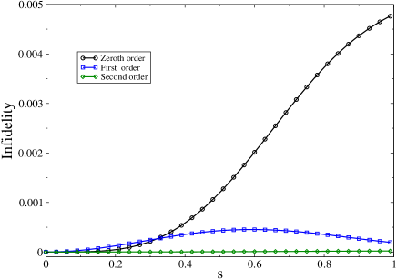
Figure 2: (Color online) Here we work with a constant gap ($\lambda=0$) and $\hbar=1.0$, $\theta_{0}=0.1$, $E_{0}=1.5$ and $v=w=0.5$, giving $\epsilon\approx 0.47$. Note that by including higher order terms in the perturbative series we get a better description of the evolved state. Here and in the following figures all quantities are dimensionless.

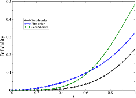
Figure 3: (Color online) Here $\lambda=0$, $\hbar=1.0$, $\theta_{0}=0.1$, $E_{0}=1.5$ and $v=w=1.5$ giving $\epsilon\approx 1.41$. Now the inclusion of higher order terms is detrimental since $\epsilon>1.$

Let us now work with a time-dependent gap, which can be achieved by setting $\lambda=1$ in Eq. (182). Within this choice of $\lambda$, we deal with two different scenarios. First we fix the minimum gap ($2E_{0}$) and successively solve Hamiltonian (178) for increasing $v$ (Fig. 4). Next we fix $v$ and solve (178) for different values of $E_{0}$ (Fig. 5).

In Fig. 4 we see that for all values of $v$ such that $\epsilon<1$ (upper panels), the more orders we include in the perturbative series the closer we get to the exact solution. And the lower $v$ the better the approximation. By increasing $v$ we arrive at a point where $\epsilon>1$ (lower panels) and we start to see the breaks down of DAPT, which becomes more manifest for greater values of $\epsilon$.

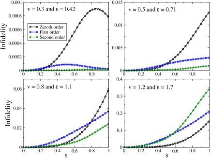
Figure 4: (Color online) Here $\lambda=\hbar=1.0$, $\theta_{0}=0.1$, $E_{0}=1.0$ and $v=w$. Note that as $\epsilon\rightarrow 1$ the perturbative series breaks down.

Finally, in Fig. 5 we clearly note that, for fixed $v$, the greater the minimum gap the better DAPT. By continually decreasing the gap we keep increasing $\epsilon$ until it gets larger than one. In such a case, as can be seen in the lower-right panel of Fig. 5, DAPT breaks down. For values of $\epsilon\approx 1$, but still lower than one, we need to include higher orders to get a good approximation; just keeping terms up to first order is not enough to outperform the zeroth order approximation during the whole time evolution (lower-left panel of Fig. 5).

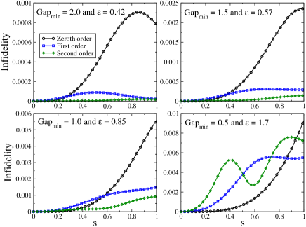
Figure 5: (Color online) Here $\lambda=\hbar=1.0$, $\theta_{0}=0.1$, and $v=w=0.3$. Note that as the gap ($2E_{0}$) increases the better DAPT describes the evolved state. For $\epsilon\gtrsim 1$ it no longer works. In the figure we see the values of $\epsilon$ calculated for the minimum gap.

IX Conclusions

We presented and expanded on the degenerate adiabatic perturbation theory (DAPT) first introduced in Ref. Rig10 , whose goal is to provide consistent perturbative corrections about the degenerate adiabatic approximation (DAA) for time-dependent systems. We provided all the missing mathematical steps leading to its development as well as new physical insights and a better understanding of concepts brought forth by DAPT. In particular, we emphasized the importance of three key ingredients without which the development of DAPT would be doomed to failure.

First, we showed the importance of a proper rescaling of the time $s=vt$ in the Schrödinger equation (SE) in terms of the adiabatic parameter $v=1/T$, which is related to the rate (“velocity”) at which the Hamiltonian $\mathbf{H}(t)$ is driven from its initial to its final configuration, and upon which the perturbative series is built. On the formal level, this rescaling allowed us to properly identify the correct order in the perturbative series.

This rate depends on intrinsic internal parameters of $\mathbf{H}(t)$ which ultimately reflects on how $\mathbf{H}(t)$ changes along the parameter space in order to reach a given final configuration. Indeed, it is a delicate balance between the rate at which $\mathbf{H}(t)$ changes and the duration $T$ of the whole time evolution (experiment) what dictates whether DAPT converges or not and, hence, furnishes meaningful perturbative corrections about DAA. Reversing the argument of the previous sentence, a failure of DAPT to converge may indicate that for a given $\mathbf{H}(t)$ and experimental running time $T$ the system’s evolution cannot be approximated by DAA. In such a case, for the system to be well approximated by DAA and the leading orders of DAPT, we should slow down the rate at which $\mathbf{H}(t)$ changes by decreasing $v$, which manifests itself in a longer experimental running time (greater $T$).

Second, in order to make any progress we had to propose the right ansatz with a compact and clear notation for ease of later mathematical manipulations; one that had at the same time the following two characteristics. On one hand it should correctly deal with the rescaled time $s$ and perturbative parameter $v$. As such, it should factor out terms of order $\mathcal{O}(v^{-1})$ and below, which are the problematic ones when $v\rightarrow 0$, i.e., when the system’s evolution should be well described by DAA. On the other hand, the ansatz should lead to computable higher order corrections in a straightforward and numerically robust manner. The ansatz we presented had these two properties allowing us to get recursive relations where the $p$-th order correction (the term multiplying $v^{p}$ in the perturbative series, $p\geq 1$) is obtained from knowledge of the order $p-1$.

Third, in contrast to many standard time-dependent perturbation theories, the right ansatz alone is not enough to guarantee the right perturbative corrections. It is of paramount importance to set the correct initial condition in the recursive relations. This is accomplished by imposing that at $t=0$ all higher order terms in the perturbative series expansion are zero with the exception of the zeroth order, which is tuned to satisfy the system’s initial condition. Also, for the rest of the system’s time evolution we must have that the zeroth order is DAA. This is achieved by building the zeroth order term in such a way that transitions among different eigenspaces are forbidden. With this choice the non-abelian Wilczek-Zee (WZ) geometric phase naturally appears as the solution to the zeroth order recursive relation.

In addition to the formal development of DAPT, which allowed us to correctly determine perturbative corrections about DAA, the ideas summarized in the previous paragraphs paved the ground to a rigorous formulation of the adiabatic theorem of quantum mechanics for non-degenerate and degenerate systems. With the aid of DAPT, we were able to formulate and prove necessary and sufficient conditions for the validity of the degenerate adiabatic theorem (DAT) Rig12 . A more extensive discussion of DAT and its physical meaning, in particular the notion of slowly changing Hamiltonians, as well as all technical details of the proofs outlined in Rig12 were presented in Sec. VI.

In the remaining sections of this paper we applied both DAPT and the conditions for the validity of DAT to a few examples. We derived in full detail the exact closed form solution Rig10 to a degenerate time-dependent problem Bis89 , which is a natural extension of the famous non-degenerate spin-1/2 system subjected to a rotating external magnetic field Rab54 . We then verified that DAPT gives the correct perturbative corrections to this model, matching exactly the expansion of the exact solution in terms of $v$. Furthermore, we applied the necessary and sufficient conditions for the validity of DAT to this model and showed that they give the correct conditions under which DAA is a good description for the system’s evolution. We then solved numerically several time-dependent Hamiltonians in order to compare their solutions with the perturbative series derived from DAPT. We showed that for small enough $v$ DAPT gives excellent results by just truncating the perturbative series at the second order. Finally, we should mention that the study of both the exactly solvable model and the numerical ones allowed us to have a better grasp of the meaning of $v$ and also understand the conditions under which DAPT provides meaningful results.

Appendix A The Wilczek-Zee Phase

We can write the most general state describing a degenerate system as (cf. Eq. (4)),

$$\mathbf{|\Psi}(t)\rangle=\sum_{n=0}\mathrm{e}^{-\mathrm{i}\omega_{n}(t)}b_{n}(t)\mathbf{U}^{n}(t)\mathbf{|n}(t)\rangle,$$ (200)

with the dynamical phase $\omega_{n}(t)$ given by Eq. (5) (for the moment we make no assumptions about the other quantities). To proceed, we need to work with the transposed quantities (cf. Sec. V). Thus,

$$\mathbf{|\Psi}(t)\rangle^{T}=\sum_{n=0}\mathrm{e}^{-\mathrm{i}\omega_{n}(t)}b_{n}(t)\mathbf{|n}(t)\rangle^{T}\mathbf{U}^{n}(t)^{T}.$$ (201)

Transposing SE, Eq. (10), inserting Eq. (201) into it, and left multiplying both sides by $\langle\mathbf{m}(t)|^{T}$, we get after exchanging $n\leftrightarrow m$ and transposing back,

$$\dot{b}_{n}(t)\mathbf{U}^{n}(t) + b_{n}(t)\dot{\mathbf{U}}^{n}(t)$$

$$+ \sum_{m=0}b_{m}(t)\mathrm{e}^{-\mathrm{i}\omega_{mn}(t)}\mathbf{U}^{m}(t)\mathbf{M}^{mn}(t)=0,$$

with $\omega_{mn}(t)=\omega_{m}(t)-\omega_{n}(t)$ and $\mathbf{M}^{mn}(t)$ given by Eq. (7). So far no approximation has been made and, in principle, the time evolution could be determined by solving the system of differential equations given in (LABEL:ap3).

The degenerate adiabatic approximation (DAA) consists in neglecting the coupling between different eigenspaces $\mathcal{H}_{n}$ but not those within a given eigenspace, i.e., we must have

$$\mathbf{M}^{nm}(t)\approx\delta_{nm}\mathbf{M}^{nn}(t)\hskip 14.22636pt\text{and}\hskip 14.22636ptb_{n}(t)\approx b_{n}(0).$$ (203)

Inserting Eq. (203) into (LABEL:ap3) gives,

$$\dot{\mathbf{U}}^{n}(t)-\mathbf{U}^{n}(t)\mathbf{A}^{nn}(t)=0,$$ (204)

where we defined $\mathbf{A}^{nm}(t)=-\mathbf{M}^{nm}(t)$. The previous differential equation is nothing but the Wilczek-Zee (WZ) phase, whose formal solution is written as Wil84

$$\mathbf{U}^{n}(t)=\mathbf{U}^{n}(0)\mathcal{T}\exp\left(\int_{0}^{t}\mathbf{A}^{nn}(t^{\prime})dt^{\prime}\right),$$ (205)

with $\mathcal{T}$ denoting time-ordering. We should note that in Ref. Wil84 the authors assume that the system is initialized in an eigenvector of $\mathbf{H}(t)$. Here we relax this assumption (Eq. (200)). It is by using conditions (203) that we derive the WZ phase and establish that the system evolves according to Eq. (4).

The previous approach, however, does not provide a rigorous way to get necessary and sufficient conditions guaranteeing that the system’s evolution can be approximated by Eq. (4). And the reason is simple: in general we do not have the solution to SE that leads to the explicit formula for $b_{n}(t)$. All we can do is to test whether the first piece of Eq. (203), the one that can be computed without knowing the solution to the SE, is a valid approximation. In other words, if for $n\neq m$ and all $t$

$$\mathbf{M}^{nm}(t)\ll 1,$$

then DAA is probably a good description of the system’s evolution. But we can get into trouble because this does not necessarily imply

$$\dot{b}_{n}(t)\ll 1.$$

Rigorous conditions and how much we are losing by neglecting higher order terms can be obtained, though, by using DAPT (cf. Secs. V and VI).

Appendix B Proof that DAPT implies APT

The non-degenerate ansatz of APT as given in Rig08 is

$$|\Psi(s)\rangle=\sum_{n,m=0}\sum_{p=0}^{\infty}v^{p}\mathrm{e}^{-\frac{\mathrm{i}}{v}\omega_{m}(s)}\mathrm{e}^{\mathrm{i}\gamma_{m}(s)}b_{nm}^{(p)}(s)|n(s)\rangle,$$ (206)

with $\gamma_{m}(s)$ the Berry phase, i.e., Eq. (6) when no degeneracy is present. In the present notation, this ansatz led to the following recursive relation Rig08

$$\frac{\mathrm{i}}{\hbar}\Delta_{nm}(s)b_{nm}^{(p+1)}(s) + \dot{b}^{(p)}_{nm}(s)-[\mathbf{M}^{mm}(s)]_{00}b_{nm}^{(p)}(s)$$ (207)

$$+ \sum_{k=0}b_{km}^{(p)}(s)[\mathbf{M}^{kn}(s)]_{00}=0,$$

with the following zeroth order term

$$b_{nm}^{(0)}(s)=b_{n}(0)\delta_{nm}.$$ (208)

To prove that APT is a particular case of DAPT we need to show that Eqs. (206)-(208) are equivalent to the ones derived from DAPT when we assume no-degeneracy.

First, comparing Eq. (206) with DAPT ansatz (15) we note that we must have

$$\mathbf{B}_{mn}^{(p)}(s)=\mathrm{e}^{\mathrm{i}\gamma_{m}(s)}b_{nm}^{(p)}(s)$$ (209)

for them to be equivalent. Inserting Eq. (209) into (207) and noting that $\dot{\gamma}_{m}(s)=\mathrm{i}[\mathbf{M}^{mm}(s)]_{00}$ leads to

$$\frac{\mathrm{i}}{\hbar}\Delta_{nm}(s)\mathbf{B}_{mn}^{(p+1)}(s)+\dot{\mathbf{B}}^{(p)}_{mn}(s)\\ +\sum_{k=0}\mathbf{B}_{mk}^{(p)}(s)\mathbf{M}^{kn}(s)=0,$$

which is exactly the recursive relation (25) of DAPT.

Finally, for $p=0$ if we insert (208) into (209) we get DAPT zeroth order noting that for non-degenerate systems $\mathbf{U}^{n}(s)=\mathrm{e}^{\mathrm{i}\gamma_{n}(s)}$.

Appendix C General solution to the recursive relation

Our goal here is to manipulate Eq. (25) to explicitly obtain $\mathbf{B}_{mn}^{(p+1)}(s)$ in terms of the lower order coefficients. For $n\neq m$, Eq. (25) straightforwardly implies

$$\mathbf{B}_{mn}^{(p+1)}(s) = \frac{\mathrm{i}\hbar}{\Delta_{nm}(s)}\left(\dot{\mathbf{B}}_{mn}^{(p)}(s)+\sum_{k=0}\mathbf{B}_{mk}^{(p)}(s)\mathbf{M}^{kn}(s)\right).$$

(210)

When $n=m$, Eq. (25) gives

$$\dot{\mathbf{B}}_{nn}^{(p+1)}(s) + \mathbf{B}_{nn}^{(p+1)}(s)\mathbf{M}^{nn}(s)$$ (211)

$$+ \mathop{\sum_{k=0}}_{k\neq n}\mathbf{B}_{nk}^{(p+1)}(s)\mathbf{M}^{kn}(s)=0.$$

Making the following change of variable

$$\mathbf{B}_{nn}^{(p+1)}(s)=\mathbf{\tilde{B}}_{nn}^{(p+1)}(s)\mathbf{U}^{n}(s)$$ (212)

leads to

$$\mathbf{\tilde{B}}_{nn}^{(p+1)}(s)\!\left(\!\dot{\mathbf{U}}^{n}(s)+\mathbf{U}^{n}(s)\mathbf{M}^{nn}(s)\!\right)+\mathbf{\dot{\tilde{B}}}_{nn}^{(p+1)}(s)\mathbf{U}^{n}(s)$$ (213)

$$+ \mathop{\sum_{k=0}}_{k\neq n}\mathbf{B}_{nk}^{(p+1)}(s)\mathbf{M}^{kn}(s)=0.$$

The term inside the parenthesis is zero since $\mathbf{U}^{n}(s)$ is the WZ-phase (cf. Eq. (204)). Then, using the unitarity of $\mathbf{U}^{n}(s)$, we can solve for $\mathbf{\tilde{B}}_{nn}^{(p+1)}(s)$,

$$\mathbf{\tilde{B}}_{nn}^{(p+1)}(s)=\mathbf{\tilde{B}}_{nn}^{(p+1)}(0)-\mathop{\sum_{m=0}}_{m\neq n}\int_{0}^{s}\mathbf{B}_{nm}^{(p+1)}(s^{\prime})\mathbf{M}^{mn}(s^{\prime})\left(\mathbf{U}^{n}(s^{\prime})\right)^{\dagger}\mathrm{d}s^{\prime},$$ (214)

where we have changed $k\rightarrow m$. Then, returning to the original variable

$$\mathbf{B}_{nn}^{(p+1)}(s)=-\mathop{\sum_{m=0}}_{m\neq n}\mathbf{B}_{mn}^{(p+1)}(0)\left(\mathbf{U}^{n}(0)\right)^{\dagger}\mathbf{U}^{n}(s)-\mathop{\sum_{m=0}}_{m\neq n}\int_{0}^{s}\mathrm{d}s^{\prime}\left(\mathbf{B}_{nm}^{(p+1)}(s^{\prime})\mathbf{M}^{mn}(s^{\prime})\left(\mathbf{U}^{n}(s^{\prime})\right)^{\dagger}\right)\mathbf{U}^{n}(s),$$ (215)

where we have written the initial condition (16) as

$$\mathbf{\tilde{B}}_{nn}^{(p+1)}(0)=-\mathop{\sum_{m=0}}_{m\neq n}\mathbf{\tilde{B}}_{mn}^{(p+1)}(0)\left(\mathbf{U}^{n}(0)\right)^{\dagger}.$$ (216)

Finally, using Eq. (210) we get

$$\mathbf{B}_{nn}^{(p+1)}(s) = -\mathrm{i}\hbar\mathop{\sum_{m=0}}_{m\neq n}\frac{\dot{\mathbf{B}}_{mn}^{(p)}(0)\left(\mathbf{U}^{n}(0)\right)^{\dagger}\mathbf{U}^{n}(s)}{\Delta_{nm}(0)}-\mathrm{i}\hbar\mathop{\sum_{m=0}}_{m\neq n}\sum_{k=0}\frac{\mathbf{B}_{mk}^{(p)}(0)\mathbf{M}^{kn}(0)\left(\mathbf{U}^{n}(0)\right)^{\dagger}\mathbf{U}^{n}(s)}{\Delta_{nm}(0)}$$ (217)

$$+\mathrm{i}\hbar\mathop{\sum_{m=0}}_{m\neq n}\int_{0}^{s}\left(\frac{\dot{\mathbf{B}}_{nm}^{(p)}(s^{\prime})\mathbf{M}^{mn}(s^{\prime})\left(\mathbf{U}^{n}(s^{\prime})\right)^{\dagger}}{\Delta_{nm}(s^{\prime})}\right)\mathrm{d}s^{\prime}\mathbf{U}^{n}(s)$$

$$+\mathrm{i}\hbar\mathop{\sum_{m=0}}_{m\neq n}\sum_{k=0}\int_{0}^{s}\left(\frac{\mathbf{B}_{nk}^{(p)}(s^{\prime})\mathbf{M}^{km}(s^{\prime})\mathbf{M}^{mn}(s^{\prime})\left(\mathbf{U}^{n}(s^{\prime})\right)^{\dagger}}{\Delta_{nm}(s^{\prime})}\right)\mathrm{d}s^{\prime}\mathbf{U}^{n}(s).$$

Equations (210) and (217), together with the zeroth order term (Eq. (16)), $\mathbf{B}_{mn}^{(0)}(s)=b_{n}(0)\mathbf{U}^{n}(s)\delta_{mn},$ are all that we need to get perturbative corrections about DAA to any order. However, in many applications of DAPT, it is easier to use the recursive relation (25) directly.

Appendix D $\theta\approx 0$ does not imply $|\Psi(t)\rangle\approx|\Psi^{(0)}(t)\rangle$

Expanding up to first order in $\theta$ DAA, Eq. (144), and the exact solution, Eq. (112), we get respectively

$$|\Psi^{(0)}(t)\rangle = \mathrm{e}^{\frac{\mathrm{i}bt}{2}}|0^{0}(t)\rangle+\mathrm{i}\theta\mathrm{e}^{-\frac{1}{2}\mathrm{i}(w-b)t}\sin\left(\frac{wt}{2}\right)|0^{1}(t)\rangle,$$

$$|\Psi(t)\rangle = |\Psi^{(0)}(t)\rangle+\frac{\mathrm{i}\theta w\mathrm{e}^{-\frac{1}{2}\mathrm{i}wt}\sin\left(\frac{1}{2}(w-b)t\right)}{w-b}|1^{1}(t)\rangle.$$

Comparing both expressions it is clear that if $w\geq b$ the probabilities to measure $|0^{1}(t)\rangle$ and $|1^{1}(t)\rangle$ are always of the same order in $\theta$ and, therefore, the system cannot be properly described by DAA. However, when $w\ll b$ it is clear that the probability to get $|1^{1}(t)\rangle$ vanishes and the one to obtain $|0^{1}(t)\rangle$ does not (there is no $b$ in its denominator). This shows, as expected, that for slowly rotating fields DAA is a good approximation to the system’s evolution.

References

• (1) C. Cohen-Tannoudji, B. Diu, and F. Laloë, Quantum Mechanics (John Wiley & Sons, New York, 1977), vol. 2.
• (2) A. Messiah, Quantum Mechanics (North-Holland, Amsterdam, 1962), vol. 2.
• (3) S. Jansen, M.-B. Ruskai, and R. Seiler, J. Math. Phys. 48, 102111 (2007).
• (4) G. Rigolin, G. Ortiz, and V. H. Ponce, Phys. Rev. A 78, 052508 (2008).
• (5) C. De Grandi, V. Gritsev, and A. Polkovnikov, Phys. Rev. B 81, 012303 (2010).
• (6) C. De Grandi and A. Polkovnikov, Lecture Notes in Physics 802, 75 (2010).
• (7) C. De Grandi, A. Polkovnikov, and A. W. Sandvik, Phys. Rev. B 84, 224303 (2011).
• (8) A. Polkovnikov, K. Sengupta, A. Silva, and M. Vengalattore, Rev. Mod. Phys. 83, 863 (2011).
• (9) G. Rigolin and G. Ortiz, Phys. Rev. Lett. 104, 170406 (2010).
• (10) D. M. Tong, Phys. Rev. Lett. 104, 120401 (2010).
• (11) G. Rigolin and G. Ortiz, Phys. Rev. A 85, 062111 (2012).
• (12) D. A. Ivanov, Phys. Rev. Lett. 86, 268 (2001).
• (13) E. Cobanera and G. Ortiz, Phys. Rev. A 89, 012328 (2014).
• (14) R. Unanyan, M. Fleischhauer, B. W. Shore, and K. Bergmann, Optics Commun. 155, 144 (1998).
• (15) R. G. Unanyan, B. W. Shore, and K. Bergmann, Phys. Rev. A 59, 2910 (1999).
• (16) Z. Kis, A. Karpati, B. W. Shore, and N. V. Vitanov, Phys. Rev. A 70, 053405 (2004).
• (17) I. Thanopulos, P. Král, and M. Shapiro, Phys. Rev. Lett. 92, 113003 (2004).
• (18) S. N. Biswas, Phys. Lett. B 228, 440 (1989).
• (19) M. V. Berry, Proc. R. Soc. Lond. A 392, 45 (1984).
• (20) F. Wilczek and A. Zee, Phys. Rev. Lett. 52, 2111 (1984).
• (21) F. Wilczek, Opening talk at Nobel Symposium 148, eprint: arXiv:1109.1523v1 [cond-mat.mes-hall].
• (22) D. J. Thouless, Phys. Rev. B 27, 6083 (1983).
• (23) D. Cheung, P. Høyer and N. Wiebe, J. Phys. A: Math. Theor. 44, 415302 (2011).
• (24) Due to the Kronecker delta appearing in Eq. (16) the rhs of (68) can also be written as $\sum_{m=0}|[\mathbf{B}_{mn}^{(0)}(s)]_{0g_{n}}|$. This is how it is presented in Rig12 .
• (25) I. I. Rabi, N. F. Ramsey, and J. Schwinger, Rev. Mod. Phys. 26, 167 (1954).
• (26) A. Bohm, Quantum Mechanics: Foundations and Applications (Springer-Verlag, New York, 1993), p. 587.
• (27) V. I. Yukalov, Phys. Rev. A 79, 052117 (2009).