Random walks with preferential relocations to places visited in the past and their application to biology

Abstract

Strongly non-Markovian random walks offer a promising modeling framework for understanding animal and human mobility, yet, few analytical results are available for these processes. Here we solve exactly a model with long range memory where a random walker intermittently revisits previously visited sites according to a reinforced rule. The emergence of frequently visited locations generates very slow diffusion, logarithmic in time, whereas the walker probability density tends to a Gaussian. This scaling form does not emerge from the Central Limit Theorem but from an unusual balance between random and long-range memory steps. In single trajectories, occupation patterns are heterogeneous and have a scale-free structure. The model exhibits good agreement with data of free-ranging capuchin monkeys.

The individual displacements of living organisms exhibit rich statistical features over multiple temporal and spatial scales. Due to their seemingly erratic nature, animal movements are often interpreted as random search processes and modeled as random walks turchin ; colding ; randomsearch . In recent years, the increasing availability of data on animal interm4 ; nathan ; sims ; weimer as well as human geisel ; gonzalez ; song1 ; song mobility have motivated numerous models inspired from the simple random walk (RW). Let us mention, in particular, multiple scales RWs, such as Lévy walks levy1 ; levy2 or intermittent RWs interm4 ; interm1 ; interm2 ; interm3 , which are walks with short local movements mixed with less frequent but longer commuting displacements.

Markovian RWs are the basic paradigm for modeling animal and human mobility and they provide useful insights at short temporal scales. However, empirical studies conducted over long periods of times reveal pronounced non-Markovian effects song ; chinos ; interface . As for humans, mounting evidence shows that many animals have sophisticated cognitive abilities and use memory to move to familiar places that are not in their immediate perception range fagan ; janson . The use of long-term memory should strongly impact movement and it is probably at the origin of many observations which are incompatible with RWs predictions, such as, very slow diffusion, heterogeneous space use, the tendency to revisit often particular places at the expense of others, or the emergence of routines gautestad2005 ; gautestad2006 ; song1 ; song ; chinos ; interface . Non-Markovian random walks where movement steps depend on the whole path of the walker elephant1 ; elephant2 ; italian offer a promising modeling framework in this context. But the relative lack of available analytical results in this area limits the understanding of the effects of memory on mobility patterns.

Self-attracting or reinforced RWs are an important class of non-Markovian dynamics annals . In these processes, typically, a walker on a lattice moves to a nearest-neighbor site with a probability that depends on the number of times this site has been visited in the past davis ; siam ; epl . These walks must be in principle described by a hierarchy of multiple-time distribution functions, or can be studied within field theory approaches nuovo . In a slightly different context, some exact results have been obtained for the mean square displacement (MSD) in globally reinforced models, such as the so-called elephant walk elephant1 ; elephant2 , where the walker tends to move in the same direction than the sum of all its previous movement steps.

Figure 1: (Color online) A model walker combining random steps to nearest neighbor sites and relocations, at a rate $q$, to sites visited in the past (marked in light color).

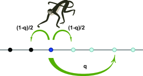
In this Letter we solve a minimal, lattice version of a reinforced model proposed some time ago in the ecological literature gautestad2005 ; gautestad2006 , where a walker can either move randomly (explore locally) or stochastically relocate to places visited in the past (via long distance steps). A constant parameter describes the relative rate of these two movement modes (Fig. 1). This RW model with long range memory is, to our knowledge, one of the very few where not only the MSD is derived exactly, but also the asymptotic form of the full probability density. We then compare the model with field data and infer the strength of memory use in real animals.

We consider a walker with position ${\mathbf{X}}_{t}$ at time $t$ on a regular $d$-dimensional lattice with unit spacing, and initially located at ${\mathbf{X}}_{0}={\mathbf{0}}$. Consider $q$ a constant parameter, $0<q<1$. At each discrete time step, $t\rightarrow t+1$, the walker decides with probability $1-q$ to visit a randomly chosen nearest neighbor site, as in the standard RW. With the complementary probability $q$, the walker relocates directly to a site visited in the past (Fig. 1). In this case, the probability to choose a given lattice site, among all the visited sites, is proportional to the number of visits this site has already received in the interval $[0,t]$. It is thus more likely to revisit a site which has been visited many times than a site visited only once. This linear preferential revisit rule is equivalent to choosing a random integer $t^{\prime}$ uniformly in the interval $[0,t]$ and to return to the site occupied at $t^{\prime}$. This model bears some similarities with that of ref. evansmaj , where a RW is stochastically “reset” to the origin ($t^{\prime}=0$) at a constant rate. Here, the RW can be reset to any previous time, or visited site, thus making the process highly non-Markovian.

We summarize our main results in $1d$ for this model, where memory profoundly modifies the normal diffusion process and generates complex patterns of space occupation. (The results naturally extend to higher dimensions.) Let $P(n,t)$ be the probability that $X_{t}=n$. The MSD, defined as the ensemble average $\langle X_{t}^{2}\rangle=M_{2}(t)\equiv\sum_{n=-\infty}^{\infty}n^{2}P(n,t)$, is calculated exactly for all $t$. Asymptotically, it grows very slowly with time:

$$M_{2}(t)\simeq\frac{1-q}{q}\left[\ln(qt)+\gamma\right],\quad t\gg 1,$$ (1)

with $\gamma=0.5772...$ the Euler constant. In addition, the distribution $P(n,t)$ tends to a Gaussian, as in normal diffusion, but with a variance given by the anomalous logarithmic law (1) instead of the usual normal law $\propto t$:

$$P(n,t)\rightarrow G(n,t)\equiv\frac{1}{\sqrt{2\pi M_{2}(t)}}\ e^{-\frac{n^{2}}{2M_{2}(t)}},$$ (2)

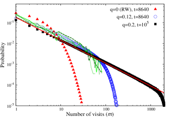
Notably, the mechanism that makes the process eventually Gaussian is driven by memory and thus markedly differs from the Central Limit Theorem. In particular, the convergence toward this scaling form is logarithmically slow in time, thus it is difficult to observe in practice in discrete time simulations. We also study the probability $P^{(v)}_{t}(m)$ that a site, randomly chosen among the sites visited by a single walker in $[0,t]$, has received exactly $m$ visits. Numerical results in $2d$ suggest a power-law behavior:

$$P^{(v)}_{t}(m)\propto m^{-\alpha},\quad{\rm with}\quad\alpha\simeq 1.1,$$ (3)

which indicates that the walker occupies space in a very heterogeneous way. The model in $2d$ agrees quantitatively with trajectory data of capuchin monkeys (Cebus capucinus) in the wild.

We next present a derivation of the results. In contrast with most path-dependent processes, here, a closed and exact master equation can be written for $P(n,t)$, see the Supplemental Material. In $1d$, it reads:

$$P(n,t+1) = \frac{1-q}{2}P(n-1,t)+\frac{1-q}{2}P(n+1,t)$$ (4)

$$+ \frac{q}{t+1}\sum_{t^{\prime}=0}^{t}P(n,t^{\prime}).\$$

The last term in Eq.(4) indicates that site $n$ can be visited (from any other site) following the memory rule provided that the walker was at $n$ at an earlier time $t^{\prime}$.

We define the even moments of the distribution as $M_{2p}(t)=\sum_{n=-\infty}^{\infty}n^{2p}P(n,t)$ with $p$ a positive integer ($M_{2p+1}(t)=0$ by symmetry).

Mean square displacement.$-$Taking the second moment of Eq.(4), we obtain an evolution equation for the MSD:

$$M_{2}(t+1)=1-q+(1-q)M_{2}(t)+\frac{q}{t+1}\sum_{t^{\prime}=0}^{t}M_{2}(t^{\prime}),$$ (5)

where we have used the normalization condition $M_{0}(t)=1$. The above equation can be solved by introducing the Z-transform of $M_{2}(t)$, defined as $\widetilde{M}_{2}(\lambda)=\sum_{t=0}^{\infty}\lambda^{t}M_{2}(t)$. Transforming Eq.(5) and using the identity $\lambda^{t}/(t+1)=\lambda^{-1}\int_{0}^{\lambda}u^{t}du$, one obtains:

$$\frac{\widetilde{M}_{2}(\lambda)}{\lambda}=\frac{1-q}{1-\lambda}+(1-q)\widetilde{M}_{2}(\lambda)+\frac{q}{\lambda}\int_{0}^{\lambda}du\frac{\widetilde{M}_{2}(u)}{1-u}.$$ (6)

This equation becomes a first order ordinary differential equation after taking a derivative with respect to $\lambda$. As $M_{2}(t=0)=0$, the condition to be fulfilled by the solution of Eq. (6) is $\widetilde{M}_{2}(\lambda=0)=0$. One finds:

$$\widetilde{M}_{2}(\lambda)=-\left(\frac{1-q}{q}\right)\frac{\ln(1-\lambda)-\ln[1-(1-q)\lambda]}{1-\lambda}.$$ (7)

The function $f(t)$ such that $\sum_{t=0}^{\infty}\lambda^{t}f(t)=\ln[1-(1-q)\lambda]/(1-\lambda)$, is $f(t)=-\sum_{k=1}^{t}(1-q)^{k}/k$. Therefore, Eq.(7) can be inverted, giving the exact solution:

$$M_{2}(t)=\frac{1-q}{q}\sum_{k=1}^{t}\frac{1-(1-q)^{k}}{k}.$$ (8)

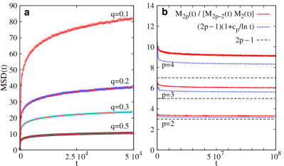
At large $t$, $\sum_{k=1}^{t}1/k\simeq\ln t+\gamma$ and $\sum_{k=1}^{t}(1-q)^{k}/k\simeq-\ln q$, yielding the asymptotic behavior (1) up to order $(\ln t)^{0}$. This result holds in any spatial dimensions. Figure 2a displays Eq.(1) for several values of $q$, in very good agreement with numerical simulations. Despite of the random steps, at any finite $q$, memory induces frequent returns to the same sites and very slow diffusion.

Figure 2: (Color online) a) MSD as a function of time for different memory strengths $q$. Symbols represent simulation results and the solid lines Eq. (1). b) Time evolution of the moment ratio for $p=2,3$ and $4$ from simulations with $q=0.1$ (solid red line) and the first order calculation Eq. (13) (dotted line). The curves tend to $2p-1$ at very large $t$.

Higher moments.$-$The asymptotic form of the propagator $P(n,t)$ can be extracted in principle from the knowledge of all its moments at large $t$. We first assume that a scaling relation is satisfied for $t$ large enough:

$$M_{2p}(t)\simeq a_{p}[M_{2}(t)]^{p},$$ (9)

for any integer $p$, with $a_{p}$ a constant. A well-known property of the Gaussian distribution with zero mean and arbitrary variance is that of having $a_{0}=1$ and

$$a_{p}=(2p-1)a_{p-1},\ \ p\geq 1.$$ (10)

We take the $2p$-th moment of Eq.(4):

$$M_{2p}(t+1) - M_{2p}(t)=1-q+(1-q)\sum_{k=1}^{p-1}C_{2p}^{2k}M_{2k}(t)$$ (11)

$$+ \frac{q}{t+1}\sum_{t^{\prime}=0}^{t}[M_{2p}(t^{\prime})-M_{2p}(t)].$$

Since $M_{2}(t)$ diverges at large $t$, from (9) the leading term in the first sum of (11) is that with $k=p-1$, like in the simple RW. But unlike in the RW, the left-hand-side $M_{2p}(t+1)-M_{2p}(t)\rightarrow 0$ and can be neglected, since it is $\simeq dM_{2p}/dt\propto(\ln t)^{p-1}/t$. Thus, using Eqs. (9) and (1), Eq. (11) gives the following relation for the $a_{p}$’s:

$$a_{p}=p(2p-1)a_{p-1}\lim_{t\rightarrow\infty}\frac{(t+1)(\ln t)^{p-1}}{\sum_{t^{\prime}=cst}^{t^{\prime}=t}[(\ln t)^{p}-(\ln t^{\prime})^{p}]}.$$ (12)

The limit in (12) turns out to be $1/p$ abram . Therefore relation (10) is obtained, implying the Gaussian form (2). This analysis illustrates that, here, Gaussianity is not the result of random increments producing fluctuations that scale as $\sqrt{t}$, but rather emerges in a process with very small fluctuations (of order $\sqrt{\ln t}$) from a balance between purely random steps and recurrent memory steps.

To examine how $a_{p}/a_{p-1}$ converges towards $2p-1$, we relax the condition that $a_{p}$ is constant. Assuming that $da_{p}(t)/dt$ does not decay slower than an inverse power law of time, one can still neglect the left-hand-side of (11). Keeping the terms of order $(\ln t)^{p-1}$ and $(\ln t)^{p-2}$, the leading time-dependent correction is obtained:

$$\frac{a_{p}}{a_{p-1}}(t)=(2p-1)\left(1+\frac{c_{p}}{\ln t}\right)+O((\ln t)^{-2})$$ (13)

with $c_{p}=(p-1)[1+q/6(1-q)]$. We see from (13) that the distribution $P(n,t)$ converges extremely slowly toward the Gaussian form (typically after $t\sim 10^{100}$), due to corrections of order $1/\ln t$ in the moment relations. In standard sums of random variables, these corrections are $O(1/\sqrt{t})$. Figure 2b displays the quotient $Q_{p}(t)\equiv M_{2p}(t)/[M_{2p-2}(t)M_{2}(t)]$ obtained from numerical simulations as a function of time, for $p=2,3$ and $4$. If a scaling relation (9) strictly holds, $Q_{p}(t)=a_{p}/a_{p-1}$. At $t=10^{8}$, $Q_{p}(t)$ still differs significantly from $2p-1$. Fig. 2b also displays $\frac{a_{p}}{a_{p-1}}(t)$ as given by formula (13). What seems to be a plateau at a constant value $>2p-1$ is actually a very slowly decaying function. The differences between the simulation and the analytical results are due to terms $O((\ln t)^{-2})$ or higher, which are not that small.

Figure 3: (Color online) a) TASD of radio-collared capuchin monkeys (dotted lines) and of the model walker (symbols) in $2d$ with the time step set to $\Delta t=30$ min and the cell size to $50$m$\times 50$m. The solid black line is the MSD of the model with $q=0.12$. b) Number of distinct cells visited by the monkeys and the simulated model walker with the parameters of a).

Monkey mobility data.$-$The very slow growth of the MSD with $t$ in our model agrees qualitatively with the fact that most animals have limited diffusion or home ranges moorcroftlewis ; gautestad2005 ; borger ; vanmoorter ; interface . We further compare the model predictions with trajectories of real animals in the wild. The displacements of four radio-collared capuchin monkeys were recorded during a period of six months in Barro Colorado Island, Panama. Discretized $2d$ positions, with resolution $\Delta\ell=50$ m were recorded every 10 min (see megpnas ; interface for details). Since no ensemble averages can be performed, we calculated for each individual monkey the time-averaged square displacement (TASD), noted as $\overline{\delta^{2}}(t)$, along each trajectory interface . We also calculated this quantity for simulated $2d$ walks in the model:

$$\overline{\delta^{2}}(t)\equiv\frac{1}{N-t}\sum_{i=1}^{N-t}|{\mathbf{X}}_{i+t}-{\mathbf{X}}_{i}|^{2},$$ (14)

with $N$ the total number of positions, and then obtained the numerical $\langle\overline{\delta^{2}}(t)\rangle$ by averaging over many walks. This quantity is a priori different from the MSD.

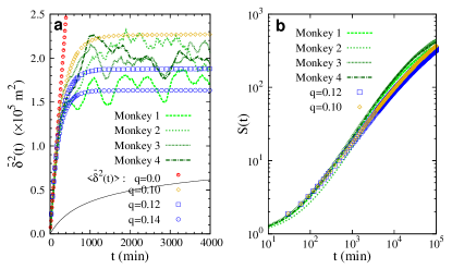
In Fig. 3a, the animals have a Brownian regime with $\overline{\delta^{2}}(t)\simeq 4Dt$ at short times, with a diffusion coefficient $D\simeq 300$ m${}^{2}/$min for all four monkeys, followed by a saturation at a roughly constant value. Setting the lattice spacing $\Delta\ell=50$ m in the model, too, the model time step is adjusted to $\Delta t=30$ min so that $\langle\overline{\delta^{2}}(t)\rangle$ matches the monkeys TASD at short times (hence, the 6 months of foraging data correspond to $N=8640$). These parameters being fixed, the value $q\simeq 0.12\pm 0.02$ best describes the monkeys TASD over the entire time range (Fig. 3a). The resulting relocation rate $r\equiv q/\Delta t\simeq 0.004$ min^-1 is low, suggesting that memory use by capuchin monkeys is intermittent. But even this small $r$ strongly affects diffusion after a few hours.

We note at this point that the model is non-ergodic, in the sense that $\langle\overline{\delta^{2}}(t)\rangle\neq M_{2}(t)$ godec . Here $\langle\overline{\delta^{2}}(t)\rangle$ quickly reaches a plateau, whereas $M_{2}(t)$ is smaller and slowly grows with $t$, as shown in Fig. 3a with $q=0.12$. Another criteria of non-ergodicity involves an ergodicity breaking parameter, which measures the fluctuations among time averages obtained from different trajectories: $EB\equiv\langle[\overline{\delta^{2}}(t)]^{2}\rangle/\langle\overline{\delta^{2}}(t)\rangle^{2}-1$ he ; barkai . According to this criteria, a process is non-ergodic if $\lim_{N\rightarrow\infty}EB\neq 0$. Setting $q=0.12$ and $N=8640$ gives $EB=0.055$ for the model. We actually find that $EB\rightarrow 0$ as $N\rightarrow\infty$ (not shown). Hence, the model is ergodic in this second sense: different long trajectories have the same $\overline{\delta^{2}}(t)$ at short times (or $\overline{\delta^{2}}(t)\simeq\langle\overline{\delta^{2}}(t)\rangle$). Interestingly, this similitude is also observed in the four monkeys (see Fig. 3a).

Figure 4: (Color online) Probability that a visited site chosen at random has been visited $m$ times in $t$ walker steps. Open circles: model simulations with $q$ fitted in Fig. 3a and $t$ corresponding to 6 months. The monkey data is shown in dashed green lines. The solid (red) line has slope $-1.10$.

Figure 3b shows the number $S(t)$ of distinct sites visited by the model walker in $2d$ with the parameters fitted above, confirming the good agreement with empirical data. Further insight into the recurrent properties of these walks is given by the distribution function of the number $m$ of visits per site, $P^{(v)}_{t}(m)$. Scale-free distributions often are an outcome of preferential rules, such as in Yule processes yule ; simon or network growth models with preferential attachment barabasi ; leyvraz . In a model trajectory, many sites are visited only once whereas fewer sites are visited very often and thus likely to be visited again, giving rise to the formation of “hot-spots” of activity. We speculate that $P^{(v)}_{t}(m)$ in $2d$ is scale-free when $q\neq 0$. The exponent $\alpha$ introduced in Eq.(3) seems to be independent of $q$, as shown in Figure 4. The scaling regime is more extended for $q$ and $t$ large. Monkeys visitation patterns closely follow the theoretical law. Unlike in Yule processes or the reinforced walk with preferential visits of ref. song , spatial correlations are strong here (the sites near a hot-spot are likely to be visited often, too), making the analytical calculation of $P^{(v)}_{t}(m)$ quite challenging.

Discussion.$-$Motivated by the modeling of animal mobility, we have studied a minimal, solvable random walk model with infinite memory where the sites visited in the past are preferentially revisited. Memory induces very slow diffusion and slowly drives the process towards Gaussianity. This latter form contrasts with the scaling functions of Markovian RW models exhibiting logarithmic diffusion (e.g., the Sinai model sinai1 ; sinai2 ; sinai3 ) or stopped diffusion (e.g., the RW stochastically reset to the origin evansmaj ), which have exponential tails. Likewise, the scaling function of the elephant walk model elephant1 in the anomalous regime is not Gaussian, although its precise form is not known gandhiPRE . Our results point out a new mechanism for the emergence of Gaussian distributions, which could be generic in stochastic processes where a recurrent memory does not prevent fluctuations from diverging with time, but make them grow slower than a power-law. As a consequence, the process is asymptotically described by an effective Fokker-Planck equation with a time dependent diffusion coefficient, $D=\frac{1-q}{2qt}$, see Eqs. (1)-(2). Such an effective description is useful for studying first-passage properties effecFP . The aging properties of the model also deserve further study.

The primate mobility data presented here provide additional evidence that memory is a key factor for home range self-organization gautestad2005 ; gautestad2006 ; borger ; vanmoorter ; boyerwalsh ; oikos2013 . Our model suggests that the use of memory is likely to be intermittent in animals, and that even a very small rate $r$ can induce very slow diffusion and heterogeneous patterns of space occupation.

We thank M.C. Crofoot, L. Lacasa, H. Larralde, F. Leyvraz, G. Oshanin, I. Pérez-Castillo, A. Robledo, S. Thurner and P.D. Walsh for many fruitful discussions and D. Aguilar for technical support. This work was supported by the Grant IN103911 of the Universidad Nacional Autónoma de México.

References

- (1) P. Turchin, Quantitative analysis of movement. (Sunderland, MA. Sinauer Associates Inc, 1998).
- (2) E. A. Codling, M. J. Plank, and S. Benhamou, J. R. Soc. Interface 5, 813 (2008).
- (3) G. M. Viswanathan, M. G. E. da Luz, E. P. Raposo, and H. E. Stanley, The Physics of foraging (Cambridge, Cambridge, 2011).
- (4) J. M. Morales, D. T. Haydon, J. Frair, K. E. Holsinger, and J. M. Fryxell, Ecology 85, 2436 (2004).
- (5) R. Nathan et al., Proc. Natl. Acad. Sci. USA 105, 19052 (2008).
- (6) D. W. Sims et al., Nature 451, 1098 (2008).
- (7) N. E. Humphries, H. Weimerskirch, N. Queiroz, E. J. Southall, and D. W. Sims, Proc. Natl. Acad. Sci. USA 109, 7169 (2012).
- (8) D. Brockmann, L. Hufnagel, and T. Geisel, Nature 439, 462 (2006).
- (9) M. C. González, C. A. Hidalgo, and A.-L. Barabási, Nature 453, 779 (2008).
- (10) C. Song, Z. Qu, N. Blumm, and A.-L. Barabási, Science 327, 1018 (2010);
- (11) C. Song, T. Koren, P. Wang, and A.-L. Barabási, Nature Phys. 6, 818 (2010).
- (12) G. M. Viswanathan, E. P. Raposo, and M. G. E. da Luz, Phys. Life Rev. 5, 133 (2008).
- (13) F. Bartumeus, M. G. E. da Luz, G. M. Viswanathan, and J. Catalan, Ecology 86, 3078 (2005).
- (14) O. Bénichou, M. Coppey, M. Moreau, P.-H. Suet, and R. Voituriez, Phys. Rev. Lett. 94, 198101 (2005).
- (15) O. Bénichou, C. Loverdo, M. Moreau, and R. Voituriez, Rev. Mod. Phys. 83, 81 (2011).
- (16) F. Bartumeus, Oikos 118, 488 (2009).
- (17) X.-W. Wang, X.-P. Han, and B.-H. Wang PLoS ONE 9, e84954 (2014).
- (18) D. Boyer, M. C. Crofoot, and P. D. Walsh, J. R. Soc. Interface 9, 842-847 (2012).
- (19) C. H. Janson and R. Byrne, Anim. Cogn. 10, 357 (2007).
- (20) W. F. Fagan et al., Ecol. Lett. 16, 1316 (2013).
- (21) A. O. Gautestad and I. Mysterud, Am. Nat. 165, 44 (2005).
- (22) A. O. Gautestad and I. Mysterud, Ecol. Complex. 3, 44 (2006).
- (23) G. M. Schtz and S. Trimper, Phys. Rev. E 70, 045101(R) (2004).
- (24) J. C. Cressoni, M. A. A. da Silva, and G. M. Viswanathan, Phys. Rev. Lett. 98, 070603 (2007).
- (25) M. Serva, Phys. Rev. E 88, 052141 (2013).
- (26) E. Bolthausen and U. Schmock, Ann. Probab. 25, 531 (1997).
- (27) B. Davis, Probab. Theor. Related Fields 84, 203 (1990).
- (28) H. G. Othmer and A. Stevens, SIAM J. Appl. Math. 57, 1044 (1997).
- (29) J. Choi, J. I. Sohn, K. I. Goh, and I. M. Kim, EPL 99, 50001 (2012).
- (30) L. Peliti, J. Phys 46, 1469 (1985); L. Peliti and L. Pietronero, Riv. Nuovo Cimento 10, 1 (1987).
- (31) M. R. Evans and S. N. Majumdar, Phys. Rev. Lett. 106, 160601 (2011).
- (32) M. Abramowitz and I. A. Stegun, Handbook of mathematical functions (Dover, New York, 1970).
- (33) P. R. Moorcroft and M. A. Lewis, Mechanistic home range analysis (Princeton University Press, Princeton, 2006).
- (34) L. Brger, B. D. Dalziel, and J. M. Fryxell, Ecol. Lett. 11, 637 (2008).
- (35) B. van Moorter et al., Oikos 118, 641 (2009).
- (36) M. C. Crofoot, I. C. Gilby, M. C. Wikelski, and R. W. Kays, Proc. Natl. Acad. Sci. USA 105, 577 (2008).
- (37) A. Godec and R. Metzler, Phys. Rev. Lett. 110, 020603 (2013).
- (38) Y. He, S. Burov, R. Metzler, and E. Barkai, Phys. Rev. Lett. 101, 058101 (2008).
- (39) A. Rebenshtok and E. Barkai, Phys. Rev. Lett. 99, 210601 (2007).
- (40) G. U. Yule, Phil. Trans. R. Soc. (London) B 213, 21 (1925).
- (41) H. A. Simon, Biometrika 42, 425 (1955).
- (42) A.-L. Barabási and R. Albert, Science 286, 509 (1999).
- (43) P. L. Krapivsky, S. Redner, and F. Leyvraz, Phys. Rev. Lett. 85, 4629 (2000).
- (44) H. Kesten, Physica A 138, 299 (1986).
- (45) A. O. Golosov, Russ. Math. Surv. 41, 199 (1986).
- (46) P. Le Doussal, C. Monthus, and D. S. Fisher, Phys. Rev. E 59, 4795 (1999).
- (47) M. A. A. da Silva, J. C. Cressoni, G. M. Schtz, G. M. Viswanathan, and S. Trimper, Phys. Rev. E 88, 022115 (2013).
- (48) S. C. Lim and S. V. Muniandy, Phys. Rev. E 66, 021114 (2002).
- (49) D. Boyer and P. D. Walsh, Phil. Trans. R. Soc. A 368, 5645 (2010).
- (50) J. Nabe-Nielsen, J. Tougaard, J. Teilmann, K. Lucke, and M. C. Forchhammer, Oikos 122, 1307 (2013).