Non-Gaussianities of primordial perturbations and tensor sound speed

Abstract

We investigate the relation between the non-Gaussianities of the primordial perturbations and the sound speed of the tensor perturbations, that is, the propagation speed of the gravitational waves. We find that the sound speed of the tensor perturbations is directly related not to the auto-bispectrum of the tensor perturbations but to the cross-bispectrum of the primordial perturbations, especially, the scalar-tensor-tensor bispectrum. This result is in sharp contrast with the case of the scalar (curvature) perturbations, where their reduced sound speed enhances their auto-bispectrum. Our findings indicate that the scalar-tensor-tensor bispectrum can be a powerful tool to probe the sound speed of the tensor perturbations.

.1 Introduction

Inflation is now widely accepted as a paradigm of early Universe to explain the origin of the primordial perturbations as well as to solve the horizon and the flatness problems of the standard big-bang cosmology inflation . The current observational data such as the cosmic microwave background (CMB) anisotropies support almost scale-invariant, adiabatic, and Gaussian primordial curvature fluctuations as predicted by inflation. While the paradigm itself is well established and widely accepted, its detailed dynamics, e.g. the identification of an inflaton, its kinetic and potential structure, and its gravitational coupling, are still unknown.

The non-Gaussianities of primordial curvature perturbations are powerful tools to give such informations. It is well-known that the equilateral type of bispectrum of primordial curvature perturbations is enhanced by the inverse of their sound speed squared Seery:2005wm ; Chen:2006nt . The null observation of the equilateral type by the Planck satellite, characterized as $f^{\rm equil}_{\rm NL}=42\pm 75$ (68% CL) Ade:2013ydc , yields stringent constraints on the sound speed of the curvature perturbations as $c_{s}\geq 0.02$ (95% CL) Ade:2013ydc . The local type of bispectrum of primordial curvature perturbations also gives useful informations. Maldacena’s consistency relation Maldacena:2002vr ; Creminelli:2004yq says that the parameter $f_{\rm NL}^{\rm local}$ characterizing the local type of bispectrum is as much as ${\cal O}(0.01)$ for a single field inflation model. Though the current constraint on this parameter by the Planck satellite is already tight as $f_{\rm NL}^{\rm local}=2.7\pm 5.8$ (68% CL) Ade:2013ydc , the detection of non-Gaussianities with $f_{\rm NL}^{\rm local}\sim{\cal O}(1)$ by future observations would rule out a single field inflation model.

Inflation generates not only primordial curvature perturbations but also primordial tensor perturbations Starobinsky:1979ty . Very recently, it was reported that primordial tensor perturbations have been found and the tensor-to-scalar ratio $r$ is given by $r=0.20^{+0.07}_{-0.05}$ (68% CL) Ade:2014xna , though it is constrained as $r<0.11$(95% CL) in the Planck results Ade:2013uln . Their amplitude directly determines the energy scale of inflation, so it is estimated as $V^{1/4}\simeq 2.2\times 10^{16}$ GeV given $r\simeq 0.2$ Ade:2014xna and $P_{\zeta}\simeq 2.2\times 10^{-9}$ Ade:2013uln . If we go beyond the powerspectrum, it is known that the bispectra of primordial tensor perturbations enable us to probe the gravitational coupling of the inflaton field Gao:2011vs . Such a non-trivial gravitational coupling easily modifies the sound speed of primordial tensor perturbations, $c_{\gamma}$, and it can significantly deviate from unity Kobayashi:2011nu . Then, one may wonder if the small sound velocity of primordial tensor perturbations can enhance their non-Gaussianities as in the case of the curvature perturbations. In this Letter, we are going to address this issue.

The relation between the sound speed and the non-Gaussianities of primordial curvature perturbations can be clearly understood by use of the effective field theory (EFT) approach to inflation Cheung:2007st . Inflation can be characterized by the breakdown of time-diffeomorphism invariance due to the time-dependent cosmological background and the general action for inflation can be constructed based on this symmetry breaking structure. The primordial curvature perturbation can be identified with the Goldstone mode $\pi$ associated with the breaking of time-diffeomorphism invariance. The primordial curvature perturbation can be identified with the Goldstone mode $\pi$ associated with the breaking of time-diffeomorphism invariance. The symmetry arguments require that modification of the sound speed $c_{s}$ induces non-negligible cubic interactions of the Goldstone mode $\pi$, and hence the sound speed and the bispectrum of the curvature perturbations are directly related.

In this Letter, we investigate the relation between the sound speed of tensor perturbations and the bispectrum of primordial perturbations, based on the EFT approach. We first identify what kind of operators can modify the tensor sound speed. Then, we clarify which type of bispectrum arises associated with the modification and can be used as a probe for the tensor sound speed.

.2 The EFT approach

We start from a brief review of the EFT approach Cheung:2007st and clarify our setup. In the unitary gauge, where the inflaton field does not fluctuate, dynamical degrees of freedom in single-clock inflation are the metric field $g_{\mu\nu}$ only and the action should respect the (time-dependent) spatial diffeomorphism invariance. The action at the lowest order in perturbations can be uniquely determined by the background equations of motion and the residual spatial diffeomorphism invariance as

$$S_{0} =M_{\rm Pl}^{2}\int d^{4}x\sqrt{-g}\left[\frac{1}{2}R+\dot{H}g^{00}-(3H^{2}+\dot{H})\right]\,,$$ (1)

where $H(t)=\dot{a}/a$ is the background Hubble parameter with $a(t)$ being the the background scale factor

$$ds^{2}=-dt^{2}+a(t)^{2}d\vec{x}^{2}\,.$$ (2)

This simplest action describes tree-level dynamics of the single-field inflation with a canonical kinetic term in the Einstein gravity. Modifications of inflation models and quantum corrections can be described by including higher order perturbation terms. Ingredients for higher order perturbations are $\delta g^{00}$, $\delta K_{\mu\nu}$, $\delta R_{\mu\nu\rho\sigma}$, and their derivatives:

$$\delta g^{00}=g^{00}+1\,,\quad\delta K_{\mu\nu}=K_{\mu\nu}-Hh_{\mu\nu}\,,$$

$$\delta R_{\mu\nu\rho\sigma}=R_{\mu\nu\rho\sigma}-H^{2}(h_{\mu\rho}h_{\nu\sigma}-h_{\mu\sigma}h_{\nu\rho})$$

$$\qquad\qquad\,\,+(H^{2}+\dot{H})(h_{\mu\rho}n_{\nu}n_{\sigma}+\text{$3$ terms})\,,$$ (3)

which are covariant under the spatial diffeomorphism and vanish on the FRW background. Here $n_{\mu}=-\frac{\delta^{0}_{\mu}}{\sqrt{-g^{00}}}$ is the unit vector perpendicular to constant-$t$ surfaces, $h_{\mu\nu}=g_{\mu\nu}+n_{\mu}n_{\nu}$ is the induced spatial metric, and $K_{\mu\nu}=h_{\mu}^{\sigma}\nabla_{\sigma}n_{\nu}$ is the extrinsic curvature on the spatial slices. We define the scalar curvature perturbation $\zeta$ and the tensor perturbation $\gamma_{ij}$ as

$$h_{ij}=a^{2}e^{2\zeta}(e^{\gamma})_{ij}\quad{\rm with}\quad\gamma_{ii}=\partial_{i}\gamma_{ij}=0\,.$$ (4)

The general action for single-clock inflation can then be expanded in perturbations and derivatives as Cheung:2007st

$$S =S_{0}+\int d^{4}x\sqrt{-g}\left[\frac{M_{2}(t)^{4}}{2}(\delta g^{00})^{2}-\frac{\bar{M}_{1}(t)^{3}}{2}\delta g^{00}\delta K\right.$$

$$\qquad\,\,\left.-\frac{\bar{M}_{2}(t)^{2}}{2}\delta K^{2}-\frac{\bar{M}_{3}(t)^{2}}{2}\delta K_{\mu}^{\nu}\delta K_{\nu}^{\mu}+\ldots\right]\,,$$ (5)

where $\delta K=\delta K_{\mu}^{\mu}$ and the dots stand for higher derivative terms and higher order perturbations. The above four correction terms are the only operators relevant to the dispersion relations of primordial perturbations in the decoupling limit, with up to two derivatives on metric perturbations, and without higher time derivatives such as $\ddot{\zeta}$. In the following we focus on these operators (see full for more general cases).

.3 Tensor sound speed and the powerspectrum

We now investigate the tensor perturbations $\gamma_{ij}$ based on the EFT framework. Among the operators displayed in (5), only $\delta K_{\mu}^{\nu}\delta K_{\nu}^{\mu}$ except the Einstein-Hilbert action induces the second order tensor perturbations:

$$\delta K_{\mu}^{\nu}\delta K_{\nu}^{\mu}\ni-\frac{1}{4}(\partial_{t}e^{-\gamma}\partial_{t}e^{\gamma})_{ii}=\frac{1}{4}(\dot{\gamma}_{ij})^{2}+\mathcal{O}(\gamma^{4})\,,$$ (6)

which deforms the kinetic term for $\gamma$ as

$$\int d^{4}x\,a^{3}\frac{M_{\rm Pl}^{2}}{8}c_{\gamma}^{-2}\left[(\dot{\gamma}_{ij})^{2}-c_{\gamma}^{2}\frac{(\partial_{k}\gamma_{ij})^{2}}{a^{2}}\right]\,.$$ (7)

Here the tensor sound speed $c_{\gamma}$ is given by

$$c_{\gamma}^{2}=\frac{M_{\rm Pl}^{2}}{M_{\rm Pl}^{2}-\bar{M}_{3}^{2}}\,.$$ (8)

To compute the powerspectrum, let us decompose $\gamma_{ij}$ into the two helicity modes as

$$\gamma_{ij} =\int\frac{d^{3}k}{(2\pi)^{3}}\sum_{s=\pm}\epsilon_{ij}^{s}({\bf k})\gamma_{\bf k}^{s}(t)e^{i{\bf k}\cdot{\bf x}}\,,$$ (9)

where $s=\pm$ is the helicity index. The polarization tensor $\epsilon_{ij}^{s}({\bf k})$ is symmetric, traceless, and transverse. Its normalization and reality conditions can be stated as

$$\sum_{i,j}\epsilon_{ij}^{s}({\bf k})\epsilon_{ij}^{s^{\prime}}(-{\bf k})=2\delta_{ss^{\prime}}\,,\quad\left(\epsilon_{ij}^{s}({\bf k})\right)^{\ast}=\epsilon_{ij}^{s}(-{\bf k})\,.$$ (10)

These two helicity modes are quantized as

$$\gamma_{\bf k}^{s}(t)=b_{s,{\bf k}}v_{k}(t)+b_{s,-{\bf k}}^{\dagger}v^{*}_{k}(t)$$ (11)

with the standard commutation relation

$$[b_{s,{\bf k}},b^{\dagger}_{s^{\prime},{\bf k}^{\prime}}]=\delta_{ss^{\prime}}(2\pi)^{3}\delta({\bf k}-{\bf k}^{\prime}).$$ (12)

Here and in what follows, we neglect the time-dependence of the Hubble parameter $H$ and the sound speed $c_{\gamma}$. The mode function $v_{k}$ for the Bunch-Davies vacuum is then given by

$$v_{k}=\frac{H}{M_{\rm Pl}}\frac{c_{\gamma}}{(c_{\gamma}k)^{3/2}}(1+ic_{\gamma}k\tau)e^{-ic_{\gamma}k\tau}\,,$$ (13)

where $\tau$ is the conformal time $ad\tau=dt$. With this mode function, the tensor two point function is calculated as

$$\langle\gamma_{{\bf k}}^{s}\gamma_{{\bf k}^{\prime}}^{s^{\prime}}\rangle=\delta_{ss^{\prime}}(2\pi)^{3}\delta^{(3)}({\bf k}-{\bf k}^{\prime})\frac{\pi^{2}}{2k^{3}}\mathcal{P}_{\gamma}(k)$$

$${\rm with}\quad\mathcal{P}_{\gamma}(k)=c_{\gamma}^{-1}\cdot\frac{2H^{2}}{\pi^{2}M_{\rm Pl}^{2}}\,.$$ (14)

Note that the tensor powerspectrum $\mathcal{P}_{\gamma}$ is proportional to $c_{\gamma}^{-1}$, and therefore, the tensor-to-scalar ratio $r=\mathcal{P}_{\gamma}/\mathcal{P}_{\zeta}$ has a negative correlation with the tensor sound speed $r\propto c_{\gamma}^{-1}$.

.4 Tensor bispectrum

Let us then discuss the relation between the tensor sound speed $c_{\gamma}$ and the tensor bispectrum. An important point is that no tensor cubic interactions arise from the operator $\delta K_{\mu}^{\nu}\delta K_{\nu}^{\mu}$ as shown in (6), in contrast to the scalar sound speed case Cheung:2007st . If we concentrate on the operators displayed in (5), the only source of tensor cubic interactions is the Einstein Hilbert term in $S_{0}$:

$$S_{0}\ni M_{\rm Pl}^{2}\int d^{4}x\,\frac{a}{4}\left(\gamma_{ik}\gamma_{jl}-\frac{1}{2}\gamma_{ij}\gamma_{kl}\right)\partial_{k}\partial_{l}\gamma_{ij}\,.$$ (15)

The deformation of the tensor sound speed can then affect tensor bispectra only through the change in the field normalization and the sound horizon.

For qualitative understanding of these effects, let us first perform an order estimation of the nonlinearity parameter. For this purpose, it is convenient to work in the real coordinate space, rather than in the momentum space. In the real coordinate space, the two-point function is estimated as

$$\langle\gamma\gamma\rangle \sim c_{\gamma}^{2}\frac{H^{2}}{M_{\rm Pl}^{2}}\,.$$ (16)

On the other hand, the three-point function originated from the cubic interaction (15) can be estimated as

$$\langle\gamma\gamma\gamma\rangle \sim\left(\frac{M_{\rm Pl}^{2}}{c_{\gamma}^{2}H^{2}}\right)\cdot\left(c_{\gamma}^{2}\frac{H^{2}}{M_{\rm Pl}^{2}}\right)^{3}\,,$$ (17)

where the first factor arises from the vertex (15) and we used $\displaystyle\frac{\partial_{i}}{a}=c_{\gamma}^{-1}\cdot c_{\gamma}\frac{\partial_{i}}{a}\sim c_{\gamma}^{-1}H$. The second factor is from the three tensor propagators. We can then estimate the nonlinearity parameter (normalized by the tensor powerspectrum) as

$$\widetilde{f}_{{\rm NL},\gamma}\sim\frac{\langle\gamma\gamma\gamma\rangle}{\langle\gamma\gamma\rangle^{2}}\sim 1\,,$$ (18)

which is of the order one and independent of the tensor sound speed $c_{\gamma}$.

For more details, we present the result of the momentum space analysis briefly. Taking into account the modification of the field normalization and the sound horizon, we can easily factorize the $c_{\gamma}$-dependence of the bispectrum as

$$\langle\gamma_{{\bf k}_{1}}^{s_{1}}\gamma_{{\bf k}_{2}}^{s_{2}}\gamma_{{\bf k}_{3}}^{s_{3}}\rangle =c_{\gamma}^{-2}\cdot\langle\gamma_{{\bf k}_{1}}^{s_{1}}\gamma_{{\bf k}_{2}}^{s_{2}}\gamma_{{\bf k}_{3}}^{s_{3}}\rangle\Big{|}_{S_{0}}\,,$$ (19)

where $\langle\gamma_{{\bf k}_{1}}^{s_{1}}\gamma_{{\bf k}_{2}}^{s_{2}}\gamma_{{\bf k}_{3}}^{s_{3}}\rangle\Big{|}_{S_{0}}$ represents the three-point function taking into account only $S_{0}$ (that is, $c_{\gamma}=1$ case) Maldacena:2002vr . In terms of the shape function $\widetilde{S}_{s_{1},s_{2},s_{3}}$ normalized by the tensor powerspectrum,

$$\langle\gamma_{{\bf k}_{1}}^{s_{1}}\gamma_{{\bf k}_{2}}^{s_{2}}\gamma_{{\bf k}_{3}}^{s_{3}}\rangle$$

$$=(2\pi)^{3}\delta^{(3)}\Big{(}\sum_{i}{\bf k}_{i}\Big{)}\frac{(2\pi)^{4}\mathcal{P}_{\gamma}^{2}}{k_{1}^{2}k_{2}^{2}k_{3}^{2}}\widetilde{S}_{s_{1},s_{2},s_{3}}(k_{1},k_{2},k_{3})\,,$$ (20)

the tensor bispectrum can then be expressed as

$$\widetilde{S}_{s_{1},s_{2},s_{3}}(k_{1},k_{2},k_{3})=\frac{\sqrt{2}}{8192}\frac{F(s_{1}k_{1},s_{2}k_{2},s_{3}k_{3})}{k_{1}^{3}k_{2}^{3}k_{3}^{3}}$$

$$\times\left[k_{t}-\frac{\sum_{i>j}k_{i}k_{j}}{k_{t}}-\frac{k_{1}k_{2}k_{3}}{k_{t}^{2}}\right]\,,$$ (21)

where $k_{t}=k_{1}+k_{2}+k_{3}$ and $F(x,y,z)$ is given by

$$F(x,y,z)$$

$$=(x+y+z)^{5}(x+y-z)(y+z-x)(z+x-y)\,.$$ (22)

The point is that the $c_{\gamma}$-dependence of the three-point function can be absorbed into the prefactor $\mathcal{P}_{\gamma}^{2}$ in (20) and the shape function is $c_{\gamma}$-independent. The nonlinearity parameter defined by

$$\widetilde{f}^{s_{1}s_{2}s_{3}}_{{\rm NL},\gamma}=\frac{10}{9}\widetilde{S}_{s_{1},s_{2},s_{3}}(k,k,k)$$ (23)

can be also calculated as Gao:2012ib

$$\widetilde{f}^{\pm\pm\pm}_{{\rm NL},\gamma}=\frac{255\sqrt{2}}{4096}\,,\quad\widetilde{f}^{\pm\pm\mp}_{{\rm NL},\gamma}=\frac{85\sqrt{2}}{110592}\,.$$ (24)

As we already discussed in the qualitative estimation, $\widetilde{f}_{{\rm NL},\gamma}$ does not depend on the tensor sound speed $c_{\gamma}$ and is of the order one. Also note that the nonlinearity parameter $f_{{\rm NL},\gamma}$ normalized by the scalar powerspectrum is given by

$$f_{{\rm NL},\gamma}=\frac{\mathcal{P}_{\gamma}^{2}}{\mathcal{P}_{\zeta}^{2}}\,\widetilde{f}_{{\rm NL},\gamma}=r^{2}\,\widetilde{f}_{{\rm NL},\gamma}\sim r^{2}\,.$$ (25)

To summarize, the relations (24) and (25) for the nonlinearity parameters do not depend on the sound speed $c_{\gamma}$ explicitly. The shape of bispectra is also independent of the tensor sound speed essentially because the operator $\delta K_{\mu}^{\nu}\delta K_{\nu}^{\mu}$ does not induce tensor cubic interactions. In this sense, we cannot identify the tensor sound speed only from the tensor bispectrum. In particular, a large $\widetilde{f}_{{\rm NL},\gamma}$ cannot be obtained unless other operators of higher dimension or higher order perturbations are relevant.

.5 Importance of cross correlations

As we have discussed, it is not possible to determine the tensor sound speed only from the tensor powerspectrum and bispectrum. We now show that cross correlations can be a useful probe for the tensor sound speed. For this purpose, let us perform the Stückelberg method and introduce the Goldstone boson $\pi$ associated with the breaking of time diffeomorphism invariance. By a field-dependent coordinate transformation

$$(t,x^{i})\to(\tilde{t},\tilde{x}^{i})\quad{\rm with}\quad\tilde{t}+\tilde{\pi}(\tilde{t},\tilde{x})=t\,,\,\,\tilde{x}^{i}=x^{i}\,,$$ (26)

the minimal action $S_{0}$ is transformed as

$$S_{0} =M_{\rm Pl}^{2}\int d^{4}x\,a^{3}\bigg{[}-\dot{H}\Big{(}\dot{\pi}^{2}-\frac{(\partial_{i}\pi)^{2}}{a^{2}}+\frac{\gamma_{ij}\partial_{i}\pi\partial_{j}\pi}{a^{2}}\Big{)}$$

$$+\frac{1}{8}\Big{(}\dot{\gamma}_{ij}^{2}-\frac{(\partial_{k}\gamma_{ij})^{2}}{a^{2}}\Big{)}+\frac{1}{8}\big{(}2\gamma_{ik}\gamma_{jl}-\gamma_{ij}\gamma_{kl}\big{)}\frac{\partial_{k}\partial_{l}\gamma_{ij}}{a^{2}}\bigg{]}\,.$$ (27)

Here we dropped the fluctuations of the lapse and shift, i.e. took the decoupling limit, because their contributions to bispectra are higher order in the slow-roll parameter $\epsilon=-\dot{H}/H^{2}$ or the couplings $M_{i}$’s and $\bar{M}_{i}$’s. Also note that the relation between the Goldstone boson $\pi$ and the scalar perturbation $\zeta$ is given by $\zeta=-H\pi$ at the linear order. Similarly, the $\delta K_{\mu}^{\nu}\delta K_{\nu}^{\mu}$ term is transformed in the decoupling limit as

$$\int d^{4}x\sqrt{-g}\,\frac{-\bar{M}_{3}^{2}}{2}\delta K_{\mu}^{\nu}\delta K_{\nu}^{\mu}$$

$$\to\int d^{4}x\,a^{3}\frac{-\bar{M}_{3}^{2}}{2}\bigg{[}\frac{(\partial^{2}\pi)^{2}}{a^{4}}+\frac{1}{4}\dot{\gamma}_{ij}^{2}-\frac{1}{2}\dot{\gamma}_{ij}\frac{\partial_{k}\gamma_{ij}\partial_{k}\pi}{a^{2}}$$

$$-2\gamma_{ij}\frac{\partial_{i}\partial_{j}\pi\partial_{k}^{2}\pi}{a^{4}}-\frac{1}{2}\Big{(}\ddot{\gamma}_{ij}+H\dot{\gamma}_{ij}-\frac{\partial_{k}^{2}\gamma_{ij}}{a^{2}}\Big{)}\frac{\partial_{i}\pi\partial_{j}\pi}{a^{2}}$$

$$+\dot{\pi}\frac{4\partial^{2}\partial_{i}\pi\partial_{i}\pi-2(\partial_{i}\partial_{j}\pi)^{2}+4(\partial^{2}\pi)^{2}}{a^{4}}+\ldots\bigg{]}\,,$$ (28)

where the dots stand for higher order terms in perturbations and terms proportional to $\dot{\bar{M}}_{3}$. We notice that (28) contains scalar-tensor-tensor type cubic interactions as well as scalar-scalar-tensor and scalar-scalar-scalar type interactions. In Table 1, we summarize what types of interactions arise in the decoupling limit from the operators in (5). There, we find that the scalar-tensor-tensor interaction, the $\gamma^{2}\pi$-type interaction, arises only from the operator $\delta K_{\mu}^{\nu}\delta K_{\nu}^{\mu}$, while $\gamma\pi^{2}$- and $\pi^{3}$-type interactions arise also from other operators. In this sense, we could say that the scalar-tensor-tensor bispectrum is sensitive to the tensor sound speed $c_{\gamma}$ and is enhanced by the deformation of $c_{\gamma}$.

operator	$\dot{\pi}^{2}$	$\displaystyle\frac{(\partial_{i}\pi)^{2}}{a^{2}}$	$\displaystyle\frac{(\partial_{i}^{2}\pi)^{2}}{a^{4}}$	$(\dot{\gamma}_{ij})^{2}$	$\displaystyle\frac{(\partial_{k}\gamma_{ij})^{2}}{a^{2}}$	$\gamma^{3}$	$\gamma^{2}\pi$	$\gamma\pi^{2}$	$\pi^{3}$
$S_{0}$	$\checkmark$	$\checkmark$		$\checkmark$	$\checkmark$	$\checkmark$		$\checkmark$
$(\delta g^{00})^{2}$	$\checkmark$								$\checkmark$
$\delta g^{00}\delta K$		$\checkmark$						$\checkmark$	$\checkmark$
$(\delta K)^{2}$			$\checkmark$					$\checkmark$	$\checkmark$
$\delta K_{\mu}^{\nu}\delta K_{\nu}^{\mu}$			$\checkmark$	$\checkmark$			$\checkmark$	$\checkmark$	$\checkmark$

Table 1: Operators relevant to dispersion relations of primordial perturbations and the induced cubic interactions in the decoupling limit.

.6 Evaluation of scalar-tensor-tensor bispectrum

We then take a closer look at the scalar-tensor-tensor cross correlations by a concrete in-in formalism computation. By using the relation $\zeta=-H\pi$, the scalar-tensor-tensor correlation can be expressed in terms of the Goldstone boson $\pi$ as

$$\langle\zeta_{\mathbf{k}_{1}}\gamma_{\mathbf{k}_{2}}^{s_{2}}\gamma_{\mathbf{k}_{3}}^{s_{3}}\rangle =-H\langle\pi_{\mathbf{k}_{1}}\gamma_{\mathbf{k}_{2}}^{s_{2}}\gamma_{\mathbf{k}_{3}}^{s_{3}}\rangle\,,$$

whose source is the following interaction in (28):

$$\int d^{4}x\,a^{3}\frac{\bar{M}_{3}^{2}}{4}\dot{\gamma}_{ij}\frac{\partial_{k}\gamma_{ij}\partial_{k}\pi}{a^{2}}\,.$$ (29)

As given in Table 1, the kinetic term of $\pi$ can be modified by various correction terms. However, for simplicity, let us take the free theory action for $\pi$ as

$$-M_{\rm Pl}^{2}\int d^{4}x\,a^{3}\dot{H}\Big{(}\dot{\pi}^{2}-\frac{(\partial_{i}\pi)^{2}}{a^{2}}\Big{)}\,.$$ (30)

The Goldstone boson $\pi$ is then quantized as

$$\pi =\int\frac{d^{3}k}{(2\pi)^{3}}\left[a_{\bf k}u_{k}(t)+a_{\bf-k}^{\dagger}u_{k}^{*}(t)\right]e^{i{\bf k}\cdot{\bf x}}\,,$$ (31)

with the standard commutation relation

$$[a_{{\bf k}},a^{\dagger}_{{\bf k}^{\prime}}]=(2\pi)^{3}\delta({\bf k}-{\bf k}^{\prime})$$ (32)

and the Bunch-Davies mode function

$$u_{k}=\frac{1}{2M_{\rm Pl}\epsilon^{1/2}k^{3/2}}(1+ik\tau)e^{-ik\tau}\,.$$ (33)

Introducing the shape function $S_{s_{2},s_{3}}(k_{1},k_{2},k_{3})$ for the scalar-tensor-tensor bispectrum (normalized by the scalar powerspectrum) as

$$\langle\zeta_{\mathbf{k}_{1}}\gamma_{\mathbf{k}_{2}}^{s_{2}}\gamma_{\mathbf{k}_{3}}^{s_{3}}\rangle$$

$$=(2\pi)^{3}\delta^{3}\Big{(}\sum_{i}\mathbf{k}_{i}\Big{)}\frac{(2\pi)^{4}\mathcal{P}_{\zeta}^{2}}{k_{1}^{2}k_{2}^{2}k_{3}^{2}}\,S_{s_{2},s_{3}}(k_{1},k_{2},k_{3})\,,$$ (34)

we can easily calculate it by the in-in formalism as

$$S_{s_{2},s_{3}}(k_{1},k_{2},k_{3}) =\epsilon_{ij}^{s_{2}}({\bf k}_{2})\epsilon_{ij}^{s_{3}}({\bf k}_{3})\widetilde{S}(k_{1},k_{2},k_{3})\,.$$ (35)

Here $\widetilde{S}$ is a helicity-independent part given by

$$\widetilde{S}(k_{1},k_{2},k_{3})$$

$$=\epsilon\left(c_{\gamma}^{-2}-1\right)\frac{({\bf k}_{1}\cdot{\bf k}_{2})k_{3}^{2}}{2k_{1}k_{2}k_{3}}\left(\frac{1}{K}+\frac{k_{1}+c_{\gamma}k_{2}}{K^{2}}+\frac{2k_{1}k_{2}}{K^{3}}\right)$$

$$\quad+({\bf k}_{2}\leftrightarrow{\bf k}_{3})\,,$$ (36)

where $K=k_{1}+c_{\gamma}k_{2}+c_{\gamma}k_{3}$ and we used $\bar{M}_{3}^{2}=(1-c_{\gamma}^{-2})M_{\rm Pl}^{2}$. An explicit form of the helicity part is

$$\epsilon_{ij}^{s_{2}}({\bf k}_{2})\epsilon_{ij}^{s_{3}}({\bf k}_{3}) =\left\{\begin{array}[]{ccc}\frac{1}{2}(1-\cos\theta)^{2}&\,\,{\rm for}&s_{2}=s_{3}\,,\\ \frac{1}{2}(1+\cos\theta)^{2}&\,\,{\rm for}&s_{2}\neq s_{3}\,,\end{array}\right.$$ (39)

where $\theta$ is the angle between the momenta ${\bf k_{2}}$ and ${\bf k_{3}}$. For $s_{2}=s_{3}$, the helicity part (39) takes its maximum value $2$ when ${\bf k_{2}}$ and ${\bf k_{3}}$ are antiparallel and vanishes when they are parallel. For $s_{2}=-s_{3}$, vice versa. The total shape function $S_{s_{2},s_{3}}$ can then be classified into $S_{\pm\pm}$ and $S_{\pm\mp}$. As depicted in Fig. 2, the peak of $S_{\pm\pm}$ is around $(k_{1},k_{2},k_{3})\simeq(c_{\gamma}k,k,k)$, where the three modes have the same sound horizon size. The $c_{\gamma}$-dependence at this point is given by

$$S_{\pm,\pm}(c_{\gamma}k,k,k) =-\frac{(1-c_{\gamma}^{2})(4-c_{\gamma}^{2})^{2}(2+15c_{\gamma})}{432c_{\gamma}^{3}}\epsilon\,.$$ (40)

On the other hand, as shown in Fig. 2, $S_{\pm,\mp}$ has a peak at $(k_{1},k_{2},k_{3})=(2k,k,k)$, where ${\bf k}_{2}$ and ${\bf k}_{3}$ are parallel and the helicity part (39) is maximized. The $c_{\gamma}$-dependence of the peak size is given by

$$S_{\pm,\mp}(2k,k,k) =-\frac{(1-c_{\gamma})(6+7c_{\gamma}+3c_{\gamma}^{2})}{2c_{\gamma}^{2}(1+c_{\gamma})^{2}}\epsilon\,.$$ (41)

It should be noted that, when the tensor sound speed is unity, the scalar-tensor-tensor bispectrum vanishes in the decoupling limit. Then, the leading contribution comes from fluctuations of the lapse and shift, and becomes $\mathcal{O}(\epsilon^{2})$, which is higher order in the slow-roll parameter $\epsilon$ compared to the case with $c_{\gamma}\neq 1$. The scalar-tensor-tensor bispectrum is then enhanced as

$$\frac{\langle\zeta\gamma\gamma\rangle_{c_{\gamma}\neq 1}}{\langle\zeta\gamma\gamma\rangle_{c_{\gamma}=1}}\sim\mathcal{O}\Big{(}\frac{c_{\gamma}^{-2}-1}{\epsilon}\Big{)}\,,$$ (42)

when the tensor sound speed is modified. Because of the factor $1/\epsilon$, a significant enhancement can occur even if the deformation of the tensor sound speed is not so large, say $c_{\gamma}\sim 0.8$. Therefore, the enhancement of the scalar-tensor-tensor bispectrum can be a powerful probe for the modified tensor sound speed.

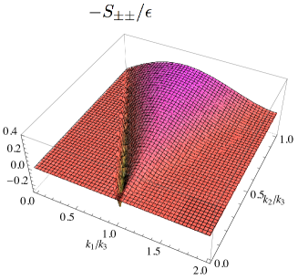
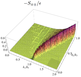
Figure 1: Shape function $S_{\pm\pm}(k_{1},k_{2},k_{3})$ for $c_{\gamma}=0.8$

Figure 2: Shape function $S_{\pm\mp}(k_{1},k_{2},k_{3})$ for $c_{\gamma}=0.8$

.7 On scalar bispectrum

Finally, we make a brief comment on scalar bispectra induced by the modified tensor sound speed. As in (28), the $\delta K_{\mu}^{\nu}\delta K_{\nu}^{\mu}$ operator induces cubic interactions of $\pi$, which can be a source of large scalar non-Gaussianities. Indeed, if $\delta K_{\mu}^{\nu}\delta K_{\nu}^{\mu}$ is the only relevant operator and other operators do not come into the game, the scalar nonlinearity parameter $f_{\rm NL}$ can be estimated as

$$f_{\rm NL}\sim\mathcal{O}\big{(}(c_{\gamma}^{-2}-1)/\epsilon\big{)}\,.$$ (43)

Since it is enhanced by the inverse of the slow-roll parameter, one may think that the current null observation of scalar non-Gaussianities can constrain the tensor sound speed as $c_{\gamma}^{-2}-1\lesssim\epsilon$. However, as shown in Table 1, various operators can induce $\pi^{3}$-type interactions and the scalar non-Gaussianities can be easily reduced in the presence of other operators. For example, when the $\delta K^{2}$ operator is relevant and $\bar{M}_{2}^{2}=-\bar{M}_{3}^{2}$,

$$S=S_{0}-\frac{\bar{M}_{3}^{2}}{2}\int d^{4}x\sqrt{-g}\big{(}\delta K_{\mu}^{\nu}\delta K^{\mu}_{\nu}-\delta K^{2}\big{)}\,,$$ (44)

the cubic interactions of $\pi$ exactly cancel out in the decoupling limit. In fact, the generalized Galileon Deffayet:2011gz ; Horndeski:1974wa accommodates this type of combination in the action Gleyzes:2013ooa . Thus, additional symmetries or tunings may decrease the scalar non-Gaussianities. In this way, scalar bispectra depend on various operators and the information of the tensor sound speed is obscured. In contrast, the scalar-tensor-tensor bispectra are more sensitive to the tensor sound speed and can be a powerful tool to measure it.

.8 Conclusion

In this Letter, we investigated the relation between non-Gaussianities of primordial perturbations and the sound speed of tensor perturbations, based on the EFT approach. We found that the modification of the tensor sound speed induces a significant enhancement of the scalar-tensor-tensor cross bispectrum, rather than the tensor auto-bispectrum. This situation is in sharp contrast with the case of the curvature perturbations, in which their auto-bispectra are significantly enhanced by their reduced sound velocity. When the sound speed of tensor perturbations is reduced, the scalar-tensor-tensor bispectrum is enhanced by a factor of $(c_{\gamma}^{-2}-1)/\epsilon$ compared to the case of $c_{\gamma}=1$ and such an enhancement makes it easy to detect the CMB bispectra of two B-modes and one temperature (or one E-mode) anisotropies especially. Thus, the scalar-tensor-tensor bispectrum and its relevant bispectra of the CMB can be powerful probes for the reduced tensor sound speed and the gravitational structure for inflation.

Acknowledgments

The work of T.N. is supported in part by the Special Postdoctoral Researcher Program at RIKEN. The work of M.Y. is supported in part by the JSPS Grant-in-Aid for Scientific Research on Innovative Areas No. 24111706 and the JSPS Grant-in-Aid for Scientific Research No. 25287054.

References

- (1) A. A. Starobinsky, Phys. Lett. B 91, 99 (1980). A. H. Guth, Phys. Rev. D 23, 347 (1981); K. Sato, Mon. Not. Roy. Astron. Soc. 195, 467 (1981).
- (2) D. Seery and J. E. Lidsey, JCAP 0506, 003 (2005) [astro-ph/0503692].
- (3) X. Chen, M. -x. Huang, S. Kachru and G. Shiu, JCAP 0701, 002 (2007) [hep-th/0605045].
- (4) P. A. R. Ade et al. [Planck Collaboration], arXiv:1303.5084 [astro-ph.CO].
- (5) J. M. Maldacena, JHEP 0305, 013 (2003) [astro-ph/0210603].
- (6) P. Creminelli and M. Zaldarriaga, JCAP 0410, 006 (2004) [astro-ph/0407059].
- (7) M. H. Namjoo, H. Firouzjahi and M. Sasaki, Europhys. Lett. 101, 39001 (2013) [arXiv:1210.3692 [astro-ph.CO]].
- (8) A. A. Starobinsky, JETP Lett. 30, 682 (1979) [Pisma Zh. Eksp. Teor. Fiz. 30, 719 (1979)].
- (9) P. A. R. Ade et al. [BICEP2 Collaboration], arXiv:1403.3985 [astro-ph.CO].
- (10) P. A. R. Ade et al. [Planck Collaboration], arXiv:1303.5082 [astro-ph.CO].
- (11) X. Gao, T. Kobayashi, M. Yamaguchi and J. ’i. Yokoyama, Phys. Rev. Lett. 107, 211301 (2011) [arXiv:1108.3513 [astro-ph.CO]].
- (12) T. Kobayashi, M. Yamaguchi and J. ’i. Yokoyama, Prog. Theor. Phys. 126, 511 (2011) [arXiv:1105.5723 [hep-th]].
- (13) C. Cheung, P. Creminelli, A. L. Fitzpatrick, J. Kaplan and L. Senatore, JHEP 0803, 014 (2008) [arXiv:0709.0293 [hep-th]].
- (14) T. Noumi and M. Yamaguchi, in preparation.
- (15) X. Gao, T. Kobayashi, M. Shiraishi, M. Yamaguchi, J. ’i. Yokoyama and S. Yokoyama, PTEP 2013, 053E03 (2013) [arXiv:1207.0588 [astro-ph.CO]].
- (16) C. Deffayet, X. Gao, D. A. Steer and G. Zahariade, Phys. Rev. D 84, 064039 (2011) [arXiv:1103.3260 [hep-th]].
- (17) G. W. Horndeski, Int. J. Theor. Phys. 10, 363 (1974).
- (18) J. Gleyzes, D. Langlois, F. Piazza and F. Vernizzi, JCAP 1308, 025 (2013) [arXiv:1304.4840 [hep-th]].