Gaia photometry for white dwarfs

Abstract

Context. White dwarfs can be used to study the structure and evolution of the Galaxy by analysing their luminosity function and initial mass function. Among them, the very cool white dwarfs provide the information for the early ages of each population. Because white dwarfs are intrinsically faint only the nearby ($\sim 20$ pc) sample is reasonably complete. The Gaia space mission will drastically increase the sample of known white dwarfs through its 5–6 years survey of the whole sky up to magnitude $V=20$–$25$.

Aims. We provide a characterisation of Gaia photometry for white dwarfs to better prepare for the analysis of the scientific output of the mission. Transformations between some of the most common photometric systems and Gaia passbands are derived. We also give estimates of the number of white dwarfs of the different galactic populations that will be observed.

Methods. Using synthetic spectral energy distributions and the most recent Gaia transmission curves, we computed colours of three different types of white dwarfs (pure hydrogen, pure helium, and mixed composition with H/He$=0.1$). With these colours we derived transformations to other common photometric systems (Johnson-Cousins, Sloan Digital Sky Survey, and 2MASS). We also present numbers of white dwarfs predicted to be observed by Gaia.

Results. We provide relationships and colour-colour diagrams among different photometric systems to allow the prediction and/or study of the Gaia white dwarf colours. We also include estimates of the number of sources expected in every galactic population and with a maximum parallax error. Gaia will increase the sample of known white dwarfs tenfold to about 200 000. Gaia will be able to observe thousands of very cool white dwarfs for the first time, which will greatly improve our understanding of these stars and early phases of star formation in our Galaxy.

1 Introduction

White dwarfs (WDs) are the final remnants of low- and intermediate-mass stars. About 95% of the main-sequence (MS) stars will end their evolutionary pathways as WDs and, hence, the study of the WD population provides details about the late stages of the life of the vast majority of stars. Their evolution can be described as a simple cooling process, which is reasonably well understood (Salaris et al. 2000; Fontaine et al. 2001). WDs are very useful objects to understand the structure and evolution of the Galaxy because they have an imprinted memory of its history (Isern et al. 2001; Liebert et al. 2005). The WD luminosity function (LF) gives the number of WDs per unit volume and per bolometric magnitude (Winget et al. 1987; Isern et al. 1998). From a comparison of observational data with theoretical LFs important information on the Galaxy (Winget et al. 1987) can be obtained (for instance, the age of the Galaxy, or the star formation rate). Moreover, the initial mass function (IMF) can be reconstructed from the LF of the relic WD population, that is, the halo/thick disc populations. The oldest members of these populations are cool high-mass WDs, which form from high-mass progenitors that evolved very quickly to the WD stage.

Because most WDs are intrinsically faint, it is difficult to detect them, and a complete sample is currently only available at very close distances. Holberg et al. (2008) presented a (probably) complete sample of local WDs within 13 pc and demonstrated that the sample becomes incomplete beyond that distance. More recently, Giammichele et al. (2012) provided a nearly complete sample up to 20 pc. Completeness of WD samples beyond 20 pc is still very unsatisfactory even though the number of known WDs has considerably increased thanks to several surveys. For instance, the Sloan Digital Sky Survey (SDSS), with a limiting magnitude of $g^{\prime}=19.5$ (Fukugita et al. 1996) and covering a quarter of the sky, has substantially increased the number of spectroscopically confirmed WDs. This has allowed several statistical studies (Eisenstein et al. 2006), and the consequent improvement of the WD LF and WD mass distribution (Kleinman et al. 2013; Tremblay et al. 2011; Krzesinski et al. 2009; De Gennaro et al. 2008; Hu et al. 2007; Harris et al. 2006). However, the number of very cool WDs and known members of the halo population is still very low. A shortfall in the number of WDs below $\log(L/L_{\odot})=-4.5$ because of the finite age of the Galactic disc, called luminosity cut-off, was first observed in the eighties (e.g. Liebert 1980; Winget et al. 1987). The Gaia mission will be extremely helpful in detecting WDs close to the luminosity cut-off and even fainter, which is expected to improve the accuracy of the age determined from the WD LF.

Gaia is the successor of the ESA Hipparcos astrometric mission (Bonnet et al. 1997) and increases its capabilities drastically, both in precision and in number of observed sources, offering the opportunity to tackle many open questions about the Galaxy (its formation and evolution, as well as stellar physics). Gaia will determine positions, parallaxes, and proper motions for a relevant fraction of stars ($10^{9}$ stars, $\sim 1\%$ of the Galaxy). This census will be complete for the full sky up to $V=20-25$ mag (depending on the spectral type) with unprecedented accuracy (Perryman et al. 2001, Prusti 2011). Photometry and spectrophotometry will be obtained for all the detected sources, while radial velocities will be obtained for the brightest ones (brighter than about 17^th magnitude). Each object in the sky will transit the focal plane about 70 times on average.

The Gaia payload consists of three instruments mounted on a single optical bench: the astrometric instrument, the spectrophotometers, and one high-resolution spectrograph. The astrometric measurements will be unfiltered to obtain the highest possible signal-to-noise ratio. The mirror coatings and CCD quantum efficiency define a broad (white-light) passband named $G$ (Jordi et al. 2010). The basic shape of the spectral energy distribution (SED) of every source will be obtained by the spectrophotometric instrument, which will provide low-resolution spectra in the blue (330–680 nm) and red (640–1000 nm), BP and RP spectrophotometers, respectively (see Jordi et al. 2010, for a detailed description). The BP and RP spectral resolutions are a function of wavelength. The dispersion is higher at short wavelengths. Radial velocities will also be obtained for more than 100 million stars through Doppler-shift measurements from high-resolution spectra ($R\sim 5000$–$11\,000$) obtained in the region of the IR Ca triplet around 860 nm by the Radial Velocity Spectrometer (RVS). Unfortunately, most WDs will show only featureless spectra in this region. The only exception are rare subtypes that display metal lines or molecular carbon bands (DZ, DQ, and similar).

The precision of the astrometric and photometric measurements will depend on the brightness and spectral type of the stars. At $G=15$ mag the end-of-mission precision in parallaxes will be $\sim 25$ $\mu$as. At $G=20$ mag the final precision will drop to $\sim 300$ $\mu$as, while for the brightest stars ($6<G<12$ mag) it will be $\sim 10$ $\mu$as. The end-of-mission $G$-photometric performance will be at the level of millimagnitudes. For radial velocities the precisions will be in the range 1 to 15 km s^-1 depending on the brightness and spectral type of the stars (Katz et al. 2011). For a detailed description of performances see the Gaia website.

An effective exploitation of this information requires a clear understanding of the potentials and limitations of Gaia data. This paper aims to provide information to researchers on the WD field to obtain the maximum scientific gain from the Gaia mission.

Jordi et al. (2010) presented broad Gaia passbands and colour-colour relationships for MS and giant stars, allowing the prediction of Gaia magnitudes and uncertainties from Johnson-Cousins (Bessell 1990) and/or SDSS (Fukugita et al. 1996) colours. That article used the BaSeL-3.1 (Westera et al. 2002) stellar spectral library, which includes SEDs with $-1.0<\log g<5.5$, and thus excluded the WD regime ($7.0<\log g<9.0$). The aim of the present paper is to provide a similar tool for characterizing Gaia observations of WDs. For that purpose, we used the most recent WD synthetic SEDs (Kilic et al. 2009b, 2010a; Tremblay et al. 2011; Bergeron et al. 2011, see Sect. 2) with different compositions to simulate Gaia observations. In Sect. 3 we describe the conditions of WD observations by Gaia (the obtained Gaia spectrophotometry, the WD limiting distances, expected error in their parallaxes, etc.). In Sect. 4 we provide the colour-colour transformations between Gaia passbands and other commonly used photometric systems like the Johnson-Cousins (Bessell 1990), SDSS (Fukugita et al. 1996), and 2MASS (Cohen et al. 2003). In Sect. 5 relationships among Gaia photometry and atmospheric parameters are provided. Estimates of the number of WDs that Gaia will potentially observe based on simulations by Napiwotzki (2009) and Gaia Universe Model Snapshot (GUMS, Robin et al. 2012) are provided in Sect. 6. Finally, in Sect. 7 we finish with a summary and conclusions.

2 Model atmospheres

To represent the SED of WDs, we used grids of pure hydrogen (pure-H), pure helium (pure-He), and also mixed-composition models (H/He$=0.1$) with $7.0<\log g<9.0$ in steps of $0.5$ dex. These SEDs were computed from state-of-the-art model atmospheres and were verified in recent photometric and spectral analyses of WDs (Kilic et al. 2009b, 2010a; Tremblay et al. 2011; Bergeron et al. 2011).

The pure-H models are drawn from Tremblay et al. (2011) and cover the range of $1500$ K $<$ $T_{\mathrm{eff}}$ $<140\,000$ K. These models were recently improved in the cool-temperature regime with updated collision-induced absorption (CIA) opacities (see the discussion in Tremblay & Bergeron 2007). In the present paper we also account for the opacity generated by the red wing of Lyman-$\alpha$ computed by Kowalski & Saumon (2006). This opacity significantly changes the predicted flux in the $B$ passband at very cool temperatures ($T_{\mathrm{eff}}$ $\lesssim 6000$ K). Models with this opacity source have been successful in reproducing SEDs of many cool WDs (Kowalski & Saumon 2006; Kilic et al. 2009a, b, 2010b; Durant et al. 2012). The colours for these improved models are accessible from Pierre Bergeron’s webpage. In Fig. 1, we compare the predicted spectra of cool ($4000$ K) pure-H atmosphere WDs using the former grid of Tremblay et al. (2011) with the present grid taking into account the Lyman-$\alpha$ opacity.

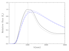
Figure 1: Comparison of model SEDs with $T_{\mathrm{eff}}$ $=4000$ K and $\log g=8.0$. The pure-H models (in black) are computed with and without the Lyman-$\alpha$ opacity (solid and dotted lines). The pure-He models (in blue) are drawn from the sequence using the equation of state of Bergeron et al. (1995) and using the improved high-density physics of Kowalski et al. 2007 (medium and long dashed lines). The dotted vertical lines show the limits where the Gaia transmission is higher than 5%.

We additionally used pure-He models drawn from Bergeron et al. (2011), which cover a range of $3500$ K $<$ $T_{\mathrm{eff}}$ $<40\,000$ K. The cooler pure-He DC models are described in more detail in Kilic et al. (2010a), and their main feature is the non-ideal equation of state of Bergeron et al. (1995). In recent years, new pure-He models of Kowalski et al. (2007), which include improved description of non-ideal physics and chemistry of dense helium, have also been used in the analysis of the data (Kilic et al. 2009b). These models include a number of improvements in the description of pure-He atmospheres of very cool WDs. These include refraction (Kowalski & Saumon 2004), non-ideal chemical abundances of species, and improved models of Rayleigh scattering and He^- free-free opacity (Iglesias et al. 2002; Kowalski et al. 2007). The SEDs of pure-He atmospheres are close to those of black bodies, since the He^- free-free opacity, which has a low dependence on wavelength, becomes the dominant opacity source in these models. In Fig. 1, we also present models at $4000$ K drawn from the two pure-He sequences. The blue flux in Kowalski et al. (2007) is slightly higher than in Bergeron et al. (1995) since the contribution of the Rayleigh scattering is diminished. Note that the IR wavelength domain, which is not covered by Gaia detectors, is the range in which larger differences between the pure-H or pure-He composition are present. These differences result from strong CIA absorption by molecular hydrogen in hydrogen-dominated atmospheres.

Figure 2 shows that in spite of the different physics present in all these models, the colours (e.g. $G-V$) look quite similar for the different SED libraries. For this reason, and because the purpose of this paper is not to discuss the differences among the WD SED libraries, but to provide a way to predict how WDs will be observed by Gaia, in Sect. 4 we only included the transformations derived using one sequence for each composition (Tremblay et al. 2011 with Lyman-$\alpha$ for pure-H and Bergeron et al. 2011 for pure-He).

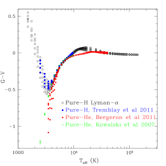
Figure 2: ($G-V$) vs. $T_{\mathrm{eff}}$ diagram for WD SEDs (red filled squares and black opened circles) compared with pure-H SEDs without the Lyman-$\alpha$ opacity (blue filled circles) and pure-He SEDs from Kowalski et al. 2007 (green star symbols).

The mixed model atmospheres used here cover a range of $2500$ K $<$ $T_{\mathrm{eff}}$ $<6000$ K and are taken from Kilic et al. (2010a). In the following, we use an abundance ratio of H/He $=0.1$ as a typical example for the composition of known mixed WDs (Kilic et al. 2009b, 2010a; Leggett et al. 2011; Giammichele et al. 2012). It has to be kept in mind that because of the nature of the CIA opacities, which are dominant in the near-IR and IR in this mixed regime, the predicted spectra can vary considerably for different H/He ratios with the same $T_{\mathrm{eff}}$ and $\log g$ (see Fig. 10 of Kilic et al. 2010a). The colour space covered by our H/He $=0.1$ sequence and the pure-H and He sequences illustrates the possible colour area where mixed-composition WDs can be found.

3 WDs as seen by Gaia

In Fig. 3 the synthetic SEDs of selected WDs (see Sect. 2) are shown together with the transmission curves of the $G$ passband, BP/RP spectrophotometry, and RVS spectroscopy. Low-resolution BP/RP spectra as will be obtained by Gaia for pure-H WDs are shown in Fig. 4. If these spectra are re-binned, summing all their pixels together, we obtain their corresponding magnitudes, $G_{\rm BP}$, $G_{\rm RP}$, and $G_{\rm RVS}$ (Fig. 3). In the same way, we can reproduce any other synthetic passband, if needed (e.g. Johnson-Cousins, SDSS, or 2MASS, etc.).

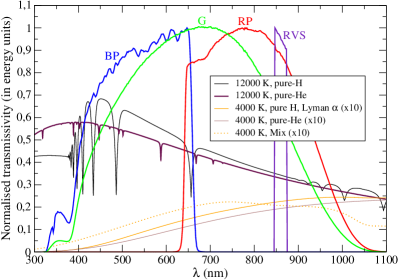
Figure 3: Gaia passbands transmissivity. $G$ passband is depicted in green, $G_{\rm BP}$ in blue, $G_{\rm RP}$ in red, and $G_{\rm RVS}$ in magenta lines. All WD SEDs plotted here (described in Sect. 2) correspond to $\log g=8.0$.

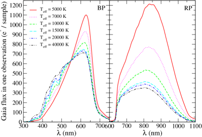
Figure 4: Examples of Gaia BP/RP spectra for pure-H WDs (Tremblay et al. 2011) with different temperatures at $G=15$ mag. All SEDs plotted here have $\log g=8.0$.

The faint Gaia limiting magnitude will guarantee the detection of very cool WDs. In Table 1 we compute the maximum distances at which WDs with different temperatures and gravities will be detected with Gaia. Two limiting distances are provided, without considering interstellar absorption, $d$, and assuming an average absorption of 1 mag per kpc, $d_{\rm A_{V}}$, corresponding to an observation made in the direction of the Galactic disc (O’Dell & Yusef-Zadeh 2000). We also provide the absolute magnitudes ($M_{G}$) and consider two different compositions, pure-H and pure-He. All WDs with $T_{\mathrm{eff}}$ $>20\,000$ K will be detected within $270$ pc and all with $T_{\mathrm{eff}}$ $>10\,000$ K within $150$ pc, regardless of the atmospheric composition or interstellar absorption. The brightest unreddened WDs will even be observed farther away than 1.5 kpc. For the coolest regime the space volume of observation is smaller, especially at high $\log g$, with detections restricted to the nearest 50 pc (for $T_{\mathrm{eff}}$ $=5000$ K).

Table 1: Maximum distances, $d$, at which unreddened WDs will be observed by Gaia for pure-H (Tremblay et al. 2011) and pure-He (Bergeron et al. 2011, which only covers $T_{\mathrm{eff}}$ $>3500$ K) models. $d_{\rm A_{V}}$ is the limiting distance when an average reddening corresponding to an observation in the disc direction has been applied (assuming an extinction of 1 mag$\cdot$kpc^-1). The ages of all these WDs can be consulted in the CDS online tables (Tables 3 – 5). $M_{G}$ is the absolute magnitude at $G$ passband.

	$\log g=7.0$			$\log g=8.0$			$\log g=9.0$
$T_{\mathrm{eff}}$	$M_{G}$	$d$ (pc)	$d_{\rm A_{V}}$ (pc)	$M_{G}$	$d$ (pc)	$d_{\rm A_{V}}$ (pc)	$M_{G}$	$d$ (pc)	$d_{\rm A_{V}}$ (pc)
Pure-H (Lyman-$\alpha$)
$2000$	$17.28$	$35$	$34$	$18.22$	$23$	$22$	$19.77$	$11$	$11$
$3000$	$15.80$	$69$	$67$	$16.76$	$45$	$44$	$18.38$	$21$	$21$
$4000$	$14.86$	$107$	$102$	$15.84$	$68$	$66$	$17.44$	$33$	$32$
$5000$	$13.72$	$180$	$167$	$14.86$	$107$	$102$	$16.55$	$49$	$48$
$10\,000$	$10.74$	$711$	$552$	$12.18$	$366$	$317$	$13.96$	$161$	$151$
$20\,000$	$9.23$	$1425$	$929$	$10.81$	$689$	$538$	$12.59$	$303$	$268$
Pure-He
$4000$	$15.16$	$93$	$89$	$16.09$	$61$	$59$	$17.77$	$28$	$27$
$5000$	$13.76$	$177$	$164$	$14.86$	$107$	$102$	$16.58$	$48$	$47$
$10\,000$	$10.92$	$655$	$516$	$12.28$	$350$	$304$	$14.02$	$157$	$147$
$20\,000$	$9.17$	$1465$	$947$	$10.68$	$731$	$564$	$12.44$	$325$	$285$

The Gaia photometry combined with its extremely precise parallaxes will allow absolute magnitudes to be derived, which will provide precise locations in the Hertzsprung–Russell (HR) diagrams (see Sect. 5). Estimates of the number of WDs observed by Gaia with a given parallax and a given relative error in the parallax are provided in Fig. 5 (left and right, respectively), based on simulations performed with GUMS, see Sect. 6. The errors in parallaxes were computed using Gaia performance prescriptions². Estimates derived from Fig. 5 of the number of WDs with better parallax precision than a certain threshold are provided in the upper part of Table 2. About 95% of the isolated WDs brighter than $G=20$ will have parallaxes more precise than 20%.

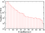
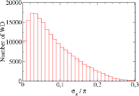
Figure 5: Histogram of parallaxes (left) of single WDs with $G\leq 20$ using data from GUMS. Histogram of parallax relative errors (right) computed using Gaia performances².

Table 2: Approximate number of WDs (all temperatures) with parallaxes better than a certain percentage, derived using the GUMS dataset and real WD SDSS datasets (extracted from Kilic et al. 2010a; Tremblay et al. 2011).

	GUMS
	All WDs		Single WDs
$\sigma_{\pi}$ / $\pi$	$N$	% of observed	$N$	% of observed
$\leq$1%	$20\,000$	3.5%	$10\,000$	5%
$\leq$5%	$150\,000$	25%	$75\,000$	40%
$\leq$10%	$300\,000$	50%	$135\,000$	70%
$\leq$20%	$450\,000$	80%	$190\,000$	95%
	WDs from SDSS samples
	Kilic et al. (2010a)		Tremblay et al. (2011)
$\sigma_{\pi}$ / $\pi$	$N$	% of observed	$N$	% of observed
$\leq$1%	76	61%	500	16%
$\leq$5%	125	100%	$2275$	74%
$\leq$10%	125	100%	$2880$	94%
$\leq$20%	125	100%	$3048$	99%

Expected end-of-mission parallax uncertainties were also computed for two observational datasets extracted from SDSS data. The first sample includes 125 cool ($T_{\mathrm{eff}}$ $<7000$ K) WDs analysed by Kilic et al. (2010a), the second data set includes almost $3000$ hot ($6000$ K $<$ $T_{\mathrm{eff}}$ $<140\,000$ K), non-magnetic and single WDs from Tremblay et al. (2011). The relative error of their parallaxes, derived from predicted distances, are shown in Fig. 6. For these samples, we computed the values quoted in the bottom part of Table 2. As can be seen, 94% of the WDs will have parallax determinations better than 10%, corresponding to absolute magnitudes with uncertainties below $0.2$ mag, which allows a clear distinction between WDs and MS stars. While the masses for the sample of Tremblay et al. (2011) are known from spectroscopic fits, the masses of the cool WDs from Kilic et al. (2010a) are not constrained, and therefore Gaia will be able to provide this information for the first time.

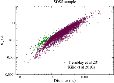
Figure 6: Relative error in Gaia parallax as a function of the distance for real WDs observed by SDSS, showing that Gaia will be precise enough to easily cover the $100$ pc WD sample at a $\sim 1$% level.

Gaia will also observe (and discover new) binaries containing WDs (according to simulations by GUMS shown in Table 9, only $36\%$ of WDs detected by Gaia will be single) and orbital solutions will be achieved for a significant number of them. Therefore, Gaia will provide independent mass determinations of WDs. These data are desirable to check and calibrate the currently available mass estimates of WDs based on the models and photometric/spectroscopic data. Among all these binaries, eclipsing binaries will be extremely useful to determine the radius of the WD. We currently know more than $2000$ binary pairs composed of a WD and an MS star (Rebassa-Mansergas et al. 2011). Only 34 systems of this sample are eclipsing binaries. About a thousand more will be discovered by Gaia.

4 Gaia photometric transformations

For each available WD SED in the libraries described in Sect. 2, we computed their Gaia photometry as they would be observed with Gaia and other commonly used photometric systems (Johnson-Cousins, SDSS and 2MASS) following the same strategy as Jordi et al. (2010). The results are listed in the CDS online Tables 3 – 5. The contents of these tables include the astrophysical parameters of the WDs (effective temperature, surface gravity, mass in solar masses, bolometric magnitude, bolometric correction in $V$, and age) as well as their simulated absolute magnitudes in Johnson-Cousins ($U$, $B$, $V$, $R_{C}$, $I_{C}$), 2MASS ($J$, $H$, $K_{S}$), SDSS ($u$, $g$, $r$ , $i$, $z$), and Gaia passbands ($G$, $G_{\rm BP}$, $G_{\rm RP}$, and $G_{\rm RVS}$). The three different tables correspond to different compositions of the WDs (pure-H in Table 3, pure-He in Table 4, and mixed composition with H/He=0.1 in Table 5).

Because WDs are intrinsically faint objects, they are observed close to us. Because of this, they are not much affected by extinction. For this reason, the colour transformations presented in this section were obtained without reddening effects, which are considered negligible for most WDs observed by Gaia. The hot WDs in the Galactic disc direction may, however, suffer from mild to considerable reddening, although this will have to be studied on a case-by-case basis, which is currently beyond the scope of this work.

3

Table 3: Gaia, Johnson, 2MASS, and SDSS absolute magnitudes derived for WD SEDs extracted from Tremblay et al. (2011) for pure-H composition WDs. Only the first records are shown. The full table is available at the CDS.

$T_{\mathrm{eff}}$	$\log g$	$M/M_{\odot}$	$M_{\rm bol}$	$BC_{V}$	$M_{U}$	$M_{B}$	$M_{V}$	$M_{R_{C}}$	$M_{I_{C}}$	$M_{J}$	$M_{H}$	$M_{K_{S}}$	$M_{u}$	$M_{g}$	$M_{r}$	$M_{i}$	$M_{z}$	$M_{y}$	$M_{G}$	$M_{\rm G_{\rm BP}}$	$M_{\rm G_{\rm RP}}$	$M_{\rm G_{\rm RVS}}$	Age
1500	7.0	0.150	19.064	1.043	22.926	20.527	18.021	17.746	19.438	19.578	19.584	21.336	23.940	19.241	17.619	19.668	19.352	17.980	18.380	18.414	18.660	19.037	1.623E+10
1750	7.0	0.151	18.393	0.787	22.232	20.018	17.607	17.153	18.233	18.418	18.556	19.798	23.228	18.800	17.070	18.526	18.313	17.583	17.779	17.933	17.705	17.888	1.338E+10
2000	7.0	0.151	17.812	0.524	21.626	19.588	17.288	16.687	17.240	17.456	17.705	18.621	22.599	18.437	16.673	17.580	17.441	17.273	17.275	17.575	16.924	16.946	1.078E+10
2250	7.0	0.151	17.297	0.281	21.083	19.203	17.016	16.299	16.427	16.651	16.968	17.633	22.038	18.113	16.368	16.807	16.712	17.003	16.830	17.284	16.277	16.176	7.879E+09
2500	7.0	0.152	16.837	0.059	20.590	18.855	16.778	15.974	15.757	15.963	16.330	16.817	21.529	17.822	16.128	16.191	16.094	16.764	16.440	17.039	15.740	15.538	5.479E+09
2750	7.0	0.152	16.420	-0.136	20.123	18.526	16.556	15.696	15.220	15.353	15.742	16.103	21.046	17.546	15.922	15.710	15.578	16.541	16.099	16.816	15.297	15.019	3.943E+09
3000	7.0	0.152	16.039	-0.295	19.654	18.195	16.334	15.451	14.807	14.794	15.173	15.439	20.563	17.269	15.727	15.342	15.158	16.318	15.802	16.596	14.939	14.613	3.472E+09
.
.
.

4

Table 4: Gaia, Johnson-Cousins, 2MASS, and SDSS absolute magnitudes derived for WD SEDs extracted from Bergeron et al. (2011) for pure-He composition WDs. Only the first records are shown. The full table is available at the CDS.

$T_{\mathrm{eff}}$	$\log g$	$M/M_{\odot}$	$M_{\rm bol}$	$BC_{V}$	$M_{U}$	$M_{B}$	$M_{V}$	$M_{R_{C}}$	$M_{I_{C}}$	$M_{J}$	$M_{H}$	$M_{K_{S}}$	$M_{u}$	$M_{g}$	$M_{r}$	$M_{i}$	$M_{z}$	$M_{y}$	$M_{G}$	$M_{\rm G_{\rm BP}}$	$M_{\rm G_{\rm RP}}$	$M_{\rm G_{\rm RVS}}$	Age
3500	7.0	0.150	15.387	-1.803	20.374	19.186	17.190	15.907	14.774	13.610	13.120	12.831	21.252	18.245	16.371	15.474	14.944	17.202	16.104	17.371	14.980	14.508	2.902E+09
3750	7.0	0.151	15.083	-1.432	19.367	18.340	16.515	15.371	14.352	13.350	12.921	12.670	20.235	17.475	15.785	15.008	14.569	16.517	15.605	16.720	14.546	14.114	2.792E+09
4000	7.0	0.151	14.797	-1.115	18.449	17.573	15.912	14.895	13.983	13.124	12.748	12.527	19.308	16.779	15.264	14.600	14.243	15.906	15.155	16.134	14.164	13.772	2.489E+09
4250	7.0	0.152	14.526	-0.845	17.605	16.874	15.371	14.473	13.662	12.928	12.596	12.402	18.455	16.148	14.804	14.244	13.960	15.360	14.750	15.604	13.829	13.475	2.193E+09
4500	7.0	0.153	14.271	-0.617	16.818	16.233	14.888	14.100	13.384	12.758	12.464	12.293	17.662	15.575	14.398	13.934	13.715	14.872	14.384	15.125	13.535	13.218	1.955E+09
4750	7.0	0.155	14.026	-0.431	16.079	15.644	14.457	13.772	13.142	12.611	12.349	12.197	16.916	15.053	14.040	13.664	13.502	14.438	14.054	14.691	13.278	12.995	1.737E+09
5000	7.0	0.157	13.791	-0.286	15.385	15.108	14.077	13.484	12.932	12.480	12.245	12.110	16.215	14.584	13.728	13.430	13.317	14.058	13.757	14.300	13.055	12.802	1.546E+09
.
.
.

5

Table 5: Gaia, Johnson-Cousins, 2MASS, and SDSS absolute magnitudes derived for WD SEDs extracted from Kilic et al. (2010a) for mixed (He/H$=0.1$) composition WDs. Only the first records are shown. The full table is available at the CDS.

$T_{\mathrm{eff}}$	$\log g$	$M/M_{\odot}$	$M_{\rm bol}$	$BC_{V}$	$M_{U}$	$M_{B}$	$M_{V}$	$M_{R_{C}}$	$M_{I_{C}}$	$M_{J}$	$M_{H}$	$M_{K_{S}}$	$M_{u}$	$M_{g}$	$M_{r}$	$M_{i}$	$M_{z}$	$M_{y}$	$M_{G}$	$M_{\rm G_{\rm BP}}$	$M_{\rm G_{\rm RP}}$	$M_{\rm G_{\rm RVS}}$	Age
2000	7.0	0.147	17.840	1.023	18.395	17.917	16.817	17.047	18.728	19.978	21.054	23.900	19.233	17.308	16.982	18.455	19.574	16.741	17.307	17.207	18.037	19.059	1.017E+10
2250	7.0	0.147	17.331	0.894	17.960	17.561	16.437	16.392	17.764	18.949	20.028	22.339	18.794	16.974	16.351	17.550	18.563	16.387	16.771	16.762	17.113	18.016	9.629E+09
2500	7.0	0.147	16.874	0.749	17.566	17.239	16.125	15.870	16.862	18.002	19.086	20.968	18.398	16.674	15.886	16.675	17.649	16.091	16.299	16.400	16.323	17.096	8.280E+09
2750	7.0	0.147	16.454	0.598	17.206	16.944	15.856	15.449	16.008	17.115	18.183	19.570	18.036	16.399	15.535	15.927	16.830	15.832	15.880	16.100	15.664	16.262	4.873E+09
3000	7.0	0.148	16.068	0.441	16.884	16.681	15.627	15.126	15.300	16.357	17.403	18.354	17.712	16.156	15.270	15.379	16.057	15.608	15.530	15.852	15.140	15.484	3.673E+09
3250	7.0	0.149	15.714	0.285	16.597	16.447	15.429	14.872	14.738	15.670	16.713	17.425	17.424	15.939	15.062	14.974	15.389	15.411	15.234	15.643	14.715	14.816	3.173E+09
3500	7.0	0.150	15.387	0.148	16.321	16.221	15.239	14.655	14.312	15.009	16.031	16.564	17.146	15.730	14.876	14.667	14.861	15.223	14.977	15.446	14.371	14.299	2.902E+09
.
.
.

4.1 Johnson-Cousins and SDSS colours

Figures 7–8 show several colour-colour diagrams relating Gaia, Johnson-Cousins (Bessell 1990), and SDSS passbands (Fukugita et al. 1996). Only ’normal’ pure-H ($T_{\mathrm{eff}}$ $>5000$ K) and pure-He composition WDs are plotted. In this range of $T_{\mathrm{eff}}$, colours of mixed composition WDs coincide with those of pure-H WDs and are not overplotted for clarity. The relationship among colours is tight for each composition, that is, independent of the gravities. However, the $B$ and to a lesser degree the $V$ passband induce a distinction between the pure-H and the pure-He WDs at $T_{\mathrm{eff}}$ $\sim 13\,000$ K, where the Balmer lines and the Balmer jump are strong in pure-H WDs.

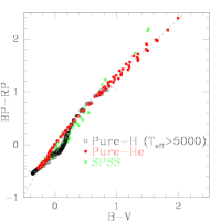
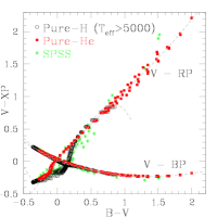
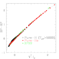
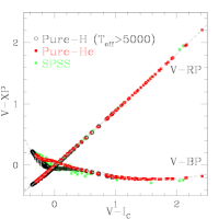
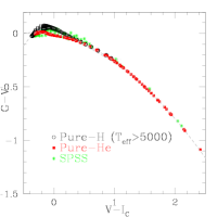
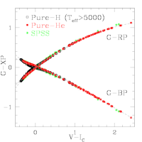
Figure 7: Several colour-colour diagrams obtained using Gaia and Johnson-Cousins passbands for the ’normal’ regime of pure-H ($T_{\mathrm{eff}}$ $>5000$ K; black open circles) and for pure-He (red squares) WDs. Green star symbols correspond to real WDs selected from Pancino et al. (2012). Grey dashed curves are the fitted polynomials from Table 6.

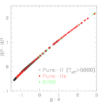
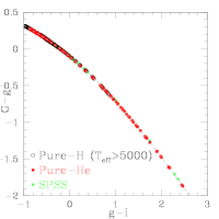
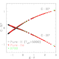
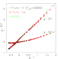
Figure 8: Same as Fig. 7, but for SDSS colours.

Synthetic photometry was also computed for 82 real WDs extracted from the list of Pancino et al. (2012). They are SpectroPhotometric Standard Star (SPSS) candidates for the absolute flux calibration of Gaia photometric and spectrophotometric observations. The whole list of SPSS is selected from calibration sources already used as flux standards for HST (Bohlin 2007), some sources from CALSPEC standards (Oke 1990, Hamuy et al. 1992, Hamuy et al. 1994, Stritzinger et al. 2005), and finally McCook & Sion (1999) but also SDSS, and other sources. The colours computed with the SEDs of the libraries used here (Sect. 2) agree very well with those of SPSS true WDs.

Because of the very tight relationship among colours, polynomial expressions were fitted. 240 synthetic pure-He and 276 synthetic pure-H WDs were used for the fitting. We provide the coefficients for third-order polynomials and the dispersion values in Table 6 (available online). Table 6 contains the following information. Column 1 lists the name of the source, Column 2 gives the bolometric luminosity, etc.

The dispersions are smaller than 0.02 mag for the SDSS passbands, while for the Johnson-Cousins passbands they can reach 0.06 mag in some case, mainly for pure-H and when blue $B$ or $G_{\rm BP}$ passbands are involved. The expressions presented here are useful to predict Gaia magnitudes for WDs of different $T_{\mathrm{eff}}$ and atmospheric compositions, for which colours in the Johnson-Cousins photometric system are known. These expressions should only be used in the $T_{\mathrm{eff}}$ regimes indicated in Table 6. In all other cases, individual values from the CDS online Tables 3–5 can be used instead.

In the cool regime, $T_{\mathrm{eff}}$ $<5000$ K, and for pure-H composition the colours depend considerably on the surface gravity, yielding a spread in the colour-colour diagrams (see Figs. 9 and 10). Therefore, no attempt has been made to include these cool pure-H WDs into the computation of the polynomial transformations. To derive the Gaia magnitudes, we recommend the use of the individual values for the desired temperature and surface gravity listed in the CDS online Tables 3 – 5.

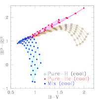
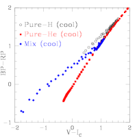
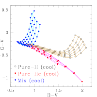
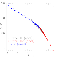
Figure 9: Several colour-colour diagrams obtained using Gaia and Johnson-Cousins passbands in the cool regime ($T_{\mathrm{eff}}$ $<5000$ K).

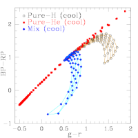
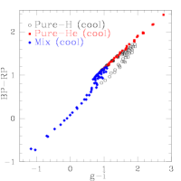
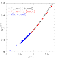
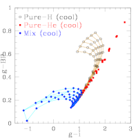
Figure 10: Same as Fig. 9, but for SDSS passbands.

6

Table 6: Coefficients of the colour-colour polynomial fittings using the Johnson-Cousins and SDSS passbands.

Johnson-Cousins						SDSS
Pure-H ($T_{\mathrm{eff}}$ $>5000$ K)
Colour	Zero point	$V-I_{C}$	$(V-I_{C})^{2}$	$(V-I_{C})^{3}$	$\sigma$	Colour	Zero point	$g-i$	$(g-i)^{2}$	$(g-i)^{3}$	$\sigma$
$G-$$G_{\rm BP}$	-0.0106	-0.4093	0.3189	-0.3699	0.009	$G-$$G_{\rm BP}$	-0.1186	-0.3188	-0.0276	-0.0390	0.007
$G-$$G_{\rm RP}$	0.0187	0.7797	-0.4716	0.3166	0.009	$G-$$G_{\rm RP}$	0.2214	0.5655	-0.0756	-0.0596	0.008
$G-$$G_{\rm RVS}$	0.0517	1.0443	-0.6142	0.4035	0.013	$G-$$G_{\rm RVS}$	0.3246	0.7604	-0.1031	-0.0871	0.009
$G_{\rm BP}$-$G_{\rm RP}$	0.0292	1.1890	-0.7905	0.6865	0.019	$G_{\rm BP}$-$G_{\rm RP}$	0.3400	0.8843	-0.0480	-0.0206	0.013
$G-V$	0.0495	-0.0907	-0.6233	0.4240	0.013	$G-g$	-0.1020	-0.5132	-0.0980	-0.0077	0.003
$V-$$G_{\rm RVS}$	0.0022	1.1350	0.0091	-0.0205	0.001	$g-$$G_{\rm RVS}$	0.4266	1.2736	-0.0051	-0.0794	0.007
$V-$$G_{\rm BP}$	-0.0601	-0.3186	0.9421	-0.7939	0.021	$g-$$G_{\rm BP}$	-0.0166	0.1943	0.0704	-0.0313	0.009
$V-$$G_{\rm RP}$	-0.0308	0.8704	0.1516	-0.1073	0.004	$g-$$G_{\rm RP}$	0.3234	1.0787	0.0224	-0.0519	0.005
Color	Zero point	$V-R$	$(V-R)^{2}$	$(V-R)^{3}$	$\sigma$	Colour	Zero point	$g-r$	$(g-r)^{2}$	$(g-r)^{3}$	$\sigma$
$G-$$G_{\rm BP}$	-0.0232	-0.9322	1.9936	-3.8732	0.015	$G-$$G_{\rm BP}$	-0.0891	-0.5172	-0.0306	-0.0206	0.007
$G-$$G_{\rm RP}$	0.0427	1.7388	-3.2195	4.3387	0.019	$G-$$G_{\rm RP}$	0.1658	0.9376	-0.1314	-0.3685	0.011
$G-$$G_{\rm RVS}$	0.0838	2.3270	-4.2247	5.6185	0.026	$G-$$G_{\rm RVS}$	0.2498	1.2602	-0.1749	-0.5183	0.014
$G_{\rm BP}$-$G_{\rm RP}$	0.0659	2.6710	-5.2132	8.2118	0.034	$G_{\rm BP}$-$G_{\rm RP}$	0.2550	1.4548	-0.1008	-0.3480	0.016
$G-V$	0.0473	-0.1712	-2.8314	4.0591	0.017	$G-g$	-0.0555	-0.8062	-0.2123	0.1398	0.003
$V-$$G_{\rm RVS}$	0.0366	2.4982	-1.3933	1.5594	0.010	$g-$$G_{\rm RVS}$	0.3053	2.0664	0.0374	-0.6581	0.015
$V-$$G_{\rm BP}$	-0.0704	-0.7610	4.8250	-7.9323	0.032	$g-$$G_{\rm BP}$	-0.0336	0.2889	0.1817	-0.1604	0.009
$V-$$G_{\rm RP}$	-0.0045	1.9100	-0.3881	0.2796	0.003	$g-$$G_{\rm RP}$	0.2214	1.7438	0.0809	-0.5083	0.011
Colour	Zero point	$R-I$	$(R-I)^{2}$	$(R-I)^{3}$	$\sigma$	Colour	Zero point	$r-i$	$(r-i)^{2}$	$(r-i)^{3}$	$\sigma$
$G-$$G_{\rm BP}$	0.0002	-0.7288	0.7736	-2.3657	0.007	$G-$$G_{\rm BP}$	-0.1647	-0.8976	-0.9866	-2.5767	0.008
$G-$$G_{\rm RP}$	-0.0015	1.4227	-0.9942	1.4162	0.006	$G-$$G_{\rm RP}$	0.3038	1.4093	-0.2031	0.8241	0.008
$G-$$G_{\rm RVS}$	0.0247	1.9071	-1.2742	1.7530	0.007	$G-$$G_{\rm RVS}$	0.4355	1.8921	-0.3275	0.9117	0.008
$G_{\rm BP}$-$G_{\rm RP}$	-0.0017	2.1515	-1.7679	3.7820	0.013	$G_{\rm BP}$-$G_{\rm RP}$	0.4685	2.3069	0.7835	3.4008	0.015
$G-V$	0.0509	-0.1835	-2.1595	2.7057	0.010	$G-g$	-0.1796	-1.5031	-1.6721	-2.4821	0.009
$V-$$G_{\rm RVS}$	-0.0262	2.0906	0.8853	-0.9527	0.007	$g-$$G_{\rm RVS}$	0.6150	3.3952	1.3446	3.3938	0.012
$V-$$G_{\rm BP}$	-0.0507	-0.5453	2.9331	-5.0714	0.015	$g-$$G_{\rm BP}$	0.0149	0.6055	0.6855	-0.0945	0.010
$V-$$G_{\rm RP}$	-0.0524	1.6062	1.1653	-1.2894	0.009	$g-$$G_{\rm RP}$	0.4834	2.9124	1.4690	3.3062	0.012
Colour	Zero point	$B-V$	$(B-V)^{2}$	$(B-V)^{3}$	$\sigma$	Colour	Zero point	$g-z$	$(g-z)^{2}$	$(g-z)^{3}$	$\sigma$
$G-$$G_{\rm BP}$	0.0700	-0.5674	-0.4765	0.4891	0.015	$G-$$G_{\rm BP}$	-0.1488	-0.2450	-0.0313	-0.0325	0.006
$G-$$G_{\rm RP}$	-0.1251	1.0288	0.8762	-1.2221	0.033	$G-$$G_{\rm RP}$	0.2756	0.4128	-0.0513	-0.0099	0.004
$G-$$G_{\rm RVS}$	-0.1404	1.3779	1.1891	-1.6605	0.044	$G-$$G_{\rm RVS}$	0.3973	0.5549	-0.0713	-0.0170	0.004
$G_{\rm BP}$-$G_{\rm RP}$	-0.1951	1.5962	1.3527	-1.7112	0.047	$G_{\rm BP}$-$G_{\rm RP}$	0.4244	0.6579	-0.0201	0.0226	0.008
$G-V$	0.0607	-0.1378	-0.8979	0.7349	0.020	$G-g$	-0.1508	-0.4044	-0.0731	-0.0219	0.006
$V-$$G_{\rm RVS}$	-0.2011	1.5157	2.0870	-2.3954	0.063	$g-$$G_{\rm RVS}$	0.5481	0.9593	0.0018	0.0049	0.002
$V-$$G_{\rm BP}$	0.0093	-0.4297	0.4214	-0.2458	0.006	$g-$$G_{\rm BP}$	0.0020	0.1594	0.0418	-0.0106	0.010
$V-$$G_{\rm RP}$	-0.1858	1.1666	1.7741	-1.9570	0.052	$g-$$G_{\rm RP}$	0.4264	0.8173	0.0217	0.0120	0.003
Pure-He (All $T_{\mathrm{eff}}$)
Colour	Zero point	$V-I_{C}$	$(V-I_{C})^{2}$	$(V-I_{C})^{3}$	$\sigma$	Colour	Zero point	$g-i$	$(g-i)^{2}$	$(g-i)^{3}$	$\sigma$
$G-$$G_{\rm BP}$	0.0372	-0.4155	-0.0864	0.0149	0.005	$G-$$G_{\rm BP}$	-0.1127	-0.3463	-0.0320	0.0028	0.004
$G-$$G_{\rm RP}$	-0.0166	0.7803	-0.1451	0.0067	0.004	$G-$$G_{\rm RP}$	0.2307	0.5106	-0.0860	0.0063	0.004
$G-$$G_{\rm RVS}$	-0.0076	1.0204	-0.1584	0.0035	0.006	$G-$$G_{\rm RVS}$	0.3194	0.6817	-0.0984	0.0063	0.008
$G_{\rm BP}$-$G_{\rm RP}$	-0.0538	1.1958	-0.0587	-0.0082	0.009	$G_{\rm BP}$-$G_{\rm RP}$	0.3434	0.8568	-0.0539	0.0034	0.007
$G-V$	-0.0085	-0.1051	-0.1541	0.0046	0.006	$G-g$	-0.1051	-0.5219	-0.0949	0.0065	0.001
$V-$$G_{\rm RVS}$	0.0009	1.1255	-0.0043	-0.0011	0.002	$g-$$G_{\rm RVS}$	0.4244	1.2036	-0.0035	-0.0002	0.007
$V-$$G_{\rm BP}$	0.0456	-0.3104	0.0676	0.0103	0.010	$g-$$G_{\rm BP}$	-0.0076	0.1756	0.0629	-0.0036	0.004
$V-$$G_{\rm RP}$	-0.0082	0.8854	0.0089	0.0021	0.003	$g-$$G_{\rm RP}$	0.3358	1.0324	0.0090	-0.0002	0.003
Colour	Zero point	$V-R$	$(V-R)^{2}$	$(V-R)^{3}$	$\sigma$	Colour	Zero point	$g-r$	$(g-r)^{2}$	$(g-r)^{3}$	$\sigma$
$G-$$G_{\rm BP}$	0.0410	-0.8360	-0.3441	0.1642	0.006	$G-$$G_{\rm BP}$	-0.0758	-0.5153	-0.0698	0.0054	0.007
$G-$$G_{\rm RP}$	-0.0238	1.5787	-0.6202	0.0600	0.010	$G-$$G_{\rm RP}$	0.1743	0.8064	-0.2102	0.0258	0.007
$G-$$G_{\rm RVS}$	-0.0169	2.0629	-0.6808	0.0292	0.015	$G-$$G_{\rm RVS}$	0.2443	1.0710	-0.2412	0.0271	0.012
$G_{\rm BP}$-$G_{\rm RP}$	-0.0647	2.4147	-0.2761	-0.1042	0.016	$G_{\rm BP}$-$G_{\rm RP}$	0.2501	1.3217	-0.1403	0.0204	0.013
$G-V$	-0.0073	-0.2094	-0.6447	0.1165	0.006	$G-g$	-0.0500	-0.7598	-0.2141	0.0145	0.006
$V-$$G_{\rm RVS}$	-0.0096	2.2723	-0.0361	-0.0873	0.013	$g-$$G_{\rm RVS}$	0.2943	1.8309	-0.0271	0.0126	0.018
$V-$$G_{\rm BP}$	0.0483	-0.6266	0.3006	0.0477	0.012	$g-$$G_{\rm BP}$	-0.0258	0.2446	0.1443	-0.0091	0.003
$V-$$G_{\rm RP}$	-0.0164	1.7881	0.0245	-0.0565	0.008	$g-$$G_{\rm RP}$	0.2243	1.5662	0.0039	0.0113	0.013
Colour	Zero point	$R-I$	$(R-I)^{2}$	$(R-I)^{3}$	$\sigma$	Colour	Zero point	$r-i$	$(r-i)^{2}$	$(r-i)^{3}$	$\sigma$
$G-$$G_{\rm BP}$	0.0334	-0.8238	-0.3379	0.0480	0.008	$G-$$G_{\rm BP}$	-0.1866	-1.0602	-0.2816	0.1400	0.006
$G-$$G_{\rm RP}$	-0.0104	1.5351	-0.5160	0.0353	0.007	$G-$$G_{\rm RP}$	0.3332	1.3942	-0.6660	0.0952	0.006
$G-$$G_{\rm RVS}$	0.0007	2.0093	-0.5587	0.0195	0.007	$G-$$G_{\rm RVS}$	0.4570	1.8812	-0.7615	0.0749	0.007
$G_{\rm BP}$-$G_{\rm RP}$	-0.0438	2.3589	-0.1781	-0.0127	0.015	$G_{\rm BP}$-$G_{\rm RP}$	0.5198	2.4544	-0.3844	-0.0449	0.012
$G-V$	-0.0101	-0.2112	-0.5643	-0.0837	0.008	$G-g$	-0.2192	-1.6588	-0.8081	0.2847	0.014
$V-$$G_{\rm RVS}$	0.0107	2.2205	0.0056	0.1033	0.012	$g-$$G_{\rm RVS}$	0.6762	3.5400	0.0466	-0.2098	0.016
$V-$$G_{\rm BP}$	0.0434	-0.6126	0.2264	0.1317	0.009	$g-$$G_{\rm BP}$	0.0326	0.5986	0.5265	-0.1447	0.009
$V-$$G_{\rm RP}$	-0.0004	1.7463	0.0483	0.1190	0.013	$g-$$G_{\rm RP}$	0.5524	3.0530	0.1421	-0.1895	0.017
Colour	Zero point	$B-V$	$(B-V)^{2}$	$(B-V)^{3}$	$\sigma$	Colour	Zero point	$g-z$	$(g-z)^{2}$	$(g-z)^{3}$	$\sigma$
$G-$$G_{\rm BP}$	0.0247	-0.5733	0.0044	-0.0178	0.012	$G-$$G_{\rm BP}$	-0.1499	-0.2838	-0.0201	0.0012	0.002
$G-$$G_{\rm RP}$	-0.0008	1.0490	-0.4004	0.0790	0.017	$G-$$G_{\rm RP}$	0.2843	0.3961	-0.0547	0.0035	0.002
$G-$$G_{\rm RVS}$	0.0140	1.3753	-0.4842	0.0958	0.024	$G-$$G_{\rm RVS}$	0.3910	0.5316	-0.0628	0.0036	0.005
$G_{\rm BP}$-$G_{\rm RP}$	-0.0255	1.6223	-0.4048	0.0967	0.028	$G_{\rm BP}$-$G_{\rm RP}$	0.4342	0.6800	-0.0346	0.0023	0.003
$G-V$	-0.0145	-0.1528	-0.1763	-0.0046	0.014	$G-g$	-0.1616	-0.4358	-0.0603	0.0030	0.007
$V-$$G_{\rm RVS}$	0.0285	1.5281	-0.3080	0.1004	0.038	$g-$$G_{\rm RVS}$	0.5526	0.9674	-0.0025	0.0006	0.003
$V-$$G_{\rm BP}$	0.0392	-0.4205	0.1807	-0.0131	0.003	$g-$$G_{\rm BP}$	0.0117	0.1520	0.0402	-0.0018	0.007
$V-$$G_{\rm RP}$	0.0137	1.2018	-0.2241	0.0836	0.030	$g-$$G_{\rm RP}$	0.4459	0.8320	0.0056	0.0005	0.005

4.2 2MASS colours

Figure 11 shows some of the diagrams combining Gaia and 2MASS (Cohen et al. 2003) colours, in this case including both ’normal’ and cool WDs. The relationships are not as tight because Gaia and 2MASS passbands are sampling different wavelength ranges of the SED and the 2MASS near-IR regime is more sensitive to the composition of WDs than Gaia’s optical range (see Fig. 1). Table 7 (available online) provides the coefficients of third-order fittings for ’normal’ pure-H with $T_{\mathrm{eff}}$ $>5000$ K and pure-He WDs. The dispersion values are higher than for Johnson-Cousins or SDSS, as expected, and increase up to $0.1$ mag in the worst cases. The user can employ the individual values for the desired temperature and surface gravity listed in the CDS online Tables 3 – 5 if the dispersion is too large.

7

Table 7: Coefficients of the colour-colour polynomial fittings using 2MASS passbands.

Pure-H (with $T_{\mathrm{eff}}$ $>5000$ K)
Colour	Zero point	$J-H$	$(J-H)^{2}$	$(J-H)^{3}$	$\sigma$
$G-$$G_{\rm BP}$	-0.0034	-1.1932	2.1269	-8.0313	0.028
$G-$$G_{\rm RP}$	0.0065	2.2502	-3.2057	6.3488	0.029
$G-$$G_{\rm RVS}$	0.0356	3.0105	-4.1872	8.1704	0.037
$G_{\rm BP}$-$G_{\rm RP}$	0.0099	3.4434	-5.3326	14.3800	0.056
$G-J$	-0.1012	4.6781	-5.8656	12.5043	0.062
$G-H$	-0.1012	5.6781	-5.8656	12.5043	0.062
$G-K_{S}$	-0.1471	6.0017	-6.5462	15.6901	0.068
Colour	Zero point	$H-K_{S}$	$(H-K_{S})^{2}$	$(H-K_{S})^{3}$	$\sigma$
$G-$$G_{\rm BP}$	-0.1554	-3.3439	1.7800	17.6435	0.032
$G-$$G_{\rm RP}$	0.2713	5.4984	-12.2013	-88.7226	0.050
$G-$$G_{\rm RVS}$	0.3897	7.3579	-16.1908	-120.0339	0.069
$G_{\rm BP}$-$G_{\rm RP}$	0.4267	8.8424	-13.9813	-106.3661	0.080
$G-J$	0.4739	11.9522	-25.0546	-216.7318	0.090
$G-H$	0.6107	14.8963	-28.7366	-293.7142	0.110
$G-K_{S}$	0.6107	15.8963	-28.7366	-293.7142	0.110
Pure-He (All $T_{\mathrm{eff}}$)
Colour	Zero point	$J-H$	$(J-H)^{2}$	$(J-H)^{3}$	$\sigma$
$G-$$G_{\rm BP}$	-0.0161	-1.5484	-1.7352	1.0170	0.039
$G-$$G_{\rm RP}$	0.0854	2.6145	-1.1648	-0.3721	0.027
$G-$$G_{\rm RVS}$	0.1256	3.4444	-1.1064	-0.6378	0.037
$G_{\rm BP}$-$G_{\rm RP}$	0.1015	4.1628	0.5704	-1.3891	0.065
$G-J$	-0.0079	5.1327	-0.1668	-1.4542	0.049
$G-H$	-0.0079	6.1327	-0.1668	-1.4542	0.049
$G-K_{S}$	-0.0304	6.7716	0.1327	-1.9867	0.047
Colour	Zero point	$H-K_{S}$	$(H-K_{S})^{2}$	$(H-K_{S})^{3}$	$\sigma$
$G-$$G_{\rm BP}$	-0.0661	-2.5496	-3.4271	3.7898	0.046
$G-$$G_{\rm RP}$	0.1692	3.9294	-4.1881	2.2276	0.036
$G-$$G_{\rm RVS}$	0.2360	5.2135	-4.4738	2.0733	0.049
$G_{\rm BP}$-$G_{\rm RP}$	0.2354	6.4790	-0.7610	-1.5622	0.080
$G-J$	0.1599	7.8890	-3.5933	2.1854	0.066
$G-H$	0.1933	9.4216	-4.3087	4.3196	0.070
$G-K_{S}$	0.1933	10.4216	-4.3087	4.3196	0.070

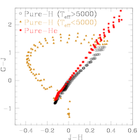
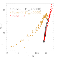
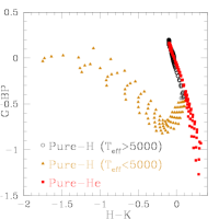
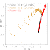
Figure 11: Several colour-colour diagrams obtained using Gaia and 2MASS passbands for all $T_{\mathrm{eff}}$.

5 Classification and parametrisation

The spectrophotometric instrument onboard Gaia has been designed to allow the classification of the observed objects and their posterior parametrisation. The classification and parametrisation will be advantageous in front of other existing or planned photometric surveys because of the combination of spectrophotometric and astrometric Gaia capabilities. The extremely precise parallaxes will permit one to decontaminate the WD population from cool MS stars or subdwarfs. Parallaxes are especially important for very cool WDs ($T_{\mathrm{eff}}$ $<5000$ K) since Gaia will provide the necessary data to derive the masses of already known WDs (for the first time) and newly discovered cool WDs.

The classification and a basic parametrisation of the sources will be provided in the intermediate and final Gaia data releases in addition to the spectrophotometry and integrated photometry. This classification and parametrisation process will be performed by the Gaia Data Processing and Analysis Consortium, which is in charge of the whole data processing, and will be based on all astrometric, spectrophotometric, and spectroscopic Gaia data (Bailer-Jones et al. 2013). The purpose here is not to define or describe the methods to be used to determine the astrophysical parameters of WDs, but just to provide some clues on how to obtain from Gaia the relevant information to derive the temperature, surface gravity, and composition of WDs.

Effective temperature:

in Fig. 12, we can see the strong correlation between $G_{\rm BP}$ $-$ $G_{\rm RP}$ colour and $T_{\mathrm{eff}}$ valid for all compositions when $T_{\mathrm{eff}}$ $>5000$ K, while for the cool regime the colour-temperature relationship depends on the composition and the surface gravity. The flux depression in the IR due to CIA opacities in pure-H and mixed compositions causes that the relationship presents a turnaround at $G_{\rm BP}$ $-$ $G_{\rm RP}$ $\sim 1.7$. WDs with $G_{\rm BP}$ $-$ $G_{\rm RP}$ $>1.7$ most likely have pure-He composition and $T_{\mathrm{eff}}$ $\sim 3000$–$4000$ K. Therefore, Gaia is expected to shed light on the atmospheric composition of the coolest WDs.

$G_{\rm BP}$ $-$ $G_{\rm RP}$ colours for the WDs observed by SDSS and included in Kilic et al. (2010a) have been computed from their $g-z$ colours using the polynomial expressions in Table 6 (available online) and are also included in Fig. 12 for comparison purposes. Assuming that a prior classification in the ’normal’ or cool regime has been performed from parallax information, the $G_{\rm BP}$$-$$G_{\rm RP}$ vs $T_{\mathrm{eff}}$ relationship can be used to derive temperatures. The slope of the relationship for pure-He WDs and the expected errors of $G_{\rm BP}$ $-$ $G_{\rm RP}$ (estimated from Gaia expected performances webpage²) were used to compute the $T_{\mathrm{eff}}$ errors for the Kilic et al. (2010a) WDs (Fig. 13). From these SDSS WDs we found a mean $\sigma_{T_{\rm eff}}/T_{\rm eff}$ of $\sim 1$%.

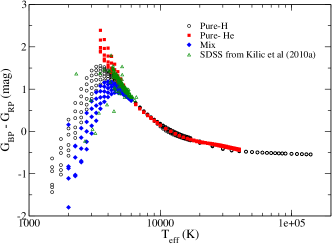
Figure 12: $G_{\rm BP}$-$G_{\rm RP}$ colour dependency with $T_{\mathrm{eff}}$ for pure-H (black), pure-He (red), or mixed composition (blue) WDs. WDs observed by SDSS and included in Kilic et al. (2010a) are also plotted (in green).

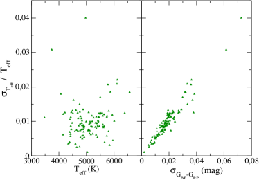
Figure 13: Relative error in $T_{\mathrm{eff}}$ derived for real WDs observed by SDSS and extracted from Kilic et al. (2010a) as a function of $T_{\mathrm{eff}}$ (left) and of the uncertainty in Gaia $G_{\rm BP}$$-$$G_{\rm RP}$ colour (right).

Surface gravity:

the spectral region around $\lambda=360$–$500$ nm with the hydrogen Balmer lines is particularly useful to derive the surface gravity. Although the transmission of $G_{\rm BP}$ is low at this wavelength range, the end-of-mission signal-to-noise ratio is better than 15 for $G\leq 16.5$ (if $T_{\mathrm{eff}}$ $=5000$ K) or even $G\leq 17.7$ (if $T_{\mathrm{eff}}$ $=40\,000$ K). Unfortunately, it is doubtful that precise atmospheric parameters determination can be performed with Gaia BP/RP spectra alone because of the low resolution of the BP/RP instruments. We recall that by combining the Gaia parallaxes and magnitudes with $T_{\mathrm{eff}}$ estimates as described above and a theoretical mass-radius relationship for WDs, it is possible to derive fairly precise $\log g$ values.

Chemical composition:

the difference between pure-H and pure-He is visible in the Balmer jump (with a maximum around $T_{\mathrm{eff}}$ $\sim 13\,000$ K) and the analysis of BP/RP of WD spectra (not only their colours) will help to identify the differences in composition (see Fig. 3). However, to determine atmospheric parameters, it will be better to use Gaia photometry constrained by the parallax information. Additional observations may be necessary to achieve a better accuracy on the atmospheric parameters, such as additional photometry or higher resolution spectroscopic follow-up. A comparison of the masses obtained from the Gaia parallaxes with those determined from spectroscopic follow-up will allow one to test the mass-radius relations and the internal chemical composition for WDs.

The Gaia RVS range around 860 nm is not optimal to see features in WD SEDs (only DZ and similar rare WDs with metal lines will show some features in this region). Ground-based follow-up spectroscopic observations around the hydrogen Balmer lines need to be obtained to derive radial velocities and abundances.

The SED of the pure-H and pure-He WDs differ considerably in the IR wavelength range, particularly in the cool domain (see Fig. 1), and thus, the combination of Gaia and IR photometry will allow one to disctinguish among compositions. Figure 11 shows Gaia$-$2MASS colour-colour diagrams. The all-sky 2MASS catalogue can be used for WDs brighter than $J=16.5$, $H=16.5$ and $K=16$, which are the limiting magnitudes of the survey. Gaia goes much fainter, and therefore near-IR surveys such as the UKIDSS Large Area Survey ($J_{\rm lim}=20$, $K_{\rm lim}=18.4$, Hewett et al. 2006), VIKING (VISTA Kilo-Degree Infrared Galaxy Survey; $J_{\rm lim}=20.9$, Findlay et al. 2012), and VHS (VISTA Hemisphere Survey, $J_{\rm lim}=21.2$, Arnaboldi et al. 2010) will be of great interest, although they only cover $4000$, $1500$, and $20\,000$ deg², respectively.

6 White dwarfs in the Galaxy

The currently known population of WDs amounts to $\sim$ $20\,000$ objects (Kleinman et al. 2013). This census will be tremendously increased with the Gaia all-sky deep survey, and more significantly for the halo population and the cool regime (Torres et al. 2005). We present estimates of the number of WDs that will be observed (see Tables 9 – 10 and Figs. 14 – 17) according to two different simulations: one extracted from the Gaia Universe Model Snapshot (GUMS, Robin et al. 2012) and another one based on Napiwotzki (2009). These simulations (which only include pure-H WDs) were adapted to provide Gaia -observed samples (limited to $G=20$). Both simulations build their stellar content based on the galactic structure in the Besançon Galaxy Model, (BGM, Robin et al. 2003), but some differences were considered in each simulation since then.

The BGM considers four different stellar populations: thin disc, thick disc, halo, and bulge, of which the latter has little relevance for our simulations and will thus not be discussed any further. An age-dependent scale height is adopted for the thin disc and both WD simulations assume a constant formation rate of thin-disc stars. The thick disc is modelled with a scale height of 800 pc, and the stellar halo as a flattened spheroid.

Although the ingredients of the simulations have been detailed in the original papers, we briefly summarize in Sects. 6.1 and 6.2 some relevant information for each simulation to help understand their compared results in Sect. 6.3.

6.1 Simulations using GUMS

GUMS provides the theoretical Universe Model Snapshot seen by Gaia and is being used for mission preparation and commissioning phases. It can be used to generate stellar catalogues for any given direction and returns information on each star, such as magnitude, colour, and distance, as well as kinematics and other stellar parameters. Although only WD simulations were extracted, GUMS also includes many Galactic and extra-galactic objects, and within the Galaxy it includes isolated, double, and multiple stars as well as variability and exoplanets. The ingredients of GUMS regarding the WD population are summarized here:

• Thin-disc WDs are modelled following the Fontaine et al. (2001) pure-H WD evolutionary tracks, assuming the Wood (1992) LF for an age of 10 Gyr and an IMF from Salpeter (1955). It has been normalised to provide the same number of WDs of $M_{V}\leq 13$ as derived by Liebert et al. (2005) from the Palomar Green Survey. The photometry was calculated by Bergeron et al. (2011).

• For the thick disc, the WD models of Chabrier (1999) were used assuming an age of 12 Gyr. For the normalisation, the ratio between the number of MS turn-off stars and the number of WDs depends on the IMF and on the initial-to-final mass relation, assuming that all stars with a mass greater than the mass at the turn-off ($M_{TO}=0.83$ M_⊙) are now WDs. However, the predicted number of thick-disc WDs with this assumption is much higher than the number of observed WDs in the Oppenheimer et al. (2001) photographic survey of WDs. This led Reylé et al. (2001) to normalise the thick-disc WD LF to that of the Oppenheimer et al. (2001) sample, assuming it is complete: the ratio between the number of WDs (initial mass $>0.83$ M_⊙) and the number of MS stars (initial mass $<0.83$ M_⊙) is taken to be 20%.

  Because the completeness of the Oppenheimer et al. (2001) sample is not certain, this value can be considered as a lower limit. This normalisation also agrees with the number of WDs in the expanded Luyten half-second proper motion catalogue (LHS) WD sample (Liebert et al. 1999).

• The halo LF is derived from the truncated power-law initial mass function IMF2 of Chabrier (1999) with an age of 14 Gyr. It was specifically defined to generate a significant number of MACHOS in the halo to explain the number of microlensing events towards the Magellanic Clouds. Hence the density of halo WDs is assumed to be 2% of the density of the dark halo locally. Because of the assumed IMF, which is highest at M $=2.4$ M_⊙, the generated WDs have cooled down with an LF peaking at $M_{V}\approx 16.5-17$. Hence the number of halo WDs observable at $G<20$ is rather small (see Table 9), despite their large local density. This is one of the main differences (see Sect. 6.3) with respect to simulations obtained with Napiwotzki (2009). The total local density for each population is included in Table 8.

• GUMS adopts the 3D extinction model by Drimmel et al. (2003).

Table 8: Local densities used in both WD Galaxy simulations, expressed in M${}_{\odot}\cdot$ pc^-3.

	Napiwotzki (2009)	GUMS
Thin	$2.9\cdot 10^{-3}$	$4.16\cdot 10^{-3}$
Thick	$1.7\cdot 10^{-3}$	$5.06\cdot 10^{-4}$
Halo	$2.7\cdot 10^{-4}$	$2.80\cdot 10^{-4}$

6.1.1 Variable and binary WDs

• Several types of intrinsic stellar variability were considered, and for WDs, they include pulsation of ZZ-Ceti type, cataclysmic dwarfs, and classical novae types. For WDs in close-binary systems (period shorter than 14 hours), half of them are simulated as dwarf novae and the other half as classical novae. WD$+$WD close-binary systems are also considered in these simulations.

• Although the simulation of binaries is already quite realistic in GUMS, it still needs some further refinement in the specific case of WDs.

  Work is on-going to improve the mass distribution in new versions of the Gaia simulator. For this reason, we are still unable to detail the number of WDs in binary systems in which orbital parameters can be obtained to provide independent mass estimates of the WDs. This study will be possible with future versions of the GUMS simulations.

6.2 Simulations using Napiwotzki (2009)

Napiwotzki (2009) used the Galactic model structure of BGM to randomly assign positions of a large number of stars based on observed densities of the local WD population. Depending on population membership, each star is given a metallicity, an initial mass, and kinematical properties. The ingredients are summarized in the following items:

• The WD cooling sequences were created by combining the tracks of Blöcker (1995) for hot WDs with the sequences of Fontaine et al. (2001) for cooler WDs.

• The WD progenitor lifetime was calculated from the stellar tracks of Girardi et al. (2000).

• The initial-final mass relationship by Weidemann (2000) was considered.

• The relative contributions of each Galactic population were calibrated using the kinematic study of Pauli et al. (2006) of the brightness-limited SPY (ESO SN Ia Progenitor Survey: Napiwotzki et al. 2001) sample. Pauli et al. (2006) assigned population membership according to a set of criteria based on the measured 3D space velocity. An iterative correction for mis-assignment of membership of WDs with ambiguous kinematic properties was derived from the model (see Napiwotzki 2009).

• Space densities were then calculated from the relative contributions and the WD numbers in the 13 pc sample of Holberg et al. (2008). The finally adopted local densities can be seen in Table 8.

• Holberg & Bergeron (2006) colour tables were used for WD simulations, and photometric transformation from Table 6 of the present paper were used to carry out the brightness selection for the Gaia sample.

• IMFs from Salpeter (1955) were used to derive numbers in Table 9, although other IMFs (e.g. Chabrier 1999; Baugh et al. 2005) were tested as well. These would give higher numbers of cool, high mass WDs.

Napiwotzki (2009) compared the simulations with the proper-motion-selected sample of Oppenheimer et al. (2001). Simulated numbers turned out to be slightly higher, which can easily be explained by a minor incompleteness of the observed sample.

6.3 Results

Table 9 shows the number of WDs detectable for each population (about $200\,000$–$250\,000$ single WDs in total) according to the two simulations explained above. Table 10 shows the expected number and types of variable WDs observed by Gaia, according to GUMS.

Table 9: Total number of WDs with $G\leq 20$ expected in Gaia for different $T_{\mathrm{eff}}$ ranges.

$T_{\mathrm{eff}}$	$N_{\rm Thin}$	$N_{\rm Thick}$	$N_{\rm Halo}$
Napiwotzki (2009)
All range, single	$196\,765$	$48\,673$	$9705$
$<5000$ K, single	$925$	$1883$	$347$
GUMS
All range, single	$198\,107$	$3557$	63
All range, Comp A	$64\,905$	$2340$	47
All range, Comp B	$296\,976$	$1153$	4
$<5000$ K, single	$8845$	142	63
$<5000$ K, Comp A	862	95	47
$<5000$ K, Comp B	244	12	4

Table 10: Number and types of variable WDs as predicted by GUMS.

Variables	ZZCeti	Dwarf	Classical
		Novae	Novae
Isolated	$18\,363$	–	–
In binary	$6463$	340	$10\,258$

Most of the observed WDs belong to the thin disc because of the still on-going star formation. The number of thin-disc WDs in the two simulations agree remarkably well at the level of 1% for single stars. We note that in GUMS binaries are added and produce about $3.6\cdot 10^{5}$ additional thin-disc WDs (see Table 9). However, this estimate includes WDs in binary systems that are not resolvable by Gaia alone. Just for comparison, previous estimates of the number of WDs in the disc reported by Torres et al. (2005) provided $3.9\cdot 10^{5}$ WDs with $G<20$ mag.

The small number of WDs known in thick-disc and halo populations is the current limiting factor to constrain their properties. Due to these limitation, Napiwotzki (2009) and GUMS arrive at different interpretations of the Oppenheimer et al. (2001) sample. The local thick-disc density assumed by Napiwotzki (2009) is three times higher than the one assumed by GUMS (see Table 8). The local densities for the halo are more similar, but the more stringent difference comes from the shapes of the assumed LF and the IMFs. The IMF assumed by GUMS leads to a very low estimated number of thick-disc and halo WDs observable by Gaia.

As expected, the number of observable cool WDs ($T_{\mathrm{eff}}$ $<5000$ K) of all populations will be considerably smaller than the total sample. However, this will still represent a dramatic increase compared with any previous survey (e.g. only 35 cool WDs were found in the SDSS sample by Harris et al. 2006).

In addition to this increase in the number of cool WDs, one of the main contributions of the Gaia mission will also be the large portion of sources with good parallaxes (see Table 2 for estimates of the number of WDs observed in all temperature regimes). For cool WDs ($T_{\mathrm{eff}}$ $<5000$ K), GUMS estimates about $2000$ with $\frac{\sigma_{\pi}}{\pi}<1\%$ ($20\%$ of all predicted cool WDs). Furthermore, the complete sample of about 9000 observed cool WDs will have $\frac{\sigma_{\pi}}{\pi}<5.5\%$. Table 2 shows that all cool ($T_{\mathrm{eff}}$ $<7000$ K) WDs in the Kilic et al. (2010a) sample extracted from SDSS will have $\frac{\sigma_{\pi}}{\pi}<5\%$ when observed with Gaia.

The resulting WDs $M_{V}$ distributions are plotted in Figs. 14 and 15 for Napiwotzki (2009) and GUMS simulations, respectively. Values higher than average $M_{V}$ are more frequent for thick-disc and halo populations than for thin-disc populations, especially in the Napiwotzki (2009) simulations. These represent the oldest WDs ($>10$ Gyr) produced from higher mass progenitors (with much higher masses than the $0.45$–$0.50$ M_⊙ WDs that dominate brightness-limited samples of halo WDs). IMFs such as those from Chabrier (1999); Baugh et al. (2005) would enhance these tails resulting in much higher numbers of cool WDs.

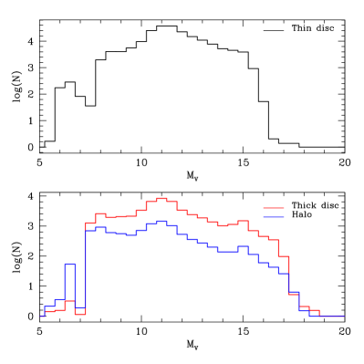
Figure 14: Simulated Gaia $M_{V}$ distribution of a single WD population with $G<20$ mag from thin-disc (top panel), thick-disc and halo populations (bottom panel) based on Napiwotzki (2009).

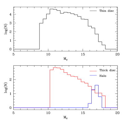
Figure 15: Same as Fig. 14, now using GUMS simulations.

Differences in the number of predicted WDs can also be seen in the $T_{\mathrm{eff}}$ and $\log g$ histograms plotted in Fig. 16. In GUMS there are no halo WDs hotter than about 5000 K because of the type of IMF is assumed with an age of 14 Gyr. Thus, the detection and identification of these old massive WDs with Gaia will be extremely helpful to obtain information about the IMF of the Galaxy. The peak of the $T_{\mathrm{eff}}$ distribution for Napiwotzki (2009) shown in Fig. 16 (top) is centred around $12\,000$ K, which is the result of the interplay between the WD cooling rate and the change of absolute brightness with temperature.

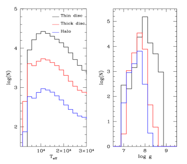
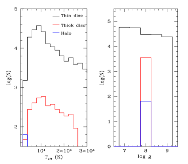
Figure 16: Comparison of $T_{\mathrm{eff}}$ and $\log g$ histograms for single WDs in thin-disc, thick-disc, and halo populations obtained using Napiwotzki 2009 (upper panels) and GUMS simulations (bottom panels). GUMS halo and thick-disc WDs are assumed to have $\log g=8.0$.

The present version of GUMS considers only discrete values for $\log g$ (from $7.0$ to $9.0$ in steps of $0.5$). In particular, for the thick-disc and halo WDs only $\log g=8.0$ was assumed (see Fig. 16). In the simulations of Napiwotzki (2009), the peak tends to be lower for the thick-disc and halo populations than for the thin disc. This agrees with the results obtained by the SPY project (Pauli et al. 2006), showing that hot WDs ($T_{\mathrm{eff}}$ $>10\,000$ K) that belongs to the halo population have masses in the range $0.45$–$0.50$ M_⊙.

The predicted HR diagram in Gaia observables is shown in Fig. 17. According to Fig. 18 in Robin et al. (2012), the low-mass MS can be perfectly separated from the WD branch (at least for $T_{\mathrm{eff}}$ $>3000$ K). Therefore, we will be able to separate cool WDs from cool MS stars in the Gaia catalogues.

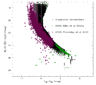
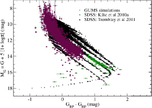
Figure 17: Hertzsprung–Russell diagram built using only Gaia observable quantities ($G$, $G_{BP}$, $G_{RP}$, and parallaxes) for single WDs with $G\leq 20$ obtained from Napiwotzki (2009), top, and GUMS, bottom. The Hertzsprung–Russell GUMS diagram considers discrete values for $\log g$, which is reflected as quantised trends in this plot. SDSS WD samples extracted from Tremblay et al. (2011) and Kilic et al. (2010a) are overplotted with error bars as expected from Gaia observations. Table 2 shows that almost all SDSS WD plotted here have relative error of parallaxes better than 10%.

We did not aim to discuss which of the two simulations considered here better reproduces the reality, but only to provide an estimate of the number of WDs in different stellar populations predicted to be observed by Gaia. On the other hand, a comparison of the true Gaia data with our simulations will improve our knowledge about the Milky Way formation and validate the models and assumptions.

7 Summary and conclusions

We have presented colour-colour photometric transformations between Gaia and other common optical and IR photometric systems (Johnson-Cousins, SDSS and 2MASS) for the case of WDs. To compute these transformations the most recent Gaia passbands and WD SED synthetic libraries (Tremblay et al. 2011; Bergeron et al. 2011) were used.

Two different behaviours were observed depending on the WD effective temperature. In the ’normal’ regime ($T_{\mathrm{eff}}$ $>5000$ K) all WDs with the same composition (pure-H or pure-He) could be fitted by a single law to transform colours into the Gaia photometric system. For the very cool regime, WDs with different compositions, $T_{\mathrm{eff}}$ and $\log g$, fall in different positions in colour-colour diagram which produces a spread in these diagrams. Colours with blue/UV information, like the $B$ Johnson passband, seem to better disctinguish the different WD characteristics, but the measurements in this regime will be rather noisy because of the low photon counts for very cool sources and in practice might be hard to use. We therefore expect that observations in near-IR passbands, combined with Gaia data, might be very helpful in characterising WDs, especially in the cool regime.

Estimates of the number of WDs that Gaia is expected to observe during its five-year mission and the expected precision in parallax were also provided. According to the number of sources predicted by Napiwotzki (2009) and by the Gaia Universe Model Snapshot (Robin et al. 2012), we expect between $250\,000$ and $500\,000$ WDs detected by Gaia. A few thousand of them will have $T_{\mathrm{eff}}$ $<5000$ K, which will increase the statistics of these very cool WDs quite substantially, a regime in which only very few objects have been observed until now (Catalán et al. 2012; Harris et al. 2006).

Gaia parallaxes will be extremely important for the identification and characterisation of WDs. We provided estimates of the precision in WD parallaxes that Gaia will derive, obtaining that about $95\%$ of WDs will have parallaxes better than $10\%$. For cool WDs ($T_{\mathrm{eff}}$$<5000$ K) they will have parallaxes better than $5\%$, and about $2000$ of them will have parallaxes better than $1\%$.

Additional photometry or/and spectroscopic follow-up might be necessary to achieve a better accuracy on the atmospheric parameters. A comparison of the masses obtained from the Gaia parallaxes with those determined from spectroscopic fits will allow testing the mass-radius relations for WDs. A better characterisation of the coolest WDs will also be possible since it will help to resolve the discrepancy regarding the H/He atmospheric composition of these WDs that exist in the literature (Kowalski & Saumon 2006; Kilic et al. 2009b, 2010a). In addition,, the orbital solutions derived for the WDs detected in binary systems will provide independent mass determinations for them, and therefore will allow for stringent tests of the atmosphere models. This will improve the stellar population ages derived by means of the WD cosmochronology and our understanding of the stellar evolution.