Adaptive MCMC-Based Inference in Probabilistic Logic Programs

Abstract

Probabilistic Logic Programming (PLP) languages enable programmers to specify systems that combine logical models with statistical knowledge. The inference problem, to determine the probability of query answers in PLP, is intractable in general, thereby motivating the need for approximate techniques. In this paper, we present a technique for approximate inference of conditional probabilities for PLP queries. It is an Adaptive Markov Chain Monte Carlo (MCMC) technique, where the distribution from which samples are drawn is modified as the Markov Chain is explored. In particular, the distribution is progressively modified to increase the likelihood that a generated sample is consistent with evidence. In our context, each sample is uniquely characterized by the outcomes of a set of random variables. Inspired by reinforcement learning, our technique propagates rewards to random variable/outcome pairs used in a sample based on whether the sample was consistent or not. The cumulative rewards of each outcome is used to derive a new “adapted distribution” for each random variable. For a sequence of samples, the distributions are progressively adapted after each sample. For a query with “Markovian evaluation structure”, we show that the adapted distribution of samples converges to the query’s conditional probability distribution. For Markovian queries, we present a modified adaptation process that can be used in adaptive MCMC as well as adaptive independent sampling. We empirically evaluate the effectiveness of the adaptive sampling methods for queries with and without Markovian evaluation structure.

1 Introduction

Probabilistic Logic Programming (PLP) covers a class of Statistical Relational Learning frameworks Getoor and Taskar (2007) aimed at combining logical and statistical reasoning. Examples of languages and systems combining logical and statistical inference include ICL Poole (1997), SLP Muggleton et al. (1996), PRISM Sato and Kameya (1997), LPAD Vennekens and Verbaeten (2003) and ProbLog De Raedt et al. (2007). In addition to standard statistical models, these languages allow reasoning over many models where logical and statistical knowledge is intricately combined, and cannot be expressed as standard statistical models.

An example problem with such a model is reachability over finite probabilistic graphs, i.e., graphs in which the presence or absence of edges is determined by a set of independent probabilistic processes. Fig. 1(a) shows an example of a probabilistic graph, where labels on the edges denote the probability with which that edge is present. For instance, edge $(a,b)$ is present with probability $0.9$ while edge $(b,e)$ is present with probability $0.01$. The logical relationship between reachability of $e$ from $a$, and the underlying edges in the graph cannot be expressed concisely in standard probabilistic frameworks. A PRISM program encoding this problem is shown in Fig. 1(b).

As illustrated in Fig. 1(b), PRISM adds probabilistic facts of the form $\mbox{\tt msw}(s,i,t)$ where $s$ is a term representing a random process called a switch, $i$ an instance of the switch, and $t$ its outcome. The range of a switch is specified by “value” declarations; and its distribution is specified by “set_sw” declarations. A possible world associates an outcome with each switch instance, and can be seen as a set of msw facts external to the program. In each possible world, the PRISM program, together with msw facts defining the world is a non-probabilistic program; the distribution over the possible worlds induces a distribution over the models of the PRISM program. Such a declarative distribution semantics originally defined for ICL and PRISM has been defined for other PLP languages such as LPAD and ProbLog as well.

⬇ 1% Possible edges 2poss_edge(a,b). 3poss_edge(a,c). 4poss_edge(b,d). 5poss_edge(b,e). 6poss_edge(c,d). 7poss_edge(c,e). ⬇ 1% Random processes 2values(r(_,_), [t,f]). 3% Distributions 4:- set_sw(r(a,b), [0.9,0.1]). 5:- set_sw(r(a,c), [0.2,0.8]). 6:- set_sw(r(b,d), [0.8,0.2]). 7:- set_sw(r(b,e), [0.01,0.99]). 8:- set_sw(r(c,d), [0.7,0.3]). 9:- set_sw(r(c,e), [0.1,0.9]). ⬇ 7% Edge: 8edge(X,Y) :- 9 poss_edge(X,Y), 10 msw(r(X,Y),t). 11% Reachability on acyclic graphs 12reach(X,Y) :- edge(X,Y). 13reach(X,Y) :- 14 edge(X,Z), 15 reach(Z,Y).

(a)

(b)

Figure 1: Example: (a) Probabilistic Graph; (b) Reachability over probabilistic graphs in PRISM

Motivation.

While PLPs can concisely express such problems, typical implementations of PLP systems have limitations. For instance, PRISM’s standard inference technique is based on enumerating explanations for answers, treating the set of explanations as pairwise mutually exclusive; in fact, due to this limitation the probability of reach(a,e) in the above example cannot be computed in PRISM. ProbLog, and subsequently, PITA Riguzzi and Swift (2011), removed these restrictions; however, exact inference in these systems does not scale beyond graphs with a few hundred vertices.

Of the several powerful sampling-based techniques developed for statistical reasoning, Markov Chain Monte Carlo (MCMC) techniques are especially suited for inference in PLPs, as shown by Cussens (2000) and Moldovan et al. (2013).

The Problem.

PLP queries for evaluating conditional probabilities are called as conditional queries and denoted as $\mathtt{prob}(q\mid e)$, where $q$ and $e$ are ground atomic goals, called query and evidence, respectively. A conditional query $\mathtt{prob}(q\mid e)$ denotes a suitably normalized distribution of $q$ over all possible worlds where $e$ holds. Existing PLP systems either provide efficient techniques that apply to a restricted class of $q$ and $e$ (e.g., hindsight in PRISM) or do not treat evidence specially, leading to poor performance especially when the likelihood of evidence is low. For instance, consider the problem of determining the probability that $d$ is reachable from $a$, given that $e$ is reachable from $a$ (i.e. $\mathtt{prob}(\mathtt{reach(a,d)}\mid\mathtt{reach(a,e)})$, over the probabilistic graph in Fig. 1(a). Techniques such as the one proposed by Moldovan et al. (2013) will generate a world and reject it if evidence does not hold in the world. Since the probability that $e$ is reachable is $0.02882$, a large percentage of generated worlds will be inconsistent with the evidence, and hence unusable for computing the conditional probability.

The problem of efficiently estimating the conditional probability, even when the likelihood of evidence is low, has remained unaddressed in the context of PLP. We explore this problem in this paper, by developing an Adaptive Markov Chain Monte Carlo (AMCMC) technique. Following adaptive MCMC techniques in statistical reasoning, we progressively modify the distribution from which samples are derived; we modify the distribution so as to favor those samples that are consistent with evidence. The adaptive sampler reduces the number of generated samples needed to estimate the conditional probability to a given precision.

Approach Overview.

Our technical development starts with a MCMC technique where each state of the Markov Chain is an assignment of values to a set of switch instances. An assignment at a state corresponds to a set of possible worlds such that the truth values of evidence and query are identical in all the worlds in the set. Transitions are proposed on this chain by resampling one or more switch instances in the state and extending the resulting assignment to another state. A Metropolis-Hastings Hastings (1970) sampler is used to accept or reject this proposal, yielding the next state in the chain.

To this basic MCMC technique, we introduce adaptation as follows. For each switch instance/outcome pair, we maintain Q-value which is the likelihood that an evaluation of the evidence goal using that switch instance/outcome will succeed. Q-values are computed by maintaining a sequence of switch instances and outcomes used to evaluate the evidence goal, and propagating rewards through this sequence depending on the success or failure of the evaluation. The adapted distribution of a switch instance is proportional to the original distribution weighted by (normalized) Q-values of each outcome.

Although motivated by problems where the likelihood of evidence is low, the technique we describe is more generally applicable, even to unconditional queries.

Summary of Contributions.

1. We define a MCMC procedure where states of the Markov chain are sets of possible worlds. This procedure is largely independent of LP evaluation itself, and hence can be used for approximate inference in probabilistic logic programs extended with tabling, constraint handling, or other features (Section 3).

2. We define an adaptation procedure to modify the distribution from which samples are drawn. The aim of the adaption is to increase the likelihood that a sample will be consistent with given evidence (if any). We show that the adaption satisfies the “diminishing adaption” condition and hence can be used to effectively to adapt an MCMC procedure (Section 4).

3. For a class of queries satisfying a “Markovian evaluation structure”, the adapted distribution of a random variable coincides with its marginal. For such queries, we obtain an alternative adaption procedure that can be used to obtain an adaptive independent sampler (Section 4).

We describe the results of our preliminary experiments to evaluate the MCMC procedure as well as the adaptation procedure in Section 5.

The rest of the paper begins with a brief overview of MCMC in Section 2. A more detailed description of related work and concluding remarks appears Section 6.

2 Preliminaries: Markov Chain Monte Carlo Techniques

A sequence of random variables $X^{(i)},i\geq 0$ taking on values $x^{(i)}$ is called a Markov chain if $P(x^{(i)}|x^{(i-1)},x^{(i-2)},$ $\ldots,x^{(1)})=P(x^{(i)}|x^{(i-1)})$ Andrieu et al. (2003). The values of the random variables are chosen from a fixed set called the state space of the Markov chain. When the state space is finite, the one step transition probabilities between various states are generally given as a matrix known as the transition kernel.

Given a distribution on the values of $X^{(0)}$, the distribution on the values of any $X^{(i)},i>0$ can be computed by multiplying the transition kernel $i$ times with the initial distribution. For certain Markov chains, irrespective of the initial distribution on $X^{(0)}$, the distribution on the of values $X^{(n)}$ converges as $n$ increases, to its limiting distribution or stationary distribution. More formally, a stationary distribution $\pi$ with respect to a Markov chain with transition kernel $A$ satisfies the condition $\pi=\pi A$. Irreducible and aperiodic Markov chains have a unique stationary distribution Andrieu et al. (2003). In practice, a distribution $\pi$ is verified to be a stationary distribution, if for any two states $x$ and $y$ the following detailed balance condition holds.

$$\pi(x)A(x,y)=\pi(y)A(y,x)$$

Given a hard to sample target distribution, MCMC techniques solve the problem by constructing a Markov chain whose stationary distribution is the target distribution and drawing samples from it. Metropolis-Hastings (MH) is a popular MCMC-based sampling technique. Given a target distribution $\pi$ and an irreducible, aperiodic Markov chain with transition kernel $A$, the MH sampler proposes a transition from state $x$ to $y$ according to $A(x,y)$, but then accepts or rejects this proposal according to the acceptance probability $min\{1,\frac{\pi(y)A(y,x)}{\pi(x)A(x,y)}\}$ Hastings (1970).

Adaptive MCMC

Given a target distribution from which samples need to be generated, MCMC algorithms such as MH construct a Markov chain whose transition kernel satisfies the detailed balance condition with respect to the target distribution. However, there are several transition kernels which satisfy this requirement. The optimal choice is not always clear. In such situations adaptive MCMC algorithms tune the transition kernel as the chain proceeds Roberts and Rosenthal (2007).

The total variation distance between two distributions $P$ and $Q$ is defined as $\|P-Q\|=\frac{1}{2}\sum_{x}|P(x)-Q(x)|$ Levin et al. (2009). A Markov chain with transition kernel $A$ is said to be ergodic with respect to a target distribution $\pi$ if $lim_{n\rightarrow\infty}\|A^{n}(x,.)-\pi(.)\|=0$, for all $x$ Roberts and Rosenthal (2007). In other words, the rows of the transition matrix converge to the target distribution as it is repeatedly multiplied with itself. It also means that irrespective of which state we start in the long term probability of being in a state converges to the probability of that state given by the target distribution. In general, adaptation of a transition kernel does not preserve ergodicity of the Markov chain with respect to the target distribution. However, ergodicity has been shown to be preserved under certain conditions, namely performing adaptation at regeneration times Gilks et al. (1998); Brockwell and Kadane (2005) and diminishing adaptation Roberts and Rosenthal (2007, 2009). We use the latter condition for preserving ergodicity in our adaptation scheme.

Ergodicity conditions.

Given a family of transition kernels $\{P_{\Gamma_{1}},P_{\Gamma_{2}},\ldots\}$, each having the target distribution $\pi$ as the stationary distribution, adaptive MCMC algorithms choose the transition kernel $P_{\Gamma_{i}}$ at time step $i$. The update rule of $P_{\Gamma_{i}}$ is specified by the adaptive algorithm. Then ergodicity is preserved if all transition kernels have simultaneous uniform ergodicity, namely,

$$\text{For each }\varepsilon>0,\text{ there exists }N=N(\varepsilon)\in\mathbb{N}\text{ such that }\|P_{\gamma}^{N}(x,.)-\pi(.)\|\leq\varepsilon\text{ for all }x\text{ and }\gamma$$

and the following diminishing adaptation condition is satisfied. Roberts and Rosenthal (2007).

$$\lim_{n\to\infty}\text{sup}\|P_{\Gamma_{n+1}}(x,.)-P_{\Gamma_{n}}(x,.)\|=0\text{ in probability}$$

3 MCMC for Probabilistic Logic Programs

The ability to treat a PRISM program as non-probabilistic in each world also helps us in designing sample-based query evaluation. Given a PRISM program $P$ and a ground goal $q$, we lazily construct a set of worlds by sampling, such that $q$ succeeds or fails in all worlds in the set. The set of worlds are represented by assignments described below.

3.1 Sample-Based Query Evaluation

Assignments.

We use a structure called an assignment to keep track of known outcomes of switch instances when sampling from a PRISM program. An assignment is denoted by partial function $\sigma$ such that $\sigma(s,i)$ is the value of instance $i$ of switch $s$. Note that $\sigma$ represents a set of worlds; the set of worlds corresponding to $\sigma$ is denoted by $\mbox{\it worlds\/}(\sigma)$.

Let $\sigma$ be an assignment. We say $\sigma^{\prime}=\sigma[(s,i)\rightarrow v]$ is an assignment that is identical to $\sigma$ at every point except at $(s,i)$ where $\sigma^{\prime}(s,i)=v$. We define a partial order “$\succeq$” over assignments: $\sigma^{\prime}\succeq\sigma$ if $\sigma^{\prime}(s,i)=\sigma(s,i)$ whenever $\sigma(s,i)\not=\bot$. We also say that $\sigma^{\prime}$ extends $\sigma$ if $\sigma^{\prime}\succeq\sigma$. We say that two assignments $\sigma$ and $\sigma^{\prime}$ are mutually exclusive, denoted by $\sigma\parallel\sigma^{\prime}$, if there is some switch instance $(s,i)$ such that both $\sigma$ and $\sigma^{\prime}$ are defined at $(s,i)$, but $\sigma(s,i)\not=\sigma^{\prime}(s,i)$. Two assignments are compatible (denoted by “$\nparallel$”) if they are not mutually exclusive.

Given a switch $s$, we denote by $\mbox{\it random\/}(s)$ a value randomly drawn from the domain of $s$ using the probability distribution defined for $s$. For looking up in an assignment or extending an assignment, we define a function pick_value, defined as follows:

$$\begin{array}[]{rcl}\mbox{\it pick\_value\/}(\sigma,s,i)&=&\left\{\begin{array}[]{ll}\langle v,\sigma\rangle&\mbox{if $\sigma(s,i)=v\not=\bot$ }\\ \langle v,\sigma[(s,i)\mapsto v]\rangle&\mbox{if $\sigma(s,i)=\bot$ and $v=\mbox{\it random\/}(s)$}\\ \end{array}\right.\end{array}$$

Note that pick_value is non-decreasing in the sense that if $\langle v,\sigma^{\prime}\rangle=\mbox{\it pick\_value\/}(\sigma,s,i)$, then $\sigma^{\prime}\succeq\sigma$. Alternatively, we can view $\mbox{\it pick\_value\/}(\sigma,s,i)$ as defining a distribution, generating $\langle v,\sigma\rangle$ with probability $1$ if $\sigma(s,i)=v$; and $\langle v,\sigma^{\prime}\rangle$ where $\sigma^{\prime}=\sigma[(s,i)\mapsto v]$ with probability $P_{s}(v)$ if $\sigma(s,i)=\bot$.

Sampling Evaluators.

We describe the MCMC algorithm parameterized with respect to a probabilistic query evaluation procedure called a Sampling Evaluator. This permits us to describe a generic MCMC algorithm that can be instantiated to extended probabilistic logic programming systems, including tabled and/or constraint probabilistic LPs.

A sampling evaluator, given an assignment $\sigma$ and ground goal $q$, (probabilistically) generates an answer to $q$ (success/failure), denoted by $\mbox{\it ans\/}(q)$, an assignment $\sigma^{\prime}$, and a sequence $\rho$ of switch/instance/outcome triples $(s_{1},i_{1},v_{1}),(s_{2},i_{2},v_{2}),\ldots,(s_{k},i_{k},v_{k})$, $k\geq 0$ such that the following conditions hold:

SE1.

Consider the sequence of assignments $\sigma_{0},\sigma_{1},\ldots,\sigma_{k}$ such that $\sigma_{0}=\emptyset$, and $\sigma_{j+1}=\sigma_{j}[(s_{j+1},i_{j+1})\mapsto v_{j+1}]$ for $0\leq j<k$. Then, $\sigma_{k}=\sigma^{\prime}$. Moreover, $\sigma^{\prime}$ is compatible with $\sigma$, i.e. $\sigma^{\prime}\nparallel\sigma$.

SE2.

If $\mbox{\it ans\/}(q)=\mbox{\it success\/}$ (similarly, failure), then $q$ is true (or false, resp.) in all worlds $w\in\mbox{\it worlds\/}(\sigma^{\prime})$.

Moreover, let $\Sigma$ denote the set of all $\sigma^{\prime}$ generated by the sampling evaluator. Then,

SE3.

If $w$ is a world s.t. $q$ is true (similarly, false) in $w$, then $\exists\sigma^{\prime}\in\Sigma$ such that $w\in\mbox{\it worlds\/}(\sigma^{\prime})$ and $\mbox{\it ans\/}(q)=\mbox{\it success\/}$ (or failure, respectively).

SE4.

Every distinct $\sigma_{a},\sigma_{b}\in\Sigma$ are mutually exclusive: i.e. either $\sigma_{a}=\sigma_{b}$, or $\sigma_{a}\parallel\sigma_{b}$.

Properties SE2 and SE3 correspond to soundness and completeness, respectively. Property SE4 ensures that a sampling evaluator can be used to refine states in an MCMC algorithm. Not all evaluators in a probabilistic logic programming system may satisfy SE4. For instance, if an evaluator is based on constructing explanations for a goal (e.g. as in Problog) since two distinct explanations may not be mutually exclusive, it will violate SE4. Moldovan et al. (2013) overcome this problem by using the Karp-Luby algorithm, resampling switch instances to eliminate overlaps in states. In contrast, we show below that we can use Prolog-style evaluation, performed until the first derivation is found (if one exists) to construct a sampling evaluator i.e. one satisfying the above requirements including SE4.

A sampling evaluator for non-tabled PRISM.

Figure 2 shows the sampling evaluator for non-tabled PRISM programs, constructed by extending the well-known Prolog meta-interpreter. The assignment and the switch/instance/outcome sequence are maintained in the dynamic database. Observe that the evaluation follows that of Prolog as long as the selected literal is not an msw. When the selected literal is of the form $\mbox{\tt msw}(s,i,t)$, we get the value of $(s,i)$ using pick_value, and record this selection. When evaluation produces the empty clause, we know that $q$ has a derivation in all worlds consistent $\sigma$. When every proof finitely fails, we know that $q$ has no derivation in any world that is consistent with $\sigma$. Thus the evaluator in Fig. 2 has the properties described for a sampling evaluator. To see how the procedure satisfies condition SE4, assume to the contrary that the procedure has two executions that generate two assignments, $\sigma_{a}$ and $\sigma_{b}$. Note that the procedure is deterministic and takes the same sequence of steps, except when an msw is encountered. If the two executions picked different outcomes, then $\sigma_{a}\parallel\sigma_{b}$. Otherwise, we can show by induction on the sizes of $\sigma_{a}$ and $\sigma_{b}$, that the assignments are either identical or mutually exclusive.

⬇ 1% Given assignment is in sigma/3; 2% computed assignment is in sigma_prime/3. 3% rho/3 is sequence of switch/instance/outcomes. 4% sigma_prime/3 and rho/3 are initially empty 5:- dynamic sigma/3, sigma_prime/3, rho/3. 6 7% Sampling Evaluator for a ground goal G: 8sample_eval(G) :- eval(G), !. 9 10eval(true) :- !. 11eval((G1,G2)) :- !, eval(G1), eval(G2). 12eval((G1;G2)) :- !, eval(G1); eval(G2). 13eval(msw(S,I,V)) :- !, pick_value(S,I,V). 14eval(G) :- clause(G, B), eval(B). ⬇ 15% Pick value from sigma, 16% extending it via sampling if necessary. 17pick_value(S,I,V) :- 18 (sigma_prime(S,I,U) % if already is defined 19 -> true 20 ; (sigma(S,I,U) % if in current assignment 21 -> assert(sigma_prime(S,I,U)), 22 % genrandom generates a random value U 23 % according to the distribution of S 24 ; genrandom(S,U), 25 assert(sigma_prime(S,I,U)) 26 ), assertz(rho(S,I,U)), % update sequence 27 V=U. % ensure sigma_prime and rho are 28 % updated regardless of given V

Figure 2: Sampling evaluator derived from Prolog meta-interpreter

3.2 MCMC-Based Inference of Conditional Probabilities

Initial Sample.

To perform inference using MCMC, we need (1) a way to randomly generate an initial state, and (2) a way to generate the successor state of a given state. The Markov Chain we construct has assignments as states. When evaluating probabilities of unconditional queries, we can generate an assignment corresponding to the initial state by invoking a sampling evaluator with an empty assignment. For conditional queries, we construct a Markov chain whose initial state as well as other states considered in a run are all consistent with evidence, as follows.

A randomly constructed explanation for evidence is used to generate the initial state. We do this via a Prolog-style backtracking search for a derivation of evidence, and collect all the switches and valuations used in that derivation into an initial assignment. To ensure that the initial assignment is randomly selected, we randomize the order in which clauses and switch values are selected during the backtracking search. We refer to this procedure as $\mbox{\it InitialSample\/}(P,e)$ in the MCMC-based algorithm for inferring conditional probabilities shown in Fig. 3.

1:function MCMC 2:     Input: $P$: Program, $q$: Query, $e$: Evidence, 3:            $N$: Steps to simulate 4:     Output: $p=\mathtt{prob}(q\mid e)$ 5:  // Initialize 6:     $\sigma_{0}$ := $\mbox{\it InitialSample\/}(P,e)$ 7:     $(r_{q},\sigma,\_)$ := $\mbox{\it SamplingEvaluator\/}(P,q,\sigma_{0})$ 8:     $N_{q}$ := $0$ 9:  // Generate a chain of length $N$ 10:     for $N$ times do 11:         $\sigma^{\prime}$ = $\mbox{\it Resample\/}(\sigma)$ 12:         $(r^{\prime}_{e},\sigma_{e},\rho)=\mbox{\it SamplingEvaluator\/}(P,e,\sigma^{\prime})$ 13:         if $r^{\prime}_{e}$ = success then 14:              $(r^{\prime}_{q},\sigma_{q},\_)=\mbox{\it SamplingEvaluator\/}(P,q,\sigma_{e})$ 15:              if $\mbox{\it accept\/}(\sigma,\sigma_{q})$ then 16:                  $\sigma$ := $\sigma_{q}$ 17:                  $r_{q}:=r^{\prime}_{q}$                         18:         if $r_{q}$ = success then $N_{q}$ := $N_{q}+1$                19:     return $N_{q}/N$

Figure 3: MCMC Algorithm for Inferring Conditional Probabilities

Transitions.

Consider a state in the Markov Chain corresponding to assignment $\sigma_{j}$. We can generate a successor state by (1) generating an alternative assignment $\sigma^{\prime}$ by assigning different outcomes for some switch instances in $\sigma_{j}$, and (2) invoking SamplingEvaluator with $\sigma^{\prime}$ to evaluate $e$ and $q$ to obtain the next state $\sigma_{j+1}$. The switch instances to be resampled can be selected in several ways. We use one of the two following schemes:

1. Single Switch: We select a single $(s,i)$ such that $\sigma_{j}(s,i)\neq\bot$ uniformly, and generate $\sigma^{\prime}=\sigma_{j}[(s,i)\mapsto\bot]$, effectively forgetting $(s,i)$.

2. Multi-Switch: This resampling mode is parameterized with a probability $P$. We generate $\sigma^{\prime}$ from $\sigma_{j}$ by forgetting with probability $P$ each $(s,i)$ for which $\sigma_{j}$ is defined.

In Fig. 3, the resampling procedure is referred to as Resample.

Metropolis-Hastings.

The target distribution from which we want to draw samples is $\mathtt{prob}(q\mid e)$, which is proportional to $\mbox{\it prob\/}(q)$ when we consider only states where $e$ holds. The proposal distribution is the stationary distribution of a Markov Chain constructed by choosing an initial state and making transitions as described above. In order to draw samples the target distribution, we construct an MH sampler as follows. If the proposed state is inconsistent with evidence, it is rejected deterministically. If it is a consistent, it is accepted/rejected based on acceptance probability.

For single switch resampling strategy, the acceptance probability to go to state $\sigma_{2}$ from $\sigma_{1}$ is $\min\{1,\frac{|\sigma_{1}|}{|\sigma_{2}|}\}$. For multi-switch resampling strategy, the acceptance probability is $1$. The derivations of these probabilities is shown in Appendix.

4 Adaptive MCMC for Probabilistic Logic Programs

The rate at which samples are rejected deterministically based on the evidence (due to failure of condition in line 11 of Fig. 3) is called the rejection rate. In this section, we present a technique to progressively adapt the proposal distribution based on the samples that have been generated so far. The basic idea behind the adaptation scheme is that samples drawn in the past give information about whether or not outcomes of switch instances lead to consistent samples.

The adaptation algorithm we present here inspired by Q-learning, a reinforcement learning technique Sutton and Barto (1998). For each distinct switch instance/outcome triple used by the sampling evaluator, we maintain a real number in $[0,1]$, called its Q-value. Intuitively the Q-value of instance $i$ of switch $s$ for outcome $v$, denoted by $Q(s,i,v)$ represents the probability of generating a consistent sample, when the sampling evaluator chooses $v$ as the outcome when $(s,i)$’s value is picked using the pick_value function.

1:function Adapt 2:     Input: $\rho$, $r$: Reward 3:     Global: $Q$: Q-values, $c$: counts, 4:         $t$: total Q-values. 5:     $j$ := $\mbox{\it length\/}(\rho)$ $\triangleright$ Initialize 6:     while $j>0$ do 7:         let $(s_{j},i_{j},v_{j})=\rho[j]$ 8:         $t(s_{j},i_{j},v_{j}):=(t(s_{j},i_{j},v_{j})+r)$ 9:         $c(s_{j},i_{j},v_{j}):=c(s_{j},i_{j},v_{j})+1$ 10:         $Q(s_{j},i_{j},v_{j}):=t(s_{j},i_{j},v_{j})\div c(s_{j},i_{j},v_{j})$ 11:         $j:=j-1$ 12:         $r:=\displaystyle\sum_{v\in values(s_{j})}P(s_{j},i_{j},v)*Q(s_{j},i_{j},v)$      

Figure 4: Adaptation of Q-values

Initially, all Q-values are set to $1$, representing the belief that all outcomes are equally likely to yield consistent samples. At each iteration of MCMC, adaptation is done after evidence is evaluated, by passing rewards to each switch/instance/outcome triple in $\rho$ (computed in line 10 of Fig 3). We begin this processing with $\mbox{\it reward\/}=0$ if $r^{\prime}_{e}=\mbox{\it failure\/}$, denoting an inconsistent sample, and $\mbox{\it reward\/}=1$ otherwise. We work backwards through the sequence $\rho$ so that the last switch/instance/outcome is given a reward of 0/1, which it then modifies and passes to the switch/instance/outcome preceding it in $\rho$. The Q-value of each random process/instance/outcome is computed as the average of the all rewards received by it. The algorithm for maintaining Q-values is given in Fig. 4.

The MCMC algorithm in Fig. 3 is modified for adaptive sampling as follows. First of all, function Adapt is invoked after line 16. Secondly, $pick\_value$ function used in the sampling evaluator draws values for a switch instance $(s,i)$ based on the normalized product of the original distribution and the Q-values of $(s,i)$. Finally, the acceptance probability computation is modified to take the adapted distributions into account. Consider computing the acceptance probability to transition from state $\sigma$ to $\sigma^{\prime}$. We can partition the assignment $\sigma$ into three non-overlapping functions: $\sigma_{1}$ for those $(s,i)$’s defined by $\sigma$ but not by $\sigma^{\prime}$; $\sigma_{2}$ for those defined by both $\sigma$ and $\sigma^{\prime}$ but assigned different values; and finally, $\sigma_{3}$ for those defined by both $\sigma$ and $\sigma^{\prime}$ and assigned same values. We can similarly partition $\sigma^{\prime}$ into $\sigma^{\prime}_{1}$, $\sigma^{\prime}_{2}$ and $\sigma^{\prime}_{3}$.

For single-switch resampling strategy, the acceptance probability is given by

$$\min(1,\frac{P(\sigma^{\prime}_{1})P(\sigma^{\prime}_{2})P^{\prime}(\sigma_{1})P^{\prime}(\sigma_{2})1/|\sigma^{\prime}|}{P(\sigma_{1})P(\sigma_{2})P^{\prime}(\sigma^{\prime}_{1})P^{\prime}(\sigma^{\prime}_{2})1/|\sigma|})$$

where $P$ is the original probability and $P^{\prime}$ is the adapted probability. For multi-switch strategy, the acceptance probability is given by

$$\min(1,\frac{P(\sigma^{\prime}_{1})P(\sigma^{\prime}_{2})P^{\prime}(\sigma_{1})P^{\prime}(\sigma_{2})}{P(\sigma_{1})P(\sigma_{2})P^{\prime}(\sigma^{\prime}_{1})P^{\prime}(\sigma^{\prime}_{2})})$$

The derivations of these probabilities are shown in the appendix.

Theorem 1.

The adaptive MCMC algorithm preserves ergodicity with respect to the target distribution.

Proof.

In order to prove the theorem we need to establish the two conditions of ergodicity mentioned in Section 2. We first prove the diminishing adaptation condition. Consider any switch/instance/value $(s,i,v)$ that receices a new reward of $\alpha$. Then the difference between successive Q-values is

$$\frac{c(s,i,v)*Q(s,i,v)+\alpha}{c(s,i,v)+1}-Q(s,i,v)=\frac{\alpha-Q(s,i,v)}{c(s,i,v)+1}.$$

We know that $|\alpha-Q(s,i,v)|\leq 1$. Hence, as $c(s,i,v)$ increases $Q(s,i,v)$ converges.Next, we use corollary 3 and Lemma 1 of Roberts and Rosenthal (2007) to prove simultaneous uniform ergodicity. As described in the paper, fix $\varepsilon>0$. Define $\mathcal{W}_{n}\subseteq\mathcal{X}\times\mathcal{Y}$ to be the set of all pairs $(x,\gamma)$ such that $\|P_{\gamma}^{n}(x,.)-\pi(.)\|<\varepsilon$, for each $n\in\mathbb{N}$. Consider the topology defined by $\emptyset\bigcup_{n}\mathcal{W}_{n}$ on $\mathcal{X}\times\mathcal{Y}$. It is easy to see that $\mathcal{X}\times\mathcal{Y}$ is compact in this topology. Now consider the distance metrics $dist(x,x^{\prime})=c,c>0$ and $dist(\gamma,\gamma^{\prime})=sup_{x,y}\|P_{\gamma}(x,.)-P_{\gamma^{\prime}}(y,.)\|$ on $\mathcal{X}$ and $\mathcal{Y}$ respectively. Given $x\in\mathcal{X},\gamma\in\mathcal{Y},\varepsilon>0$, we define $\delta(x,\gamma,\varepsilon)=c+\varepsilon$. Given this definition of $\delta$ we can see that for all $x^{\prime}\in\mathcal{X}$ and $\gamma^{\prime}\in\mathcal{Y}$ such that $dist(x,x^{\prime})+dist(\gamma,\gamma^{\prime})<\delta$, $\|P_{\gamma^{\prime}}(x^{\prime},.)-P_{\gamma}(x,.)\|<\varepsilon$. Therefore by corollary 3 of Roberts and Rosenthal (2007) we can say that our adaptive mcmc algorithm preserves ergodicity with respect to the target distribution.

∎

Beyond MCMC.

It should be noted that the adapted distribution need not coincide with the conditional distribution $\mathtt{prob}(q\mid e)$. This precludes the use of adaptation for other sampling strategies such as independent sampling. This is not a problem for MCMC, since the adapted distribution is used as the proposal. However, for a class of program/query pairs whose sampling evaluations is “Markovian”, each switch instance’s adapted distribution converges to its marginal distribution. For such programs, a modified adaptation can be used for independent sampling as well.

Consider the class of programs and queries for which the sequence $\rho$ of random process/instance outcomes $(s_{1},i_{1},v_{i}),\ldots,(s_{k},i_{k},v_{k})$ is such that the probability $P(ans(e)|(s_{j},i_{j},v_{j}))$ is independent the triples $(s_{l},i_{l},v_{l}),l<j$. These program/query pairs are said to have a Markovian Evaluation Structure. Instead of defining the Q-value to be the average of rewards, we redefine it to be the last reward. It can be shown that the rewards received by any switch instances will be monotonically decreasing during the execution of the algorithm. This allows us to perform independent sampling as well as MCMC for such programs and queries.

5 Experimental Results

The MCMC algorithm was implemented in the XSB logic programming system Swift et al. (2012). The sampling evaluator (Fig. 2) and the main control loop (Fig. 3) were implemented in Prolog. Lower level primitives managing the maintenance of assignments, resampling, computation of acceptance/rejection were implemented in C and invoked from Prolog. We evaluated the performance of this implementation on four synthetic examples: BN, Hamming, Grammar, and Reach. The experiments were run on a machine with 2.4GHz Opteron 280 processor and 4G RAM.

BN.

This example consists of Bayesian networks whose Boolean-valued variables are arranged in the form of a grid $6\times 6$ with each node having its left and top neighbors (if any) as parents. Evidence sets the outcome of $6$ variables; and we query the outcome of one of the remaining variables. Fig 5 shows the conditional probability estimated by our algorithm, and the time taken, both plotted as functions of sample size. Observe from the figure that the time overhead for performing adaptation is small. This example clearly illustrates the benefit of adaptation.

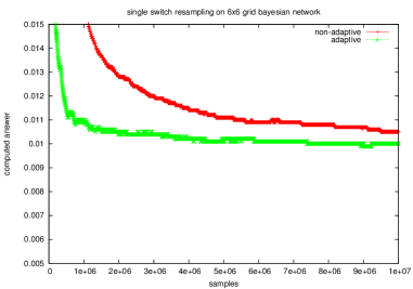
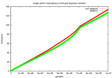
(a)	(b)

Figure 5: Bayesian Network, $6\times 6$ grid. (a) Conditional probability computed and (b) Running times as functions of sample size.

Hamming.

The Hamming code example is a PRISM program that generates a set of (4,3) Hamming codes. The evidence is a set of bits in the code with fixed values, and the query is the value of a non-evidence bit Moldovan et al. (2013). The data bits in the code were independent random variables, while the parity bits were computed from the data bits’ values. The answers computed by adaptive and non-adaptive samplers are given in Fig 6(a). The time taken by both the samplers is shown in Fig 6(b). In this example, the convergence of the adaptive MCMC is only a little better than that of the non-adaptive algorithm.

(a)	(b)

Figure 6: Hamming Code, 112 bits. (a) Condition probability computed and (b) Running times as functions of sample size.

Grammar.

This example checks a property of strings over open and closed parentheses. For any randomly generated string (not necessarily balanced), we define a “maximum nesting level” as the largest number of unmatched open parenthesis in a left-to-right scan of the string. Given that a randomly generated string has balanced parenthesis, this example evaluates the conditional probability of the query that determines whether a given random string has maximum nesting level of 3 or more. For the experiment, we fixed the length of strings to 200. The answers computed by adaptive and non-adaptive sampler are shown in Fig 7(a) and the times taken are shown in Fig 7(b). We used multi-switch resampling since the entire state space is not accessible via single switch resampling. Observe that adaptive sampling converges faster, although by a small margin; but adaptive sampling is almost twice as slow per iteration.

(a)	(b)

Figure 7: Nesting level in strings with balanced parenthesis. (a) Condition probability computed and (b) Running times as functions of sample size.

Reach.

The final set of examples are reachability queries in probabilistic acyclic graphs, of the form shown in Fig. 1. For the graph shown in Introduction, while computing $\mathtt{prob}(\mathtt{reach(a,d)}\mid\mathtt{reach(a,e)})$, the non-adaptive sampler rejects $8\%$ of the samples, while the non-adaptive one rejects $1.5\%$. Similar rejection rates were observed for larger randomly generated graphs as well. However, since the rejection rate of the non-adaptive sampler is low, there is no significant difference between the convergence of adaptive and non-adaptive samplers.

6 Discussion

Sampling-based approximate inference algorithms were proposed by Cussens (2000) for stochastic logic programs (SLP)s Muggleton et al. (1996). The algorithm defines an MCMC kernel on the derivations in an SLP. The technique used to propose the next state (i.e., derivation) involves backtracking one step at a time, stopping with a fixed probability given as a parameter. Once the backtracking stops, an alternate branch is sampled and resolution is continued to give next state. Our single-switch resampling technique different in that a single msw atom is chosen (uniformly at random) from the state and resampled. At a more fundamental level, our sampling technique is largely independent of the query evaluation process itself.

An MCMC technique has been proposed for Problog by Moldovan et al. (2013). It samples from explanations and makes use of a special algorithm to make the samples mutually exclusive. This incurs memory overhead (keeping track of possible worlds used for each explanation) as well as time overhead (to look back in a chain for previous uses of the same explanation. In contrast, we use Prolog-style evaluation to assure that the samples are pair-wise mutually exclusive.

Adaptive sequential rejection sampling proposed by Mansinghka et al. (2009) is an algorithm that explicitly adapts its proposal for generating samples for high dimensional graphical models. This algorithm requires the availability of a suitable factorization of the distribution with logarithmically few dependencies. Exact samples over a small set of variables are extended to exact samples over larger set of variables. The adaptation scheme described requires the complete knowledge of the factors in the distribution. Since PRISM programs represent logical as well as statistical knowledge, explicit knowledge may not even be available in our case. Consequently, our work does not rely on an explicit knowledge of factors.

We presented a MCMC technique for probabilistic logic programs that is largely independent of the manner in which queries are evaluated in the underlying logic programming systems. We defined an adaptive MCMC algorithm that adapts the probability distribution of individual switches and their instances to effectively explore the states of the Markov chain that are consistent with given evidence. We identified conditions under which a similar adaptation can be performed to enable independent samplers to draw more samples that are consistent with evidence. Preliminary experiments have shown both the potential and the limitations of this technique.

This paper focused on a generic MCMC method and adaptation, and did not consider the effect of resampling strategies. The order in which random processes are sampled may affect the convergence and hence the quality of inference. For instance, Decayed MCMC Marthi et al. (2002) samples processes based on a temporal order (resampling more recent processes more frequently). As future work, we plan extend our sampler to use an order based on programmer annotation; whether such annotations can be inferred from the program is an open problem. Finally, while sampling-based inference may be generally deployed, exact inference may still be feasible for queries with short derivations. Hence, an interesting direction of future work is to develop a hybrid inference technique that can combine exact and approximate inference based on programmer annotation. Such an inference technique can be seen as an analogue of the Rao-Blackwellized Particle Filtering method developed for Dynamic Bayesian Networks Doucet et al. (2000).

Appendix A Acceptance probability computation for MH sampler

Assume that the Markov chain is in state corresponding to assignment $\sigma$ and a proposal is made to transition to a different state corresponding to assignment $\sigma^{\prime}$. The set of switch/instance pairs in $\sigma$ can be divided into three disjoint sets: $\sigma_{1}=\{(s,i)|\sigma^{\prime}(s,i)=\bot\}$, $\sigma_{2}=\{(s,i)|\sigma^{\prime}(s,i)\neq\bot\text{ and }\sigma(s,i)\neq\sigma^{\prime}(s,i)\}$ and $\sigma_{3}=\{(s,i)|\sigma(s,i)=\sigma^{\prime}(s,i)\}$. The set of switch/instance pairs in $\sigma^{\prime}$ can be divided similarly. The probability of an assignment is simply the product of the probabilities of the outcomes of all switch/instance pairs in that assignment. The probability of an assignment $\sigma$ is denoted by $P(\sigma)$. We denote the number of switch/instance pairs in an assignment/sub-assignment $\sigma$ by $|\sigma|$. The acceptance probability for single switch non-adaptive resampling is

$$\frac{P(\sigma^{\prime})P(\sigma_{1})P(\sigma_{2})1/|\sigma^{\prime}|}{P(\sigma)P(\sigma^{\prime}_{1})P(\sigma^{\prime}_{2})1/|\sigma|}=\frac{P(\sigma^{\prime}_{1})P(\sigma^{\prime}_{2})P(\sigma^{\prime}_{3})P(\sigma_{1})P(\sigma_{2})1/|\sigma^{\prime}|}{P(\sigma_{1})P(\sigma_{2})P(\sigma_{3})P(\sigma^{\prime}_{1})P(\sigma^{\prime}_{2})1/|\sigma|}=\frac{|\sigma|}{|\sigma^{\prime}|}$$

Let the probability for forgetting switch in multi switch resampling be $p$. The acceptance probability can be computed as follows

$$\frac{P(\sigma^{\prime})p^{|\sigma_{2}|}P(\sigma_{2})P(\sigma_{1})\prod_{(s,i)\in\sigma_{3}}(1-p+pP(\sigma_{3}(s,i)))}{P(\sigma)p^{|\sigma^{\prime}_{2}|}P(\sigma^{\prime}_{2})P(\sigma^{\prime}_{1})\prod_{(s^{\prime},i^{\prime})\in\sigma^{\prime}_{3}}(1-p+p(\sigma^{\prime}_{3}(s^{\prime},i^{\prime})))}=1$$

In the case of adaptive sampling such simplifications are not possible. Let the adapted distribution be denoted by $P^{\prime}$. The probability of transition from $\sigma$ to $\sigma^{\prime}$ in case of single switch resampling is $P^{\prime}(\sigma^{\prime}_{1})P^{\prime}(\sigma^{\prime}_{2})/|\sigma|$. The acceptance probability is therefore computed as

$$\frac{P(\sigma^{\prime})P^{\prime}(\sigma_{1})P^{\prime}(\sigma_{2})1/|\sigma^{\prime}|}{P(\sigma)P^{\prime}(\sigma^{\prime}_{1})P^{\prime}(\sigma^{\prime}_{2})1/|\sigma|}=\frac{P(\sigma^{\prime}_{1})P(\sigma^{\prime}_{2})P^{\prime}(\sigma_{1})P^{\prime}(\sigma_{2})1/|\sigma^{\prime}|}{P(\sigma_{1})P(\sigma_{2})P^{\prime}(\sigma^{\prime}_{1})P^{\prime}(\sigma^{\prime}_{2})1/|\sigma|}$$

Finally we can show that the acceptance probability for multi switch resampling is

$$\frac{P(\sigma^{\prime})P^{\prime}(\sigma_{1})P^{\prime}(\sigma_{2})}{P(\sigma)P^{\prime}(\sigma^{\prime}_{1})P^{\prime}(\sigma^{\prime}_{2})}=\frac{P(\sigma^{\prime}_{1})P(\sigma^{\prime}_{2})P^{\prime}(\sigma_{1})P^{\prime}(\sigma_{2})}{P(\sigma_{1})P(\sigma_{2})P^{\prime}(\sigma^{\prime}_{1})P^{\prime}(\sigma^{\prime}_{2})}$$

References

- Andrieu et al. (2003) Andrieu, C., De Freitas, N., Doucet, A., and Jordan, M. 2003. An introduction to mcmc for machine learning. Machine learning 50, 1, 5–43.
- Brockwell and Kadane (2005) Brockwell, A. E. and Kadane, J. B. 2005. Identification of regeneration times in mcmc simulation, with application to adaptive schemes. Journal of Computational and Graphical Statistics 14, 2, 436–458.
- Cussens (2000) Cussens, J. 2000. Stochastic logic programs: Sampling, inference and applications. In Proceedings of the Sixteenth conference on Uncertainty in artificial intelligence. Morgan Kaufmann, 115–122.
- De Raedt et al. (2007) De Raedt, L., Kimmig, A., and Toivonen, H. 2007. ProbLog: A probabilistic prolog and its application in link discovery. In Proceedings of the 20th international joint conference on Artifical intelligence. 2462–2467.
- Doucet et al. (2000) Doucet, A., Freitas, N. d., Murphy, K. P., and Russell, S. J. 2000. Rao-Blackwellised particle filtering for dynamic bayesian networks. In Proceedings of the 16th Conference on Uncertainty in Artificial Intelligence (UAI). 176–183.
- Getoor and Taskar (2007) Getoor, L. and Taskar, B. 2007. Introduction to statistical relational learning. MIT press.
- Gilks et al. (1998) Gilks, W. R., Roberts, G. O., and Sahu, S. K. 1998. Adaptive markov chain monte carlo through regeneration. Journal of the American statistical association 93, 443, 1045–1054.
- Hastings (1970) Hastings, W. 1970. Monte carlo sampling methods using markov chains and their applications. Biometrika 57, 1, 97–109.
- Levin et al. (2009) Levin, D. A., Peres, Y., and Wilmer, E. L. 2009. Markov chains and mixing times. Amer Mathematical Society.
- Mansinghka et al. (2009) Mansinghka, V. K., Roy, D. M., Jonas, E., and Tenenbaum, J. B. 2009. Exact and approximate sampling by systematic stochastic search. In International Conference on Artificial Intelligence and Statistics. 400–407.
- Marthi et al. (2002) Marthi, B., Pasula, H., Russell, S., and Peres, Y. 2002. Decayed MCMC filtering. In Proceedings of the Eighteenth conference on Uncertainty in Artificial Intelligence (UAI). 319–326.
- Moldovan et al. (2013) Moldovan, B., Thon, I., Davis, J., and Raedt, L. D. 2013. Mcmc estimation of conditional probabilities in probabilistic programming languages. In ECSQARU. 436–448.
- Muggleton et al. (1996) Muggleton, S. et al. 1996. Stochastic logic programs. Advances in inductive logic programming 32, 254–264.
- Poole (1997) Poole, D. 1997. The independent choice logic for modelling multiple agents under uncertainty. Artificial Intelligence 94, 1, 7–56.
- Riguzzi and Swift (2011) Riguzzi, F. and Swift, T. 2011. The pita system: Tabling and answer subsumption for reasoning under uncertainty. Theory and Practice of Logic Programming (TPLP) 11, 4-5, 433–449.
- Roberts and Rosenthal (2007) Roberts, G. O. and Rosenthal, J. S. 2007. Coupling and ergodicity of adaptive markov chain monte carlo algorithms. Journal of applied probability 44, 2, 458–475.
- Roberts and Rosenthal (2009) Roberts, G. O. and Rosenthal, J. S. 2009. Examples of adaptive mcmc. Journal of Computational and Graphical Statistics 18, 2, 349–367.
- Sato and Kameya (1997) Sato, T. and Kameya, Y. 1997. Prism: a language for symbolic-statistical modeling. In In Proceedings of the 15th International Joint Conference on Artificial Intelligence (IJCAI 97). 1330–1335.
- Sutton and Barto (1998) Sutton, R. S. and Barto, A. G. 1998. Introduction to reinforcement learning. MIT Press.
- Swift et al. (2012) Swift, T., Warren, D. S., et al. 2012. The XSB logic programming system, Version 3.3. Tech. rep., Computer Science, SUNY, Stony Brook. http://xsb.sourceforge.net.
- Vennekens and Verbaeten (2003) Vennekens, J. and Verbaeten, S. 2003. A general view on probabilistic logic programming. In In Proceedings of BNAIC-03.