Fast Direct Methods for Gaussian Processes
Abstract
A number of problems in probability and statistics can be addressed using the multivariate normal (Gaussian) distribution. In the one-dimensional case, computing the probability for a given mean and variance simply requires the evaluation of the corresponding Gaussian density. In the -dimensional setting, however, it requires the inversion of an covariance matrix, , as well as the evaluation of its determinant, . In many cases, such as regression using Gaussian processes, the covariance matrix is of the form , where is computed using a specified covariance kernel which depends on the data and additional parameters (hyperparameters). The matrix is typically dense, causing standard direct methods for inversion and determinant evaluation to require work. This cost is prohibitive for large-scale modeling. Here, we show that for the most commonly used covariance functions, the matrix can be hierarchically factored into a product of block low-rank updates of the identity matrix, yielding an algorithm for inversion. More importantly, we show that this factorization enables the evaluation of the determinant , permitting the direct calculation of probabilities in high dimensions under fairly broad assumptions on the kernel defining . Our fast algorithm brings many problems in marginalization and the adaptation of hyperparameters within practical reach using a single CPU core. The combination of nearly optimal scaling in terms of problem size with high-performance computing resources will permit the modeling of previously intractable problems. We illustrate the performance of the scheme on standard covariance kernels.
Index Terms:
Gaussian process, covariance function, covariance matrix, determinant, hierarchical off-diagonal low-rank, direct solver, fast multipole method, Bayesian analysis, likelihood, evidenceI Introduction
Acommon task in probability and statistics is the computation of the numerical value of the posterior probability of some parameters conditional on some data using a multivariate Gaussian distribution. This requires the evaluation of
| (1) |
where is an symmetric, positive-definite covariance matrix. The explicit dependence of on particular parameters is shown here, and may be dropped in the proceeding discussion. In the one-dimensional case, is simply the scalar variance. Thus, computing the probability requires only the evaluation of the corresponding Gaussian. In the -dimensional setting, however, is typically dense, so that its inversion requires work as does the evaluation of its determinant . This cost is prohibitive for large .
In many cases, the covariance matrix is assumed to be of the form , where . This happens when the model for the data assumes some sort of uncorrelated additive measurement noise having variance in addition to some structured covariance described by the kernel . The function is called the covariance function or covariance kernel, which, in turn, can depend on additional parameters, . Covariance matrices of this form universally appear in regression and classification problems when using Gaussian process priors [49]. Because many covariance kernels are similar to those that arise in computational physics, a substantial body of work over the past decades has produced a host of relevant fast algorithms, first for the rapid application of matrices such as [31, 29, 21, 24, 64], and more recently on their inversion [30, 4, 7, 15, 21, 10, 43, 39]. We do not seek to further review the literature here, except to note that it is still a very active area of research.
Using the approach outlined in [4], we will show that under suitable conditions, the matrix can be hierarchically factored into a product of block low-rank updates of the identity matrix, yielding an algorithm for inversion. More importantly (and perhaps somewhat surprising), we show that our factorization enables the evaluation of the determinant, , in operations. Together, these permit the efficient direct calculation of probabilities in high dimensions. Previously existing methods for inversion and determinant evaluation were based on either rough approximation methods or iterative methods [13, 54, 55, 8, 17]. These schemes are particularly ill-suited for computing determinants. Although bounds exist for sufficiently random and diagonally dominant matrices, they are often inadequate in the general case [11]. We briefly review existing accelerated methods for Gaussian processes in Section II-D and present a cursory heuristic comparison with our covariance matrix factorization.
Gaussian processes are the tool of choice for many statistical inference or decision theory problems in machine learning and the physical sciences. They are ideal when requirements include flexibility for the modeling of continuous functions. However, applications are limited by the computational cost of matrix inversion and determinant calculation. Furthermore, the determinant of the covariance matrix is required for Gaussian process likelihood evaluations (i.e., computation of any actual value of the probability of the data under the covariance hyperparameters, or evidence). Existing linear algebraic schemes for direct matrix inversion and determinant calculation are prohibitively expensive when the likelihood evaluation is placed inside an outer optimization or Markov chain Monte Carlo (MCMC) sampling loop.
In this paper we will focus on describing and applying our new methods for handling large-scale covariance matrices (dense and full- or high-rank) to avoid the computational bottlenecks encounters in regression, classification, and other problems when using Gaussian process models. We motivate the algorithms by explaining where their need arises only in Gaussian process regression, but similar calculations are frequently encountered in other regimes under Gaussian process priors. Other applications, such as marginalization and adaptation of hyperparameters are relatively straightforward, and the computational bottlenecks of each are highly related.
The paper is organized as follows. Section II reviews some basic facts about Gaussian processes and the resulting formulas encountered in the case of a one-dimensional regression problem. Prediction, marginalization, adaptation of hyperparameters, and existing approximate accelerated methods are also discussed. Section III discusses the newly developed matrix factorization for Hierarchical Off-Diagonal Low-Rank (HODLR) matrices, for which factorization requires only work. Subsequent applications of the operator and its inverse scale as . Many popular covariance functions used for Gaussian processes yield covariance matrices satisfying the HODLR requirements. While other hierarchical methods could be used for this step, we focus on the HODLR decomposition because of its simplicity and applicability to a wide range of covariance functions. We would like to emphasize that the algorithm will work for any covariance kernel, but the scaling of the algorithm might not be optimal; for instance, if the covariance kernel has a singularity or is highly oscillatory without damping. Further, in Section IV, we show that the determinant of an HODLR decomposition can be computed in operations. Section V contains numerical results for our method applied to some standard covariance functions for data embedded in varying dimensions. Finally, in Section VI, we summarize our results and discuss any shortcomings and other applications of the method, as well as future avenues of research.
The conclusion contains a cursory description of the corresponding software packages in C++ and Python which implement the numerical schemes of this work. These open-source software packages have been made available since the time of submission.
II Gaussian processes and regression
In the past two decades, Gaussian processes have gained popularity in the fields of machine learning and data analysis for their flexibility and robustness. Often cited as a competitive alternative to neural networks because of their rich mathematical and statistical underpinnings, practical use in large-scale problems remains out of reach due to computational complexity. Existing direct computational methods for manipulations involving large-scale covariance matrices require calculations. This causes regression/prediction, parameter marginalization, and optimization of hyperparameters to be intractable problems. This scaling can be reduced in special cases via several approximation methods, discussed in Section II-D, however for dense, highly coupled covariance matrices no suitable direct methods have been proposed. Here, by direct method we mean one that constructs the inverse and determinant of a covariance matrix to within some pre-specified numerical tolerance directly instead of iteratively. The matrix inverse can then be stored for use later, much as standard or factorizations. The numerical tolerance can be measured in the spectral or Frobenius norms, and our algorithm is able to easily achieve approximations on the order of . Often, near machine precision () is attainable.
The following sections contain an overview of regression via Gaussian processes and the large computational tasks that are required at each step. The one-dimensional regression case is discussed for simplicity, but similar formulae for higher dimensions and classification problems are straightforward to derive. In higher dimensions, the corresponding computational methods scale with the same asymptotic complexity, albeit with larger constants. For a thorough treatment of regression using Gaussian processes, see [49, 42].
The canonical linear regression problem we will analyze assumes a model of the form
| (2) |
where is some form of uncorrelated measurement noise. Given a dataset , the goal is to infer , or equivalently some set of parameters that depends on. We will enforce the prior distribution of the unknown function to be a Gaussian process,
| (3) |
where is some admissable covariance function ( corresponds to positive definite covariance matrices), possibly depending on some unknown hyperparameters, and is the expected mean of . The task of fitting hyperparameters is discussed in Sections II-B and II-C of the paper. Table I lists some of the frequently used covariance functions for Gaussian processes.
| Name | Covariance function |
|---|---|
| Ornstein-Uhlenbeck | |
| Gaussian | |
| Matérn family | |
| Rational Quadratic |
II-A Prediction
One of the main uses for the previous model (especially in machine learning) is to predict, with some estimated confidence, for some new input data point . This is equivalent to calculating the conditional distribution . We will not assume any parametric form of , and enforce structure only through the observed data and the choice of the mean function and covariance function . Additionally, for the time being, assume that is fixed (i.e., hyperparameters are either fixed or absent). Given the data and , it is easy to show that the conditional distribution (likelihood) of is given by
| (4) |
where the mean vector and covariance matrix are:
| (5) | ||||
The conditional distribution of a predicted function value, , can then be calculated as
| (6) |
with
| (7) | ||||
In the previous formulas, for the sake of simplicity, we have assumed that the mean function . The vector is the column vector of covariances between and all the known data points , and [49]. We have therefore reduced the problem of prediction and confidence estimation (in the expected value sense) down to matrix-vector multiplications. For large , the cost of inverting the matrix is expensive, with direct methods for dense systems scaling as . A direct algorithm for the rapid inversion of this matrix is one of the main contributions of this paper.
II-B Hyperparameters and marginalization
As mentioned earlier, often the covariance function used to model the data , depends on some set of parameters, . For example, in the case of a Gaussian covariance function
| (8) |
the column vector of hyperparameters is given by .
Often hyperparameters correspond to some physically meaningful quantity of the data, for example, a decay rate or some spatial scale. In this case, these parameters are fixed once and for all according to the specific physics or dynamics of the model. On the other hand, hyperparameters may be included for robustness or uncertainty quantification and must be marginalized (integrated) away before the final posterior distribution is calculated. In this case, for relevant hyperparameters and nuisance parameters , in order to compute the evidence one must compute marginalization integrals of the form
| (9) |
where is a covariance matrix corresponding to the Gaussian process prior and is some prior on . If there are nuisance parameters, this is an -dimensional integral whose numerical integration requires quadrature nodes, where is roughly the number of quadrature nodes needed for one-dimensional marginalization. Unless and can be calculated rapidly for varying samples of the nuisance parameters, the direct calculation of this integral is not possible. Rapid algorithms for constructing and would allow for the direct marginalization of nuisance parameters, thereby directly constructing the probability of the data, or the marginal evidence. This is in contrast with several existing approximate Monte Carlo methods for computing the above integral (e.g. importance sampling, MCMC, etc.), which are not direct, and which converge with only half-order accuracy (i.e. the numerical accuracy of the integral only decreases as , where is the number of Monte Carlo samples). These sampling methods may decrease the number of inversions of for varying parameters, but do not completely avoid this cost.
II-C Adaptation of hyperparameters
Alternatively, there exist situations in which the hyperparameters do not arise out of physical considerations, but rather one would like to infer them as best fit parameters. This entails minimizing some regression norm with respect to the parameters,
or rather maximizing a parameter likelihood function (point estimation using a Bayesian framework):
In either case, some manner of non-linear optimization must be performed because of the non-linear dependence of every entry of the covariance matrix on the hyperparameters .
Regardless of the type of optimization scheme selected, several evaluations of the evidence, likelihood, and/or Gaussian regression must be performed – each of which requires evaluation of the inverse of the covariance matrix, . In order to achieve the maximum rate of convergence of these opimization algorithms, the full likelihood (or evidence) is required, i.e. the numerical value of the determinant of is need. Unless the determinant and inverse can be re-calculated and applied to the data rapidly, optimizing over all possible ’s is not a computationally tractable problem. We skip the discussion of various optimization procedures relevant to the adaptation of hyperparameters in Gaussian processes [49] , but only point out that virtually all of them require the re-computation of the inverse covariance matrix .
II-D Accelerated methods
A variety of linear-algebraic methods have been proposed to accelerate either the inversion of , the computation of its determinant, or both. If is of low-rank, say , then it is straightforward to compute and using the the Sherman-Morrison-Woodbury formula [61, 53, 36] and the Sylvester determinant theorem [1] in operations. However, unless an analytical form of the low-rank property of the covariance kernel is known, some type of dense numerical linear algebra must be performed. Usually, constructing general low-rank approximations to matrices requires at least operations, where is the numerical rank of the matrix. By numerical rank we loosely mean that there are (normalized) singular values larger than some specified precision, . This definition of numerical rank is consistent with spectral norm, and closely related to the Frobenius norm.
Almost all of the dense matrix low-rank approximations construct some suitable factorization (approximation) of :
| (10) |
where one can think of as compressing the action of onto a subset of points , as the covariance kernel acting on that subset, and as interpolating the result to the full set of points [55, 56, 54, 45].
Iterative methods can also be applied. These are particularly effective when there is a fast method to compute the necessary matrix-vector products. For Gaussian covariance matrices, this can be accomplished using the fast Gauss transform [29] and its higher-dimensional variants using -trees (see, for example, [63, 52]). Alternatively, when is a convolution kernel and the data are equispaced, the Fast Fourier Transform (FFT) can be used to accelerate the matrix vector product [18]. For non-equispaced data, non-uniform Fast Fourier Transforms (NUFFTs) are applicable [19, 20, 28]. As mentioned in the introduction, analysis-based fast algorithms can also be used for specific kernels [17] or treated using the more general “black-box” or “kernel-independent” fast multipole methods [21, 24, 64].
In some instances, the previously described linear algebraic or iterative methods can be avoided all-together if an analytical decomposition of the kernel is known. For example, much of the mathematical machinery needed to develop the fast Gauss transform [29] relies on careful analysis of generating functions (or related expansions) of the Gaussian kernel. For example,
| (11) |
expresses the Gaussian as a sum of separated functions in , , centered about , scaled by , and where is the degree Hermite function. Similar formulas, often referred to as addition formulas or multipole expansions in the physics literature, can be derived for other covariance kernels. As another example, one could build a low-rank representation of covariance matrices generated by the Matérn kernel using formulas of the form:
| (12) |
where , are complex variables for which and is the modified Bessel function of the second kind or order . See [46, 60] for a full treatment of formulas of this type. Relationships such as the previous ones lead (almost) directly to fast algorithms for the forward application of the associated covariance matrices. Directly building the inverse matrix (and evaluating the determinant) is more complicated.
Before we move on, there are several other accelerated methods which are popular in the Gaussian process community (namely greedy approximations, sub-sampling, and the Nyström method) [49]. We would like to briefly describe the accelerations that can be obtained by interpreting Gaussian processes via a state-space model [51, 37, 57].
Stochastic linear differential equations (causal, and driven by Gaussian noise) and state-space models are intimately connected with Gaussian processes and (stationary) covariance functions via the Wiener-Khintchine theorem [16]. In particular, this observation allows one to construct spectral density approximations to stationary covariance kernels which in turn give rise to a corresponding state-space process. This process can then be analyzed using Kalman filters and other smoothers, which often have linear computational complexity time for single point inference [37], [40]. The accuracy of this inference lies in the quality of the spectral density approximation, which is usually expressed as a rational function. This finite-rank spectral density approximation via rational functions can be interpreted much in the same way as approximating the Gaussian process covariance matrix as in equation (10) – once this finite-rank approximation is constructed, the resulting matrix inversion scales as by the Sherman-Morrison-Woodbury formula (see Section III). Applying state-space models to parameter inference problems, instead of smoothing or functional inference problems, is more subtle but several methods from signal processing are useful. For a clear exposition on this topic, see [51, 12]. Often the asymptotic computational cost of the state-space model analysis will be similar to the algorithm of this paper because both methods are using rank considerations to approximate the covariance structure – the algorithm of this paper uses a spatial-hierarchical method, whereas fast state-space methods use a spectral approximation of temporal data.
One last theme for increasing the scalability of Gaussian processes to big data sets is to introduce some notion of sparsity [38, 45]. Many of the previous accelerated methods can be interpreted as introducing sparsity at the covariance kernel level – i.e. by approximating the matrix as a finite rank operator. The resulting approximation is dense, but data-sparse. Alternatively, one may introduce sparsity at the level of the actual matrix by thresholding small elements away from the diagonal. The resulting may retain high (or full) numerical rank, but the actual matrix is sparse, thereby enabling sparse matrix algebra to be performed which has reached a high level of acceleration in modern computing environments. Sparsity may also be introduced by the inclusion of data-generating latent variables (related to the state-space interpretation of Gaussian processes), similar to hidden Markov models [38, 12, 51].
It should be noted that all of the previous methods for accelerating Gaussian process calculations involve some sort of approximation. Depending on the method, either the resulting covariance matrix is approximated (using a low-rank factorization) or the actual covariance kernel is approximated (using a low-rank representation, or by approximating the actual Gaussian process by a finite-rank chain, as in the case of the state-space models). In each case, the analysis of the approximating Gaussian process is different because the approximation take place at different levels in the mathematics. Our accelerated direct method, which is described in the next section, makes an approximation at the level of the covariance matrix. This is akin to viewing the covariance matrix as a continuous linear operator, and not an arbitrary data matrix. Often this approximation is negligible as it is near to machine precision in finite digit arithmetic.
Lastly, the evaluation of determinants is a somewhat different matter. Most of the previously described accelerated approximations in this section are unable to evaluate the determinant in less than time since this is equivalent to constructing some matrix factorization or all of the eigenvalues. Taylor series approximations [47] and Monte Carlo methods have been suggested [9], as well as conjugate gradient-type methods combined with trace estimators [17]. For additional approximation methods, see the text [49]. In general, however, it is difficult to obtain accurate values for the determinant in a robust and reliable manner. Thus, the development of a fast, accurate, and direct method is critical in making large-scale Gaussian process modeling useful for for exact inference problems.
III Hierarchical matrices
A large class of dense matrices, for example, matrices arising out of boundary integral equations [65], radial basis function interpolation [4], kernel density estimation in machine learning, and covariance matrices in statistics and Bayesian inversion [6, 5], can be efficiently represented as data-sparse hierarchical matrices. After a suitable ordering of columns and rows, these matrices can be recursively sub-divided and certain sub-matrices at each level can be well-represented by low-rank matrices.
We refer the readers to [34, 35, 27, 33, 10, 15, 14, 2] for more details on this approach. Depending on the subdivision structure and low-rank approximation technique, different hierarchical decompositions exist. For instance, the fast multipole method [31] accelerates the calculation of long-range gravitational forces for -body problems by hierarchically compressing the associated matrix operator using low-rank considerations. The algorithm of this paper makes use of sorting data points according to a -tree, which has the same formalism in arbitrary dimension. The data is sorted recursively, one dimension at a time, yielding a data structure which can be searched in at most time, and often much faster. Once the sorting is completed, the data points can be globally re-ordered according to, for example, a -order or -curve. It is this ordering which generates a correspondence between individual data points and matrix columns and rows. Based on the particular covariance kernel and the data structure used (an adaptive versus a uniform sorting), the resulting algorithm will perform slightly differently, but with the same asymptotic scaling.
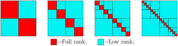
In this article, we will be working with the class of hierarchical matrices known as Hierarchical Off-Diagonal Low-Rank (HODLR) matrices [4], though the ideas extend for other classes of hierarchical matrices as well. As the name suggests, this class of matrices has off-diagonal blocks that are efficiently represented in a recursive fashion. A graphical representation of this class of matrices is shown in Figure 1. Each block represents the same matrix, but viewed on different hierarchical scales to show the particular rank structure.
We first give an example of a simple two-level decomposition for real symmetric matrices, and then describe the arbitrary-level case in more detail. In a slight abuse of notation, in order to be consistent with previous sources describing HODLR matrices, we will refer to the decomposition of a matrix , which is not necessarily the same as previously mentioned in the covariance matrix case, namely in .
Algebraically, a real symmetric matrix is termed a two-level HODLR matrix, if it can be written as:
| (13) |
with the diagonal blocks given as
| (14) | ||||
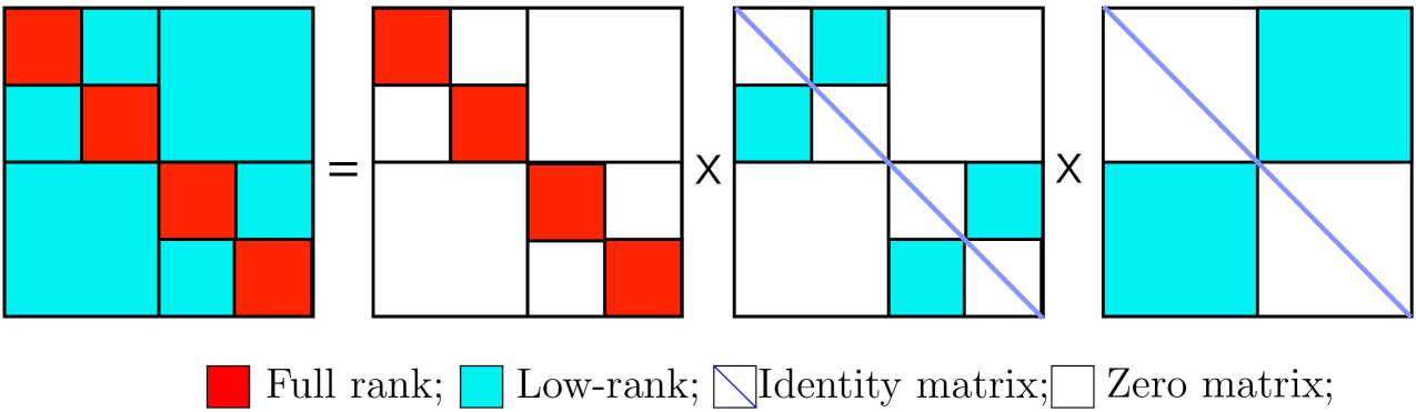
where the , matrices are matrices and . In practice, the rank of the , matrices will fluctuate slightly based on the desired accuracy of the approximation. In general, all off diagonal blocks of all factors on all levels can be well-represented by a low-rank matrix, i.e., on each level, are tall and thin matrices. It is easy to show that the matrix structure given in equations (13) and (14) can be manipulated to provide a factorization of the original matrix as a product of matrices, one of which is block-diagonally dense, and the rest of which are block-diagonal low-rank updates to the identity matrix. This is shown in Figure 2.
The above is merely a description of the structure of matrices which meet the HODLR requirements, but not a description of how to actually construct the factorization. There are two aspects which need to be discussed: (i) constructing the low-rank approximations of all the off-diagonal blocks, and (ii) using these low-rank approximations to recursively build a factorization of the form shown in Figure 2. We now describe several methods for constructing the low-rank approximations in the next section.
III-A Fast low-rank approximation of off-diagonal blocks
The first key step is to have a computationally efficient way of obtaining the low-rank factorization of the off-diagonal blocks. Given any matrix , the optimal low-rank approximation (in the least-squares sense) is obtained using the singular value decomposition (SVD) [25]. The downside of using the SVD is that the computational cost of direct factorizations scales as , where is the numerical rank of the matrix. In practice, is obtained on-the-fly such that the factorization is accurate to some specified precision . For our algorithm to be computationally tractable, we need a fast low-rank factorization. More precisely, we need algorithms that scales at most as to obtain a rank factorization of a matrix. Thankfully, there has recently been tremendous progress in obtaining fast low-rank factorizations of matrices. These techniques can be broadly classified as either analytic or linear-algebraic techniques.
If the matrix entries are obtained as evaluations from a smooth function, as is the case for most of the covariance matrices in Gaussian processes, we can rely on approximation theory based analytic techniques like interpolation, multipole expansion, eigenfunction expansion, Taylor series expansions, etc. to obtain a low-rank decomposition. In particular, if the matrix elements are given in terms of a smooth function , as in the Gaussian process case,
| (15) |
then polynomial interpolation methods can be used to efficiently approximate the matrix with near spectral accuracy. Barycentric interpolation formulae such as those recently discussed by Townsend and Trefethen and others [58, 59] serve to effectively factorize into
| (16) |
where is a matrix obtained by sampling the function at suitable chosen nodes, e.g. Chebyshev interpolation nodes. The matrices , are then obtained via straightforward interpolation formulas. The accuracy of the approximation can be estimated from spectral analysis of the interpolating Chebyshev polynomial, and the approximation can be computed in time.
On the other hand, if there is no a-priori information of the matrix, then linear-algebraic methods provide an attractive way of computing fast low-rank decompositions. These include techniques like pseudo-skeletal approximations [26], interpolatory decomposition [21], randomized algorithms [23, 41, 62], rank-revealing [44, 48], adaptive cross approximation [50, 66] (which is a minor variant of partial-pivoted ), and rank-revealing [32]. Though purely analytic techniques can be faster since many operations can be pre-computed, algebraic techniques are attractive for constructing black-box low-rank factorizations. The algorithm of this paper relies on an implementation of approximate partial-pivoted , which we will now discuss.
Briefly, we construct factorizations of off-diagonal blocks via a partial-pivoted decomposition which executes in time. Heuristically, this factorization constructs a series of rank-one matrices whose sum approximates the original matrix, i.e. we wish to write
| (17) |
The vectors , are computed from the columns and rows of .
The linear complexity is achieved by checking the resulting approximation against only a sub-sampling of the original matrix. If the underlying matrix (covariance kernel) is sufficiently smooth, then this sub-sampling error estimation will result in an approximation which is accurate to near machine precision. For other matrices or covariance kernels which are highly oscillatory or contain small-scale structure, this method will not scale and will likely yield a less-accurate approximation. In this case, analytic methods are preferable as they will be more efficient and provide suitable high-accuracy approximations. We omit a pseudo-code description of this algorithm, as it is a well-know linear algebra procedure, and instead refer to Section 2.2, Algorithm 6 of [50].
The next section presents the fast matrix factorization of the entire covariance matrix once the low-rank decomposition of the off-diagonal blocks has been obtained using one of the above mentioned techniques. We offer a concise, but complete description of the factorization in order to make the exposition self-contained. For a longer and more detailed discussion of the material, see [4].
III-B HODLR matrix factorization
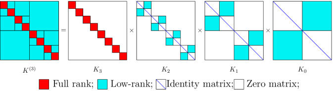
The overall idea behind the factorization of an , -level (where ) HODLR matrix as described in [4] is to factor it as a product of block diagonal matrices,
| (18) |
where, except for , is a block diagonal matrix with diagonal blocks, each of size . More importantly, each of these diagonal blocks is a low-rank update to the identity matrix. The first factor is formed from dense block diagonal sub-matrices of the original matrix, . Aside from straightforward block-matrix algebra, the main tool used in constructing this factorization is the Sherman-Morrison-Woodbury formula [61, 53, 36]. To simplify the notation assume for a moment that is an matrix, where for some integer . For example, a two-level HODLR matrix described in equations (13) and (14) can be factorized as:
| (19) |
where is the identity matrix, and the matrices are low-rank. Similarly, Figure 3 graphically depicts the factorization of a level HODLR matrix.
In the case of a one-level factorization, we can easily write down the computation. Let the matrix be:
| (20) |
where we assume that , have been computed using one of the algorithms of the previous section. Then the only step in the decomposition is to factor out the terms , , giving:
| (21) |
We see that the computation involved was to merely apply the inverse of the dense block diagonal factor to the corresponding rows in the remaining factor. Furthermore, since the matrix was low-rank, so is . Unfortunately, a one-level factorization such as this is still quite expensive: it required the direct inversion of , , each of which are matrices. The procedure must be done recursively across levels in order to achieve a nearly optimal algorithm.
|
|
(22) |
Before describing the general scheme, we give the full two-level factorization using the notation of equations (13) and (14). The full factorization in this two-level scheme is given in equation (22) (spanning two columns on the proceeding page). The matrices and appearing in the off-diagonal expressions are given by:
| (23) | ||||
This factorization is an indication of how to construct the ultimate -level factorization as it only required the direct construction of the inverse of dense matrices of size . If this procedure is repeated recursively, the only dense inversions required are of matrices.
At first glance, it may look as though the computation of , is expensive, and will scale as . However, these matrices are of the form:
| (24) |
If the inverses of , are known (and they are in this case, they were computed on a finer level), and , are low-rank matrices, then the inverse of the full matrix can be computed rapidly using the Sherman-Morrison-Woodbury formula:
If is of small rank, then the inner inverse can be computed very rapidly.
To summarize, see Figure 4 for rough pseudo-code describing how to construct a general -level HODLR factorization. We avoid too much index notation, please see [4] for a full detailed algorithm.
This pseudo-code computes a factorization of the original matrix . We have not yet computed the inverse . The inverse can be computed by directly applying the Sherman-Morrison-Woodbury formula to each term in the factorization
| (25) |
Since each term is block diagonal or a block diagonal low-rank update to the identity matrix, the inverse factorization can be computed in time.
Before moving on we would like to point out that in the case where the data points at which the kernel is to be evaluated at are not approximately uniformly distributed, the performance of the factorization may suffer, but only slightly. A higher level of compression could be obtained in the off-diagonal blocks if the hierarchical tree structure is constructed based on spatial considerations instead of point count, as is the case with some -tree implementations.
The next section gives a brief estimate of the computational complexity of constructing a HODLR-type factorization.
III-C Computational complexity
Constructing a HODLR-type factorization can be split into two main steps: (i) computing the low-rank factorization of all off-diagonal blocks, and (ii) using these low-rank approximations to recursively factor the matrix into roughly pieces.
For an matrix which admits the HODLR structure, as shown in, Figure 1, there are approximately , where is the size of the diagonal block on the finest level (this is a user-defined parameter). Ignoring the diagonal blocks, this means there are two blocks of size , four blocks of size , etc. Finding the low-rank approximation of an off-diagonal block using cross approximation requires flops, where is the -rank of the sub-matrix. Constructing all such factorizations requires .
Once the approximations are obtained, the matrix must be pulled apart into its HODLR factorization. Let us remember that there are levels in the HODLR structure. In order to factor (the matrix of dense block diagonals), as in equation (18), out of the original matrix , we must apply the inverse of the corresponding block diagonal to all the left low-rank factors, , as in equations (21) - (23). In general, a inverse must computed and applied to all left low-rank factors, of which there are . The inverse calculation is , and the subsequent application is , , which dominates the inverse calculation. There are such applications, yielding the cost for only the first factorization level to be . Applying the same reasoning as each subsequent factor , , along with the complexity result,
| (26) |
yields a total complexity for the factorization stage of . The factors of , have been dropped as it is assumed that .
Given a HODLR-type factorization, it is straightforward to show that the computational complexity of determining the inverse scales as . There are factors, and since each level is constructed as low-rank updates to the identity, invoking the Sherman-Morrison-Woodbury formula yields the inverse in time. This gives a total runtime of .
IV Determinant computation
As discussed earlier, once the HODLR factorization has been obtained, Sylvester’s determinant theorem [1] enables the computation of the determinant at a cost of operations. This computationally inexpensive method for direct determinant evaluation enables the efficient direct evaluation of probabilities. We now briefly review the algorithm used for determinant evaluation.
Theorem IV.1 (Sylvester’s Determinant Theorem).
If and , then
where is the identity matrix. In particular, for a rank update to the identity matrix,
Remark IV.2.
The computational cost associated with computing the determinant of a rank update to the identity is . The dominant cost is computing the matrix-matrix product .
Furthermore, we recall two basic facts regarding the determinant. First, the determinant of a block diagonal matrix is the product of the determinants of the individual blocks of the matrix. Second, the determinant of a square matrix is completely multiplicative over the set of square matrices, that is to say,
| (27) |
Using the HODLR factorization in equation (18) and these two facts, we have:
| (28) |
Each of the determinants on the right hand side of equation (28) can be computed as a product of the determinants of diagonal blocks. Each of these diagonal blocks is a low-rank perturbation to the identity, and hence, the determinant can be computed using Sylvester’s Determinant Theorem IV.1. It is easy to check that the computational cost for each of the determinants is , therefore the total computational cost for obtaining is , and we recall that .
V Numerical results
In this section, we discuss the performance of the previously described algorithm for the inversion and application of covariance matrices , as well as the calculation of the normalization factor, i.e., the determinant . Detailed results for -dimensional datasets , where each is a point in one, two, and three dimensions, are provided for the Gaussian and multiquadric covariance kernels. We also provide benchmarks in one dimension for covariance matrices constructed from exponential, inverse multiquadric, and biharmonic covariance functions. Unless otherwise, stated, all the proceeding numerical experiments have been run on a MacBook Air with a 1.3GHz Intel Core i5 processor and 4 GB 1600 MHz DDR3 RAM. In all these cases, the matrix entry is given as
where is a particular covariance function evaluated at two points, and . It should be noted that in certain cases, the matrix with entries might itself be a rank deficient matrix and that this has been exploited in the past to construct fast schemes. However, this is not always the case, for instance, if the covariance function is an exponential. In this situation, the rank of is in fact full-rank. Even if the matrix were to be formally rank deficient, in practice, the rank might be very large whereas the ranks of the off-diagonal blocks in the hierarchical structure are very small. Another major advantage of this hierarchical approach is that it is applicable to a wide range of covariance functions and can be used in a black-box, plug-and-play, fashion.
In each of the following tables, timings are provided for the assembly, factorization, and inversion of the covariance matrix (denoted by the columns Assembly, Factor, and Solve). Assembly of the matrix refers to computing all of the low-rank factorizations of the off-diagonal blocks (including the time required to construct a -tree on the data), and Factor refers to computing the level factorization described earlier. The time for computing the determinant of the matrix is given in the Det. column, and the error provided is approximately the relative precision in the solution to a test problem , where was generated a priori from the known vector .
V-A Gaussian covariance
Here the covariance function, and the corresponding entry of , is given as
| (29) |
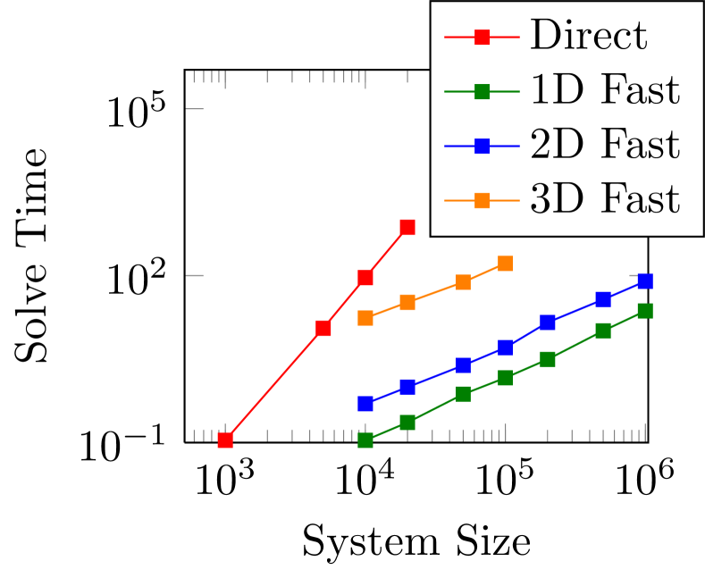
where , are points in one, two, or three dimensions. The results for the Gaussian covariance kernel have been aggregated in Table II. Scaling of the algorithm for data embedded in one, two, and three dimensions is compared with the direct calculation in Figure 5.
| One-dimensional data | Two-dimensional data | Three-dimensional data | |||||||||||||
| Assembly | Factor | Solve | Det. | Error | Assembly | Factor | Solve | Det. | Error | Assembly | Factor | Solve | Det. | Error | |
V-B Multiquadric covariance matrices
Covariance functions of the form
| (30) |
are known as multiquadric covariance functions, one class of frequently used radial basis functions. Analogous numerical results are presented below in one, two, and three dimensions as were in the previous section for the Gaussian covariance function. Table III contains the results. Scaling is virtually identical to the Gaussian case, and we omit the corresponding plot.
| One-dimensional data | Two-dimensional data | Three-dimensional data | |||||||||||||
| Assembly | Factor | Solve | Det. | Error | Assembly | Factor | Solve | Det. | Error | Assembly | Factor | Solve | Det. | Error | |
| 0.08 | 0.13 | 0.006 | 0.02 | 0.77 | 0.86 | 0.022 | 0.04 | 19.0 | 23.2 | 0.135 | 1.32 | ||||
| 0.11 | 0.22 | 0.011 | 0.03 | 1.41 | 1.42 | 0.042 | 0.06 | 38.7 | 45.1 | 0.276 | 1.65 | ||||
| 0.34 | 0.65 | 0.030 | 0.13 | 3.31 | 3.43 | 0.082 | 0.15 | 87.8 | 97.8 | 0.578 | 2.28 | ||||
| 0.85 | 1.44 | 0.059 | 0.22 | 6.54 | 6.95 | 0.177 | 0.31 | 164 | 195 | 1.24 | 3.84 | ||||
| 1.56 | 3.12 | 0.147 | 0.44 | 14.1 | 15.9 | 0.395 | 0.59 | ||||||||
| 4.72 | 8.33 | 0.363 | 0.94 | 38.2 | 42.1 | 1.12 | 1.69 | ||||||||
| 10.9 | 17.1 | 0.814 | 1.94 | 79.9 | 90.3 | 2.38 | 3.39 | ||||||||
V-C Exponential covariance
Covariances functions of the form
| (31) |
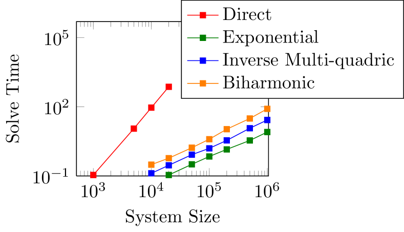
are known as exponential covariance functions. One-dimensional numerical results are presented in Table IV. Figure 6 compares scaling for various kernels.
| Time taken in seconds | |||||
|---|---|---|---|---|---|
| Assembly | Factor | Solve | Det. | Error | |
| 0.13 | 0.06 | 0.003 | 0.02 | ||
| 0.23 | 0.11 | 0.008 | 0.03 | ||
| 0.64 | 0.32 | 0.020 | 0.10 | ||
| 1.41 | 0.70 | 0.039 | 0.23 | ||
| 2.86 | 1.42 | 0.076 | 0.42 | ||
| 8.63 | 3.47 | 0.258 | 0.67 | ||
| 18.8 | 8.05 | 0.636 | 1.35 | ||
V-D Inverse Multiquadric and Biharmonic
The inverse multiquadric and biharmonic kernel (also known as the thin plane spline) are frequently used in radial basis function interpolation and kriging in geostatistics. These kernels are given by the formulae
| (32) | ||||
respectively. Timing results are presented in Tables V and VI, and comparison with the exponential kernel is shown in Figure 6.
| Time taken in seconds | |||||
|---|---|---|---|---|---|
| Assembly | Factor | Solve | Det. | Error | |
| 0.11 | 0.13 | 0.006 | 0.02 | ||
| 0.17 | 0.29 | 0.017 | 0.04 | ||
| 0.47 | 0.84 | 0.037 | 0.12 | ||
| 1.07 | 1.58 | 0.072 | 0.21 | ||
| 2.18 | 3.49 | 0.158 | 0.44 | ||
| 6.43 | 11.8 | 0.496 | 0.71 | ||
| 14.2 | 26.8 | 1.02 | 1.49 | ||
| Time taken in seconds | |||||
|---|---|---|---|---|---|
| Assembly | Factor | Solve | Det. | Error | |
| 0.28 | 0.31 | 0.015 | 0.03 | ||
| 0.61 | 0.59 | 0.028 | 0.06 | ||
| 1.62 | 1.68 | 0.067 | 0.15 | ||
| 3.61 | 3.93 | 0.123 | 0.34 | ||
| 8.03 | 10.7 | 0.236 | 0.65 | ||
| 26.7 | 31.2 | 0.632 | 1.41 | ||
| 51.3 | 81.9 | 1.28 | 3.40 | ||
V-E Scaling in high dimensions
In this section we report results on the scaling of the algorithm described in this paper when the data (independent variables, ) lie in high Euclidean dimensions. We perform two experiments. First, we run our algorithm on data lying in the hypercube for various values of . In this scenario, we actually see an increase in computational speed and accuracy as is increased after some point. These results are reported in Table VII. However, this is not a fair result. As increases, the expected value of increases, causing, at least in the case of an unscaled Gaussian covariance kernel, for many matrix entries to be very close to zero.
The second experiment was with the same set of parameters, except the data are located in the scaled hypercube, . These results are reported in Table VIII. This is equivalent to rescaling Euclidean distance, or rescaling the covariance kernel. We see that the scalings for this experiment saturate once due to the fact that we are not increasing the number of data points along with . For fixed , the data become very sparse as increases and the ranks of the off-diagonal blocks in the associated covariance matrix remain the same. What we mean to say by this is that points in a ten-dimensional space is massively under-sampling any sort of spatial structure, this is equivalent to grid of about two or three points per dimension (). Running the algorithm with this type of data is equivalent to doing dense linear algebra since the ranks of all off-diagonal blocks are close to full. This is a manifestation of the curse of dimensionality. However, it’s possible that one may encounter both types of data (scaled vs. unscaled) in real-world situations.
These experiments were run on a faster laptop, namely a MacBook Pro with a 3.0GHz Intel Core i7 processor and 16 GB 1600 MHz DDR3 RAM. No sophisticated software optimizations were made.
| Time taken in seconds | ||||||
|---|---|---|---|---|---|---|
| Dim | Assembly | Factor | Solve | Det. | Error | |
| 1 | 0.02 | 0.087 | 0.002 | 0.001 | ||
| 2 | 1.17 | 2.043 | 0.027 | 0.014 | ||
| 4 | 9.67 | 21.25 | 0.073 | 0.088 | ||
| 8 | 10.4 | 7.773 | 0.041 | 0.039 | ||
| 16 | 0.09 | 0.168 | 0.002 | 0.002 | ||
| 32 | 0.15 | 0.061 | 0.004 | 0.001 | ||
| 64 | 0.21 | 0.059 | 0.001 | 0.001 | ||
| Time taken in seconds | ||||||
|---|---|---|---|---|---|---|
| Dim | Assembly | Factor | Solve | Det. | Error | |
| 1 | 0.02 | 0.087 | 0.002 | 0.001 | ||
| 2 | 0.70 | 1.157 | 0.017 | 0.005 | ||
| 4 | 33.6 | 108.2 | 0.165 | 0.360 | ||
| 8 | 40.8 | 138.4 | 0.186 | 0.359 | ||
| 16 | 41.9 | 138.7 | 0.182 | 0.358 | ||
| 32 | 43.4 | 174.1 | 0.174 | 0.354 | ||
| 64 | 42.2 | 142.2 | 0.181 | 0.346 | ||
V-F Regression performance
In this section we demonstrate the relationship between various parameters in our algorithm and regression performance. The two main parameters that need to be set in our algorithm are the factorization precision (see Figure 4) and the maximum size of the smallest sub-matrix on the finest level, . For a fixed , changing does not affect the (root-mean-square error) of the regression (up to machine precision errors), it merely affects the overall runtime. For sufficiently large , the scheme ceases to be a multi-level algorithm. We merely state this as a fact, and do not report the data. We set in the following numerical experiment.
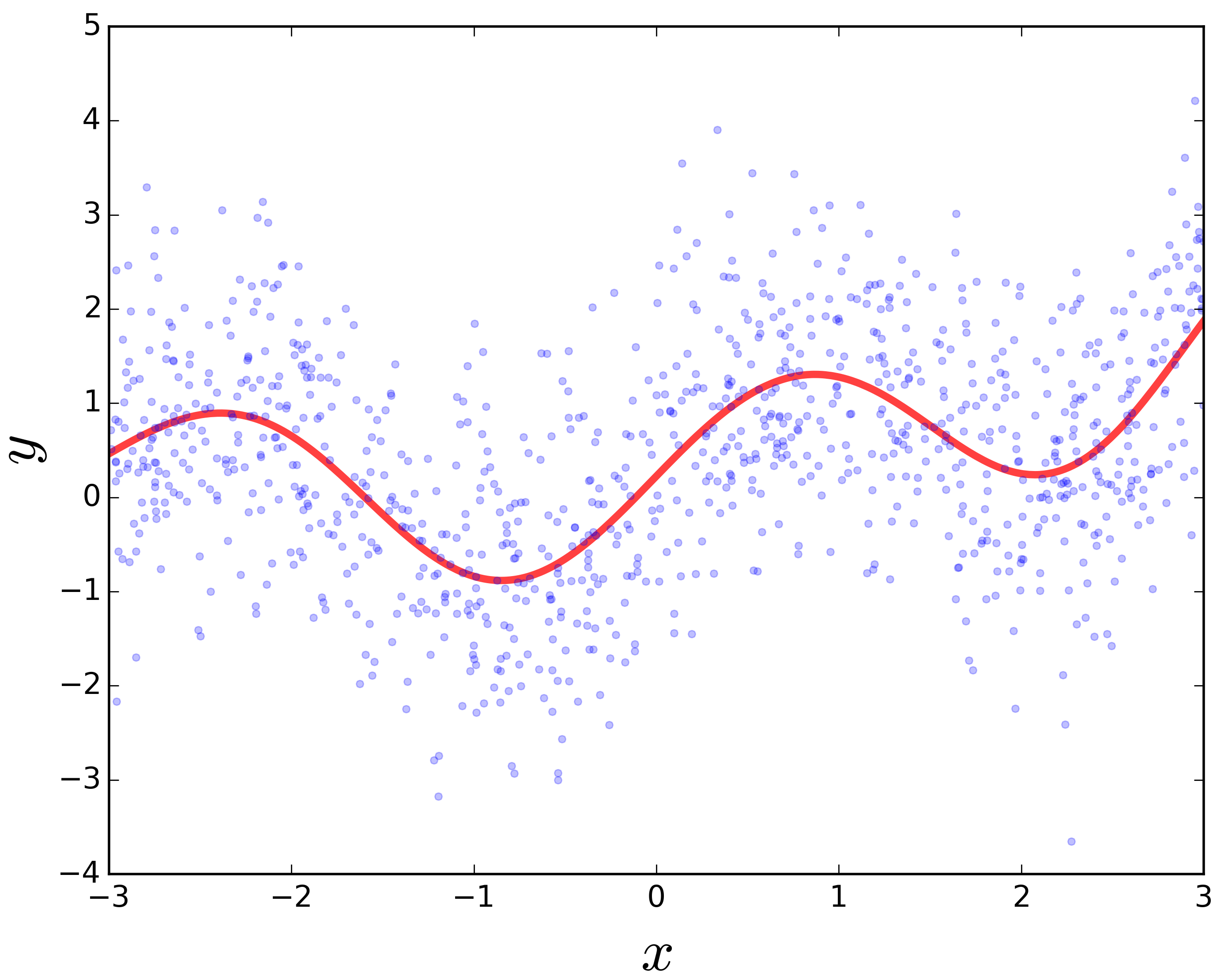
However, for varying values of , we present the difference between the for the exact (dense linear algebra) regression and the regression obtained using the matrix factorization algorithm of this paper. We generate data-points from the model:
| (33) |
where and is chosen randomly in the interval . The non-parametric regression curve (or estimate) under a Gaussian process prior (with zero mean) is then calculated at the same points as in (6) and (7):
| (34) |
where we have chosen our covariance kernel to be consistent with the previous numerical experiments:
| (35) |
No effort was made to adapt the covariance kernel to the synthetic data. For , the inferred curve through the data is shown in Figure 7. If dense linear algebra is used to invert to obtain the exact estimate , the for this data is:
| (36) | ||||
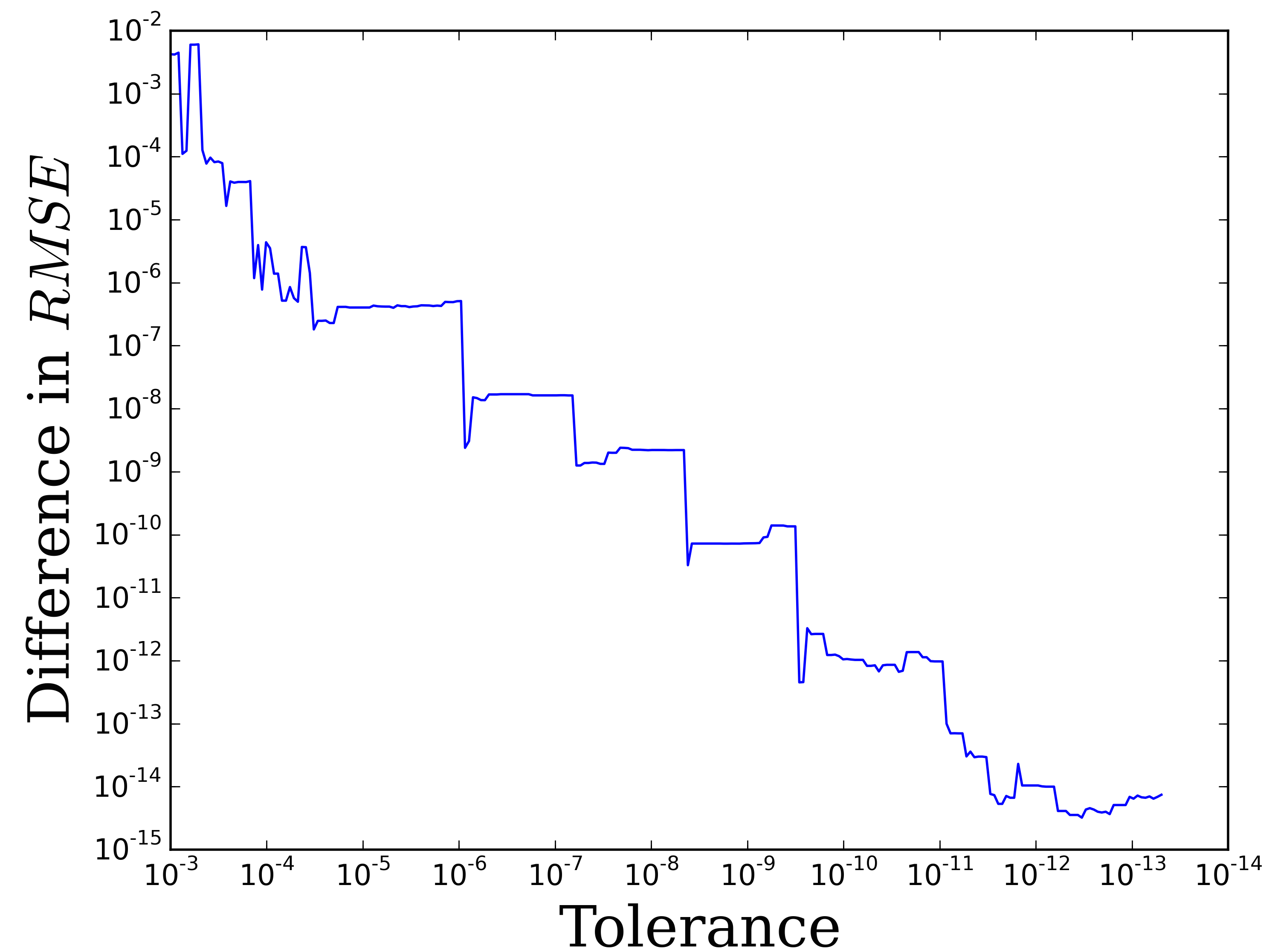
Figure 8 shows the absolute difference between the obtained from dense linear algebra and that obtained from our accelerated scheme as a function of factorization precision . Unsurprisingly, from this plot we determine that, indeed, the difference in regression performance (at least as measured by ) is proportional to .
VI Conclusions
In this paper, we have presented a fast, accurate, and nearly optimal hierarchical direct linear algebraic algorithms for computing determinants, inverses, and matrix-vector products involving covariances matrices encountered when using Gaussian processes. Similar matrices appear in problems of classification and prediction; our method carries over and applies equally well to these problems. Previous attempts at accelerating these calculations (inversion and determinant calculation) relied on either sacrificing fidelity in the covariance kernel (e.g. thresholding), constructing a global low-rank approximation to the covariance kernel, or paying the computational penalty of dealing with dense, full-rank covariance matrices. Our HODLR-based algorithm obviates the need for this compromise. Our observation that many covariance matrices of mathematical statistics have fine-grained, compressible hierarchical structure that provides access to the inverse may find use in many applications in the future.
The source code for the algorithm has been made available on GitHub. The HODLR package for solving linear systems and computing determinants is available at https://github.com/sivaramambikasaran/HODLR [3] and the Python Gaussian process package [22], george, has been made available at https://github.com/dfm/george. Both packages are open source, the HODLR package is released under the MPL2.0 license and george is released under the MIT license. Details on using these packages are available at their respective online repositories.
In its present form, our method degrades in performance when the -dimensional data has a covariance function based on points in with , as well as when the covariance function is oscillatory. Part of the performance loss cannot be avoided due to the curse of dimensionality. High-dimensional data is simply more complicated than low-dimensional data causing the off-diagonal blocks to have larger ranks (at least in the scenario of more and more data samples). The other part of the performance loss is in the compression. For high-dimensional data, analytic interpolatory low-rank approximations will provide faster and more robust approximations. Extensions of our approach to these cases is a subject of current research. We are also investigating high-dimensional anisotropic quadratures for marginalization and moment computation.
Acknowledgment
The authors would like to thank Iain Murray for several useful and detailed discussions.
References
- [1] A. G. Akritas, E. K. Akritas, and G. I. Malaschonok, “Various proofs of Sylvester’s (determinant) identity,” Math. Comput. Simulat., vol. 42, no. 4, pp. 585–593, 1996.
- [2] S. Ambikasaran, “Fast algorithms for dense numerical linear algebra and applications,” Ph.D. dissertation, Stanford University, 2013.
- [3] S. Ambikasaran, “A fast direct solver for dense linear systems,” https://github.com/sivaramambikasaran/HODLR, 2013.
- [4] S. Ambikasaran and E. Darve, “An Fast Direct Solver for Partial Hierarchically Semi-Separable Matrices,” J. Sci. Comput., vol. 57, no. 3, pp. 477–501, 2013.
- [5] S. Ambikasaran, J. Y. Li, P. K. Kitanidis, and E. Darve, “Large-scale stochastic linear inversion using hierarchical matrices,” Comput. Geosci., vol. 17, no. 6, pp. 913–927, 2013.
- [6] S. Ambikasaran, A. K. Saibaba, E. F. Darve, and P. K. Kitanidis, “Fast Algorithms for Bayesian Inversion,” in Computational Challenges in the Geosciences. Springer, 2013, pp. 101–142.
- [7] A. Aminfar, S. Ambikasaran, and E. Darve, “A fast block low-rank dense solver with applications to finite-element matrices,” arxiv.org/abs/1403.5337, 2014.
- [8] M. Anitescu, J. Chen, and L. Wang, “A Matrix-Free Approach for Solving the Parametric Gaussian Process Maximum Likelihood Problem,” SIAM J. Sci. Comput., vol. 34, pp. A240–A262, 2012.
- [9] R. P. Barry and R. K. Pace, “Monte Carlo estimates of the log determinant of large sparse matrices,” Lin. Alg. Appl., vol. 289, pp. 41–54, 1999.
- [10] S. Börm, L. Grasedyck, and W. Hackbusch, “Hierarchical matrices,” Lecture notes, vol. 21, 2003.
- [11] R. P. Brent, J.-A. H. Osborn, and W. D. Smith, “Bounds on determinants of perturbed diagonal matrices,” arxiv.org/abs/1401.7084, 2013.
- [12] O. Cappé, E. Moulines, and T. Rydén, Inference in hidden Markov models. New York, NY: Springer-Verlag, 2005.
- [13] K. Chalupka, C. K. I. Williams, and I. Murray, “A Framework for Evaluating Approximation Methods for Gaussian Process Regression,” J. Mach. Learn. Res., vol. 14, pp. 333–350, 2013.
- [14] S. Chandrasekaran, P. Dewilde, M. Gu, W. Lyons, and T. Pals, “A fast solver for HSS representations via sparse matrices,” SIAM J. Matrix Anal. Appl., vol. 29, no. 1, pp. 67–81, 2006.
- [15] S. Chandrasekaran, M. Gu, and T. Pals, “A fast ULV decomposition solver for hierarchically semiseparable representations,” SIAM J. Matrix Analysis and Applications, vol. 28, no. 3, pp. 603–622, 2006.
- [16] C. Chatfield, The Analysis of Time Series: An Introduction, 6th ed. Boca Raton, FL: Chapman and Hall, 2003.
- [17] J. Chen, L. Wang, and M. Anitescu, “A Fast Summation Tree Code for Matérn Kernel,” SIAM J. Sci. Comput., vol. 36, pp. A289–A309, 2013.
- [18] C. Dietrich and G. Newsam, “Fast and exact simulation of stationary gaussian processes through circulant embedding of the covariance matrix,” SIAM J. Sci. Comput., vol. 18, p. 1088, 1997.
- [19] A. Dutt and V. Rokhlin, “Fast Fourier Transforms for Nonequispaced Data,” SIAM J. Sci. Comput., vol. 14, no. 6, pp. 1368–1393, 1993.
- [20] ——, “Fast Fourier Transforms for Nonequispaced Data, II,” Appl. Comput. Harm. Anal., vol. 2, no. 1, pp. 85–100, 1995.
- [21] W. Fong and E. Darve, “The black-box fast multipole method,” J. Comput. Phys., vol. 228, no. 23, pp. 8712–8725, 2009.
- [22] D. Foreman-Mackey, “Fast Gaussian Processes for regression,” https://github.com/dfm/george, 2014.
- [23] A. Frieze, R. Kannan, and S. Vempala, “Fast Monte-Carlo algorithms for finding low-rank approximations,” J. ACM, vol. 51, no. 6, pp. 1025–1041, 2004.
- [24] Z. Gimbutas and V. Rokhlin, “A generalized fast multipole method for nonoscillatory kernels,” SIAM J. Sci. Comput., vol. 24, no. 3, pp. 796–817, 2003.
- [25] G. Golub and C. Van Loan, Matrix Computations. Johns Hopkins Univ Press, 1996, vol. 3.
- [26] S. Goreinov, E. Tyrtyshnikov, and N. Zamarashkin, “A theory of pseudoskeleton approximations,” Lin. Alg. Appl., vol. 261, no. 1-3, pp. 1–21, 1997.
- [27] L. Grasedyck and W. Hackbusch, “Construction and arithmetics of -matrices,” Computing, vol. 70, no. 4, pp. 295–334, 2003.
- [28] L. Greengard and J.-Y. Lee, “Accelerating the Nonuniform Fast Fourier Transform,” SIAM Rev., vol. 46, pp. 443–454, 2004.
- [29] L. Greengard and J. Strain, “The Fast Gauss Transform,” SIAM J. Sci. Stat. Comput., vol. 12, pp. 79–94, 1991.
- [30] L. Greengard, D. Gueyffier, P.-G. Martinsson, and V. Rokhlin, “Fast direct solvers for integral equations in complex three-dimensional domains,” Acta Numerica, vol. 18, no. 1, pp. 243–275, 2009.
- [31] L. Greengard and V. Rokhlin, “A fast algorithm for particle simulations,” J. Comput. Phys., vol. 73, no. 2, pp. 325–348, 1987.
- [32] M. Gu and S. Eisenstat, “Efficient algorithms for computing a strong rank-revealing QR factorization,” SIAM J. Sci. Comput., vol. 17, no. 4, pp. 848–869, 1996.
- [33] W. Hackbusch and S. Börm, “Data-sparse approximation by adaptive -matrices,” Computing, vol. 69, no. 1, pp. 1–35, 2002.
- [34] W. Hackbusch, “A Sparse Matrix Arithmetic Based on -Matrices. Part I: Introduction to -Matrices,” Computing, vol. 62, no. 2, pp. 89–108, 1999.
- [35] W. Hackbusch and B. N. Khoromskij, “A sparse -matrix arithmetic,” Computing, vol. 64, no. 1, pp. 21–47, 2000.
- [36] W. Hager, “Updating the inverse of a matrix,” SIAM Rev., pp. 221–239, 1989.
- [37] J. Hartikainen and S. Särkkä, “Kalman Filtering and Smoothing Solutions to Temporal Gaussian Process Regression Models,” in Proc. IEEE Int. Work. Mach. Learn. Signal Process., 2010.
- [38] J. Hensman, N. Fusi, and N. D. Lawrence, “Gaussian Processes for Big Data,” in Proc. 29th Conf. Uncertainty in Artificial Intelligence, A. Nicholson and P. Smyth, Eds. Corvallis, OR: AUAI Press, 2013, pp. 282–290.
- [39] K. L. Ho and L. Greengard, “A fast direct solver for structured linear systems by recursive skeletonization,” SIAM J. Sci. Comput., vol. 34, no. 5, pp. 2507–2532, 2012.
- [40] J. Y. Li, S. Ambikasaran, E. Darve, and P. K. Kitandis, “A Kalman filter powered by -matrices for quasi-continuous data assimilation problems,” Water Resour. Res., vol. 50, pp. 3734–3749, 2014.
- [41] E. Liberty, F. Woolfe, P.-G. Martinsson, V. Rokhlin, and M. Tygert, “Randomized algorithms for the low-rank approximation of matrices,” Proc. Natl. Acad. Sci. USA, vol. 104, no. 51, p. 20167, 2007.
- [42] D. J. MacKay, “Introduction to Gaussian processes,” NATO ASI Series F Computer and Systems Sciences, vol. 168, pp. 133–166, 1998.
- [43] P.-G. Martinsson and V. Rokhlin, “A fast direct solver for boundary integral equations in two dimensions,” J. Comput. Phys., vol. 205, no. 1, pp. 1–23, 2005.
- [44] L. Miranian and M. Gu, “Strong rank revealing LU factorizations,” Lin. Alg. Appl., vol. 367, pp. 1–16, 2003.
- [45] J. Q. nonero Candela and C. E. Rasmussen, “A unifying view of sparse approximate gaussian process regression,” J. Mach. Learn. Res., vol. 6, pp. 1939–1959, 2005.
- [46] F. W. J. Olver, D. W. Lozier, R. F. Boisvert, and C. W. Clark, Eds., NIST Handbook of Mathematical Functions. New York, NY: Cambridge University Press, 2010.
- [47] R. K. Pace and J. P. LeSage, “Chebyshev approximation of log-determinants of spatial weight matrices,” Comput. Stat. & Data Anal., vol. 45, pp. 179–196, 2004.
- [48] C.-T. Pan, “On the existence and computation of rank-revealing LU factorizations,” Lin. Alg. Appl., vol. 316, no. 1, pp. 199–222, 2000.
- [49] C. E. Rasmussen and C. Williams, Gaussian processes for machine learning. MIT Press, 2006.
- [50] S. Rjasanow, “Adaptive cross approximation of dense matrices,” IABEM 2002, International Association for Boundary Element Methods, 2002.
- [51] S. Särkkä, A. Solin, and J. Hartikainen, “Spatio-Temporal Learning via Infinite-Dimensional Bayesian Filtering and Smoothing,” IEEE Signal Process. Mag., vol. 30, no. 4, pp. 51–61, 2013.
- [52] Y. Shen, A. Ng, and M. Seeger, “Fast Gaussian process regression using KD-trees,” in Advances in Neural Information Processing Systems 18, Y. Weiss, Schölkopf, and J. Platt, Eds. MIT Press, Cambridge, MA, 2006, pp. 1225–1232.
- [53] J. Sherman and W. J. Morrison, “Adjustment of an inverse matrix corresponding to a change in one element of a given matrix,” Ann. Math. Stat., pp. 124–127, 1950.
- [54] A. J. Smola and P. L. Bartlett, “Sparse greedy gaussian process regression,” in Advances in Neural Information Processing Systems 13, T. K. Leen, T. G. Dietterich, and V. Tresp, Eds. MIT Press, Cambridge, MA, 2001, pp. 619–625.
- [55] E. Snelson and Z. Ghahramani, “Local and global sparse gaussian process approximations,” in Artifical Intelligence and Statistics (AISTATS 11), M. Meila and X. Shen, Eds., vol. 11, 2007, pp. 524–531.
- [56] E. L. Snelson, “Flexible and efficient gaussian process models for machine learning,” Ph.D. dissertation, Gatsby Computational Neuroscience Unit, University College London, 2007.
- [57] A. Solin and S. Särkkä, “Infinite-Dimensional Bayesian Filtering for Detection of Quasi-Periodic Phenomena in Spatio-Temporal Data,” Phys. Rev. E, vol. 88, no. 5, p. 052909, 2013.
- [58] A. Townsend and L. N. Trefethen, “Continuous analogues of matrix factorizations,” Proc. Roy. Soc. A, vol. 471, p. 20140585, 2015.
- [59] L. N. Trefethen, Approximation theory and approximation practice. Philadelphia, PA: SIAM, 2013.
- [60] G. N. Watson, A Treatise on the Theory of Bessel Functions. New York, NY: Cambridge University Press, 1995.
- [61] M. A. Woodbury, “Inverting modified matrices,” 1950, statistical Research Group, Memo. Rep. no. 42, Princeton University.
- [62] F. Woolfe, E. Liberty, V. Rokhlin, and M. Tygert, “A fast randomized algorithm for the approximation of matrices,” Appl. Comput. Harm. Anal., vol. 25, no. 3, pp. 335–366, 2008.
- [63] C. Yang, R. Duraiswami, and L. Davis, “Efficient kernel machines using the improved fast gauss transform,” in Advances in Neural Information Processing Systems 17, L. K. Saul, Y. Weiss, and L. Bottou, Eds. MIT Press, Cambridge, MA, 2005, pp. 1561–1568.
- [64] L. Ying, G. Biros, and D. Zorin, “A kernel-independent adaptive fast multipole algorithm in two and three dimensions,” J. Comput. Phys., vol. 196, no. 2, pp. 591–626, 2004.
- [65] L. Ying, “Fast algorithms for boundary integral equations,” in Multiscale Modeling and Simulation in Science. Springer, 2009, pp. 139–193.
- [66] K. Zhao, M. N. Vouvakis, and J.-F. Lee, “The Adaptive Cross Approximation Algorithm for Accelerated Method of Moments Computations of EMC Problems,” IEEE Trans. Electromagn. Compat., vol. 47, no. 4, pp. 763–773, 2005.
| Sivaram Ambikasaran obtained his Bachelor’s and Master’s in Aerospace Engineering from Indian Institute of Technology Madras in . Thereafter, he received his Master’s in Statistics, Master’s & Ph.D. in Computational Mathematics from Stanford University in , where he worked on fast direct solvers for large dense matrices. He is now a Courant Instructor at New York University. His research focuses on designing efficient, fast, scalable algorithms for mathematical problems arising out of physical applications. |
| Daniel Foreman-Mackey is a Ph.D. candidate in the Physics department at New York University. He received a B.Sc. from McGill University in 2008 and a M.Sc. in physics from Queen’s University (Canada) in 2010. His research is focused on comprehensive probabilistic data analysis projects in astrophysics, and specifically the field of exoplanets. |
| Leslie Greengard received a B.A. degree in Mathematics from Wesleyan University in 1979, a Ph.D. degree in Computer Science from Yale University in 1987, and an M.D. degree from Yale University in 1987. From 1987-1989 he was an NSF Postdoctoral Fellow at Yale University and at the Courant Institute of Mathematical Sciences, NYU, where he has been a faculty member since 1989. He was the Director of the Courant Institute from 2006-2011 and is presently Director of the Simons Center for Data Analysis at the Simons Foundation. His research interests include fast algorithms, acoustics, electromagnetics, elasticity, heat transfer, fluid dynamics, computational biology and medical imaging. Prof. Greengard is a member of the National Academy of Sciences and the National Academy of Engineering. |
| David W. Hogg obtained an S.B. from the Massachusetts Institute of Technology and a PhD in physics from the California Institute of Technology. His research has touched on large-scale structure in the Universe, the structure and formation of the Milky Way and other galaxies, and extra-solar planets. He currently works on engineering and data analysis aspects of large astronomical projects, with the goal of increasing discovery space and improving the precision and efficiency of astronomical measurements. |
| Michael O’Neil received an A.B. in Mathematics from Cornell University in 2003, and a Ph.D. in Applied Mathematics from Yale University in 2007 where he developed the generalized framework for butterfly-type algorithms, widely applicable to oscillatory integral operators. He was a postdoctoral fellow at the Courant Institute of Mathematical Sciences, NYU from 2010-2014. Presently, he is Assistant Professor of Mathematics at the Courant Institute, NYU and the Polytechnic School of Engineering, NYU. His research focuses on problems in computational electromagnetics, acoustics, and magnetohydrodynamics, integral equations, fast analysis-based algorithms, and computational statistics. |