Outlier eigenvalues for deformed i.i.d. random matrices

Abstract

We consider a square random matrix of size $N$ of the form $A+Y$ where $A$ is deterministic and $Y$ has iid entries with variance $1/N$. Under mild assumptions, as $N$ grows, the empirical distribution of the eigenvalues of $A+Y$ converges weakly to a limit probability measure $\beta$ on the complex plane. This work is devoted to the study of the outlier eigenvalues, i.e. eigenvalues in the complement of the support of $\beta$. Even in the simplest cases, a variety of interesting phenomena can occur. As in earlier works, we give a sufficient condition to guarantee that outliers are stable and provide examples where their fluctuations vary with the particular distribution of the entries of $Y$ or the Jordan decomposition of $A$. We also exhibit concrete examples where the outlier eigenvalues converge in distribution to the zeros of a Gaussian analytic function.

1 Introduction

1.1 Numerical instability of eigenvalues

The instability of the eigenvalues of badly conditioned matrices has dramatic consequences in the numerical computation of eigenvalues. As an example, take $N\geq 1$ be an integer and consider the standard nilpotent matrix

$$A_{N}=\sum_{i=1}^{N-1}e_{i+1}e_{i}^{*}=\begin{pmatrix}0&1&0&\cdots&0\\ 0&0&1&\cdots&0\\ \vdots&\vdots&\ddots&\ddots&\vdots\end{pmatrix}.$$ (1.1)

Its eigenvalues are obviously all zero. Let $U_{N}$ be a Haar-distributed orthogonal matrix and consider the unitarily equivalent matrix $B_{N}=U_{N}A_{N}U_{N}^{*}$. If we ask a computer to compute the eigenvalues of $B_{N}$, we obtain a surprising answer. Figure 1.1 is a plot of these numerically computed eigenvalues of $B_{N}$.

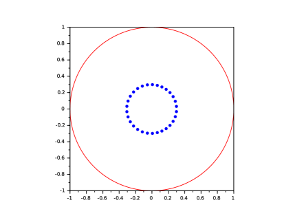
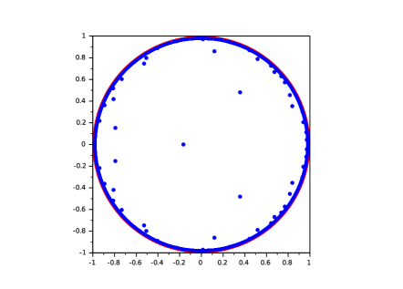
Figure 1.1: The blue dots are the numerically computed eigenvalues of $B_{N}=U_{N}A_{N}U_{N}^{*}$, the nilpotent matrix (1.1) conjugated by a Haar-distributed orthogonal matrix $U_{N}$ for $N=30$ and $N=2000$.

In the spirit of von Neumann and Goldstine [57], Spielman and Teng [52] or Edelman and Rao [27], a possible way to try to explain this phenomenon is to approximate numerical rounding errors by randomness and study the spectrum of the matrix

$$A_{N}+\sigma Y_{N},$$

where $Y_{N}$ is a random matrix normalized to have an operator norm of order $1$ and $\sigma$ is small positive parameter. As we shall see, in Subsection 1.5, in the limit $N\to\infty$ and then $\sigma\to 0$, one obtain a reasonable explanation of the right picture of Figure 1.1. A phenomenon related to the left figure, namely that the numerically estimated eigenvalues of a Jordan block are close to be roots of a small complex number will also be illustrated in Subsection 1.4

1.2 Deformed random matrices

For any $N\times N$ matrix $A$, denote by $\lambda_{1}(A),\ldots,\lambda_{N}(A)$ the eigenvalues of $A$ and by $\mu_{A}$ the empirical spectral measure of $A$:

$$\mu_{A}:=\frac{1}{N}\sum_{i=1}^{N}\delta_{\lambda_{i}(A)}.$$

We will consider the deformed model:

$$M_{N}=A_{N}+\sigma Y_{N},$$ (1.2)

where $\sigma>0$, $Y_{N}$ is a $N\times N$ random matrix and $A_{N}$ is a $N\times N$ deterministic matrix. The matrix $M_{N}$ can be thought as a random perturbation of the matrix $A_{N}$. Throughout this paper, we set

$$Y_{N}=\frac{X_{N}}{\sqrt{N}},$$ (1.3)

and we shall consider the following set of statistical assumptions on the matrices $X_{N}=(X_{ij})_{1\leq i,j\leq N}$:

1. $(X_{ij})_{i,j\geq 1}$ are independent and identically distributed complex random variables with $\mathbb{E}X_{ij}=0$, $\mathbb{E}|X_{ij}|^{2}=1$.

2. $\mathbb{E}|X_{ij}|^{4}<\infty$.

3. There exists $c>0$ such that for all $k\geq 1$ integer $\mathbb{E}|X_{ij}|^{k}\leq(ck)^{c}$.

Our first assumptions on the matrices $A_{N}$ are as follows:

1. There exists $M>0$ such that for all $N$, $\|A_{N}\|\leq M$.

2. For all $z\in\mathbb{C}$, $\mu_{(A_{N}-zI_{N})(A_{N}-zI_{N})^{*}}$ converges weakly to a probability measure $\nu_{z}$.

We start by recalling a generalization of the circular law to the deformed matrix model $M_{N}$.

Theorem 1.1.

Under assumptions (X1) and (A1-A2), there exists a deterministic probability measure $\beta$ on $\mathbb{C}$ such that, almost surely, $\mu_{M_{N}}$ converges weakly to $\beta$. Moreover, for any $z\in\mathbb{C}$, there exists a deterministic probability measure $\mu_{z}$ on $\mathbb{R}_{+}$ such that, almost surely, $\mu_{(M_{N}-zI_{N})(M_{N}-zI_{N})^{*}}$ converges weakly to $\mu_{z}$.

The first statement was first proved in Tao and Vu [55], the second statement was an ingredient of the proof, it is due to Dozier and Silverstein [25]. For more references, we refer to the surveys [54, 17]. In subsection 2.2, we will give a precise characterization of $\beta$ and $\mu_{z}$ in terms of $\sigma$ and $\nu_{z}$. The assumption (A1) can be weakened, see [15]. If $A_{N}=0$ then $\beta$ is the uniform distribution on $B(0,\sigma)$, the closed ball of radius $\sigma$ and center $0$ in $\mathbb{C}$. Beware that (i) assumptions (A1-A2) do not imply that $\mu_{A_{N}}$ converges weakly to a measure $\alpha$ on $\mathbb{C}$ (neither the opposite) and (ii) even though, it is not always the case that as $\sigma$ goes to $0$, $\beta$ converges weakly to $\alpha$.

We have not been able to compute the support of $\beta$ in general. There is however a typical situation where it takes a nice form. Observe first that $\lambda$ is an eigenvalue of $A_{N}$ if and only if $0$ is an eigenvalue of $(A_{N}-\lambda I_{N})(A_{N}-\lambda I_{N})^{*}$. We will assume that a similar property holds for $\beta$ and $\mu_{z}$, i.e.

1. $\mathrm{supp}(\beta)=\{z\in\mathbb{C}:0\in\mathrm{supp}(\mu_{z})\}$.

We are not aware of an example where (A3) fails to hold. We shall prove that (A3) holds if $\nu_{z}$ is the law of $|L-z|^{2}$ where $L$ is a random variable on $\mathbb{C}$ with distribution $\alpha$, (see the forthcoming Lemma 2.5). This case will occur if $A_{N}$ is a normal matrix and $\mu_{A_{N}}$ converges weakly to $\alpha$ (or if, for some normal matrix $B_{N}$, either $A_{N}-B_{N}$ has rank $o(N)$ or ${\rm Tr}(A_{N}-B_{N})(A_{N}-B_{N})^{*}=o(N)$). Under assumption (A3) the support of $\beta$ takes a particularly simple expression. We introduce

$$S=\{z\in\mathbb{C}:0\in\mathrm{supp}(\nu_{z})\}.$$

Proposition 1.2.

Suppose that assumptions (X1) and (A1-A3) hold. Then

$$\mathrm{supp}(\beta)=\left\{z\in\mathbb{C}:z\in S\hbox{ or }\int\lambda^{-1}d\nu_{z}(\lambda)\geq\sigma^{-2}\right\}.$$ (1.4)

For example, if $A_{N}=0$, then $\nu_{z}$ is a Dirac mass at $|z|^{2}$ and we retrieve the support of the circular law. If $A_{N}$ is given by (1.1), then $\nu_{z}$ is the law of $|L-z|^{2}$ with $L$ uniformly distributed on the unit complex circle. We find that $\mathrm{supp}(\beta)$ is the annulus with inner radius $\sqrt{(1-\sigma^{2})_{+}}$ and outer radius $\sqrt{1+\sigma^{2}}$. In the limit $\sigma\to 0$, $\mathrm{supp}(\beta)$ converges to the unit complex circle. This is consistent with Figure 1.1.

1.3 Stable outliers

We are now interested by describing the individual eigenvalues of $M_{N}$ outside $B(\mathrm{supp}(\beta),\varepsilon)$ for some $\varepsilon>0$. To this end, we shall fix a set $\Gamma\subset\mathbb{C}$ and assume that all but $O(1)$ of the eigenvalues of the matrix $A_{N}$ are outside $\Gamma$. To this end, we write

$$A_{N}=A^{\prime}_{N}+A^{\prime\prime}_{N}.$$

We first extend assumption (A1) to both $A^{\prime}_{N}$ and $A^{\prime\prime}_{N}$:

1. There exists $M>0$ such that for all $N$, $\|A^{\prime}_{N}\|+\|A^{\prime\prime}_{N}\|\leq M$.

Our next key assumption asserts that $A^{\prime}_{N}-zI_{N}$ is well conditioned in $\Gamma$ while $A^{\prime\prime}_{N}$ has small rank. We fix some integer $r\geq 0$.

1. $A^{\prime\prime}_{N}$ has rank $r$, and for any $z\in\Gamma ŝ$, there exists $\eta=\eta_{z}>0$ such that for all $N$ large enough, $(A^{\prime}_{N}-zI_{N})$ has no singular value in $[0,\eta]$.

When $\Gamma$ is compact, observe that (A4) implies that for some $\varepsilon>0$, the eigenvalues of $A^{\prime}_{N}$ are in $\mathbb{C}\backslash B(\Gamma,\varepsilon)$ for all $N$ large enough. In the case where $A^{\prime}_{N}$ is a normal matrix then the singular values of $(A^{\prime}_{N}-zI_{N})$ are $|\lambda_{k}(A^{\prime}_{N})-z|,1\leq k\leq N$. Hence, the assumption (A4) for $A^{\prime}_{N}$ normal and $\Gamma$ compact holds if and only if for some $\varepsilon>0$ and all $N$ large enough, the eigenvalues of $A^{\prime}_{N}$ lie in $\mathbb{C}\backslash B(\Gamma,\varepsilon)$.

Our first main result gives a sufficient condition to guarantee that outliers are stable.

Theorem 1.3.

Suppose that assumptions (X1-X2) and assumptions (A1’-A4) hold for $\Gamma\subset\mathbb{C}\backslash\mathrm{supp}(\beta)$ a compact set with continuous boundary. If for some $\varepsilon>0$ and all $N$ large enough,

$$\min_{z\in\partial\Gamma}\left|\frac{\det(A_{N}-z)}{\det(A^{\prime}_{N}-z)}\right|\geq\varepsilon,$$ (1.5)

then a.s. for all $N$ large enough, the number of eigenvalues of $A_{N}$ and $M_{N}$ in $\Gamma$ is equal.

Above, the notation (A1’-A4) stands for (A1’)-(A2)-(A3)-(A4). We will first prove Theorem 1.3 in the case $r=0$.

Theorem 1.4.

Suppose that assumptions (X1-X2) and assumptions (A1-A4) hold with $A^{\prime\prime}_{N}=0$, $A_{N}=A^{\prime}_{N}$ and $\Gamma\subset\mathbb{C}\backslash\mathrm{supp}(\beta)$ a compact set. Then, a.s. for all $N$ large enough, $M_{N}$ has no eigenvalue in $\Gamma$.

In particular, if (A4) holds with $r=0$ and $\Gamma=\mathbb{C}\backslash\mathrm{supp}(\beta)$ then for any $\varepsilon>0$, a.s. for all $N$ large enough, all eigenvalues of $M_{N}$ are in $B(\mathrm{supp}(\beta),\varepsilon)$.

Let us give a concrete application of Theorem 1.3 with a specific decomposition of $A_{N}=A^{\prime}_{N}+A^{\prime\prime}_{N}$. Assume that for all $N$, there exists a subset $J\subset\{1,\cdots,N\}$ of cardinal at most $r$ such that for any $\varepsilon>0$, for all $N$ large enough and $k\in J$, $\lambda_{k}(A_{N})\notin B(\mathrm{supp}(\beta),\varepsilon)$. We consider a triangular decomposition of $A_{N}$:

$$A_{N}=P\left(\begin{array}[]{c|c}T^{\prime\prime}&*\\ \hline\cr 0&T^{\prime}\end{array}\right)P^{-1},$$

where $P$ is an invertible matrix, $T^{\prime}$ is an upper triangular matrix of size $N-|J|$ with the eigenvalues $\lambda_{k}(A_{N})$, $k\notin J$, on the diagonal, and $T^{\prime\prime}$ is an upper triangular matrix of size $|J|$ with diagonal entries $\lambda_{k}(A_{N})$, $k\in J$. Fix some $a\in\mathrm{supp}(\beta)$, we decompose $A_{N}$ as $A_{N}=A^{\prime}_{N}+A^{\prime\prime}_{N}$ with

$$A^{\prime}_{N}=P\left(\begin{array}[]{c|c}aI_{J}&*\\ \hline\cr 0&T^{\prime}\end{array}\right)P^{-1}\quad\hbox{ and }\quad A^{\prime\prime}_{N}=P\left(\begin{array}[]{c|c}T^{\prime\prime}-aI_{J}&0\\ \hline\cr 0&0\end{array}\right)P^{-1}.$$ (1.6)

In particular,

$$\frac{\det(A_{N}-z)}{\det(A^{\prime}_{N}-z)}=\prod_{k\in J}\frac{\lambda_{k}(A_{N})-z}{a-z}.$$ (1.7)

The next statement will be an easy consequence of Theorem 1.3. It generalizes Tao [53, Theorem 1.7] where $A^{\prime}_{N}=0$. When $A^{\prime}_{N}$ is a Wigner random matrix, it is a special case of O’Rourke and Renfrew [41, Theorem 2.4].

Corollary 1.5.

Assume that assumptions (X1-X2) and assumptions (A1’-A4) hold with $A^{\prime}_{N}$, $A^{\prime\prime}_{N}$ given by (1.6) and $\Gamma=\mathbb{C}\backslash\mathrm{supp}(\beta)$. Fix $\varepsilon>0$. Assume that for all $N$ large enough, $\forall k\in J$, $\lambda_{k}(A_{N})\notin B(\mathrm{supp}(\beta),3\varepsilon)$. Then, a.s. for all $N$ large enough, there are exactly $|J|$ eigenvalues of $M_{N}$ in $\mathbb{C}\backslash B(\mathrm{supp}(\beta),2\varepsilon)$. Moreover, if we index them by $\lambda_{k}(M_{N})$, $k\in J$, after labeling properly, a.s.

$$\max_{k\in J}|\lambda_{k}(M_{N})-\lambda_{k}(A_{N})|\to 0.$$

In Figure 1.2, we illustrate numerically Corollary 1.5 when

$$A_{N}=\left(\begin{array}[]{c|c}B&0\\ \hline\cr 0&C\end{array}\right)\quad\hbox{with }B\in M_{r}(\mathbb{C})\hbox{ and }C=\sum_{i=r+1}^{N-1}e_{i}e_{i+1}^{*}+e_{N}e_{r+1}^{*}.$$ (1.8)

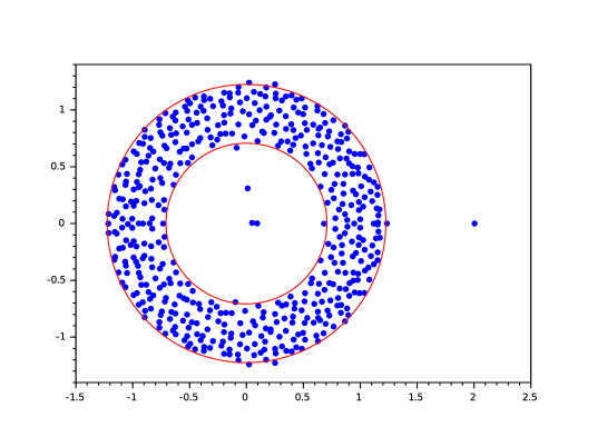
Figure 1.2: Eigenvalues of $M_{N}$ where $A_{N}$ is given by (1.8) with $r=5$ and $B$ has eigenvalues $(0,0,i/3,1,2)$, $N=500$, $\sigma^{2}=1/2$ and $X_{N}$ has real Gaussian entries. The support of $\beta$ is $\{z\in\mathbb{C}:1/\sqrt{2}\leq|z|\leq\sqrt{3/2}\}$, the stable outliers are $(0,0,i/3,2)$.

Assumption (1.5) is the key assumption for the stability of the outliers. It holds generically in the unbounded component of the complement of $S$.

Lemma 1.6.

Suppose that assumptions (A1’-A4) hold with $\Gamma=D$ an unbounded component of $\mathbb{C}\backslash S$. The family of $D\to\mathbb{C}$ functions $f_{N}:z\mapsto\det(A_{N}-z)/\det(A^{\prime}_{N}-z)$ is a precompact family of analytic functions and any subsequential limit of $(f_{N})$ is non-zero. In particular, along any converging subsequence $(f_{N_{k}})_{k\geq 1}$, for any $B(z,t)\subset D$ and any $\delta>0$, there exist $\varepsilon>0$ and $\Gamma=B(z,t^{\prime})$ with $t-\delta<t^{\prime}\leq t$ such that (1.5) holds for all $N_{k}$, $k\geq 1$.

In the sequel, in order to circumvent the multiple possible choices to order the eigenvalues, we will consider the finite point set $\sum_{i=1}^{n}\delta_{x_{i}}$ of a vector $(x_{1},\cdots,x_{n})$. Let us first recall some basic facts on finite point processes (we refer to Daley and Vere-Jones [23, Appendix A.2.5] for details and terminology). If $\mathcal{S}$ is a complete separable metric space, we denote by $\mathcal{N}(\mathcal{S})$, the set of finite point (integer valued) measures on $\mathcal{S}$, equipped with the usual weak topology. Recall that a point process is random variable on $\mathcal{N}(\mathcal{S})$. The set $\mathcal{P}(\mathcal{N}(\mathcal{S}))$ of probability measures on $\mathcal{N}(\mathcal{S})$ is a complete separable metric space and the Lévy-Prohorov distance is a metric for the weak convergence of measures in $\mathcal{P}(\mathcal{N}(\mathcal{S}))$ (or with a slight abuse of language, for weak convergence of point processes on $\mathcal{S}$).

1.4 Fluctuations of stable outliers

We have studied the fluctuations of the convergence of outliers eigenvalues in the simplest case for the decomposition of $A_{N}$ on its outlier eigenspace. More precisely, we will suppose that $A_{N}$ has the following decomposition, for some integer $r\geq 1$ and complex number $\theta_{N}$,

$$A_{N}=\left(\begin{array}[]{c|c}\theta_{N}I_{r}&0\\ \hline\cr 0&\hat{A}_{N-r}\end{array}\right).$$ (1.9)

Theorem 1.7.

Suppose that assumptions (X1-X2) and assumptions (A1-A3) hold with $A_{N}$ given by (1.9). We suppose further that $\theta_{N}$ converges toward $\theta\in\mathbb{C}\setminus\mathrm{supp}(\beta)$ when $N$ goes to infinity and that for some $\eta>0$ and all large $N$, $\hat{A}_{N-r}-\theta I_{N-r}$ has no singular value in $[0,\eta]$. Finally, assume that either $\mathbb{E}X_{11}^{2}=0$ or that $\frac{1}{N-r}{\rm Tr}\left\{(\theta I_{N-r}-\hat{A}_{N-r})^{-1}(\theta I_{N-r}-\hat{A}_{N-r}^{\top})^{-1}\right\}$ converges to $\psi\in\mathbb{C}$ (in the first case, we set $\psi=0$). We set $\varphi=\int\lambda^{-1}d\nu_{\theta}(\lambda)$.

Then, for any $0<\delta<\eta$, almost surely for all large $N$ there are exactly $r$ eigenvalues $\lambda_{i}$, $i=1,\ldots,r$ of $M_{N}$ in $B(\theta,\delta)$. Moreover, the point process of $\left(\sqrt{N}(\lambda_{1}-\theta_{N}),\ldots,\sqrt{N}(\lambda_{r}-\theta_{N})\right)$ converges in distribution towards the point process of the eigenvalues of a $r\times r$ matrix $V$ defined as

$$V=\sigma X_{r}+\sigma^{2}G,$$ (1.10)

where $X_{r}$ is independent of $G$, a $r\times r$ Ginibre matrix whose entries are independent copies of a centered complex Gaussian variable $Z$ whose covariance is characterized by,

$$\mathbb{E}|Z|^{2}=\frac{\varphi}{1-\sigma^{2}\varphi}\quad\hbox{ and }\quad\mathbb{E}Z^{2}=\frac{(\mathbb{E}X_{11}^{2})^{2}\psi}{1-\sigma^{2}\mathbb{E}X_{11}^{2}\psi}.$$

Theorem 1.7 shows that the fluctuation of stable outliers are not universal (they may depend on the law of entries). There is a similar phenomenon for deformed Wigner matrices, see notably Capitaine, Donati-Martin and Féral [20, 21]. The left plot of Figure 1.3 illustrates Theorem 1.7.

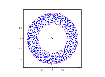
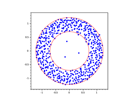
Figure 1.3: Eigenvalues of $M_{N}$ for $A_{N}$ given (1.8) with $\sigma^{2}=1/2$, $X_{N}$ has complex Gaussian entries, $N=500$ and $r=3$. On the left: $B=0$. On the right: $B=e_{1}e_{2}^{*}+e_{2}e_{3}^{*}$, we have $N^{1/(2r)}=N^{1/6}\simeq 0.35$ !

It was recently discovered by Benaych-Georges and Rochet [12] in the related study of the outliers in the single ring theorem (see discussion and related results below) that the fluctuations can be larger than $1/\sqrt{N}$ when the Jordan decomposition of an eigenvalue is not a diagonal matrix. Inspired by their work, we have also studied the fluctuations when for some integer $r\geq 2$ and complex number $\theta_{N}$,

$$A_{N}=\left(\begin{array}[]{c|c}\hat{A}_{r}&0\\ \hline\cr 0&\hat{A}_{N-r}\end{array}\right),\hbox{ with }\quad\quad\hat{A}_{r}=P_{N}J_{N}P_{N}^{-1},\quad P_{N}\in\mathrm{GL}_{r}(\mathbb{C}),$$ (1.11)

and $J_{N}\in M_{r}(\mathbb{C})$ is the Jordan matrix

$$J_{N}=\begin{pmatrix}\theta_{N}&1&&&\\ &\theta_{N}&1&&\\ &&\ddots&\ddots&\end{pmatrix}.$$

Theorem 1.8.

Suppose that assumptions (X1-X2) and assumptions (A1-A3) hold with $A_{N}$ given by (1.11). We suppose further that $\theta_{N}$ converges toward $\theta\in\mathbb{C}\setminus\mathrm{supp}(\beta)$ when $N$ goes to infinity and that for some $\eta>0$ and all large $N$, $\hat{A}_{N-r}-\theta I_{N-r}$ has no singular value in $[0,\eta]$. Assume finally that $\|P_{N}-P\|\to 0$ for some $P\in\mathrm{GL}_{r}(\mathbb{C})$, and that either $\mathbb{E}X_{11}^{2}=0$ or that $\frac{1}{N-r}{\rm Tr}\left\{(\theta I_{N-r}-\hat{A}_{N-r})^{-1}(\theta I_{N-r}-\hat{A}_{N-r}^{\top})^{-1}\right\}$ converges to $\psi\in\mathbb{C}$ (in the first case, we set $\psi=0$).

Then, for any $0<\delta<\eta$, almost surely for all large $N$ there are exactly $r$ eigenvalues $\lambda_{i}$, $i=1,\ldots,r$ of $M_{N}$ in $B(\theta,\delta)$. Moreover, the point process of $\left(N^{1/(2r)}(\lambda_{1}-\theta_{N}),\ldots,N^{1/(2r)}(\lambda_{r}-\theta_{N})\right)$ converges in distribution towards the point process of the roots of the random polynomial

$$z^{r}-e_{r}^{*}P^{-1}VPe_{1},$$

where $V$ is defined by (1.10).

When $\hat{A}_{N-r}=0$ and $X_{N}$ is a complex Ginibre matrix, the above result is contained in [12, Theorem 2.6]. This result shows the strong correlation of the outlier eigenvalues in the setting of Theorem 1.8: properly rescaled they are asymptotically the $r$-th roots of the same random complex number. The right plot of Figure 1.3 illustrates Theorem 1.8.

1.5 Unstable outliers

Lemma 1.6 does not rule out the possibility that (1.5) fails to hold in a bounded component of $\mathbb{C}\backslash S$. Let us give a typical situation where (1.5) does not hold. Consider the nilpotent matrix $A_{N}$ given by (1.1). We have $A_{N}=A^{\prime}_{N}+A^{\prime\prime}_{N}$ with

$$A^{\prime}_{N}=\sum_{i=1}^{N-1}e_{i}e_{i+1}^{*}+e_{N}e_{1}^{*}\quad\hbox{ and }\quad A^{\prime\prime}_{N}=-e_{N}e_{1}^{*}.$$

$A^{\prime}_{N}$ is a permutation matrix whose eigenvalues are for $1\leq\ell\leq N$, $\omega_{\ell}=e^{\frac{2i\pi\ell}{N}}$ with associated normalized eigenvector $f_{\ell}=(\omega_{\ell}^{k}/\sqrt{N})_{1\leq k\leq N}$. In particular, if $|z|\leq 1-\varepsilon$,

$$\left|\frac{\det(A_{N}-z)}{\det(A^{\prime}_{N}-z)}\right|=\frac{|z|^{N}}{|1-z^{N}|}\leq\frac{(1-\varepsilon)^{N}}{1-(1-\varepsilon)^{N}}$$

decreases exponentially fast. Hence Assumption (1.5) does not hold for $\Gamma\subset B(0,1-\varepsilon)$. In Figure 1.4, we see numerically that the conclusion of Theorem 1.3 does not seem to hold. Also, (1.1) can be interpreted as a limit case of (1.11) when $r=N$. Then, Theorem 1.8 hints at macroscopic fluctuations of outlier eigenvalues.

Figure 1.4: Eigenvalues of $M_{N}$ where $A_{N}$ given by (1.1) with $N=500$, $\sigma^{2}=1/2$ and $X_{N}$ has real Gaussian entries. There are outlier eigenvalues in the bounded component of the complement of $\mathrm{supp}(\beta)=\{z\in\mathbb{C}:1/\sqrt{2}\leq|z|\leq\sqrt{3/2}\}$.

To have a better picture, we may rewrite $A_{N}$ in the orthonormal basis of eigenvectors of $A^{\prime}_{N}$. We have $A^{\prime}_{N}=U_{N}B^{\prime}_{N}U_{N}^{*}$ with

$$B^{\prime}_{N}=\mathrm{diag}(\omega_{1},\cdots,\omega_{N})$$ (1.12)

and $A^{\prime\prime}_{N}=U_{N}B^{\prime\prime}_{N}U_{N}^{*}$ with

$$B^{\prime\prime}_{N}=-f_{N}f_{1}^{\top}.$$ (1.13)

Hence, an important difference with the setting of Theorem 1.7 is that $A^{\prime\prime}_{N}$ has a strongly delocalized decomposition in the orthonormal basis of eigenvectors of $A^{\prime}_{N}$. This motivates the results of this paragraph.

For simplicity, we will reinforce the assumption (A4) by assuming that $A^{\prime}_{N}$ is diagonal.

1. $A^{\prime\prime}_{N}$ has rank $r$, $A^{\prime}_{N}$ is diagonal and for some $\varepsilon>0$ and all $N$ large enough, all eigenvalues of $A^{\prime}_{N}$ lie in $\mathbb{C}\backslash B(\Gamma,\varepsilon)$.

If $A^{\prime}_{N}$ is a normal matrix and $X_{ij}$ are standard complex Gaussian variables, then, by unitary invariance, we can always assume that (A4’) holds if (A4) holds.

We endow the set of analytic functions on a bounded connected open subset $U$ of $\mathbb{C}$ with the distance

$$d(f,g)=\sum_{j\geq 1}2^{-j}\frac{\|f-g\|_{K_{j}}}{1+\|f-g\|_{K_{j}}},$$ (1.14)

where $(K_{j})_{j\geq 1}$ is an exhaustion by compact sets of $U$ and $\|f-g\|_{K_{j}}$ denotes the infinity norm of $f-g$ on $K_{j}$. We recall that it is complete separable metric space. The interior of a set $K$ is denoted by $\mathring{K}$.

Theorem 1.9.

Assume that assumptions (X1-X3) and assumptions (A1’-A4’) hold with $r=1$ and $\Gamma\subset\mathbb{C}\backslash\mathrm{supp}(\beta)$ a compact set with continuous boundary. Assume further that $A^{\prime\prime}_{N}=v_{N}u_{N}^{*}$ where $\|u_{N}\|_{\infty},\|v_{N}\|_{\infty}$ are of order $O(1/\sqrt{N})$ and

$$\max_{z\in\Gamma}\left|\frac{\det(A_{N}-z)}{\det(A^{\prime}_{N}-z)}\right|=o\left(\frac{1}{\sqrt{N}}\right).$$ (1.15)

Consider the centered Gaussian process $(g_{N}(z))_{z\in\Gamma}$ with covariance given by, for $z,w\in\Gamma$,

$$\mathbb{E}g_{N}(z)\bar{g}_{N}(w) = \frac{u_{N}^{*}R^{\prime}_{N}(z)(R^{\prime}_{N}(w))^{*}u_{N}v_{N}^{*}(R^{\prime}_{N}(w))^{*}R^{\prime}_{N}(z)v_{N}}{1-\sigma^{2}\varphi_{N}(z,w)}$$

$$\mathbb{E}g_{N}(z)g_{N}(w) = \frac{u_{N}^{*}R^{\prime}_{N}(z)R^{\prime}_{N}(w)\bar{u}_{N}v_{N}^{T}(R^{\prime}_{N}(w))^{T}R^{\prime}_{N}(z)v_{N}\mathbb{E}X_{11}^{2}}{1-\mathbb{E}X_{11}^{2}\sigma^{2}\psi_{N}(z,w)}$$

where $R^{\prime}_{N}(z)=(zI_{N}-A^{\prime}_{N})^{-1}$, $\varphi_{N}(z,w)=\frac{1}{N}{\rm Tr}R^{\prime}_{N}(z)(R^{\prime}_{N}(w))^{*}$ and $\psi_{N}(z,w)=\frac{1}{N}{\rm Tr}R^{\prime}_{N}(z)R^{\prime}_{N}(w)$.

Then, $g_{N}$ is a tight sequence of random analytic functions in $\mathring{\Gamma}$. Moreover, the Lévy-Prohorov distance between the point process of eigenvalues of $M_{N}$ in $\mathring{\Gamma}$ and the point process of zeros of $g_{N}$ in $\mathring{\Gamma}$ goes to $0$ as $N$ goes to $\infty$.

The intensity of zeros of $g_{N}$ can be computed explicitly thanks the Edelman-Kostlan’s formula, see [26, Theorem 3.1]. With the material of this paper, it is possible to generalize Theorem 1.9 for $r\geq 1$. The analog of condition (1.15) will however be more complicated and the analog of $g_{N}$ will be the determinant of $r\times r$ random Gaussian matrix (see forthcoming Remark 6.1).

In §6.5, we will give a general method to find perturbations $A^{\prime\prime}_{N}$ such that (1.15) holds. In the specific case of the nilpotent matrix (1.1), formulas are simpler. Following the terminology of Hough, Krishnapur, Peres, Virág [34], we say that $g$ is a Gaussian analytic function on a domain $\Gamma\subset\mathbb{C}$, if $g$ is a random analytic function on $\Gamma$, $(g(z),z\in\Gamma)$ is a Gaussian process and for $z,w\in\Gamma$, $\mathbb{E}g(z)g(w)=0.$

The next corollary deals with the phenomenon illustrated by Figure 1.4.

Corollary 1.10.

Let $A_{N}=B^{\prime}_{N}+B^{\prime\prime}_{N}$ with $B^{\prime}_{N}$ and $B^{\prime\prime}_{N}$ given by (1.12) and (1.13). Suppose that assumptions (X1-X3) hold. We set

$$\varphi(z,w)=\frac{1}{1-z\bar{w}}.$$ (1.16)

The support of $\beta$ is $\{z\in\mathbb{C}:\sqrt{(1-\sigma^{2})_{+}}\leq|z|\leq\sqrt{1+\sigma^{2}}\}$. If $\sigma<1$, the point process of eigenvalues of $M_{N}$ in $\mathring{B}(0,\sqrt{1-\sigma^{2}})$ converges weakly to the zeros of the Gaussian analytic function $g(z)$ on $\mathring{B}(0,\sqrt{1-\sigma^{2}})$ with kernel given by, for $z,w\in\Gamma$,

$$K(z,w)=\frac{\varphi(z,w)^{2}}{1-\sigma^{2}\varphi(z,w)}.$$

We may notice the following surprising fact. As $\sigma\to 0$, the kernel $K(z,w)$ appearing in Corollary 1.10 does not vanish, it converges pointwise to the kernel $K_{0}(z,w)=\varphi(z,w)^{2}$ on the unit complex disc. The kernel $K_{0}$ is the kernel of the Gaussian analytic function

$$g(z)=\sum_{k=0}^{\infty}z^{k}\gamma_{k}\sqrt{k+1},$$

where $\gamma_{k}$ are iid complex Gaussian variables with $\mathbb{E}\gamma_{k}^{2}=0$, $\mathbb{E}|\gamma_{k}|^{2}=1$. This Gaussian analytic function may thus be related to the numerical phenomenon illustrated by the right plot of Figure 1.1.

Finally, as in Rajan and Abbott [45] and Tao [53], interesting outliers may appear when $\|A^{\prime\prime}_{N}\|$ is of order $\sqrt{N}$.

Theorem 1.11.

Assume that assumptions (X1-X3) and assumptions (A2-A4’) hold with $r=1$ and $\Gamma\subset\mathbb{C}\backslash\mathrm{supp}(\beta)$ a compact set with continuous boundary. We set $R^{\prime}_{N}(z)=(zI_{N}-A^{\prime}_{N})^{-1}$, and assume further that $\|A^{\prime}_{N}\|=O(1)$ and $A^{\prime\prime}_{N}=\sqrt{N}v_{N}u_{N}^{*}$ where $\|u_{N}\|_{\infty},\|v_{N}\|_{\infty}$ and $u_{N}^{*}R^{\prime}_{N}(z)v_{N}$ are of order $O(1/\sqrt{N})$.

Consider the centered Gaussian process $(g_{N}(z))_{z\in\Gamma}$ of Theorem 1.9. Then, the Lévy-Prohorov distance between the point process of eigenvalues of $M_{N}$ in $\mathring{\Gamma}$ and the point process of zeros of $1-\sqrt{N}u_{N}^{*}R^{\prime}_{N}(z)v_{N}+\sigma g_{N}(z)$ in $\mathring{\Gamma}$ goes to $0$ as $N$ goes to $\infty$.

Figure 1.5: Eigenvalues of $M_{N}$ where $A_{N}=B^{\prime}_{N}-\sqrt{N}B^{\prime\prime}_{N}$ given by (1.12) and (1.13), $N=500$, $\sigma^{2}=1/2$ and $X_{N}$ has complex Gaussian entries. For $|z|>1$, we have $f_{N}^{T}R^{\prime}_{N}(z)f_{1}=1/(z^{N}-1)=o(1/\sqrt{N})$. The outlier eigenvalues in the unbounded component of the complement of $\mathrm{supp}(\beta)=\{z\in\mathbb{C}:1/\sqrt{2}\leq|z|\leq\sqrt{3/2}\}$ converge in distribution to the zeros of $1+\sigma g$ where $g$ is the Gaussian analytic function with kernel $H(z,w)=\varphi(z,w)^{2}/(1+\sigma^{2}\varphi(z,w))$ and $\varphi$ given by (1.16).

This result is illustrated with Figure 1.5. As an application, we have for example the following corollary which is related to [53, Theorem 1.11].

Corollary 1.12.

Assume that assumptions (X1-X3) hold, that $\sigma=1$, $A^{\prime}_{N}=0$ and $A_{N}=A^{\prime\prime}_{N}=\theta_{N}v_{N}u_{N}^{T}$ with $\sqrt{N}/\theta_{N}\to\kappa\in\mathbb{C}$, $u_{N},v_{N}\in\mathbb{R}^{N}$, $\|u_{N}\|=\|v_{N}\|=1$, $\theta_{N}u_{N}^{T}v_{N}\to\lambda\in\mathbb{C}$ and $\|u_{N}\|_{\infty},\|v_{N}\|_{\infty}$ are of order $O(1/\sqrt{N})$. Fix $\varepsilon>0$ and set $\Gamma=\mathbb{C}\backslash B(0,1+\varepsilon)$. We consider $g(z)=\sum_{k\geq 0}\gamma_{k}z^{-k}$ with $\gamma_{k}$ independent complex Gaussian variables with variance given by $\mathbb{E}|\gamma_{k}|^{2}=1$ and $\mathbb{E}\gamma_{k}^{2}=(\mathbb{E}X_{11}^{2})^{k+1}$.

Then, as $N$ goes to $\infty$, the point process of eigenvalues of $M_{N}$ in $\Gamma$ converges vaguely to the point process of zeros of $\kappa z(z-\lambda)+g(z)$ in $\Gamma$.

Observe that $\theta_{N}u_{N}^{T}v_{N}$ is the outlier eigenvalue of $A_{N}$. Hence, in the limit $|\kappa|\to\infty$, we find a result consistent with Theorem 1.3. Moreover, when $\mathbb{E}X_{11}^{2}=0$, $g(z)$ is a Gaussian analytic function, and, if $\kappa=0$, we are interested by the level set zero of this Gaussian analytic function. From Peres and Virág [43], it is known that this level set forms a determinantal point process.

1.6 Discussion and related results

In a recent work [12], Benaych-Georges and Rochet consider matrices of the type $M_{N}=X_{N}+A_{N}$ where the rank of $A_{N}$ stays bounded as the dimension goes to infinity and $X_{N}$ is a random non Hermitian matrix whose distribution is invariant under the left and right actions of the unitary group. The limiting empirical eigenvalues distribution of such a model is described by the so-called single ring theorem, see [31, 32, 49], and its support is of the form $\{z,a\leq|z|\leq b\}$. Benaych-Georges and Rochet prove that if $A_{N}$ has some eigenvalues out of the maximal circle of the single ring, then $M_{N}$ has outliers in the neighborhood of these eigenvalues of $A_{N}$. Nevertheless, when $a>0$, the eigenvalues of $A_{N}$ which may be in the inner disk of the complement of the limiting support do not generate outliers in the spectrum of $M_{N}$.

Now, in the framework of the present paper dealing with full rank perturbations of iid matrices, there can be outlier eigenvalues in bounded components of the complement of $\mathrm{supp}(\beta)$, see the example given by (1.8) and Figure 1.2.

Actually, the nature of the bounded connected component of the complement of the support of the limiting empirical eigenvalues distributions considering above is different: the first (in [12]) comes from the limiting support of the non-deformed model whereas the second one (in the framework of our paper) is created by the deformation. Subordination-like properties of the Stieltjes transform $g_{\mu}(z)=\int d\mu(\lambda)/(z-\lambda)$ of limiting spectral measures may help to understand these phenomena as explained below.

In the case of [12], since the limiting empirical eigenvalues distribution $\mu$ is radial, we have $g_{\mu}(z)=\frac{1}{z}$ if $|z|>b$ and $g_{\mu}(z)=0$ if $|z|<a$ so that roughly speaking

$$g_{\mu}(z)=g_{\delta_{0}}(\omega(z))~{}~{}\mbox{~{}~{}where~{}~{}}\left\{\begin{array}[]{ll}\omega(z)=z\mbox{~{}if~{}}|z|>b\\ \mbox{``}\omega(z)=\infty\mbox{"~{}if~{}}|z|<a.\end{array}\right.$$

In our case, dealing for instance with diagonal perturbations of a Ginibre matrix, the limiting empirical eigenvalues distribution $\beta$ is the Brown measure of $c+a$ where $c$ is a circular element which is free with $a$ whose Brown measure is $\alpha$ (see Śniady [51]). We have the following subordination property.

$$\forall z\in\mathbb{C}\setminus\mathrm{supp}(\beta),\;g_{c+a}(z)=g_{a}(\omega(z))\mbox{~{}~{}where~{}~{}}\omega(z)=z.$$

It can be deduced from [16, Proposition 4.3], see also [56, 13].

In both cases, the intuition is that

$$g_{\mu_{M_{N}}}(z)\approx g_{\mu_{A_{N}}}(\omega(z))$$

and that therefore they will be eigenvalues $\rho$ of $M_{N}$ that separate from the bulk whenever some of the equations $\omega(\rho)=\theta$ admits a solution $\rho$ outside the limiting support, when $\theta$ describes the spectrum of $A_{N}$.

Therefore, we understand in one hand that in the framework of [12], there is no solution inside the inner disk of such an equation since there $\omega\equiv\infty$ and in the other hand that the outliers of the deformed model stay in the neighborhood of the eigenvalues of the perturbation which are located where $\omega$ is the identity function.

In [28], Feldheim, Paquette and Zeitouni have recently studied the model (1.2) when $\sigma$ decays polynomially of $N$ and $A_{N}$ is a block diagonal matrix with blocks of size $\log N$.

Note that motivated by the seminal article of Baik, Ben Arous and Péché [6], previous works are devoted to the study of the outlier eigenvalues of deformed random Hermitian matrix models, see notably [7, 4, 8, 9, 10, 11, 18, 20, 21, 22, 29, 35, 36, 37, 38, 42, 44, 46, 47]. Actually, the papers [8, 18, 22] already show that the results on existence and location of outliers of deformed Wigner matrices/ deformed unitarily invariant matrices/ sample covariance matrices/ information-plus-noise type matrices can be completely described in terms of subordination functions involved in free additive/multiplicative/rectangular convolutions. Thus, free subordination properties definitely seem to provide a global explanation for the problem of existence and location of outliers of deformed random matrix models.

In the Hermitian deformed models, the outliers of the deformed model are not located in a neighborhood of the spikes of the deformation. It contrasts with Corollary 1.5. It is rather non-intuitive that additive perturbation of $A_{N}$ by a Hermitian random matrix has more effect on outlier eigenvalues than additive perturbation by a non-Hermitian random matrix.

The remainder of the papers is organized as follows. In Section 2, we review some properties of the limiting spectral measures $\beta$ and $\mu_{z}$ and recall basic matrix identities, we notably prove Proposition 1.2 and Lemma 1.6. In Section 3 and Section 4, we prove the first order results, Theorem 1.4 and Theorem 1.3 respectively. In Section 5, we prove the central limit theorem for stable outliers, Theorem 1.7. In Section 6, we prove all results concerning unstable outliers, Theorem 1.9, Corollary 1.10, Theorem 1.9 and Corollary 1.10. Finally, an appendix contains a central limit theorem for a random bilinear form.

2 Preliminaries on limiting spectral measures and useful matrix relations

2.1 Useful matrix identities and perturbation inequalities

If $A\in M_{N}(\mathbb{C})$ we will denote by $s_{N}(A)\leq\ldots\leq s_{1}(A)$ the singular values of $A$. We have $s_{1}(A)=\|A\|$ and $s_{N}(A)^{-1}=\|A^{-1}\|$ where $\|A\|$ denotes the operator norm. In this work, we will repeatedly use the following classical perturbation inequalities. If $A,B$ in $M_{n}(\mathbb{C})$ then

$$|s_{i}(A)-s_{i}(B)|\leq\|A-B\|.$$ (2.1)

It follows immediately from Courant-Fisher variational formulas for the singular values, see e.g. [2, Theorem A.46]. We will often apply it in the following context, if $A-zI_{N}$ has no singular value in the interval $[0,\eta]$ and $\|B\|\leq\eta/3$ then

$$\sup_{w:|z-w|\leq\eta/2}\|(A-wI_{N})^{-1}\|\leq 2\eta^{-1}\quad\hbox{ and }\quad\sup_{w:|z-w|\leq\eta/3}\|(A+B-wI_{N})^{-1}\|\leq 3\eta^{-1}.$$ (2.2)

Similarly, if $K\subset\mathbb{C}$ is compact and for all $z\in K$, there exists $\eta_{z}>0$ such that $A-zI_{N}$ has no singular value in $[0,\eta_{z}]$ then, there exists $C_{K}$ such that

$$\sup_{z\in K}\|(A-zI_{N})^{-1}\|\leq C_{K},$$ (2.3)

($K$ is covered by $\cup_{z\in K}B(z,\eta_{z}/2)$ and use compactness).

As in previous works such as [10, 11], we will use the identity, if $P,Q^{\top}\in M_{N,r}(\mathbb{C})$,

$$\det(I_{N}+PQ)=\det(I_{r}+QP).$$

It will imply notably that for any $M\in M_{N}(\mathbb{C})$ and $\lambda\in\mathbb{C}$ such that $M_{N}-\lambda I_{N}$ is invertible,

$$\det(\lambda I_{N}-M-PQ)=\det(\lambda I_{N}-M)\det(I_{r}-Q(\lambda I_{N}-M)^{-1}P).$$ (2.4)

In particular the eigenvalues of $M+PQ$ which are not eigenvalues of $M$ are the zeros of an $r\times r$ determinant. With $M=A^{\prime}_{N}+\sigma Y_{N}$ and $PQ=A^{\prime\prime}_{N}$, the above identity will be our starting point to study the outlier eigenvalues.

2.2 Characterization of the limit measure $\beta$

For a probability measure $\tau$ on $\mathbb{C}$ such that $\int\log(1+|\lambda|)d\tau(\lambda)<\infty$, we denote by $h_{\tau}$ its logarithmic potential defined for $z\in\mathbb{C}$, by

$$h_{\tau}(z)=-\int_{\mathbb{C}}\log|\lambda-z|d\tau(\lambda).$$

There are various possible characterizations of the limit measure $\beta$, the usual relies on its logarithmic potential. It is expressed in terms of Cauchy-Stieltjes transform of the limit measures of shifted singular values of $M_{N}$. More precisely, for a probability measure $\tau$ on $\mathbb{R}$, denote by $g_{\tau}$ its Stieltjes transform defined for $z\in\mathbb{C}\setminus\mathbb{R}$ by

$$g_{\tau}(z)=\int_{\mathbb{R}}\frac{d\tau(x)}{z-x}.$$

For any $z\in\mathbb{C}$, denote by

$$M_{N}^{z}=\sigma Y_{N}+A_{N}-zI_{N}.$$

According to Dozier and Silverstein [25], almost surely the empirical spectral measure $\mu_{M_{N}^{z}{M_{N}^{z}}^{*}}$ of ${M_{N}^{z}{M_{N}^{z}}^{*}}$ converges weakly towards a nonrandom distribution $\mu_{z}$ which is characterized in terms of its Stieltjes transform which satisfies the following equation: for any $w\in\mathbb{C}^{+}$,

$$g_{\mu_{z}}(w)=\int\frac{1}{(1-\sigma^{2}g_{\mu_{z}}(w))w-\frac{t}{1-\sigma^{2}g_{\mu_{z}}(w)}}d\nu_{z}(t).$$ (2.5)

According to [55, 51], see also [17], almost surely the empirical spectral measure of $\mu_{M_{N}}$ converges weakly to a probability measure $\beta$ on $\mathbb{C}$ which is characterized by its logarithmic potential

$$h_{\beta}(z)=-\frac{1}{2}\int\log(t)d\mu_{z}(t).$$

The probability measure $\beta$ has a natural interpretation within the framework of operator algebra and free probability, see [51, 13, 33].

Explicit computation of $\beta$ are rare, see Biane and Lehner [13]. There is also an alternative characterization based on the limit of a quaternionic resolvent of $M_{N}$, for details and references we refer to the survey [17, Section 4.6] and Rogers [48]. Using this characterization, when for all $z\in\mathbb{C}$, $\nu_{z}$ is the law of $|L-z|^{2}$, the density of $\beta$ has a tractable expression. Let $L$ be a random variable with law $\alpha$. In this case, almost surely, $\beta$ is the limit spectral distribution of the sequence of matrices $\sigma X_{N}/\sqrt{N}+D_{N}$ if $D_{N}$ is a diagonal matrix whose empirical spectral measure converges weakly to $\alpha$ and $\|D_{N}\|\leq M$. We set

$$\Sigma=\{z\in\mathbb{C}:\mathbb{E}|L-z|^{-2}>\sigma^{-2}\}.$$ (2.6)

Observe that, from Fatou’s lemma, $\Sigma$ is a an open set. There exists a unique function $f:\Sigma\to(0,+\infty)$ such that for all $z\in\Sigma$,

$$\mathbb{E}\frac{1}{|L-z|^{2}+f(z)^{2}}=\sigma^{-2}.$$

The map $f$ is $C^{\infty}$ on $\Sigma$ (see [16, Section 4.4]). On $\Sigma^{c}$, we set $f(z)=0$. We introduce the $\mathbb{C}^{2}\to\mathbb{R}_{+}$ function

$$\Phi(w,z)=\left\{\begin{array}[]{ll}(|w-z|^{2}+f(z)^{2})^{-2}&\hbox{if $z\in\Sigma$ }\\ 0&\hbox{if $z\notin\Sigma$.}\end{array}\right.$$

It is shown in [16] that $\beta$ admits a density on $\mathbb{C}$ with respect to Lebesgue measure given by

$$\rho(z)=\frac{1}{\pi}f(z)^{2}\mathbb{E}\Phi(L,z)+\frac{1}{\pi}\frac{\left|\mathbb{E}(L-z)\Phi(L,z)^{2}\right|}{\mathbb{E}\Phi(L,z)}.$$ (2.7)

Note that $\Sigma$ is the set of $z\in\mathbb{C}$ such that $\rho(z)>0$. In particular, the support of $\beta$ is $\overline{\Sigma}$.

2.3 Properties of the support and proof of Proposition 1.2

Proposition 1.2 is direct consequence of assumption (A3) and Proposition 2.1 below established in Capitaine [18, Theorem 1.3 A)].

Proposition 2.1.

Suppose that assumptions (X1) and (A1-A2) hold. Then $0\notin\mathrm{supp}(\mu_{z})$ if and only if $0\notin\mathrm{supp}(\nu_{z})$ and $g_{\nu_{z}}(0)>-\sigma^{-2}$, or equivalently, if and only if $z\notin S$ and $\int\lambda^{-1}d\nu_{z}(\lambda)<\sigma^{-2}$.

The characterization of the complement in $\mathbb{R}\setminus\{0\}$ of the support of $\mu_{z}$ established in [24] and Proposition 2.1 allow the author in [18] to put forward the following complete characterization of the complement of the support of $\mu_{z}$ in $\mathbb{R}$.

Proposition 2.2.

Suppose that assumptions (X1) and (A1-A2) hold. Then,

$$\mathbb{R}\setminus\mathrm{supp}(\mu_{z})=\Phi_{\nu_{z}}\left\{u\in\mathbb{R}\setminus\mathrm{supp}(\nu_{z}),\Phi^{\prime}_{\nu_{z}}(u)>0,g_{\nu_{z}}(u)>-\sigma^{-2}\right\},$$ (2.8)

where

$$\Phi_{\nu_{z}}:\begin{array}[]{ll}\mathbb{R}\setminus\mathrm{supp}(\nu_{z})\rightarrow\mathbb{R}\\ x\mapsto x(1+\sigma^{2}g_{\nu_{z}}(x))^{2}.\end{array}$$

More precisely, $\Phi_{\nu_{z}}$ is a homeomorphism from

$${\cal E}_{\nu_{z}}=\left\{u\in\mathbb{R}\setminus\mathrm{supp}(\nu_{z}),\Phi^{\prime}_{\nu_{z}}(u)>0,g_{\nu_{z}}(u)>-\sigma^{-2}\right\}$$

onto $\mathbb{R}\setminus\mathrm{supp}(\mu_{z})$ with inverse $\omega_{\nu_{z}}$,

$$\omega_{\nu_{z}}:\begin{array}[]{ll}\mathbb{R}\setminus\mathrm{supp}(\mu_{z})\rightarrow\mathbb{R}\\ x\mapsto x(1-\sigma^{2}g_{\mu_{z}}(x))^{2}.\end{array}$$

Moreover, for any $y>x$ in ${\cal E}_{\nu_{z}}$, we have $\Phi_{\nu_{z}}(y)>\Phi_{\nu_{z}}(x)$, and respectively for any $y>x$ in $\mathbb{R}\setminus\mathrm{supp}(\mu_{z})$, $\omega_{\nu_{z}}(y)>\omega_{\nu_{z}}(x)$.

The following corollary readily follows.

Corollary 2.3.

Suppose that assumptions (X1) and (A1-A2) hold. For any $z$ be in $\mathbb{C}$, we have

$$\mathrm{dist}(0,\mathrm{supp}(\nu_{z}))\geq\mathrm{dist}(0,\mathrm{supp}(\mu_{z})).$$

Proof.

From Proposition 2.1, if $\mbox{dist}(0,\mathrm{supp}(\nu_{z}))=0$ then $\mbox{dist}(0,\mathrm{supp}(\mu_{z}))=0$. Moreove, suppose that $\mbox{dist}(0,\mathrm{supp}(\mu_{z}))>\varepsilon>0$. Then, according to Proposition 2.2, $\omega_{\nu_{z}}([0,\varepsilon])\subset{\cal E}_{\nu_{z}}$ and

$$\omega_{\nu_{z}}([0,\varepsilon])=[\omega_{\nu_{z}}(0),\omega_{\nu_{z}}(\varepsilon)]=[0,\omega_{\nu_{z}}(\varepsilon)].$$

Now, $\omega_{\nu_{z}}(\varepsilon)=\varepsilon(1-g_{\mu_{z}}(\varepsilon))^{2}\geq\varepsilon$ since $g_{\mu_{z}}(\varepsilon)\leq 0$ . ∎

Lemma 2.4.

Under assumption (A2)-(A4), the function $\varphi:z\mapsto\int\lambda^{-1}d\nu_{z}(\lambda)$ is continuous and subharmonic in $\Gamma$.

Proof.

Let $z_{0}\in\Gamma$, by assumption (A4), there is no singular value of $A^{\prime}_{N}-z_{0}I_{N}$ in $[0,\eta]$. By (2.2), for all $z\in B(z_{0},\eta/2)$, $\mu_{(A^{\prime}_{N}-zI_{N})(A^{\prime}_{N}-zI_{N})^{*}}([0,\delta))=0$ with $\delta=(\eta/2)^{2}$. By assumption (A2) and using the equicontinuity of the $\varphi_{N}$ on the compact set $B(z_{0},\eta/2)$, the function

$$\varphi_{N}(z)=\frac{1}{N}{\rm Tr}((A^{\prime}_{N}-zI_{N})^{-1}(A^{\prime*}_{N}-\bar{z}I_{N})^{-1})=\int\lambda^{-1}d\mu_{(A^{\prime}_{N}-zI_{N})(A^{\prime}_{N}-zI_{N})^{*}}(\lambda)$$

converges uniformly to $\varphi(z)$ on $B(z_{0},\eta/2)$ and $\varphi$ is continuous on $B(z_{0},\eta/2)$. Also, on $B(z_{0},\eta/2)$, by (2.2)

$$|\varphi_{N}(z)-\varphi_{N}(z_{0})|=\frac{1}{N}\left|\sum_{i=1}^{N}s^{-2}_{i}(A^{\prime}_{N}-zI_{N})-s^{-2}_{i}(A^{\prime}_{N}-z_{0}I_{N})\right|\leq C|z-z_{0}|,$$ (2.9)

where $C=16\eta^{-3}$ and we have used $|x^{-2}-y^{-2}|\leq 2|x-y|/(|x|\wedge|y|)^{3}$. Moreover, since $\partial(A^{\prime}_{N}-z)^{-1}=(A^{\prime}_{N}-zI)^{-2}$, we find

$$\Delta\varphi_{N}(z)=4\bar{\partial}\partial\varphi_{N}(z)=\frac{4}{N}{\rm Tr}((A^{\prime}_{N}-zI_{N})^{-2}(A^{\prime*}_{N}-\bar{z}I_{N})^{-2})\geq 0.$$

Consequently, $\varphi_{N}$ is subharmonic on $B(z_{0},\eta/2)$, and, since the convergence is uniform, $\varphi$ is also subharmonic on $B(z_{0},\eta/2)$. ∎

2.4 Case $\nu_{z}$ law of $|L-z|^{2}$

In the subsection, we prove the following lemma.

Lemma 2.5.

Suppose that assumptions (X1), (A1-A2) hold and that for all $z\in\mathbb{C}$, $\nu_{z}$ is the law of $|L-z|^{2}$ for some complex random variable $L$. Denote by $\alpha$ the distribution of $L$ and assume moreover that for any $z_{0}$ in $\mathbb{C}\setminus\mathrm{supp}(\alpha)$, $z\mapsto\int\frac{d\alpha(s)}{|s-z|^{2}}$ is not constant on any neighborhood of $z_{0}$. Then assumption (A3) is satisfied.

Proof.

Observe that $S=\mathrm{supp}(\alpha)$. We set $\varphi(z)=\int\lambda^{-1}d\nu_{z}(\lambda)=\mathbb{E}|L-z|^{-2}$. From (2.7), the support of $\beta$ is given by $\overline{\Sigma}$ where $\Sigma$ is defined by (2.6). From Proposition 2.2, it is sufficient to prove that

$$\left(\mathrm{supp}(\beta)\right)^{c}=\{z\in\mathbb{C}:z\notin S\hbox{ and }\varphi(z)<\sigma^{-2}\}.$$

Assume first that $z\notin S\hbox{ and }\varphi(z)<\sigma^{-2}$. Since $S=\mathrm{supp}(\alpha)$, it is closed and there exists an open ball $B_{2}=B(z,2r_{0})$ with center $z$ and radius $r_{0}>0$ such that $B_{2}\cap S=\emptyset$. In particular, with $B_{1}=B(z,r_{0})$, the $B_{1}\to\mathbb{R}_{+}$ map $\varphi$ is bounded and continuous.. Since $\varphi(z)<\sigma^{-2}$, there exists $B_{0}=B(z,r_{0})\subset B_{1}$ such that $\varphi(u)<\sigma^{-2}$ on $B_{0}$. Hence the density of $\beta$ is $0$ on $B_{0}$ and $z\notin\mathrm{supp}(\beta)$.

The other way around. Assume that $z\notin\mathrm{supp}(\beta)$ or equivalently $z\notin\overline{\Sigma}$. Then there exists $d>0$ such that the open ball $B=B(z,d)$ satisfies $B\cap\overline{\Sigma}=\emptyset$. In particular, $B\cap\Sigma=\emptyset$, and, for all $u\in B$, $\varphi(u)\leq\sigma^{-2}$. Let us first check that $z\notin S=\mathrm{supp}(\alpha)$. By contradiction : if $z\in\mathrm{supp}(\alpha)$, then for any $\epsilon>0$, there exist $u\in B(z,\epsilon)$, $\tau$ and $\delta>0$ such that for all $0\leq t\leq\tau$, $\alpha(B(u,t))\geq\delta\pi t^{2}$. It follows that

$$\varphi(u)=\int|s-u|^{-2}d\alpha(s)\geq 2\pi\delta\int_{0}^{\tau}t^{-2}tdt=+\infty.$$

Applied to $\epsilon=d$, it leads to a contradiction. Hence $z\notin\mathrm{supp}(\alpha)$. Arguing as above, for some, $r_{0}>0$, $B(z,2r_{0})\cap\mathrm{supp}(\alpha)=\emptyset$. It follows that on $B_{0}=B(z,r_{0})$, the map $\varphi$ is bounded and continuous. Moreover, it is subharmonic on $B_{0}$. We can assume without loss on generality that $r_{0}<d$. We may now finish the proof: it remains to check that $\varphi(z)<\sigma^{-2}$. We know a priori that for all $u\in B$, $\varphi(u)\leq\sigma^{-2}$. Assume by contradiction that $\varphi(z)=\sigma^{-2}$. Then the maximum principle implies that $\varphi=\sigma^{-2}$ on $B_{0}$. We get a contradiction. ∎

2.5 Proof of Lemma 1.6

Let $D$ be as in Lemma 1.6. We may write $A^{\prime\prime}_{N}=P_{N}Q_{N}$ with $P_{N},Q_{N}^{\top}\in M_{N,r}(\mathbb{C})$, and by assumption (A1’), $\|P_{N}\|=1$, $\|Q_{N}\|\leq\sqrt{r}M$. From (2.4), we find if $z\in D$,

$$f_{N}(z)=\frac{\det(A_{N}-zI_{N})}{\det(A^{\prime}_{N}-zI_{N})}=\det(I_{r}+Q_{N}(A^{\prime}_{N}-zI_{N})^{-1}P_{N}).$$ (2.10)

By assumption (A4), $f_{N}(z)$ is a uniformly bounded analytic function in $D$. In particular, from Montel’s theorem, $f_{N}$ is a precompact and any accumulation point $f$ of $f_{N}$ is a bounded analytic function on $D$.

Observe moreover that for any $\delta$, for all $z\in\mathbb{C}$ with $|z|$ large enough, $\|Q_{N}(A^{\prime}_{N}-zI_{N})^{-1}P_{N}\|<\delta$. We use the crude inequality, for any $B,C\in M_{r}(\mathbb{C})$

$$|\det(B+C)-\det(B)|\leq r\|C\|\left(\|B\|\vee\|B+C\|\right)^{r-1}.$$ (2.11)

We deduce that $|f_{N}(z)|\geq\det(I_{r})-1/2=1/2$ for all $z\in D$ with $|z|$ large enough.

It follows that any accumulation point $f$ of $f_{N}$ is a non-zero bounded analytic function on $D$. In particular, $f$ has a finite number of zeros on any compact subset of $D$. Lemma 1.6 follows easily.

3 No outlier: proof of Theorem 1.4

Theorem 1.4 is a direct consequence of the following proposition.

Proposition 3.1.

Suppose that assumptions (X1-X2), (A1), (A2) and (A4) hold. Let $z$ be in $\Gamma$ such that $0\notin\mathrm{supp}(\mu_{z})$. There exists $\gamma_{z}>0$ such that almost surely for all large $N$, there is no singular value of $\sigma Y_{N}+A^{\prime}_{N}-zI_{N}$ in $[0,\gamma_{z}]$. Consequently, for any compact $K\subset\Gamma\cap\{z,0\notin\mathrm{supp}(\mu_{z})\}$, there exists $\gamma_{K}>0$ such that a.s. for all large $N$,

$$\inf_{z\in K}s_{N}(\sigma Y_{N}+A^{\prime}_{N}-zI_{N})\geq\gamma_{K}.$$

The second statement of Proposition 3.1 is a consequence of the first statement and (2.3). We begin with introducing some notation:

$$\nu_{N,z}=\mu_{(A^{\prime}_{N}-zI_{N})(A^{\prime}_{N}-zI_{N})^{*}},$$

and $\mu_{N,z}$ denotes the distribution whose Stieltjes transform satisfies the equation

$$g_{\mu_{N,z}}(w)=\int\frac{1}{(1-\sigma^{2}g_{\mu_{N,z}}(w))w-\frac{t}{1-\sigma^{2}g_{\mu_{N,z}}(w)}}d\nu_{N,z}(t).$$ (3.1)

Proposition 3.2.

Suppose that assumptions (X1), (A1), (A2) and (A4) hold. Let $z$ be in $\Gamma$ such that $0\notin\mathrm{supp}(\mu_{z})$; then there exists $\epsilon_{z}>0$, such that $[0,\epsilon_{z}]\subset\mathbb{R}\setminus\mathrm{supp}(\mu_{z})$ and, for all large $N$, $[0,\epsilon_{z}]\subset\mathbb{R}\setminus\mathrm{supp}(\mu_{N,z})$.

Proof.

According to the assumption (A4), there exists some $\eta>0$, such that for all large $N$, the spectrum of $(A^{\prime}_{N}-zI_{N})(A^{\prime}_{N}-zI_{N})^{*}$ is included in $]\eta^{2},+\infty[$. Also, there exists $\delta>0$ such that $[0,\delta]\subset\mathbb{R}\setminus\mathrm{supp}(\mu_{z})$. We may choose $\delta$ small enough so that $\omega_{\nu_{z}}(\delta)\leq\eta^{2}/2$. We find that for $N$ large enough,

$$\mathrm{dist}\left([0,\omega_{\nu_{z}}(\delta)],\mathrm{supp}(\nu_{N,z})\right)\geq\eta^{2}/2.$$ (3.2)

Also, according to Proposition 2.2, there exists $\tau>0$ such that

$$\mbox{for any $x$ in $[0,\omega_{\nu_{z}}(\delta)]$,}~{}~{}g_{\nu_{z}}(x)>-\sigma^{-2}+\tau\mbox{ and~{}~{}}\Phi^{\prime}_{\nu_{z}}(x)>\tau.$$ (3.3)

From (3.2), assumption (A2) and Montel’s theorem, $g_{\nu_{N,z}}$, $g^{\prime}_{\nu_{N,z}}$ and $\Phi^{{}^{\prime}}_{\nu_{N,z}}$ converge to $g_{\nu_{z}}$, $g_{\nu_{z}}^{\prime}$ and $\Phi_{\nu_{z}}^{{}^{\prime}}$ respectively uniformly on $[0,\omega_{\nu_{z}}(\delta)]$. Hence, using (3.3), we can claim that for all large $N$,

$$[0,\omega_{\nu_{z}}(\delta)]\subset\left\{u\in\mathbb{R}\setminus\mathrm{supp}({\nu_{N,z}}),\Phi^{\prime}_{\nu_{N,z}}(u)>0,g_{{\nu_{N,z}}}(u)>-\sigma^{-2}\right\}.$$

According to Proposition 2.2, we can deduce that

$$\Phi_{\nu_{N,z}}\left([0,\omega_{\nu_{z}}(\delta)]\right)=\left[0,\Phi_{\nu_{N,z}}(\omega_{\nu_{z}}(\delta))\right]\subset\mathbb{R}\setminus\mathrm{supp}(\mu_{N,z}).$$

Finally, since $\Phi_{\nu_{N,z}}(\omega_{\nu_{z}}(\delta))$ converges towards $\Phi_{\nu_{z}}(\omega_{\nu_{z}}(\delta))=\delta$, we have for all large $N$,

$$\Phi_{\nu_{N,z}}(\omega_{\nu_{z}}(\delta))\geq\delta/2,$$

and then $[0,\delta/2]\subset\mathbb{R}\setminus\mathrm{supp}(\mu_{N,z})$. ∎

We are now ready to prove Proposition 3.1.

Proof of Proposition 3.1.

Let $\gamma_{z}>0$ be such that $\gamma_{z}<\epsilon_{z}$ and $\omega_{\nu_{z}}(\gamma_{z})<\eta_{z}^{2}2$ where $\epsilon_{z}$ is defined in Proposition 3.2 and $\eta_{z}$ is defined in (A4). By definition

$$\omega_{\nu_{N,z}}(\gamma_{z})=\gamma_{z}(1-\sigma^{2}g_{\mu_{N,z}}(\gamma_{z}))^{2}.$$

Since $\mu_{{N,z}}$ converges weakly towards $\mu_{z}$, by Proposition 3.2, for all large $N$,

$$\omega_{\nu_{N,z}}(\gamma_{z})<\eta_{z}2.$$

Now, for $z\in\mathbb{C}$ and $i\in\{1,\cdots,N\}$, let ${A^{(i,z)}_{N}}$ be the $N\times(N-1)$ matrix obtained from $A^{\prime}_{N}-zI_{N}$ be removing the $i$-th column. The interlacing inequalities (see e.g. [55, Lemma A.1]) imply that

$$s_{N}(A^{\prime}_{N}-zI_{N})\leq s_{N-1}\left(A^{(i,z)}_{N}\right).$$

It follows that $A^{(i,z)}_{N}$ has no singular value in $[0,\eta_{z}]$. The condition (1.10) of Bai and Silverstein in [3] is thus fulfilled on $[0,\frac{\gamma_{z}}{2}]$. We may thus apply [18, Proposition 3.3], we get that almost surely for all large $N$, there is no eigenvalue of $(\sigma Y_{N}+A^{\prime}_{N}-zI_{N})(\sigma Y_{N}+A^{\prime}_{N}-zI_{N})^{*}$ in $[0,\frac{\gamma_{z}}{2}]$. ∎

4 Stable outliers: proof of Theorem 1.3

The strategy of proof is to use Theorem 1.4 in conjunction with (2.4).

4.1 Convergence of bilinear forms of random matrix polynomial

We start the proof of Theorem 1.3 with a result of independent interest. We denote by $\mathbb{C}\langle X_{1},\cdots,X_{k}\rangle$ the set of non-commutative polynomials in the non-commutative variables $\{X_{1},\cdots,X_{k}\}$ ($\mathbb{C}$-linear combinations of words in the $X_{i}$’s with the empty word identified as $1\in\mathbb{C}$).

Proposition 4.1.

Let $k\geq 1$ be an integer and $P\in\mathbb{C}\langle X_{1},\cdots,X_{k}\rangle$ such that the exponent of $X_{k}$ in each monomial of $P$ is nonzero. We consider a sequence $(B_{N}^{(1)},\cdots,B_{N}^{(k-1)})\in M_{N}(\mathbb{C})^{k-1}$ of matrices with operator norm uniformly bounded in $N$ and $u_{N}$, $v_{N}$ in $\mathbb{C}^{N}$ with unit norm. Then, if $X_{N}$ satisfies assumptions (X1-X2), a.s.

$$u_{N}^{*}P\left(B_{N}^{(1)},\cdots,B_{N}^{(k-1)},Y_{N}\right)v_{N}\to 0.$$

Proof.

Step 1 : truncation / reduction. We set $B_{N}=(B_{N}^{(1)},\cdots,B_{N}^{(k-1)})$. Without loss of generality, we can assume (up to changing $k$, $B_{N}^{(\ell)}$, $1\leq\ell\leq k-1$, and $u_{N}$, $v_{N}$) that, for any $1\leq\ell\leq k-1$, $\|B^{(\ell)}_{N}\|\leq 1$ and that $P$ is of the form

$$P\left(B_{N},Y_{N}\right)=Y_{N}\prod_{\ell=1}^{k-1}\left(B_{N}^{(\ell)}Y_{N}\right).$$ (4.1)

We shall skip the index $N$ for ease of notation. Observe also that for any $S,T\in M_{N}(\mathbb{C})$,

$$\|P\left(B,S\right)-P\left(B,T\right)\|\leq k(\|S\|\vee\|T\|)^{k-1}\|S-T\|.$$ (4.2)

Moreover, for some fixed $K>0$, consider the matrix $X^{(1)}_{ij}=X_{ij}1\!\!{\sf I}(|X_{ij}|\leq K)-\mathbb{E}X_{ij}1\!\!{\sf I}(|X_{ij}|\leq K)$ and $X^{(2)}_{ij}=X_{ij}1\!\!{\sf I}(|X_{ij}|>K)-\mathbb{E}X_{ij}1\!\!{\sf I}(|X_{ij}|>K)$. For $i=1,2$, we set $Y^{(i)}=X^{(i)}/\sqrt{N}$, we have $Y=Y^{(1)}+Y^{(2)}$. From Bai-Yin theorem [5] (Theorem 5.8 in [2]) , there exists $\varepsilon(K)\to 0$ as $K\to\infty$, such that, a.s. $\limsup_{N}\|Y^{(2)}\|\leq\varepsilon(K)$, $\limsup_{N}\|Y^{(1)}\|\leq 2+\varepsilon(K)$ and $\lim_{N}\|Y\|=2$. In particular, from (4.2), we deduce that a.s.

$$\limsup_{N}\|P\left(B,Y\right)-P\left(B,Y^{(1)}\right)\|\leq k(2+\varepsilon(K))^{k-1}\varepsilon(K),$$

Hence, in summary, it is sufficient to prove the statement of Proposition 4.1 with, for some $K>0$, $X_{ij}$ with bounded support in the ball of radius $K$, $P$ of the form (4.1) and $\|B^{(i)}\|\leq 1$.

We now consider $G=(G_{ij})\in M_{N}(\mathbb{C})$ a random matrix with i.i.d. $N(0,1/n)$ Gaussian entries independent of $X$. The above argument shows that for any $\theta>0$, a.s.

$$\limsup_{N}\|P\left(B,Y\right)-P\left(B,Y+\theta G\right)\|\leq k\left(2^{2}(1+\theta^{2})\right)^{\frac{k-1}{2}}2\theta,$$

In particular, without loss of generality we may assume that there exist $\theta,K>0$, such that the law of $X_{ij}$ are a convolution of the Gaussian distribution $N(0,\theta^{2})$ with a law of bounded support in the ball of radius $K$. It implies notably they satisfy a log-Sobolev inequality with a common constant $\delta>0$ (see [60, 59]). This will be our final assumption of the laws of $X_{ij}$.

Step 2 : concentration. Our aim is now to check that a.s., as $N\to\infty$,

$$u^{*}P(B,Y)v-\mathbb{E}u^{*}P(B,Y)v\to 0.$$ (4.3)

This will follow from a general concentration argument. We identify $M_{N}(\mathbb{C})$ with $\mathbb{R}^{2N^{2}}$: the Frobenius norm of a matrix, $\|x\|_{2}=\sqrt{\sum_{ij}\Re(x_{ij})^{2}+\Im(x_{ij})^{2}}$ is then its Euclidean norm. We consider the $\mathbb{R}^{2N^{2}}\to\mathbb{C}$ function, $F(x)=u^{*}P(B,x)v$ and define $K\subset M_{N}(\mathbb{C})$ as the convex subset of matrices with operator norm bounded by $4$. If $x,y\in K$ then by (4.2),

$$|F(x)-F(y)|\leq k4^{k-1}\|x-y\|\leq k4^{k-1}\|x-y\|_{2}.$$

It follows that if $\Pi$ is the Euclidean projection of a matrix on $K$, the function $G(x)=F(\Pi(x))$ is Lipschitz with constant $k4^{k-1}$. From Herbst’s argument (e.g. [1, Lemma 2.3.3]), we deduce that

$$\mathbb{P}(|G(Y)-\mathbb{E}G(Y)|\geq t)\leq 4\exp(-cNt^{2}),$$

where $c$ is related to the Lipschitz constant of $G$ and the constant of the Log-Sobolev inequality satisfied by the laws of the $X_{ij}$’s. In particular, a.s. as $N\to\infty$,

$$G(Y)-\mathbb{E}G(Y)\to 0.$$

From Bai-Yin theorem [5], see also ([2, Theorem 5.8]), a.s. $\|Y\|\leq 2+o(1)<4$. Hence, a.s. $G(Y)=F(Y)$ for all $N$ large enough, and a.s. as $N\to\infty$,

$$F(Y)-\mathbb{E}G(Y)\to 0.$$

Also, the same reasoning applied to the $1$-Lipschitz function $x\mapsto\|x\|$ gives that

$$\mathbb{P}(\|Y\|-\mathbb{E}\|Y\|\geq t)\leq\exp(-cNt^{2}).$$

Using again that a.s. $\|Y\|\leq 2+o(1)<4$ for all $N$ large enough, we deduce that as $N\to\infty$,

$$|\mathbb{E}G(Y)-\mathbb{E}F(Y)|\leq 4^{k}\mathbb{P}(\|Y\|\geq 4)+\mathbb{E}\|Y\|^{k}1\!\!{\sf I}(\|Y\|\geq 4)\to 0.$$

We thus have proved that (4.3) holds.

Step 3 : graph counting. The proof of Proposition 4.1 will be complete if we manage to check that

$$\mathbb{E}u^{*}P(B,Y)v=O(N^{-1/2}).$$ (4.4)

For integers $0\leq\ell<k$, we set $[[k]]=\{1,\cdots,k\}$ and $[[\ell,k]]=\{\ell,\cdots,k\}$. We have

$$\mathbb{E}u^{*}P(B,Y)v=N^{-\frac{k}{2}}\sum\bar{u}_{i_{1}}v_{i_{2k}}\mathbb{E}X_{i_{1}i_{2}}\prod_{\ell=1}^{k-1}B^{(\ell)}_{i_{2\ell}i_{2\ell+1}}X_{i_{2\ell+1}i_{2\ell+2}},$$

where the sum is over all $1\leq i_{s}\leq N$, $1\leq s\leq 2k$. The variables $X_{ij}$ are centered, independent and have uniformly bounded moments first $k$ moments. It follows that the above expectation will be non-zero only if the pairs of index $(i_{2\ell-1},i_{2\ell})$, $1\leq\ell\leq k$ appears at least twice. Hence, there are $1\leq q\leq\lfloor k/2\rfloor$ distinct such pairs and $p\leq 2q$ distinct indices in $(i_{1},\cdots,i_{2k})$. We may thus bound our expectation as a finite sum (depending on $k$) of terms of the type $cN^{-\frac{k}{2}}S$ with $c>0$ and

$$S=\sum|u_{i_{1}}||v_{i_{\pi(2k)}}|\prod_{\ell=1}^{k-1}|B^{(\ell)}_{i_{\pi(2\ell)}i_{\pi(2\ell+1)}}|,$$ (4.5)

where the sum is over all $1\leq i_{1},\cdots,i_{p}\leq N$ and $\pi:[[2k]]\to[[p]]$ is a fixed surjective map such that $\pi(1)=1$ and for any $(u,v)\in[[p]]^{2}$, $n(u,v)=\sum_{\ell=1}^{k}1\!\!{\sf I}\{(\pi(2\ell-1),\pi(2\ell))=(u,v)\}\neq 1$. We may further assume that if $\pi(2k)\neq\pi(1)$, $\pi(2k)=p$.

Since $q\leq k/2$, the bound (4.4) would follow if we manage to prove the bound

$$S\leq N^{\frac{2q-1}{2}}.$$ (4.6)

To this end, we introduce a natural graph associated to the map $\pi$. For $(u,v)\in[[p]]^{2}$, we set $m(u,v)=\sum_{\ell=1}^{k-1}1\!\!{\sf I}\{(\pi(2\ell),\pi(2\ell+1))=(u,v)\}$. We consider the graph $G=(V,E)$ (with loops and multiple edges) on the vertex set $V=[[p]]$ and

$$M(\{u,v\})=m(u,v)+m(v,u)1\!\!{\sf I}(v\neq u)$$

is the multiplicity of the edge $\{u,v\}$ ($E$ is a multiset and $\{u,v\}$ appears $M(u,v)$ times in $E$).

We will prove that (4.6) holds when $\pi(2k)\neq\pi(1)$. The case $\pi(2k)=\pi(1)$ is analog and simpler. Then, the key observation is that the condition $n(u,v)\neq 1$ implies that any $u\in[[2,p-1]]$ has degree at least $2$: $\deg(u)=\sum_{v\in V}M(u,v)\geq 2$. We also have $\deg(1)\geq 1$ and $\deg(p)\geq 1$.

Let $\Lambda\subset V$ be the vertices with a loop, i.e. the set of $u\in V$ such that $m(u,u)\geq 1$. We note that

$$|\Lambda|\leq 2q-p.$$ (4.7)

Indeed, if $v=\pi(2\ell)=\pi(2\ell+1)$ then the oriented egdes $(\pi(2\ell-1),\pi(2\ell))$ and $(\pi(2\ell+1),\pi(2\ell+2))$ share at least one adjacent vertex. They are distinct (due to orientation) unless $\pi(2\ell-1)=\pi(2\ell+2)=v$. It follows that (4.7) can be proved easily by recursion on $|\Lambda|$. As a consequence (4.6) is implied by the stronger result :

$$S\leq N^{\frac{p+|\Lambda|-1}{2}}.$$ (4.8)

We now start the proof of this last equation (4.8). We can certainly decompose (4.5) as a product over the connected components of $G$. Let $H^{\prime}=(V^{\prime},E^{\prime})$ be a connected component of $G$. Assume first that the vertex set $V^{\prime}$ of $H^{\prime}$ contains neither $1$ nor $p$. Then, if $L^{\prime}=\{\ell\in[[k-1]]:\{\pi(2\ell),\pi(2\ell+1)\}\in E^{\prime}\}$, we claim that

$$S^{\prime}=\sum_{i_{v}:v\in V^{\prime}}\prod_{\ell\in L^{\prime}}|B^{(\ell)}_{i_{\pi(2\ell)}i_{\pi(2\ell+1)}}|\leq N^{\frac{|V^{\prime}|+\varepsilon^{\prime}}{2}},$$ (4.9)

where $\varepsilon^{\prime}\in\{0,1\}$ is equal to $1$ if $H^{\prime}$ contains a vertex in $\Lambda$ and is $0$ otherwise. First, from the key observation, $H^{\prime}$ is not a tree. In particular, there exists a spanning subgraph $H^{\prime\prime}\subset H^{\prime}$ where $H^{\prime\prime}=(V^{\prime},E^{\prime\prime})$ is a cycle of length $c$ (if $c=1$, $\varepsilon^{\prime}=1$, the cycle is a loop and if $c=2$, it is a multiple edge) with attached pending trees. Recall that $|B^{(\ell)}_{ij}|\leq 1$. It follows that, if $L^{\prime\prime}=\{\ell\in[[k-1]]:\{\pi(2\ell),\pi(2\ell+1)\}\in E^{\prime\prime}\}$, we find

$$S^{\prime}\leq S^{\prime\prime}=\sum_{i_{v}:v\in V^{\prime}}\prod_{\ell\in L^{\prime\prime}}|B^{(\ell)}_{i_{\pi(2\ell)}i_{\pi(2\ell+1)}}|.$$

$H^{\prime\prime}$ has $c$ vertices on its cycle and $|V^{\prime}|-c$ vertices on the pending subtrees. Consider $v\in V^{\prime}$ a leaf of one these pending subtrees, i.e. $\deg_{H^{\prime\prime}}(v)=1$, then it appears only once in the above product. Since $\|B^{(\ell)}e_{j}\|\leq\|B^{(\ell)}\|\leq 1$, we have for any $j$,

$$\sum_{i_{v}}|B^{(\ell)}_{i_{v}j}|\leq\sqrt{N}\sqrt{\sum_{i_{v}}|B^{(\ell)}_{i_{v}j}|^{2}}\leq\sqrt{N},$$

and similarly for $\sum_{i_{v}}|B^{(\ell)}_{ji_{v}}|$. We may repeat iteratively this bound for all vertices in the pending subtrees, we deduce that, if $C=(V_{C},E_{C})$ is the cycle of $H^{\prime\prime}$ and $L_{C}=\{\ell:\{\pi(2\ell),\pi(2\ell+1)\}\in E_{C}\}$,

$$S^{\prime\prime}\leq N^{\frac{|V^{\prime}|-c}{2}}\sum_{i_{v}:v\in V_{C}}\prod_{\ell\in L_{C}}|B^{(\ell)}_{i_{\pi(2\ell)}i_{\pi(2\ell+1)}}|.$$

Now, if $c=1$ then it remains a unique loop vertex $i_{v}$ and a product of elements of form $B^{(\ell)}_{i_{v}i_{v}}$, $\ell\in L_{C}$. From Cauchy-Schwartz inequality, we find in this case,

$$S^{\prime\prime}\leq N^{\frac{|V^{\prime}|-1}{2}}\sum_{i_{v}}|B^{(\ell)}_{i_{v}i_{v}}|\leq N^{\frac{|V^{\prime}|-1}{2}}\sqrt{N}\sqrt{\sum_{i,j}|B^{(\ell)}_{ij}|^{2}}\leq N^{\frac{|V^{\prime}|+1}{2}}=N^{\frac{|V^{\prime}|+\varepsilon^{\prime}}{2}}.$$

Similarly, if $c>1$, take any $v\in V_{C}$, then it appears twice in the above product. From Cauchy-Schwartz inequality, we get for any $\ell,\ell^{\prime}$ and $j,j^{\prime}$,

$$\sum_{i_{v}}|B^{(\ell)}_{i_{v}j}B^{(\ell^{\prime})}_{i_{v}j^{\prime}}|\leq 1,$$

and similarly for $\sum_{i_{v}}|B^{(\ell)}_{ji_{v}}B^{(\ell^{\prime})}_{i_{v}j^{\prime}}|$ and $\sum_{i_{v}}|B^{(\ell)}_{ji_{v}}B^{(\ell^{\prime})}_{j^{\prime}i_{v}}|$. Hence, we sum over $i_{v}$ and it remains a line-tree with $c-1$ vertices. Arguing as above, we may sum over each vertex: each will add extra factor $\sqrt{N}$ but the last one, which will give factor $N$. So finally,

$$S^{\prime\prime}\leq N^{\frac{|V^{\prime}|-c}{2}}N^{\frac{c-2}{2}}N=N^{\frac{|V^{\prime}|}{2}}\leq N^{\frac{|V^{\prime}|+\varepsilon^{\prime}}{2}}.$$

It proves (4.9).

Let us now turn to a connected component $H^{\prime}=(V^{\prime},E^{\prime})$ of $G$ such that $1\in V^{\prime}$ and $p\notin V^{\prime}$. We claim that

$$S^{\prime}=\sum_{i_{v}:v\in V^{\prime}}|u_{i_{1}}|\prod_{\ell\in L^{\prime}}|B^{(\ell)}_{i_{\pi(2\ell)}i_{\pi(2\ell+1)}}|\leq N^{\frac{|V^{\prime}|+\varepsilon^{\prime}-1}{2}}.$$ (4.10)

The argument is as above. There is a spanning subgraph $H^{\prime\prime}\subset H^{\prime}$ and $H^{\prime\prime}$ is a cycle with attached pending subtrees (indeed a connected graph with at least $2$ vertices and at most one vertex of degree $1$ cannot be a tree). We repeat the above pruning procedure of the pending trees and of the cycle. The only difference comes when this is the turn of $i_{1}$. Using Cauchy-Schwartz inequality, we improve by a factor $\sqrt{N}$ our previous bounds

$$\sum_{i_{1}}|u_{i_{1}}||B^{(\ell)}_{i_{1}j}|\leq\sqrt{\sum_{i_{1}}|u_{i_{1}}|^{2}}\sqrt{\sum_{i_{1}}|B^{(\ell)}_{i_{1}j}|^{2}}\leq 1\quad\hbox{ and }$$

$$\quad\sum_{i_{1}}|u_{i_{1}}||B^{(\ell)}_{i_{1}i_{1}}|\leq\sqrt{\sum_{i_{1}}|u_{i_{1}}|^{2}}\sqrt{\sum_{i_{1}}|B^{(\ell)}_{i_{1}i_{1}}|^{2}}\leq\sqrt{N}.$$

It gives (4.10).

The same bound obviously holds if the connected component $H^{\prime}=(V^{\prime},E^{\prime})$ of $G$ is such that $1\notin V^{\prime}$ and $p\in V^{\prime}$. It remains to deal with the case $1\in V$ and $p\in V$. In this case, we also have the bound

$$S^{\prime}=\sum_{i_{v}:v\in V^{\prime}}|u_{i_{1}}||v_{i_{\pi(2k)}}|\prod_{\ell\in L^{\prime}}|B^{(\ell)}_{i_{\pi(2\ell)}i_{\pi(2\ell+1)}}|\leq N^{\frac{|V^{\prime}|+\varepsilon^{\prime}-1}{2}}.$$ (4.11)

The argument goes as follows: $H^{\prime}$ contains $T=(V^{\prime},E_{T})$ a spanning subtree. If $L_{T}=\{\ell:\{\pi(2\ell),\pi(2\ell+1)\}\in E_{T}\}$, we get

$$S^{\prime}\leq\sum_{i_{v}:v\in V^{\prime}}|u_{i_{1}}||v_{i_{\pi(2k)}}|\prod_{\ell\in L_{T}}|B^{(\ell)}_{i_{\pi(2\ell)}i_{\pi(2\ell+1)}}|.$$

We perform the above pruning of the tree starting from the leaves. Again, using Cauchy-Schwartz inequality, each vertex will contribute by a factor $N^{\gamma_{v}}$ where $\gamma_{v}=1/2+\delta_{v}/2-1\!\!{\sf I}(v=1)/2-1\!\!{\sf I}(v=p)/2$ and $\delta_{v}=1$ is $v$ is the last vertex removed and $0$ otherwise. We obtain (4.11).

Summarizing, (4.5) can be written as a product over each connected component of $G$ of expressions of the form (4.9), (4.10) (possibly with $v_{i_{\pi(2k)}}$ replacing $u_{i_{1}}$) or (4.11). Observe that the sum over all connected components $H^{\prime}$ of $\varepsilon^{\prime}=\varepsilon^{\prime}(H^{\prime})$ is at most $|\Lambda|$. Two cases are possible, either $1$ and $p$ are in the same connected component and we obtain from (4.9)-(4.11),

$$S\leq N^{\frac{p+|\Lambda|-1}{2}},$$

or $1$ and $p$ are in distinct connected components and, by (4.10)-(4.11),

$$S\leq N^{\frac{p+|\Lambda|-2}{2}}.$$

In either case, (4.8) holds and it concludes the proof of (4.4). ∎

4.2 Convergence of resolvent outside the limit support

Let $\Gamma$ be as in Theorem 1.3. From the singular value decomposition of $A^{\prime\prime}_{N}$, we write $A^{\prime\prime}_{N}=P_{N}Q_{N}$ with $P_{N},Q_{N}^{\top}\in M_{N,r}(\mathbb{C})$ with uniformly bounded norms. We introduce the resolvent matrices

$$R_{N}(z)=(zI_{N}-\sigma Y_{N}-A^{\prime}_{N})^{-1}\quad\hbox{ and }\quad R^{\prime}_{N}(z)=(zI_{N}-A^{\prime}_{N})^{-1}.$$

The objective of this section is to prove that $R_{N}(z)$ is close to $R^{\prime}_{N}(z)$ outside $\mathrm{supp}(\beta)$. More precisely, we shall prove the following proposition.

Proposition 4.2.

Suppose that assumptions (X1-X2) and assumptions (A1’-A4) hold with $\Gamma\subset\mathbb{C}\backslash\mathrm{supp}(\beta)$ compact. Almost surely

$$\sup_{z\in\Gamma}\left\|Q_{N}R_{N}(z)P_{N}-Q_{N}R^{\prime}_{N}(z)P_{N}\right\|$$

converges towards zero when $N$ goes to infinity.

The main step in the proof of Proposition 4.2 will be the following proposition.

Proposition 4.3.

Suppose that assumptions (X1-X2) and assumptions (A1’-A4) hold with $\Gamma\subset\mathbb{C}\backslash\mathrm{supp}(\beta)$ compact. There exists $0<\epsilon_{0}<1$ and $C>0$ such that almost surely for all large $N$, for any $k\geq 1$,

$$\sup_{z\in\Gamma}\left\|\left(R^{\prime}_{N}(z)\sigma Y_{N}\right)^{k}\right\|\leq C(1-\epsilon_{0})^{k}.$$

We first establish the following lemmas.

Lemma 4.4.

Suppose that assumptions (X1-X2) and assumptions (A1’-A4) hold with $\Gamma\subset\mathbb{C}\backslash\mathrm{supp}(\beta)$ compact. There exists $\rho>1$ and $\eta>0$ such that almost surely for all large $N$, for all $w$ in $\mathbb{C}$ such that $|w|\leq\rho\sigma$ and for all $z$ in $\Gamma$, there is no eigenvalue of $(wY_{N}+A^{\prime}_{N}-zI_{N})(wY_{N}+A^{\prime}_{N}-zI_{N})^{*}$ in $[0,\eta]$.

Proof.

According to Proposition 1.2, for any $z$ in $\mathbb{C}\setminus\text{supp}(\beta)$, $z\notin S$ and $\varphi(z)<\sigma^{-2}.$ Since according to Lemma 2.4, the function $\varphi$ is continuous on $\mathbb{C}\setminus\text{supp}(\beta)$, it attains its lowest upper bound on the compact set $\Gamma$, so that there exists $0<\gamma<1$ such that for any $z$ in $\Gamma$, $\varphi(z)<(1-\gamma)\sigma^{-2}$.

Let $w\in\mathbb{C}\backslash\{0\}$. Since $wY_{N}+A^{\prime}_{N}-zI_{N}=|w|\exp(i\arg(w))Y_{N}+{A^{\prime}_{N}}-{z}I_{N}$, by Theorem 1.1, the spectral measure of $(wY_{N}+A^{\prime}_{N}-zI_{N})(wY_{N}+A^{\prime}_{N}-zI_{N})^{*}$ converges weakly towards a probability measure $\mu_{w,z}$ and, by Proposition 2.1, we have

$$\{z\in\mathbb{C}:0\in\mathrm{supp}(\mu_{w,z})\}=\{z\in\mathbb{C}:z\in S\hbox{ or }\varphi(z)\geq|w|^{-2}\}.$$

For $w=0$, we define $\mu_{0,z}=\nu_{z}$. Therefore, using also (A3) and Corollary 2.3 for $w=0$, setting $\rho=1/\sqrt{1-\gamma}$, it follows that for any $z\in\Gamma$ and any $w$ such that $|w|\leq\rho\sigma,$ we have $0\notin\mathrm{supp}(\mu_{w,z}).$ Define the compact set

$$\tilde{\Gamma}=\{(w,z)\in\mathbb{C}^{2},|w|\leq\rho\sigma,~{}z\in\Gamma\}.$$

According to Proposition 3.1, for any $(w,z)$ in $\tilde{\Gamma}$, there exists $\gamma_{(w,z)}>0$ such that almost surely for all large $N$, there is no eigenvalue of $(wY_{N}+A^{\prime}_{N}-zI_{N})(wY_{N}+A^{\prime}_{N}-zI_{N})^{*}$ in $[0,\gamma_{(w,z)}]$. Also from Bai-Yin theorem [5], almost surely, $\|Y_{N}\|\leq 2+o(1)$. Then, using (2.2) and the same compactness argument leading to (2.3), it proves that there exists $\eta>0$ such that almost surely for all large $N$, for any $(w,z)\in\tilde{\Gamma}$, there is no eigenvalue of $(wY_{N}+A^{\prime}_{N}-zI_{N})(wY_{N}+A^{\prime}_{N}-zI_{N})^{*}$ in $[0,\eta]$. ∎

Lemma 4.5.

Suppose that assumptions (X1-X2) and assumptions (A1’-A4) hold with $\Gamma\subset\mathbb{C}\backslash\mathrm{supp}(\beta)$ compact. There exists $0<\epsilon_{0}<1$ such that almost surely for all large $N$, we have for any $z$ in $\Gamma$,

$$\rho\left(R^{\prime}_{N}(z)\sigma Y_{N}\right)\leq 1-\epsilon_{0},$$

where $\rho(M)$ denotes the spectral radius of a matrix $M$.

Proof.

Now, assume that $\lambda\neq 0$ is an eigenvalue of $R^{\prime}_{N}(z)Y_{N}$. Then there exists $v\in\mathbb{C}^{N}$, $v\neq 0$ such that $(zI_{N}-A^{\prime}_{N})^{-1}Y_{N}v=\lambda v$ and thus $(\lambda^{-1}Y_{N}+A^{\prime}_{N}-zI_{N})v=0.$ It follows that $z$ is an eigenvalue of $\lambda^{-1}Y_{N}+A^{\prime}_{N}$. By Lemma 4.4, we can deduce that almost surely for all large $N$, the non nul eigenvalues of $R^{\prime}_{N}(z)Y_{N}$ must satisfy $1/|\lambda|>\rho\sigma$. The result follows. ∎

We are now ready to prove Proposition 4.3.

Proof of Proposition 4.3.

For $z\in\Gamma$, we set $T_{N}=R^{\prime}_{N}(z)\sigma Y_{N}.$ Let $\epsilon_{0}$ be as defined by Lemma 4.5. Thanks to the Cauchy formula, for all $x\in\mathbb{C}$ such that $|x|<1-\epsilon_{0}/2$, for any $k\geq 0$, $x^{k}=\frac{1}{2i\pi}\int_{|w|=1-\epsilon_{0}/2}\frac{w^{k}}{w-x}dw.$ Therefore, according to Lemma 4.5 and using the holomorphic functional calculus, we have almost surely for all large $N$, for any $z$ in $\Gamma$,

$$\forall k\geq 0~{}~{},T_{N}^{k}=\frac{1}{2i\pi}\int_{|w|=1-\epsilon_{0}/2}{w^{k}}{(w-T_{N})^{-1}}dw,$$

and therefore

$$\forall k\geq 0~{}~{},\|T_{N}^{k}\|\leq\sup_{|w|=1-\epsilon_{0}/2}\|{(w-T_{N})^{-1}}\|{(1-\epsilon_{0}/2)}^{k+1}.$$

Now, since

$$(wI_{N}-T_{N})=-wR^{\prime}_{N}\left(\frac{\sigma}{w}Y_{N}+A^{\prime}_{N}-zI_{N}\right),$$

Lemma 4.4 readily implies that for $\epsilon_{0}$ small enough, there exists $C>0$ such that we have almost surely for all large $N$, for any $z$ in $\Gamma$,

$$\sup_{|w|=1-\epsilon_{0}/2}\|{(wI_{N}-T_{N})^{-1}}\|\leq C.$$

Proposition 4.3 follows.∎

Lemma 4.6.

Suppose that assumptions (X1-X2) and assumptions (A1’-A4) hold with $\Gamma\subset\mathbb{C}\backslash\mathrm{supp}(\beta)$ compact. For any $z$ in $\mathbb{C}\setminus\mathrm{supp}(\beta)$, almost surely the series $\sum_{k\geq 1}Q_{N}\left(R^{\prime}_{N}(z)\sigma Y_{N}\right)^{k}R^{\prime}_{N}(z)P_{N}$ converges in norm towards zero as $N$ goes to infinity.

Proof.

The singular value decomposition of $A^{\prime\prime}_{N}$ gives that for any $i,j\in\{1,\ldots,r\}$,

$$(Q_{N}\left(R^{\prime}_{N}(z)\sigma Y_{N}\right)^{k}R^{\prime}_{N}(z)P_{N})_{ij}=s_{i}v_{i}^{*}\left(R^{\prime}_{N}(z)\sigma Y_{N}\right)^{k}R^{\prime}_{N}(z)u_{j}$$

where $u_{j}$ and $v_{j}$ are unit vectors and $s_{i}$ is a singular value of $A^{\prime\prime}_{N}$. According to (A1’), the $s_{i}$’s are uniformly bounded. By (A4), for any $z$ in $\Gamma$, there exists $\eta_{z}$ such that for all large $N$,

$$\|R^{\prime}_{N}(z)\|\leq 1/\eta_{z}.$$ (4.12)

Therefore, Proposition 4.1 yields that $v_{i}^{*}(R^{\prime}_{N}(z)\sigma Y_{N})^{k}R^{\prime}_{N}(z)u_{j}$ converges almost surely towards zero. The result follows by applying the dominated convergence theorem thanks to Proposition 4.3. ∎

All ingredients are gathered to prove Proposition 4.2.

Proof of Proposition 4.2.

We start by proving that for any $z$ in $\Gamma$, almost surely, as $N\to\infty$,

$$\|Q_{N}R_{N}(z)P_{N}-Q_{N}R^{\prime}_{N}(z)P_{N}\|\to 0.$$ (4.13)

Let $C^{\prime}>0$ such that $\left\|P_{N}\right\|\left\|Q_{N}\right\|\leq C^{\prime}$. According to Proposition 3.1, for any $z\in\Gamma$, there exists $\gamma_{z}>0$ such that almost surely for all large $N$

$$\|R_{N}(z)\|\leq 1/\gamma_{z}.$$ (4.14)

Then using also Proposition 4.3 and (4.12), for any $k\geq 1$, we have

$$\left\|Q_{N}\left(R^{\prime}_{N}(z)\sigma Y_{N}\right)^{k}R^{\prime}_{N}(z)P_{N}\right\|\leq\frac{CC^{\prime}}{\eta_{z}}(1-\epsilon_{0})^{k},$$

$$\left\|Q_{N}\left(R^{\prime}_{N}(z)\sigma Y_{N}\right)^{k}R_{N}(z)P_{N}\right\|\leq\frac{CC^{\prime}}{\gamma_{z}}(1-\epsilon_{0})^{k}.$$

Let $\eta>0$. Choose $K\geq 1$ such that $\frac{CC^{\prime}}{\gamma_{z}}(1-\epsilon_{0})^{K}<\eta/2$ and $\sum_{k\geq K}\frac{CC^{\prime}}{\eta_{z}}(1-\epsilon_{0})^{k}<\eta/2$.
Now, using repeatedly the resolvent identity,

$$R_{N}(z)=R^{\prime}_{N}(z)+R^{\prime}_{N}(z)\sigma Y_{N}R_{N}(z),$$

we find

$$Q_{N}R_{N}(z)P_{N}-Q_{N}R^{\prime}_{N}(z)P_{N}$$

$$\quad\quad=\sum_{k=1}^{K-1}Q_{N}\left(R^{\prime}_{N}(z)\sigma Y_{N}\right)^{k}R^{\prime}_{N}(z)P_{N}+Q_{N}\left(R^{\prime}_{N}(z)\sigma Y_{N}\right)^{K}R_{N}(z)P_{N}$$

Thus for any $\eta>0$,

$$\left\|Q_{N}R_{N}(z)P_{N}-Q_{N}R^{\prime}_{N}(z)P_{N}-\sum_{k\geq 1}Q_{N}\left(R^{\prime}_{N}(z)\sigma Y_{N}\right)^{k}R^{\prime}_{N}(z)P_{N}\right\|<\eta$$

and letting $\eta$ going to zero, we have

$$Q_{N}R_{N}(z)P_{N}-Q_{N}R^{\prime}_{N}(z)P_{N}=\sum_{k\geq 1}Q_{N}\left(R^{\prime}_{N}(z)\sigma Y_{N}\right)^{k}R^{\prime}_{N}(z)P_{N}.$$ (4.15)

Applying Lemma 4.6, we obtain (4.13).

To conclude the proof of the proposition, it sufficient to check that for any $\delta>0$, a.s., for all large $N$,

$$\sup_{z\in\Gamma}\left\|Q_{N}R_{N}(z)P_{N}-Q_{N}R^{\prime}_{N}(z)P_{N}\right\|\leq 3\delta.$$ (4.16)

We set $\zeta_{z}=\eta_{z}\wedge\gamma_{z}$ and $r_{z}=(\zeta_{z}/2)\wedge(\delta(\zeta_{z}/2C^{\prime})^{2})$. Using the resolvent identity, (2.2) and (4.12)-(4.14), if $|z-w|\leq r_{z}$,

$$\|Q_{N}R_{N}(z)P_{N}-Q_{N}R_{N}(w)P_{N}\| \leq \left(\frac{2C^{\prime}}{\zeta_{z}}\right)^{2}|z-w|\leq\delta$$

$$\|Q_{N}R^{\prime}_{N}(z)P_{N}-Q_{N}R^{\prime}_{N}(w)P_{N}\| \leq \left(\frac{2C^{\prime}}{\zeta_{z}}\right)^{2}|z-w|\leq\delta$$

Since $\Gamma\subset\cup_{z\in\Gamma}B(z,r_{z})$ and $\Gamma$ compact, there is a finite covering and (4.16) follows from (4.13). ∎

4.3 Proof of Theorem 1.3

According to Theorem 1.4, almost surely for all large $N$, for any $z\in\Gamma$, the matrix $zI_{N}-\sigma Y_{N}-A_{N}^{\prime}$ is invertible. By (2.4), a.s. for all large $N$, the eigenvalues of $M_{N}$ in $\Gamma$ are precisely the zeros of the random analytic function

$$\det(I_{r}-Q_{N}R_{N}(z)P_{N})$$

in that set. On the other end, by assumption (A4), (2.4) implies also that for all $z\in\Gamma$,

$$\det(I_{r}-Q_{N}R^{\prime}_{N}(z)P_{N})=\frac{\det(zI_{N}-A_{N})}{\det(zI_{N}-A^{\prime}_{N})}.$$

From (2.11), we deduce from Proposition 3.1, Proposition 4.2 and assumption (A4) and 2.3 that $\det(I_{r}-Q_{N}R_{N}(z)P_{N})-\det(I_{r}-Q_{N}R^{\prime}_{N}(z)P_{N})$ converges to zero uniformly on $\Gamma$. Using (1.5), the result follows by Rouché’s Theorem.

4.4 Proof of Corollary 1.5

By assumption (A1) and Bai-Yin Theorem, a.s. for all $N$ large enough, all eigenvalues of $M_{N}$ are included in $K=B(0,M+4)$. From (A1), up to extract a converging subsequence, we can assume that for $k\in J$, $\lambda_{k}(A_{N})$ converges to $\lambda_{k}$. Let $0<\delta<\varepsilon$ and for $k\in J$, let $\Gamma_{k}=B(\lambda_{k},\delta)$, and $\Gamma_{0}$ the closure of $K\backslash\cup_{k\in J}\Gamma_{k}$. Then, from (1.7), we may apply Theorem 1.3 to each of the $\Gamma_{k}$. Since $\delta$ can be arbitrarily small, the conclusion follows.

5 Fluctuations of stable outlier eigenvalues

5.1 Normalized trace of some random matrix polynomials

For further needs, we start this section with a proposition on trace of powers of random matrices.

Proposition 5.1.

Let $k,k^{\prime}\geq 0$ be integers. We consider a sequence of matrices $\left(B^{(\ell)}_{N}\right)_{0\leq\ell\leq k},\left(C^{(\ell)}_{N}\right)_{1\leq\ell\leq k^{\prime}}$ in $M_{N}(\mathbb{C})$, with operator norm uniformly bounded in $N$ such that, for some $w,v_{\ell}\in\mathbb{C}$, $1\leq\ell\leq k\wedge k^{\prime}$,

$$\frac{1}{N}{\rm Tr}B^{(\ell)}_{N}C^{(\ell)}_{N}\to v_{\ell}\;\hbox{ and }\;\frac{1}{N}{\rm Tr}B^{(0)}_{N}\to w.$$

Then, if $X_{N}$ satisfies assumptions (X1-X2), a.s., as $N\to\infty$,

$$\frac{1}{N}{\rm Tr}\left\{B^{(0)}_{N}\prod_{\ell=1}^{k}(Y_{N}B^{(\ell)}_{N})\prod_{\ell=1}^{k^{\prime}}(C^{(k^{\prime}-\ell+1)}_{N}Y_{N}^{*})\right\} \to w\prod_{\ell=1}^{k}v_{\ell}1\!\!{\sf I}_{\{k=k^{\prime}\}}$$

$$\frac{1}{N}{\rm Tr}\left\{B^{(0)}_{N}\prod_{\ell=1}^{k}(Y_{N}B^{(\ell)}_{N})\prod_{\ell=1}^{k^{\prime}}(C^{(k^{\prime}-\ell+1)}_{N}Y_{N}^{\top})\right\} \to \mathbb{E}\left(X_{11}^{2}\right)^{k}w\prod_{\ell=1}^{k}v_{\ell}1\!\!{\sf I}_{\{k=k^{\prime}\}}.$$

Proof.

The proof of the two statements is identical. We will only prove the first statement. We start as in the proof of Proposition 4.1. For ease of notation, we drop the subscript $N$, in $Y_{N}$, $B^{(\ell)}_{N},C^{(\ell)}_{N}$. We can assume without loss of generality that $\|B^{(\ell)}\|,\|C^{(\ell)}\|\leq 1$. For integers $0\leq\ell<k$, we set $[[k]]=\{1,\cdots,k\}$ and $[[\ell,k]]=\{\ell,\cdots,k\}$. First, we may repeat steps 1 and 2 of the proof of Proposition 4.1. We find that it is sufficient to prove that

$$\frac{1}{N}\mathbb{E}{\rm Tr}P(Y,Y^{*})=\frac{1}{N}\mathbb{E}{\rm Tr}\left\{B^{(0)}\prod_{\ell=1}^{k}(YB^{(\ell)})\prod_{\ell=1}^{k^{\prime}}(C^{(k^{\prime}-\ell+1)}Y^{*})\right\}=w\prod_{\ell=1}^{k}v_{\ell}1\!\!{\sf I}_{\{k=k^{\prime}\}}+o\left(1\right),$$ (5.1)

when $X_{11}$ has finite moments of any order.

Step three : replacement principle.

We prove that if $\tilde{Y}=\tilde{X}/\sqrt{N}$ has iid centered entries with $\mathbb{E}|\tilde{X}_{11}|^{2}=\mathbb{E}|X_{11}|^{2}=1$, $\mathbb{E}\tilde{X}_{11}^{2}=\mathbb{E}X_{11}^{2}$ and $\tilde{X}_{11}$ has finite moment of any order then

$$\frac{1}{N}\mathbb{E}{\rm Tr}P(Y,Y^{*})-\frac{1}{N}\mathbb{E}{\rm Tr}P(\tilde{Y},\tilde{Y}^{*})=O\left(\frac{1}{\sqrt{N}}\right).$$ (5.2)

To prove (5.2), we set, for $1\leq\ell<k$, $D^{(\ell)}=B^{(\ell)}$ , $D^{(k)}=B^{(k)}C^{(k^{\prime})}$, for $k+1\leq\ell<k+k^{\prime}$, $D^{(\ell)}=C^{(k^{\prime}-\ell+k)}$ and $D^{(k+k^{\prime})}=B^{(0)}$. With this alternative notation, $\|D^{(\ell)}\|\leq 1$ and

$$\frac{1}{N}{\rm Tr}P(Y,Y^{*})=N^{-\frac{k}{2}-\frac{k^{\prime}}{2}-1}{\rm Tr}XD^{(1)}\ldots XD^{(k)}X^{*}D^{(k+1)}\ldots X^{*}D^{(k+k^{\prime})}.$$

We get

$$\frac{1}{N}\mathbb{E}{\rm Tr}P(Y,Y^{*})=N^{-\frac{k}{2}-\frac{k^{\prime}}{2}-1}\sum\prod_{\ell=1}^{k+k^{\prime}}D^{(\ell)}_{i_{2\ell}i_{2\ell+1}}\mathbb{E}\prod_{\ell=1}^{k}X_{i_{2\ell-1}i_{2\ell}}\prod_{\ell=k+1}^{k+k^{\prime}}\bar{X}_{i_{2\ell}i_{2\ell-1}},$$ (5.3)

where the sum is over all $1\leq i_{s}\leq N$, $1\leq s\leq 2(k+k^{\prime})$ and $i_{2(k+k^{\prime})+1}=i_{1}$. The summand in the above expectation will be non-zero only if the pairs of index $(i_{2\ell-1},i_{2\ell})$, $1\leq\ell\leq k$ and $(i_{2\ell},i_{2\ell-1})$, $k+1\leq\ell\leq k+k^{\prime}$ appears at least twice. Hence, there are $1\leq q\leq\lfloor(k+k^{\prime})/2\rfloor$ distinct such pairs and $p\leq 2q$ distinct index in $(i_{1},\ldots,i_{2(k+k^{\prime})})$. We may thus decompose the above expectation as a finite sum (depending on $k,k^{\prime}$) of terms of the type $N^{-\frac{k}{2}-\frac{k^{\prime}}{2}-1}S(\pi)$ with

$$S(\pi)=c(\pi)\sum\prod_{\ell=1}^{k+k^{\prime}}D^{(\ell)}_{i_{\pi(2\ell)}i_{\pi(2\ell+1)}},$$ (5.4)

where the sum is over all $1\leq i_{1},\cdots,i_{p}\leq N$, $\pi:[[1,2(k+k^{\prime})]]\to[[p]]$ is a fixed surjective map such that for all $(u,v)\in[[p]]^{2}$, $n(u,v)=n_{1}(u,v)+n_{2}(u,v)=\sum_{\ell=1}^{k}1\!\!{\sf I}_{\{(\pi(2\ell-1),\pi(2\ell))=(u,v)\}}+\sum_{\ell=k+1}^{k+k^{\prime}}1\!\!{\sf I}_{\{(\pi(2\ell),\pi(2\ell-1))=(u,v)\}}\neq 1$. In (5.4), we have used the convention that $\pi(2(k+k^{\prime})+1)=\pi(1)$. Finally,

$$c(\pi)=\prod_{1\leq u,v\leq p}\mathbb{E}X_{11}^{n_{1}(u,v)}\bar{X}_{11}^{n_{2}(u,v)}=O(1).$$

We may restrict further ourselves to mapping $\pi$ such that $\pi(1)=1$ and if $\pi(2k)\neq 1$, $\pi(2k)=p$. For $(u,v)\in[[p]]^{2}$, we set $m(u,v)=\sum_{\ell=0}^{k}1\!\!{\sf I}_{\{(\pi(2\ell),\pi(2\ell+1))=(u,v)\}}+\sum_{\ell=k+1}^{k+k^{\prime}}1\!\!{\sf I}_{\{(\pi(2\ell-1),\pi(2\ell))=(u,v)\}}$. We consider the graph $G=(V,E)$ (with loops and multiple edges) on the vertex set $V=[[p]]$ and edge multiplicities $M(\{u,v\})=m(u,v)+m(v,u)1\!\!{\sf I}(v\neq u)$. Similarly to the proof of Proposition 4.1, the condition $n(u,v)\neq 1$ implies that $\deg(u)=\sum_{v\in V}M(u,v)\geq 2$ unless of the two following symmetric cases occur

1. $u=1$, $\pi(1)=\pi(2(k+k^{\prime}))=1$ and $\{1\}$ is a connected component of $G$,

2. $u=p$, $\pi(k)=\pi(k+1)=p$ and $\{p\}$ is a connected component of $G$.

Finally, we denote by $\Lambda\subset V$ the set of vertices with a loop, i.e. the set of $u\in V$ such that $m(u,u)\geq 1$. Arguing as in (4.7), we find easily by recursion that $|\Lambda|\leq 2q-p+2$.

Consider a connected component of $G$ say, $H=(V^{\prime},E^{\prime})$. We set $\varepsilon^{\prime}=1$ if $H^{\prime}$ contains a vertex in $\Lambda$ and $0$ otherwise. If $V^{\prime}\neq\{1\}$ and $V^{\prime}\neq\{p\}$ as in $(i)$-$(ii)$, then all vertices of $H$ have degree at least $2$. Hence, $H$ contains a cycle and the argument leading to (4.9) gives

$$\sum_{i_{v},v\in V^{\prime}}\prod_{\ell\in L^{\prime}}|D^{(\ell)}_{i_{\pi(2\ell)}i_{\pi(2\ell+1)}}|\leq N^{\frac{|V^{\prime}|+\varepsilon^{\prime}}{2}},$$

where $L^{\prime}$ is the set of $\ell$ such that $\pi(2\ell)\in V^{\prime}$ and $\varepsilon^{\prime}\in\{0,1\}$ is equal to $1$ if $H^{\prime}$ contains a vertex in $\Lambda$ and $0$ otherwise. Similarly, if $V^{\prime}=\{1\}$ then we are in case $(i)$ and the contribution of this connected component is bounded by

$$\sum_{i_{1}}|D^{(k+k^{\prime})}_{i_{1}i_{1}}|\leq N=N^{\frac{|V^{\prime}|+\varepsilon^{\prime}}{2}}.$$

The same bounds apply if $V^{\prime}=\{p\}$ and we are in case $(ii)$. Taking the product over all connected components of $G$, we deduce that

$$S(\pi)\leq CN^{\frac{p+|\Lambda|}{2}}\leq CN^{q+1},$$

Now if $Y$ and $\tilde{Y}$ are as above, $S(\pi)$ are equal unless there is at least one of the $q$ distinct edges which appears more than twice. In particular, in such case $1\leq q<(k+k^{\prime})/2$. Hence for such $\pi$, we have $N^{-\frac{k}{2}-\frac{k^{\prime}}{2}-1}S(\pi)=O(N^{-1/2})$. It proves (5.2).

Step four : Gaussian case.

It remains to prove (5.1) when $Y$ is complex Gaussian with $\mathbb{E}|X_{11}|^{2}=1$. We will adapt an argument of [19]. We will prove the following statement by recursion: for all $p$, $k_{i},k^{\prime}_{i}\geq 0$, $i=1,\ldots,p$ and matrices $B_{i}^{(\ell)}$, $C_{i}^{(\ell)}$,

$$\mathbb{E}\left[\prod_{i=1}^{p}\frac{1}{N}{\rm Tr}\left\{B_{i}^{(0)}\prod_{\ell=1}^{k_{i}}(YB_{i}^{(\ell)})\prod_{\ell=1}^{k^{\prime}_{i}}(C_{i}^{(k^{\prime}_{i}-\ell+1)}Y^{*})\right\}\right]=\prod_{i=1}^{p}\frac{1}{N}{\rm Tr}B_{i}^{(0)}\prod_{\ell=1}^{k_{i}}\left(\frac{1}{N}{\rm Tr}B_{i}^{(\ell)}C_{i}^{(\ell)}\right)1\!\!{\sf I}_{\{k_{i}=k_{i}^{\prime}\}}+o\left(1\right),$$ (5.5)

where the $o(1)$ is uniform over all $B_{i}^{(\ell)}$, $C_{i}^{(\ell)}$ of norm at most $1$ but depends on $k_{i},k_{i}^{\prime}$. Define $k=\sum_{i=1}^{p}k_{i}$ and $k^{\prime}=\sum_{i=1}^{p}k_{i}^{\prime}$. The case $k+k^{\prime}=0$ is obvious with the convention that $\prod_{l=1}^{0}\equiv 1$. The case $k+k^{\prime}=1$ is obvious since $X_{11}$ is centered. Now, it is easy to check that

$$\mathbb{E}\left(\frac{1}{N}{\rm Tr}B_{1}^{(0)}YB_{1}^{(1)}\frac{1}{N}{\rm Tr}B_{2}^{(0)}C_{2}^{(1)}Y^{*}\right)=\frac{1}{N^{3}}{\rm Tr}B_{1}^{(1)}B_{1}^{(0)}B_{2}^{(0)}C_{2}^{(1)}=o\left(1\right).$$

$$\mathbb{E}\left(\frac{1}{N}{\rm Tr}B_{1}^{(0)}YB_{1}^{(1)}C_{1}^{(1)}Y^{*}\right)=\frac{1}{N}{\rm Tr}B_{1}^{(0)}\frac{1}{N}{\rm Tr}B_{1}^{(1)}C_{1}^{(1)}.$$

$$\mathbb{E}\left(\frac{1}{N}{\rm Tr}B_{1}^{(0)}YB_{1}^{(1)}YB_{1}^{(2)}\right)=\frac{\mathbb{E}(X_{11}^{2})}{N^{2}}{\rm Tr}B_{1}^{(2)}B_{1}^{(0)}{B_{1}^{(1)}}^{\top}=o\left(1\right).$$

$$\mathbb{E}\left(\frac{1}{N}{\rm Tr}B_{1}^{(0)}YB_{1}^{(1)}\frac{1}{N}{\rm Tr}B_{2}^{(0)}YB_{2}^{(1)}\right)=\frac{\mathbb{E}(X_{11}^{2})}{N^{3}}{\rm Tr}B_{1}^{(1)}B_{1}^{(0)}{B_{2}^{(0)}}^{\top}{B_{2}^{(1)}}^{\top}=o\left(1\right).$$

Therefore (5.5) holds for $k+k^{\prime}=2$. We thus assume that (5.5) holds for all $k+k^{\prime}\leq n$ for some $n\geq 2$. We take $k+k^{\prime}=n+1$. We use the identity in law

$$Y\stackrel{{\scriptstyle d}}{{=}}\frac{Y_{1}+Y_{2}}{\sqrt{2}},$$

where $Y_{1}$ and $Y_{2}$ are two independent copies of $Y$. We develop the right hand side of (5.5) in $Y_{1}$ and $Y_{2}$

$$\mathbb{E}\left[\prod_{i=1}^{p}\frac{1}{N}{\rm Tr}\left\{B_{i}^{(0)}\prod_{\ell=1}^{k_{i}}(YB_{i}^{(\ell)})\prod_{\ell=1}^{k_{i}^{\prime}}(C_{i}^{(k^{\prime}_{i}-\ell+1)}Y^{*})\right\}\right]$$

$$=2^{-k/2-k^{\prime}/2}\sum_{\varepsilon_{i}\in\{1,2\}^{k+k^{\prime}},i=1\ldots p}\mathbb{E}\left[\prod_{i=1}^{p}\frac{1}{N}{\rm Tr}\left\{B_{i}^{(0)}\prod_{\ell=1}^{k_{i}}(Y_{\varepsilon_{i}^{(\ell)}}B_{i}^{(\ell)})\prod_{\ell=1}^{k^{\prime}_{i}}(C_{i}^{(k^{\prime}_{i}-\ell+1)}Y_{\varepsilon_{i}^{(k_{i}+\ell)}}^{*})\right\}\right].$$

The two terms in the summand with for all $i$, $\varepsilon_{i}=(1,\ldots,1)$ and for all $i$, $\varepsilon_{i}=(2,\cdots,2)$ are equal to the left hand side of (5.5). For the $2^{k+k^{\prime}}-2$ other terms, we may condition on $Y_{2}$. For such vector $\varepsilon$, we have $\sum_{i}\sum_{\ell}1\!\!{\sf I}(\varepsilon_{i}^{(\ell)}=1)\leq k+k^{\prime}-1\leq n$. We can thus use the recursion hypothesis by integrating over $Y_{1}$ and conditioning on $Y_{2}$. We then use $\mathbb{E}\|Y_{2}\|^{n}<C_{n}$ and the recursion hypothesis by now integrating over $Y_{2}$. We find their contribution is $o(1)$ unless for each $i$, $k_{i}=k_{i}^{\prime}$ and $\varepsilon_{2k_{i}-\ell+1}=\varepsilon_{\ell}$ in which case

$$\mathbb{E}\left[\prod_{i=1}^{p}\frac{1}{N}{\rm Tr}\left\{B_{i}^{(0)}\prod_{\ell=1}^{k_{i}}(Y_{\varepsilon_{i}^{(\ell)}}B_{i}^{(\ell)})\prod_{\ell=1}^{k^{\prime}_{i}}(C_{i}^{(k^{\prime}_{i}-\ell+1)}Y_{\varepsilon_{i}^{(k_{i}+\ell)}}^{*})\right\}\right]$$

$$\quad\quad\quad\quad\quad\quad=\prod_{i=1}^{p}\frac{1}{N}{\rm Tr}B_{i}^{(0)}\prod_{\ell=1}^{k_{i}}\left(\frac{1}{N}{\rm Tr}B_{i}^{(\ell)}C_{i}^{(\ell)}\right)1\!\!{\sf I}_{\{k_{i}=k_{i}^{\prime}\}}+o\left(1\right).$$

For $k=k^{\prime}$ (which implies $k\geq 2$), there are $2^{k}-2$ such vectors $\varepsilon$. It follows that

$$\mathbb{E}\left[\prod_{i=1}^{p}\frac{1}{N}{\rm Tr}\left\{B_{i}^{(0)}\prod_{\ell=1}^{k_{i}}(YB_{i}^{(\ell)})\prod_{\ell=1}^{k^{\prime}_{i}}(C_{i}^{(k^{\prime}_{i}-\ell+1)}Y^{*})\right\}\right]$$

$$\quad\quad\quad\quad\quad=2.2^{-k}\mathbb{E}\left[\prod_{i=1}^{p}\frac{1}{N}{\rm Tr}\left\{B_{i}^{(0)}\prod_{\ell=1}^{k_{i}}(YB_{i}^{(\ell)})\prod_{\ell=1}^{k^{\prime}_{i}}(C_{i}^{(k^{\prime}_{i}-\ell+1)}Y^{*})\right\}\right]$$

$$\quad\quad\quad\quad\quad\quad+(2^{k}-2).2^{-k}\prod_{i=1}^{p}\frac{1}{N}{\rm Tr}B_{i}^{(0)}\prod_{\ell=1}^{k_{i}}\left(\frac{1}{N}{\rm Tr}B_{i}^{(\ell)}C_{i}^{(\ell)}\right)1\!\!{\sf I}_{\{k_{i}=k_{i}^{\prime}\}}+o\left(1\right).$$

Since $k\geq 2$, we obtain (5.5). ∎

5.2 Proof of Theorem 1.7

We set

$$X_{N}=\begin{pmatrix}X_{r\times r}&X_{r\times(N-r)}\\ X_{(N-r)\times r}&X_{(N-r)\times(N-r)}\end{pmatrix},\;\quad Y_{N}=\frac{X_{N}}{\sqrt{N}}=\begin{pmatrix}Y_{r\times r}&Y_{r\times(N-r)}\\ Y_{(N-r)\times r}&Y_{(N-r)\times(N-r)}\end{pmatrix},$$

and

$$\hat{M}_{N}=\sigma Y_{(N-r)\times(N-r)}+\hat{A}_{N-r},\;\quad\hat{R}_{N}(z)=(zI_{N-r}-\hat{M}_{N})^{-1}.$$

We fix any $a\in S$. The matrix $A_{N}$ satisfies assumptions (A1’-A4) with,

$$A^{\prime}_{N}=\left(\begin{array}[]{c|c}aI_{r}&0\\ \hline\cr 0&\hat{A}_{N-r}\end{array}\right),\quad\quad A^{\prime\prime}_{N}=\left(\begin{array}[]{c|c}(\theta_{N}-a)I_{r}&0\\ \hline\cr 0&0\end{array}\right).$$

Thus, by Theorem 1.3, for $\delta<\eta$ small enough, almost surely for all large $N$, there are exactly $r$ eigenvalue $\lambda_{i}$, $i=1,\ldots,r$ of $M_{N}$ in $B(\theta,\delta).$ Note that almost surely $\lim_{N\rightarrow+\infty}(\lambda_{i}-\theta)=0.$ It concludes the proof of the first statement of Theorem 1.7.

For the second statement, we start with a consequence of Proposition 3.1.

Lemma 5.2.

For any $0<\delta<\eta$, there exists $C>0$ such that almost surely for all large $N$,

$$\sup_{z\in B(\theta,\delta)}\left\|\hat{R}_{N}(z)\right\|\leq C.$$

Proof.

By (2.2), the smallest singular values of $(zI_{N-r}-\hat{A}_{N-r})$ is uniformly lower bounded on $B(\theta,\delta)$ by $\eta-\delta>0$. It remains to apply Proposition 3.1 to $\hat{M}_{N}$ and $\Gamma=B(\theta,\delta)$. ∎

By Lemma 5.2, a.s. for all large $N$ and all $z\in B(\theta,\delta)$, $zI_{N}-\hat{M}_{N}$ is invertible. Thus, since

$$M_{N}-\lambda I_{N}=\begin{pmatrix}\sigma Y_{r\times r}+(\theta_{N}-\lambda)I_{r}&\sigma Y_{r\times(N-r)}\\ \sigma Y_{(N-r)\times r}&\hat{M}_{N}-\lambda I_{N-r}\end{pmatrix},$$

and then, from Jacobi’s determinant formula,

$$\det(M_{N}-\lambda I_{N})=\det(\hat{M}_{N}-\lambda I_{N-r})\det\left(\sigma Y_{r\times r}+(\theta_{N}-\lambda)I_{r}+\sigma^{2}Y_{r\times N-r}\hat{R}_{N}(\lambda)Y_{N-r\times r}\right).$$

Now, using the resolvent identity

$$\hat{R}_{N}(\lambda)-\hat{R}_{N}({\theta_{N}})=-(\lambda-{\theta}_{N})\hat{R}_{N}({\theta_{N}})\hat{R}_{N}(\lambda),$$

one can replace $\hat{R}_{N}(\lambda)$ by $\hat{R}_{N}({\theta_{N}})+\left[-(\lambda-{\theta_{N}})\hat{R}_{N}({\theta_{N}})\left(\hat{R}_{N}({\theta}_{N})-(\lambda-{\theta_{N}})\hat{R}_{N}({\theta_{N}})\hat{R}_{N}(\lambda)\right)\right]$ and get that, a.s. for all $N$ large, $\lambda\in B(\theta,\delta)$ is an eigenvalue of $M_{N}$ if and only if

$$\det\left(V_{N}-\sqrt{N}(\lambda-\theta_{N})\left[I_{r}+C_{N}(\lambda)\right]\right)=0,$$ (5.6)

where

$$V_{N}=\sigma{X_{r\times r}}+\frac{\sigma^{2}}{\sqrt{N}}X_{r\times N-r}\hat{R}_{N}(\theta_{N}){X_{N-r\times r}},$$

and

$$C_{N}(\lambda)=\sigma^{2}Y_{r\times N-r}\hat{R}_{N}(\theta_{N})^{2}{Y_{N-r\times r}}-(\lambda-\theta_{N})\sigma^{2}Y_{r\times N-r}\hat{R}_{N}(\theta_{N})^{2}\hat{R}_{N}(\lambda){Y_{N-r\times r}}.$$ (5.7)

Lemma 5.3.

If $\delta_{N}$ converges to $0$ as $N$ goes to infinity, a.s. , as $N\to\infty$,

$$\sup_{\lambda:|\lambda-\theta|\leq\delta_{N}}\|C_{N}(\lambda)\|\to 0.$$

Proof.

The convergence towards zero of the first term in (5.7) readily follows from Proposition 4.1 and Lemma 5.2. For the second term in (5.7), from Lemma 5.2, Bai-Yin Theorem [5], there exists $C^{\prime}>0$ such that we have a.s. for all large $N$, $\|Y_{r\times N-r}\hat{R}_{N}(\theta_{N})^{2}\hat{R}_{N}(\lambda){Y_{N-r\times r}}\|\leq C^{\prime}$. Since $\delta_{N}\to 0$, the a.s. convergence toward zero of second term in (5.7) follows. ∎

Lemma 5.4.

Under the assumptions of Theorem 1.7, the random matrix $\frac{1}{\sqrt{N}}X_{r\times N-r}\hat{R}_{N}(\theta_{N}){X_{N-r\times r}}$ converges in distribution towards $G$ the complex $r\times r$ Ginibre matrix defined in (1.10).

Proof of Lemma 5.4.

Note that

$$\frac{1}{\sqrt{N}}X_{r\times N-r}\hat{R}_{N}(\theta_{N}){X_{N-r\times r}}=\left(\frac{1}{\sqrt{N}}{x^{(p)}}^{\top}\hat{R}_{N}(\theta_{N})y^{(q)}\right)_{1\leq p,q\leq r}$$

where ${x^{(1)}},\ldots,{x^{(r)}}$ and $y^{(1)},\ldots,y^{(r)}$ are the columns of $X^{\top}_{r\times N-r}$ and $X_{N-r\times r}$ respectively. Now, by Lemma 5.2, a.s. $\|\hat{R}_{N}(\theta)\|$ is uniformly bounded and arguing as in Lemma 2.4, $\frac{1}{N-r}{\rm Tr}\hat{R}_{N}(\theta)\hat{R}_{N}(\theta)^{*}$ converges towards $\int\lambda^{-1}d\mu_{\theta}(\lambda)$. Also, from the resolvent identity and Lemma 5.2,

$$\|\hat{R}_{N}(\theta_{N})-\hat{R}_{N}(\theta)\|\leq\|\hat{R}_{N}(\theta_{N})\|\|\hat{R}_{N}(\theta)\||\theta-\theta_{N}|\to 0.$$

Thus, $\frac{1}{N-r}{\rm Tr}\hat{R}_{N}(\theta_{N})\hat{R}_{N}(\theta_{N})^{*}$ and $\frac{1}{N-r}{\rm Tr}\hat{R}_{N}(\theta_{N})\hat{R}_{N}(\theta_{N})^{\top}$ are asymptotically close to

$$\tau_{N}=\frac{1}{N-r}{\rm Tr}\hat{R}_{N}(\theta)\hat{R}_{N}(\theta)^{*}\quad\hbox{ and }\quad\zeta_{N}=\frac{1}{N-r}{\rm Tr}\hat{R}_{N}(\theta)\hat{R}_{N}(\theta)^{\top},$$

respectively. We will now use Proposition 5.1 to obtain a nice expression for $\tau_{N}$ and $\zeta_{N}$. We set $R^{\prime}_{N}(z)=(\hat{A}_{N-r}-zI_{N-r})^{-1}$. We first observe that by Proposition 4.3, a.s. the series expansion

$$\hat{R}_{N}(\theta)=\sum_{\ell\geq 0}(-\sigma)^{\ell}R^{\prime}_{N}(\theta)\left(Y_{(N-r)\times(N-r)}R^{\prime}_{N}(\theta)\right)^{\ell}$$

converges in norm uniformly in $N\geq N_{0}$. In order to prove that $\zeta_{N}$ converges, it is thus sufficient to prove the a.s. convergence of normalized traces of the form, for fixed integers $k,\ell\geq 0$,

$$\zeta_{N}^{(k,\ell)}=\frac{1}{N-r}{\rm Tr}\left\{R^{\prime}_{N}(\theta)\left(Y_{(N-r)\times(N-r)}R^{\prime}_{N}(\theta)\right)^{\ell}\left(R^{\prime}_{N}(\theta)^{\top}Y_{(N-r)\times(N-r)}^{\top}\right)^{k}R^{\prime}_{N}(\theta)^{\top}\right\}$$

to a complex number $\zeta^{(k,\ell)}$. Applying Proposition 5.1, we find that $\zeta^{(k,\ell)}=1\!\!{\sf I}(k=\ell)(\mathbb{E}X_{11}^{2})^{k}\psi^{k+1}$. Hence

$$\zeta_{N}=\sum_{k\geq 0}\sigma^{2k}(\mathbb{E}X_{11}^{2})^{k}\psi^{k+1}+o(1)=\frac{\psi}{1-\sigma^{2}\mathbb{E}X_{11}^{2}\psi}+o(1).$$

Similarly,

$$\tau_{N}=\sum_{k\geq 0}\sigma^{2k}\varphi^{k+1}+o(1)=\frac{\varphi}{1-\sigma^{2}\varphi}+o(1).$$

The lemma is thus a consequence of Proposition 6.8, in Appendix. ∎

We start by a classical application of Rouché’s Theorem for random analytic functions. Recall that we endow the set of analytic functions on a open connected set $U$ with the distance defined by (1.14). The next lemma is contained in Shirai [50, Proposition 2.3].

Lemma 5.5.

Let $U$ be a bounded connected open set and $f_{N}$ a tight sequence of random analytic functions on $U$ converging weakly to $f$ for the finite dimensional convergence. Then, if $f$ is a.s. non-zero, the point process of zeros (with multiplicities) of $f_{N}$ in $U$ converges weakly to the point process of zeros of $f$ in $U$: i.e. for any continuous $\phi:U\rightarrow\mathbb{R}$ with compact support $K$, denoting respectively by $x_{i}^{(N)}$ and $x_{i}$ the zeroes of $f_{N}$ and $f$ in $K$, $\sum_{i}\phi(x_{i}^{(N)})$ converges weakly to $\sum_{i}\phi(x_{i})$.

Proof.

As already pointed, analytic functions on $U$ endowed with distance (1.14) is a Polish space. Hence, from Skorokhod’s representation theorem, it suffices to check the following deterministic statement: if $f_{N}$ is a sequence of analytic functions converging to a non-zero analytic function $f$, then the point set of zeros of $f_{N}$ converges to the point set of zeros of $f$. Let $J$ be such that $K\subset\mathring{K}_{J}$ where $(K_{j})_{j\geq 1}$ is an exhaustion by compact sets of $U$. It is clear that $f$ has a finite number $q$ of zeroes in $K_{J}$. Let $\epsilon>0$ and $\delta>0$ be such that for any $x$ and $y$ in $K_{J}$, if $|x-y|<\delta$ then $|\phi(x)-\phi(y)|<\epsilon/q$. For any $z\in K$, choose $0<\delta_{z}<\delta$ such that $B(z,\delta_{z})\subset\mathring{K}_{J}$ and such that the minimum of $|f(z)|$ on $\partial B(z,\delta_{z})$ is strictly positive. From Rouché’s Theorem, for all large $N$, the number of zeros of $f_{N}$ and $f$ in $\mathring{B}(z,\delta_{z})$ are equal. Extracting a finite subcover of $K$ from $\cup_{z\in K}\mathring{B}(z,\delta_{z})$, it follows that for all large $N$, $\left|\sum_{i}\phi(x_{i}^{(N)})-\sum_{i}\phi(x_{i})\right|\leq\epsilon$. The conclusion follows. ∎

We may now conclude the proof of Theorem 1.7. We introduce

$$h_{N}(z) = \det\left(V_{N}-z\left[I_{r}+C_{N}\left(\frac{z}{\sqrt{N}}+\theta_{N}\right)\right]\right),$$

$$h(z) = \det(V-zI_{r}),$$

where $V$ is defined in (1.10).

Let $t>0$. Using the continuity of the determinant, by Lemma 5.3 and Lemma 5.4, for any $(z_{1},\ldots,z_{k})\in B(0,t)$, $(h_{N}(z_{1}),\ldots,h_{N}(z_{k}))$ converges weakly to $(h(z_{1}),\ldots,h(z_{k}))$. Moreover, by Lemma 5.3 and Lemma 5.4, for any $\epsilon>0$, there exists $C>0$ such that $\mathbb{P}\left(\|h_{N}\|_{B(0,t)}\leq C\right)\geq 1-\epsilon.$ By Montel’s theorem, the set of holomorphic functions $f$ on $\mathring{B}(0,t)$ such that $\sup_{z\in\mathring{B}(0,t)}|f(z)|\leq C$ is compact in the set of analytic functions on $\mathring{B}(0,t)$. Therefore, $h_{N}$ is a tight sequence of random analytic functions on $\mathring{B}(0,t)$. It follows from Lemma 5.5 that the zeros of $h_{N}$ in $\mathring{B}(0,t)$ converges to the zeros of $h$ in $\mathring{B}(0,t)$, or equivalently, from (5.6), the eigenvalues of $\sqrt{N}(M_{N}-\theta_{N})$ in $\mathring{B}(0,t)$ converges weakly to the eigenvalues of $V$ in $\mathring{B}(0,t)$. Since, as $t\to\infty$, the probability that the $r$ eigenvalues of $V$ are in $B(0,t)$ goes to $1$, the theorem follows.

5.3 Proof of Theorem 1.8

The argument leading to (5.6) shows that, a.s. for all $N$ large, $\lambda\in B(\theta,\delta)$ is an eigenvalue of $M_{N}$ if and only if

$$\det\left(\frac{V_{N}}{\sqrt{N}}-\left[\lambda I_{r}-\hat{A}_{r}+(\lambda-\theta_{N})C_{N}(\lambda)\right]\right)=0.$$ (5.8)

We are going to rewrite conveniently the above equation. Let $D=\mathrm{diag}(\omega_{1},\cdots,\omega_{r})$ with $\omega_{k}=\exp(2i\pi k/r)$, and the unit vectors in $\mathbb{C}^{r}$ with coordinates $v_{k}=1/\sqrt{r}$ and $u_{k}=\overline{\omega_{k}}/\sqrt{r}$. So that, as in (1.12)-(1.13), for some unitary matrix $U$,

$$J_{N}-\theta_{N}I_{r}=U(D-vu^{*})U^{*}$$

Set $Q_{N}=P_{N}U$, we get $\hat{A}_{r}=Q_{N}(\theta_{N}I_{r}+D-vu^{*})Q_{N}^{-1}$. It follows from (5.8) that we are interested by the zeros in $B(\theta,\delta)$ of

$$\det\left(\frac{W_{N}}{\sqrt{N}}-(\lambda-\theta_{N})(I_{r}+C^{\prime}_{N}(\lambda))+D-vu^{*}\right),$$

where

$$W_{N}=Q_{N}^{-1}V_{N}Q_{N}\quad\hbox{ and }\quad C^{\prime}_{N}(\lambda)=Q_{N}^{-1}C_{N}(\lambda)Q_{N}.$$

Setting

$$D_{N}(z)=D+\frac{W_{N}}{\sqrt{N}}-(z-\theta_{N})(I_{r}+C^{\prime}_{N}(z)).$$

We will need a finer uniform bound for $u^{*}C^{\prime}_{N}(\lambda)v$ than the one given by Lemma 5.3.

Lemma 5.6.

If $\delta_{N}\leq N^{-\varepsilon}$ for some $\varepsilon>0$, then with probability tending to $1$ as $N\to\infty$,

$$\sup_{\lambda:|\lambda-\theta_{N}|\leq\delta_{N}}\|C^{\prime}_{N}(\lambda)\|\leq\frac{\log N}{\sqrt{N}}.$$

Proof.

We can assume without loss of generality that $\varepsilon=1/2\ell$ for some integer $\ell\geq 1$. The resolvent formula iterated $\ell$ times gives

$$\hat{R}_{N}(\lambda) = \sum_{p=0}^{\ell-1}(\theta_{N}-\lambda)^{p}\hat{R}_{N}(\theta_{N})^{p+1}+(\theta_{N}-\lambda)^{\ell}\hat{R}_{N}(\theta_{N})^{\ell}\hat{R}_{N}(\lambda).$$

In the second term of (5.7), we expand the term in $\hat{R}_{N}(\lambda)$ as above. Setting $u_{N}=(Q_{N}^{*})^{-1}u$ and $v_{N}=Q_{N}v$, we find that $u^{*}C^{\prime}_{N}(\lambda)v$ is a finite sum of terms of the form, with $0\leq q\leq\ell$,

$$S=(\theta_{N}-\lambda)^{q}u_{N}^{*}Y_{r\times N-r}\hat{R}(\theta_{N})^{q+2}Y_{N-r\times r}v_{N}$$

and of a final term of the form

$$S^{\prime}=(\theta_{N}-\lambda)^{\ell+1}u_{N}^{*}Y_{r\times N-r}\hat{R}_{N}(\theta_{N})^{\ell+2}\hat{R}_{N}(\lambda)Y_{N-r\times r}v_{N}.$$

We first bound $|S^{\prime}|$. We use Lemma 5.2 and Bai-Yin Theorem [5]. We find that there exists $C^{\prime}>0$ such that a.s. for all large $N$, $\|Y_{r\times N-r}\hat{R}(\theta_{N})^{\ell+2}\hat{R}(\lambda){Y_{N-r\times r}}\|\leq C^{\prime}$. In particular, a.s. $|S^{\prime}|=O(\delta_{N}^{\ell+1})=o(1/\sqrt{N})$.

It remains to upper bound $|S|$. It suffices to prove that with probability tending to $1$ all entries of the matrix $Z_{N}=Y_{r\times N-r}\hat{R}(\theta_{N})^{q+3}Y_{N-r\times r}$ are bounded by $\log N/\sqrt{N}$. It follows from Proposition 6.8 in Appendix that, conditionally on $\|\hat{R}_{N}(\theta_{N})\|\leq C$, the random variables $\sqrt{N}(Z_{N})_{ij}$ are a tight sequence of random variables for each $1\leq i,j\leq r$. Using again Lemma 5.2 , the lemma follows. ∎

We consider the sequence

$$\delta_{N}=\frac{\log N}{N^{1/2r}}.$$ (5.9)

According to Lemma 5.6 and Lemma 5.4, the event $\Omega_{N}$ that for all $z$ in $B(\theta_{N},\delta_{N})$, $\|C^{\prime}_{N}(z)\|\leq\log N/\sqrt{N}$ and $\|W_{N}\|\leq\log N$ has probability tending to $1$. If $\Omega_{N}$ holds then

$$\sup_{z:|z-\theta_{N}|\leq\delta_{N}}\|D-D_{N}(z)\|=o(1).$$

Since all singular values of $D$ are equal to $1$, on the event $\Omega_{N}$, for all $z$ in $B(\theta_{N},\delta_{N})$, $D_{N}(z)$ is invertible and $\|D_{N}(z)\|$ and $\|D_{N}(z)^{-1}\|$ are bounded by $1+o(1)$. On this event $\Omega_{N}$, using (2.4), we deduce that $\lambda\in B(\theta_{N},\delta_{N})$ is an eigenvalue of $M_{N}$ if and only if

$$1-u^{*}D_{N}(\lambda)^{-1}v=0.$$ (5.10)

The next lemma is main deterministic ingredient of the proof of Theorem 1.8.

Lemma 5.7.

If $\Omega_{N}$ holds, then

$$u^{*}D_{N}(z)^{-1}v=1+(z-\theta_{N})^{r}-\frac{u^{*}D^{-1}W_{N}D^{-1}v}{\sqrt{N}}+o\left(\frac{1}{\sqrt{N}}\right),$$

where the $O(\cdot)$ is uniform on $B(\theta_{N},\delta_{N})$.

Proof.

As often, we use the formula, $D_{N}(z)^{-1}=D^{-1}+D^{-1}(D-D_{N}(z))D_{N}(z)^{-1}.$ Iterating, we find

$$D_{N}(z)^{-1}=\sum_{p=0}^{r}D^{-1}\left((D-D_{N}(z))D^{-1}\right)^{p}+D^{-1}\left((D-D_{N}(z))D^{-1}\right)^{r}(D-D_{N}(z))D_{N}(z)^{-1}$$ (5.11)

First observe that, by definition, if $\omega=e^{2i\pi/r}$, we have

$$u^{*}D^{-q}v=\frac{1}{r}\sum_{k=0}^{r-1}\omega^{-k(q-1)}=\left\{\begin{array}[]{ll}1&\hbox{ if $q=1\;\mathrm{mod}(r)$}\\ 0&\hbox{ otherwise.}\end{array}\right.$$

Consequently, since

$$D-D_{N}(z)=(z-\theta_{N})I_{r}+(z-\theta_{N})C^{\prime}_{N}(z)-\frac{W_{N}}{\sqrt{N}}=(z-\theta_{N})I_{r}+B_{N}(z),$$

we have for all $2\leq p\leq r-1$, $p\neq r$,

$$\left|u^{*}D^{-1}\left((D-D_{N}(z))D^{-1}\right)^{p}v\right|=O\left(C_{p}\delta_{N}^{p-1}\frac{\log N}{\sqrt{N}}\right)=o\left(\frac{1}{\sqrt{N}}\right).$$

on the event $\Omega_{N}$. Indeed, since $u^{*}D^{-p-1}v=0$, the non-zero contributions in the expansion of

$$\left(((z-\theta_{N})I_{r}+B_{N}(z))D^{-1}\right)^{p}$$

must have at least one $B_{N}(z)$ and $\|B_{N}(z)\|\leq 2\log N/\sqrt{N}$ on $\Omega_{N}$.

Similarly, since $u^{*}D^{-r-1}v=1$,

$$\left|u^{*}D^{-1}\left((D-D_{N}(z))D^{-1}\right)^{r}v-(z-\theta_{N})^{r}\right|\leq C_{r}\delta_{N}^{r-1}\frac{\log N}{\sqrt{N}}=o\left(\frac{1}{\sqrt{N}}\right).$$

Finally, on $\Omega_{N}$, $\|D-D_{N}(z)\|=O(\delta_{N})$. Hence, the last term of (5.11) may bounded as follows

$$\|D^{-1}\left((D-D_{N}(z))D^{-1}\right)^{r}(D-D_{N}(z))D_{N}(z)^{-1}\|=O(\delta_{N}^{r+1})=o(1/\sqrt{N}).$$

In summary, on the event $\Omega_{N}$, from (5.11), we have

$$u^{*}D_{N}(z)^{-1}v = 1+u^{*}D^{-1}B_{N}(z)D^{-1}v+(z-\theta_{N})^{r}+o(1/\sqrt{N})$$

$$= 1-\frac{u^{*}D^{-1}W_{N}D^{-1}v}{\sqrt{N}}+(z-\theta_{N})^{r}+o(1/\sqrt{N}),$$

where we have used that, on $\Omega_{N}$, $\|B_{N}(z)+W_{N}/\sqrt{N}\|=O(\delta_{N}\log N/\sqrt{N})$. ∎

We are now ready to conclude the proof of Theorem 1.8. Fix $t>0$, if $\Omega_{N}$ holds, then from (5.10), the random function

$$f_{N}(z)=\sqrt{N}\left(1-u^{*}D_{N}(\theta_{N}+z/N^{1/2r})^{-1}v\right)$$

is analytic on $B(0,t)$ and its zeros are the eigenvalues of $N^{1/2r}(M_{N}-\theta_{N})$ in $B(0,t)$. Moreover, from Lemma 5.4 and Lemma 5.7, $f_{N}(z)$ converges in distribution to the random polynomial on $B(0,t)$,

$$f(z)=u^{*}D^{-1}WD^{-1}v-z^{r},$$

where $W=Q^{-1}VQ$, $Q=PU$ and $V$ given by Theorem 1.7. It is straightforward to check that $u^{*}D^{-1}=v^{*}$, $D^{-1}v=u$, $Uv=e_{r}$ and $Uu=e_{1}$. We may thus rewrite

$$f(z)=e_{r}^{*}P^{-1}VPe_{1}-z^{r}.$$

It remains to use Lemma 5.5 and conclude as in the proof of Theorem 1.7.

6 Unstable outliers

6.1 Tightness

The objective of this subsection is to prove the following proposition. It will be used to obtain the tightness of the point process of eigenvalues.

Proposition 6.1.

Let $B\in M_{N}(\mathbb{C})$ be a diagonal matrix, $u,v\in\mathbb{C}^{N}$ and $M>0$. Assume that $N\|B\|^{2}\leq M{\rm tr}(BB^{*})$, and $\|u\|_{\infty},\|v\|_{\infty}\leq M/\sqrt{N}$. If assumptions (X1-X3) hold, there exists a constant $C>0$ depending on $M$ such that for any integer $1\leq k\leq N^{1/C}$, we have

$$\mathbb{E}\left|\sqrt{N}u^{*}\left(B\frac{X_{N}}{\sqrt{N}}\right)^{k}v\right|^{2}\leq Ck^{4}\left(\frac{1}{N}{\rm tr}(BB^{*})\right)^{k},$$

Proof.

We start with the first statement. We have

$$\mathbb{E}\left|\sqrt{N}u^{*}\left(BX_{N}\right)^{k}v\right|^{2}=N\sum_{\mathbf{i},\mathbf{j}}\bar{u}_{i_{0}}v_{i_{k}}u_{j_{0}}\bar{v}_{j_{k}}\mathbb{E}\prod_{\ell=0}^{k-1}B_{i_{\ell}i_{\ell}}X_{i_{\ell}i_{\ell+1}}\bar{B}_{j_{\ell}j_{\ell}}\bar{X}_{j_{\ell}j_{\ell+1}},$$ (6.1)

where the sum is over all $k$-tuples, $\mathbf{i}=(i_{0},\cdots,i_{k})$, $\mathbf{j}=(j_{0},\cdots,j_{k})$. Only pairs $(\mathbf{i},\mathbf{j})$ such that for each $\ell$, $(i_{\ell},i_{\ell+1})$ and $(j_{\ell},j_{\ell+1})$ appear at least twice will matter. For such pair $(\mathbf{i},\mathbf{j})$, we will consider the oriented graph $G(\mathbf{i},\mathbf{j})$ with vertex set $\mathbf{i}\cup\mathbf{j}$ and edge set $\{(i_{\ell},i_{\ell+1}),0\leq\ell\leq k-1\}\cup\{(j_{\ell},j_{\ell+1}),0\leq\ell\leq k-1\}$.

We shall first treat the case where $\mathbf{i}\cap\mathbf{j}\neq\emptyset$. Then, the graph $G(\mathbf{i},\mathbf{j})$ is connected. It has at most $k$ edges and $k+1$ vertices. For $1\leq t\leq k+1$, let $W(k,t)$ be the subset of the pairs $(\mathbf{i},\mathbf{j})$ where in addition the number of distinct elements in $(\mathbf{i},\mathbf{j})$ is $t$.

If $(\mathbf{i},\mathbf{j})\in W(k,t)$, there are at least $t-1$ edges in $G(\mathbf{i},\mathbf{j})$. Let $L$ be the number of edges with multiplicity $2$, we have $2L+3(t-1-L)\leq 2k$ and thus $2(k-L)\leq 6(k-t+1)$. By assumptions (X1)-(X3) and Hölder inequality, we find

$$\mathbb{E}\prod_{\ell=0}^{k-1}|X_{i_{\ell}i_{\ell+1}}\bar{X}_{j_{\ell}j_{\ell+1}}|\leq(\mathbb{E}|X_{11}|^{2})^{L}\mathbb{E}|X_{11}|^{2k-2L}\leq(ck)^{6c(k-t+1)}.$$ (6.2)

We say that two pairs $(\mathbf{i},\mathbf{j})$, $(\mathbf{i}^{\prime},\mathbf{j}^{\prime})$ are isomorphic if there exists a bijection $\sigma\in S_{N}$ such that $\sigma(i_{\ell})=i^{\prime}_{\ell}$ and $\sigma(j_{\ell})=j^{\prime}_{\ell}$. Let $\mathcal{W}(k,t)$ be the set of equivalence classes of elements of $W(k,t)$. Each element $w\in\mathcal{W}(k,t)$ has $N(N-1)\cdots(N-t+1)$ pairs $(\mathbf{i},\mathbf{j})$ in its equivalence class. For any $w\in\mathcal{W}(k,t)$, since $|B_{ii}|\leq\|B\|$, we get the bound

$$\sum_{(\mathbf{i},\mathbf{j})\in w}\prod_{\ell=0}^{k-1}|B_{i_{\ell}i_{\ell}}\bar{B}_{j_{\ell}j_{\ell}}| \leq \sum_{(i_{1}\cdots,i_{t}):\hbox{distinct}}\prod_{\ell=1}^{t-1}|B_{i_{\ell}i_{\ell}}|^{2}\|B\|^{2(k-t+1)}$$ (6.3)

$$\leq N{\rm tr}(BB^{*})^{t-1}\|B\|^{2(k-t+1)}$$

$$\leq N{\rm tr}(BB^{*})^{k}(M/N)^{k-t+1},$$

where at the last line we have used the assumption $\|B\|\leq\sqrt{(M/N){\rm tr}(BB^{*})}$. So finally, in (6.1), we get the upper bound for some constant $C>0$,

$$I = \mathbb{E}\left|N\sum_{\mathbf{i}\cap\mathbf{j}\neq\emptyset}\bar{u}_{i_{0}}v_{i_{k}}u_{j_{0}}\bar{v}_{j_{k}}\prod_{\ell=0}^{k-1}B_{i_{\ell}i_{\ell}}X_{i_{\ell}i_{\ell+1}}\bar{B}_{j_{\ell}j_{\ell}}\bar{X}_{j_{\ell}j_{\ell+1}}\right|$$

$$\leq M^{2}{\rm tr}(BB^{*})^{k}\sum_{t=1}^{k+1}|\mathcal{W}(k,t)|\left(\frac{Ck^{C}}{N}\right)^{k-t+1}.$$

Using Lemma 6.2 below, we get for some new constant $C>0$,

$$I\leq Ck^{4}{\rm tr}(BB^{*})^{k}\sum_{t=1}^{k+1}\left(\frac{Ck^{C}}{N}\right)^{k-t+1}=\,Ck^{4}{\rm tr}(BB^{*})^{k}\sum_{\ell=0}^{k}\left(\frac{Ck^{C}}{N}\right)^{2\ell}.$$

If $Ck^{C}/N\leq 1/2$, we find that

$$I\leq 2Ck^{4}{\rm tr}(BB^{*})^{k}.$$

To complete the proof of Proposition 6.1, we also need to take care in (6.1) of the pairs $(\mathbf{i},\mathbf{j})$ such that $\mathbf{i}\cap\mathbf{j}=\emptyset$. The proof is similar. We denote by $W^{\prime}(k,t)$ the set of $\mathbf{i}=(i_{0},\cdots,i_{k})$ such that each oriented edge of the graph $G(\mathbf{i})$ formed by $\mathbf{i}$ is visited at least twice and the vertex set of $G(\mathbf{i})$ has cardinal $t$. Observe that $t\leq k/2$: indeed if $t=k/2+1$ then $G(\mathbf{i})$ is a tree, however to visit twice an oriented edge, there must be a cycle in $G(\mathbf{i})$. It follows that in (6.1) only pairs $\mathbf{i}\cap\mathbf{j}=\emptyset$ such that $\mathbf{i}$ and $\mathbf{j}$ are in $W^{\prime}(k,s)$ and $W^{\prime}(k,t)$ for some $1\leq s,t\leq k/2$ will contribute.

Let $\mathbf{i}\in W^{\prime}(k,t)$, since $G(\mathbf{i})$ is not a tree, there are at least $t$ edges in $G(\mathbf{i})$. If $L$ denotes the number of edges with multiplicity $2$ we find that $2L+3(t-L)\leq k$ or $k-2L\leq 3(k-2t)$. Arguing as in (6.2), we find that

$$\mathbb{E}\prod_{\ell=0}^{k-1}|X_{i_{\ell}i_{\ell+1}}|\leq(\mathbb{E}|X_{11}|^{2})^{L}\mathbb{E}|X_{11}|^{k-2L}\leq(ck)^{3c(k-2t)}.$$

Let $\mathcal{W}^{\prime}(k,t)$ denote the set of equivalence classes of elements in $W^{\prime}(k,t)$. Arguing as in (6.3), for any $w\in\mathcal{W}^{\prime}(k,t)$, we get

$$\sum_{\mathbf{i}\in w}\prod_{\ell=0}^{k-1}|B_{i_{\ell}i_{\ell}}| \leq \sum_{(i_{1}\cdots,i_{t}):\hbox{distinct}}\prod_{\ell=1}^{t}|B_{i_{\ell}i_{\ell}}|^{2}\|B\|^{k-2t}$$ (6.4)

$$\leq {\rm tr}(BB^{*})^{t}\|B\|^{k-2t}$$

$$\leq {\rm tr}(BB^{*})^{k/2}(M/N)^{k/2-t},$$

where at the first line we have used the fact that each vertex in $G(\mathbf{i})$ is adjacent to at least two edges.

Putting the above estimates together,

$$I^{\prime} = \mathbb{E}\left|N\sum_{\mathbf{i}\cap\mathbf{j}=\emptyset}\bar{u}_{i_{0}}v_{i_{k}}u_{j_{0}}\bar{v}_{j_{k}}\prod_{\ell=0}^{k-1}B_{i_{\ell}i_{\ell}}X_{i_{\ell}i_{\ell+1}}\bar{B}_{j_{\ell}j_{\ell}}\bar{X}_{j_{\ell}j_{\ell+1}}\right|$$

$$\leq \frac{M^{2}}{N}{\rm tr}(BB^{*})^{k}\left(\sum_{t=1}^{k/2}|\mathcal{W}^{\prime}(k,t)|\left(\frac{Ck^{C}}{N}\right)^{k/2-t}\right)^{2}.$$

Using Lemma 6.2 and arguing as above, we find for $Ck^{C+2}/N\leq 1/2$,

$$I^{\prime}\leq 4\frac{M^{2}}{N}k^{18}{\rm tr}(BB^{*})^{k}.$$

Adjusting the value of $C$, we get the first statement of the proposition.

∎

Lemma 6.2.

For any $1\leq t\leq k+1$,

$$|\mathcal{W}(k,t)|\leq k^{4}(3k)^{10(k-t+1)},$$

and for any $1\leq t\leq k/2$,

$$|\mathcal{W}^{\prime}(k,t)|\leq k^{5(k-2t)+9}.$$

Proof.

We follow the strategy developed by Füredi and Komlós [30], especially the exposition of Vu [58]. We start with the upper bound on $|\mathcal{W}(k,t)|$. Let $x=(x_{0},\cdots,x_{2k+1})=(\mathbf{i},\mathbf{j})\in W(k,t)$. We consider the canonical element $x=(\mathbf{i},\mathbf{j})\in W(k,t)$ defined by $x_{0}=1$ and for all $\ell\geq 0$, $x_{\ell+1}\leq\max_{1\leq s\leq\ell}(x_{s})+1$. In order to upper bound $\mathcal{W}(k,t)$ we need to find an injective way to encode the canonical vectors $x=(\mathbf{i},\mathbf{j})$.

We mark the oriented edge $(i_{\ell},i_{\ell+1})$ (or $(j_{\ell},j_{\ell+1})$) as $+$ if it is the first time that $i_{\ell+1}$ (or $j_{\ell+1}$) is visited. We mark it as $-$ if it is the second time that the oriented edge $(i_{\ell},i_{\ell+1})$ (or $(j_{\ell},j_{\ell+1})$) is visited. Otherwise, we say that it is neutral and mark it as $v=i_{\ell+1}$. The edge $(j_{0},j_{1})$ gets also an extra mark in $\{+,j_{0}\}$ depending on whether $j_{0}$ has been previously seen: $(j_{0},j_{1})$ can be marked as $++$, $+j_{1}$, $j_{0}+$, $j_{0}-$ or $j_{0}j_{1}$ (the edge $(j_{0},j_{1})$ is neutral if its mark is not $++$). We call this encoding the preliminary codeword.

Now, given the preliminary codeword, it is not always possible to reconstruct the vector $x=(\mathbf{i},\mathbf{j})$. It is due to some edges marked as $-$. Imagine that we have reconstructed $(x_{0},\cdots,x_{\ell})$. Set $x_{\ell}=u$, if $(x_{\ell},x_{\ell+1})$ is marked $-$ and there are more than one index $1\leq q\leq\ell-1$ such that $x_{q}=u$ and $(x_{q},x_{q+1})$ is marked as $+$ or neutral then there are more than one possibility for the value of $x_{\ell+1}$.

To overcome this issue, we need to add extra information to the preliminary codeword. We now build a redundant codeword obtained from the preliminary encoding as follows. If $(x_{\ell},x_{\ell+1})$ is marked $-$ and is as above, we say that it is critical edge and it gets the extra mark $x_{\ell+1}$. From, the redundant codeword we can now reconstruct the canonical vector $x$ unambiguously.

As its name suggests, the redundant codeword can be compressed. The crucial observation is that the configuration $\cdots+-\cdots$ is not possible: if the vertex $i_{\ell}$ is new then the oriented edge $(i_{\ell},i_{\ell+1})$ cannot be seen for the second time (the orientation of the edges is the fundamental difference with [30, 58]). Hence each $-$ is between two neutral edges in the preliminary codeword and between two neutral edges the preliminary codeword has the form $-\cdots-+\cdots+$ (the sequence of $-$ or $+$ can be empty). Let us call the first $+$ edge between two neutral edges (if it exists), an important edge. If $N$ is the number of neutral edges and $I$ the number of important edges, we have

$$I\leq N-1.$$

The final codeword is the position of the neutral edges, the critical edges and the important edges together with the marks of the neutral and critical edges. From what precedes, the final codeword contains enough information to reconstruct the canonical vector.

On the other hand, to obtain a critical edge, we need to come back to a vertex which has already been visited. Hence, to any critical edge we can associate in an injective way a previous neutral edge. If $C$ is the number of critical edges, it follows that

$$C\leq N.$$

In $(\mathbf{i},\mathbf{j})\in W(k,t)$, observe that each vertex distinct from $1$ will appear with an oriented edge marked as $+$ and another marked as $-$ (including $j_{0}$). It follows that there are $t-1$ edges with a mark $+$ and $t-1$ with a mark $-$. In particular, since there are $2k+1$ marks in the preliminary codeword (the edge $(j_{0},j_{1})$ wears two marks),

$$N=2k+1-2(t-1)=2(k-t+1)+1.$$

The final observation is that the number of distinct vertices is at most $t+1$. We may now prove the first statement of the lemma. The cardinal of $\mathcal{W}(k,t)$ is upper bounded by the number of ways to place the $N$ neutral edge, $N$ critical edges and $N-1$ important edges over the $(2k+1)$ available slots and put the labels in $\{1,\cdots,t+1\}$ for the neutral and critical edges:

$$|\mathcal{W}(k,t)|\leq(2k+1)^{3N-1}(t+1)^{2N}\leq k^{4}(3k)^{10(k-t+1)}.$$

We now turn to the bound on $|\mathcal{W}^{\prime}(k,t)|$. The proof is identical. First, a vector $\mathbf{i}\in W^{\prime}(k,t)$ is canonical if $i_{0}=1$ and $i_{\ell+1}\leq\max_{1\leq s\leq\ell}(i_{s})+1$. We consider the above preliminary, redundant and final codewords. Let $N,I,C$ be the number of neutral, critical and important edges in the preliminary codeword. The bounds $C\leq N$ and $I\leq N-1$ prevail and now $N=k-2(t-1)=k-2t+2$. It gives

$$|\mathcal{W}^{\prime}(k,t)|\leq k^{3N-1}t^{2N}\leq k^{5(k-2t)+9}.$$

It concludes the proof.∎

6.2 Central limit theorems for bilinear forms of random matrices

Proposition 6.3.

Let $M>0$ and $B\in M_{N}(\mathbb{C})$ be a diagonal matrix such that $\|B\|\leq M$. We set

$$\frac{1}{N}{\rm tr}(BB^{*})=\rho_{0}\quad\hbox{ and }\quad\frac{1}{N}{\rm tr}(B^{2})=\rho_{1}.$$

Let $u$, $v$ in $\mathbb{C}^{N}$ be vectors such that $\|u\|_{\infty},\|v\|_{\infty}\leq M/\sqrt{N}$. For $j\geq 1$, we consider independent complex Gaussian $G_{j}\stackrel{{\scriptstyle d}}{{\sim}}{\cal N}_{\mathbb{C}}(0,\Sigma_{j})$ variables, where, if $\rho^{(j)}_{0}=u^{*}BB^{*}uv^{*}v\rho_{0}^{j-1}$ and $\rho^{(j)}_{1}=u^{*}BB^{T}\bar{u}v^{T}v\rho^{j-1}_{1}(\mathbb{E}X_{11}^{2})^{j}$,

$$\Sigma_{j}=\begin{pmatrix}\mathbb{E}\Re(G_{j})^{2}&\mathbb{E}\Re(G_{j})\Im(G_{j})\\ \mathbb{E}\Re(G_{j})\Im(G_{j})&\mathbb{E}\Im(G_{j})^{2}\end{pmatrix}=\frac{1}{2}\begin{pmatrix}\rho^{(j)}_{0}+\Re(\rho_{1}^{(j)})&\Im(\rho_{1}^{(j)})\\ \Im(\rho_{1}^{(j)})&\rho^{(j)}_{0}-\Re(\rho_{1}^{(j)})\end{pmatrix}.$$

We set

$$Z_{j}=\sqrt{N}u^{*}\left(B\frac{X_{N}}{\sqrt{N}}\right)^{j}v.$$

Then for any integer $m\geq 1$, the Lévy-Prohorov distance between the laws of $(Z_{1},\cdots,Z_{m})$ and $(G_{1},\cdots,G_{m})$ is at most $\varepsilon(N)$ where $\lim_{N\to\infty}\varepsilon(N)=0$ and the function $\varepsilon(\cdot)$ depends only on $M$ and $m$.

Proof.

It is immediate to check that $\Sigma_{j}$ is non-negative definite. The proof of Propoposition 6.3 follows the lines of the proof of Proposition 4.1 in [53]. We use the method of moments: it is sufficient to prove that for any integers $r_{i},1\leq j\leq m$ and any reals $s_{j},t_{j},1\leq i\leq m$,

$$\mathbb{E}\prod_{j=1}^{m}(s_{j}Z_{j}+t_{j}\bar{Z}_{j})^{r_{j}}=\prod_{j=1}^{m}\mathbb{E}(s_{j}G_{j}+t_{j}\bar{G}_{j})^{r_{j}}+o(1),$$ (6.5)

where $o(1)$ depends only on $r_{j},s_{j},t_{j},M$. Using Wick’s formula, it is not hard to check that if $r$ is even

$$\mathbb{E}(sG_{j}+t\bar{G}_{j})^{r}=\frac{r!}{2^{r/2}(r/2)!}(2st\rho_{0}^{(j)}+s^{2}\rho_{1}^{(j)}+t^{2}\bar{\rho}_{1}^{(j)})^{r/2}$$

and it is $0$ if $r$ is odd. We set $\alpha=\frac{1}{2}\sum_{j=1}^{m}r_{j}(j+1)$, $U_{i}=\sqrt{N}u_{i}$, $V_{i}=\sqrt{N}v_{i}$, $B_{ii}=b_{i}$. Also, if $\varepsilon\in\{1,\bar{\cdot}\}$, we set $s_{j}(\varepsilon)=s_{j}1\!\!{\sf I}(\varepsilon=1)+t_{j}1\!\!{\sf I}(\varepsilon=\bar{\cdot})$. Expanding the bilinear form, we find

$$\mathbb{E}\prod_{j=1}^{m}(s_{j}Z_{j}+t_{j}\bar{Z}_{j})^{r_{j}}$$ (6.6)

$$=N^{-\alpha}\sum_{*}\mathbb{E}\prod_{j=1}^{m}\prod_{\ell=1}^{r_{j}}s_{j}(\varepsilon_{j,\ell})\bar{U}^{\varepsilon_{j,\ell}}_{k_{j,\ell,0}}V^{\varepsilon_{j,\ell}}_{k_{j,\ell,j}}\prod_{i=0}^{j-1}b^{\varepsilon_{j,\ell}}_{k_{j,\ell,i}}X^{\varepsilon_{j,\ell}}_{k_{j,\ell,i}k_{j,\ell,i+1}},$$

where $\varepsilon_{j,\ell}$ and $k_{j,\ell,i}$ range over all tuples of indices with $\varepsilon_{j,\ell}\in\{1,\bar{\cdot}\}$ and $\{1,\cdots,N\}$ respectively. A term is non-zero only if each pair $(k_{j,\ell,i},k_{j,\ell,i+1})$ appears at least twice. Recall that by assumption, each term in the summand is $O(1)$ (depending on $r_{j},s_{j},t_{j},M$). It follows that up to $o(1)$ terms, it is sufficient to restrict to indices such that the paths $\pi_{j,\ell}=(k_{j,\ell,0},\cdots,k_{j,\ell,j})$ are simple paths which occur with multiplicity exactly two and are otherwise disjoint (for a more detailed argument see [53, Proposition 4.1]).

In particular, each such path is matched with another path of the same length. It follows that if $r_{j}$ is odd for some $1\leq j\leq m$ we have $\mathbb{E}\prod_{j=1}^{m}(s_{j}Z_{j}+t_{j}\bar{Z}_{j})^{r_{j}}=o(1)$. Otherwise, a pair of matched paths $(\pi_{j,\ell},\pi_{j,\ell^{\prime}})$ can be of three types :

1. $\varepsilon_{j,\ell}=1$, $\varepsilon_{j,\ell^{\prime}}=\bar{\cdot}$ or $\varepsilon_{j,\ell}=\bar{\cdot}$, $\varepsilon_{j,\ell^{\prime}}=1$,

2. $\varepsilon_{j,\ell}=\varepsilon_{j,\ell^{\prime}}=1$,

3. $\varepsilon_{j,\ell}=\varepsilon_{j,\ell^{\prime}}=\bar{\cdot}$.

If $\omega=\mathbb{E}X_{11}^{2}$, the term $\mathbb{E}\prod_{i=0}^{j-1}X_{k_{j,\ell,i}k_{j,\ell,i+1}}\prod_{i=0}^{j-1}X_{k_{j,\ell^{\prime},i}k_{j,\ell^{\prime},i+1}}$ will be equal to $1$, $\omega^{j}$ or $\bar{\omega}^{j}$ if the pair $(\pi_{j,\ell},\pi_{j,\ell^{\prime}})$ is of type $0$, $1$ or $2$ respectively.

For each $j$, we order the $r_{j}/2$ matched pairs $(\pi_{j,\ell},\pi_{j,\ell^{\prime}})$ in lexicographic order. For $1\leq a\leq r_{j}/2$, we set $\omega_{j,a}=1,\omega^{j},\bar{\omega}^{j}$, depending on whether the $a$-th pair is of type $0,1,2$. Similarly, we also set $s_{j,a}=s_{j}t_{j},s_{j}^{2},t_{j}^{2}$ and, for $x\in\mathbb{C}$, $x(j,a)=|x|^{2},x^{2},\bar{x}^{2}$ depending on the type of the $a$-th pair. We arrive at

$$\mathbb{E}\prod_{j=1}^{m}(s_{j}Z_{j}+t_{j}\bar{Z}_{j})^{r_{j}}$$

$$=N^{-\alpha}\sum_{**}\prod_{j=1}^{m}\prod_{a=1}^{r_{j}/2}s_{j,a}\omega_{j,a}\bar{U}_{k_{j,a,0}}(j,a)V_{k_{j,a,j}}(j,a)\prod_{i=0}^{j-1}b_{k_{j,a,i}}(j,a)+o(1),$$

where the sum is over all simple paths $(k_{j,a,0},\ldots,k_{j,a,j})$ pairwise disjoint, all collections of matchings of $\{(j,\ell):1\leq\ell\leq r_{j}\}$, and $(\varepsilon_{j,\ell})$ ranges over all tuples of indices with $\varepsilon_{j,\ell}\in\{1,\bar{\cdot}\}$. Again, each term of summand is $O(1)$, hence, arguing as above, the difference of the above sum with the sum over all paths $(k_{j,a,0},\ldots,k_{j,a,j})$ is $o(N^{\alpha})$. Hence

$$\mathbb{E}\prod_{j=1}^{m}(s_{j}Z_{j}+t_{j}\bar{Z}_{j})^{r_{j}}$$

$$=\prod_{j=1}^{m}\left(N^{-\frac{(j+1)r_{j}}{2}}\sum_{***}\prod_{a=1}^{r_{j}/2}s_{j,a}\omega_{j,a}\bar{U}_{k_{j,a,0}}(j,a)V_{k_{j,a,j}}(j,a)\prod_{i=0}^{j-1}b_{k_{j,a,i}}(j,a)\right)+o(1)$$

$$=\prod_{j=1}^{m}P_{j}+o(1),$$

where, for each $j$, the sum is over paths $(k_{j,a,0},\ldots,k_{j,a,j})$, matchings of $\{(j,\ell):1\leq\ell\leq r_{j}\}$, and $(\varepsilon_{j,\ell})$ ranges over all tuples of indices with $\varepsilon_{j,\ell}\in\{1,\bar{\cdot}\}$. There are $(r_{j})!/(2^{r_{j}/2}(r_{j}/2)!)$ matchings of the elements of the set $\{(j,\ell):1\leq\ell\leq r_{j}\}$. Observe that the summand in $P_{j}$ does not depend on the choice of the matching, only on the number of matched paths of type $0$, $1$ and $2$. It follows that

$$P_{j}= \;\frac{r_{j}!}{2^{r_{j}/2}(r_{j}/2)!}\sum_{p_{0}+p_{1}+p_{2}=r_{j}/2}{r_{j}\choose(p_{0},p_{1},p_{2})}2^{p_{0}}(s_{j}t_{j})^{p_{0}}(\omega^{j}s_{j}^{2})^{p_{1}}(\bar{\omega}^{j}t_{j}^{2})^{p_{2}}$$

$$\quad\times\left(\frac{1}{N^{2}}\sum_{i,j=1}^{N}|U_{i}|^{2}|b_{i}|^{2}|V_{j}|^{2}\right)^{p_{0}}\left(\frac{1}{N^{2}}\sum_{i,j=1}^{N}\bar{U}_{i}^{2}b_{i}^{2}V_{j}^{2}\right)^{p_{1}}\left(\frac{1}{N^{2}}\sum_{i,j=1}^{N}U_{i}^{2}\bar{b}_{i}^{2}\bar{V}_{j}^{2}\right)^{p_{2}}$$

$$\quad\times\rho_{0}^{p_{0}(j-1)}\rho_{1}^{p_{1}(j-1)}\bar{\rho}_{1}^{p_{2}(j-1)}$$

$$= \;\frac{r_{j}!}{2^{r_{j}/2}(r_{j}/2)!}\left(2s_{j}t_{j}\rho_{0}^{(j)}+s_{j}^{2}\rho_{1}^{(j)}+t_{j}^{2}\bar{\rho}_{1}^{(j)}\right)^{r_{j}/2}.$$

We obtain the claim (6.5). ∎

There is naturally a functional version of Proposition of 6.3.

Proposition 6.4.

Let $M,m>0$ be integers and $B_{1}\cdots,B_{m}\in M_{N}(\mathbb{C})$ be diagonal matrices such that $\|B_{i}\|\leq M$. For $1\leq i,i^{\prime}\leq m$, we set

$$\frac{1}{N}{\rm tr}(B_{i}B_{i^{\prime}}^{*})=\rho_{0ii^{\prime}}\quad\hbox{ and }\quad\frac{1}{N}{\rm tr}(B_{i}B_{i^{\prime}})=\rho_{1ii^{\prime}}.$$

Let $u$, $v$ in $\mathbb{C}^{N}$ be vectors such that $\|u\|_{\infty},\|v\|_{\infty}\leq M/\sqrt{N}$. For $i,j\geq 1$, we consider complex centered Gaussian variables $G_{ij}$ where, $G_{ij}$ and $G_{i^{\prime}j^{\prime}}$ are independent for $j\neq j^{\prime}$ and whose covariance for $j=j^{\prime}$ is given by

$$\mathbb{E}G_{ij}\bar{G}_{i^{\prime}j} = u^{*}B_{i}B_{i^{\prime}}^{*}uv^{*}B^{*}_{i^{\prime}}B_{i}v\rho_{0ii^{\prime}}^{j-1},$$

$$\mathbb{E}G_{ij}G_{i^{\prime}j} = u^{*}B_{i}B^{T}_{i^{\prime}}\bar{u}v^{T}B_{i^{\prime}}^{T}B_{i}v\rho^{j-1}_{1ii^{\prime}}(\mathbb{E}X_{11}^{2})^{j}.$$

We set

$$Z_{ij}=\sqrt{N}u^{*}\left(B_{i}\frac{X_{N}}{\sqrt{N}}\right)^{j}B_{i}v.$$

Then for any integer $m\geq 1$, the Lévy-Prohorov distance between the laws of $(Z_{ij})_{1\leq i,j\leq m}$ and $(G_{ij})_{1\leq i,j\leq m}$ is at most $\varepsilon(N)$ where $\lim_{N\to\infty}\varepsilon(N)=0$ and the function $\varepsilon(\cdot)$ depends only on $M$ and $m$.

Proof.

We set with $\rho^{(j)}_{0ii^{\prime}}=u^{*}B_{i}B_{i^{\prime}}^{*}u\rho_{0ii^{\prime}}^{j-1}$ and $\rho^{(j)}_{1ii^{\prime}}=u^{*}B_{i}B_{i^{\prime}}\bar{u}v^{T}v\rho^{j-1}_{1ii^{\prime}}(\mathbb{E}X_{11}^{2})^{j}$. We need to extend the proof of Proposition 6.3. We use again the method of moments. From Cramér-Wold Theorem, it is sufficient to prove that for any $s_{ij},t_{ij}$ real numbers and $r_{j}$ integers,

$$\mathbb{E}\prod_{j=1}^{m}\left(\sum_{i=1}^{m}s_{ij}Z_{ij}+t_{ij}\bar{Z}_{ij}\right)^{r_{j}}=\prod_{j=1}^{m}\mathbb{E}\left(\sum_{i=1}^{m}s_{ij}G_{ij}+t_{ij}\bar{G}_{ij}\right)^{r_{j}}+o(1).$$

Using Wick’s formula, we get if $r$ is even,

$$\mathbb{E}\left(\sum_{i=1}^{m}s_{ij}G_{ij}+t_{ij}\bar{G}_{ij}\right)^{r} =\frac{r!}{2^{r/2}(r/2)!}\left(\mathbb{E}\left(\sum_{i=1}^{m}s_{ij}G_{ij}+t_{ij}\bar{G}_{ij}\right)^{2}\right)^{r/2}$$

$$=\frac{r!}{2^{r/2}(r/2)!}\left(\sum_{1\leq i,i^{\prime}\leq m}s_{ij}t_{i^{\prime}j}\rho_{0ii^{\prime}}^{(j)}+s_{i^{\prime}j}t_{ij}\rho_{0i^{\prime}i}^{(j)}+s_{ij}s_{i^{\prime}j}\rho_{1ii^{\prime}}^{(j)}+t_{ij}t_{i^{\prime}j}\bar{\rho}_{1ii^{\prime}}^{(j)}\right)^{r/2},$$

and the above expression is $0$ if $r$ is odd. We may now repeat the proof of Proposition 6.3: we set $\alpha=\frac{1}{2}\sum_{j=1}^{m}r_{j}(j+1)$, $U_{i}=\sqrt{N}u_{i}$, $V_{i}=\sqrt{N}v_{i}$, $B_{ii}=b_{i}$. Also, if $\varepsilon\in\{1,\bar{\cdot}\}\times\{1,\cdots,m\}$, we set $s_{j}(\varepsilon)=\sum_{i=1}^{m}s_{ij}1\!\!{\sf I}(\varepsilon=(1,i))+t_{ij}1\!\!{\sf I}(\varepsilon=(\bar{\cdot},i))$. Expanding the bilinear form, we find that (6.6) holds still true where $\varepsilon_{j,\ell}$ and $k_{j,\ell,i}$ range over all tuples of indices with $\varepsilon_{j,\ell}\in\{1,\bar{\cdot}\}\times\{1,\cdots,m\}$ and $\{1,\cdots,N\}$ respectively.

As in the proof of Proposition 6.3, the expression (6.6) reduces up to $o(1)$ as a sum over matched pairs of paths $(\pi_{j,\ell},\pi_{j,\ell^{\prime}})$. The difference is that now a matched pair can be of type $(0ii^{\prime})$, $(1ii^{\prime})$ or $(2ii^{\prime})$ for any $1\leq i,i^{\prime}\leq m$, depending on the respective values of $(\varepsilon_{j,\ell},\varepsilon_{j,\ell^{\prime}})$. A pair will be of type $(0ii^{\prime})$ if $(\varepsilon_{j,\ell},\varepsilon_{j,\ell^{\prime}})=((1,i),(\bar{\cdot},i^{\prime}))$ or $=((\bar{\cdot},i),(1,i))$ when $i=i^{\prime}$, of type $(1ii^{\prime})$ if $(\varepsilon_{j,\ell},\varepsilon_{j,\ell^{\prime}})=((1,i),(1,i^{\prime}))$, or of type $(2ii^{\prime})$ if $(\varepsilon_{j,\ell},\varepsilon_{j,\ell^{\prime}})=((\bar{\cdot},i),(\bar{\cdot},i^{\prime}))$.

The rest of the proof is identical up to obvious changes due to the modification of the types. ∎

6.3 Proof of Theorem 1.9

We will assume without loss of generality that

$$\sigma=1.$$

From the key identity (2.4), the eigenvalues of $M_{N}$ in $\Gamma$ are given by the zeros of

$$\det(\lambda I_{N}-Y_{N}-A_{N})=\det\left(\lambda I_{N}-(A_{N}^{\prime}+Y_{N})\right)(1-u_{N}^{*}R_{N}(\lambda)v_{N}).$$ (6.7)

From Theorem 1.4, we find that a.s. for all $N$ large enough, the eigenvalues of $M_{N}$ in $\Gamma$ are the zeros in $\Gamma$ of

$$h_{N}(z)=\sqrt{N}(1-u_{N}^{*}R_{N}(z)v_{N}).$$

From (4.15) and Lemma 4.6, a.s. for all $N$ large enough, $h_{N}$ is analytic in $\Gamma$ and can be rewritten as

$$\frac{h_{N}(z)}{\sqrt{N}}=1-u_{N}^{*}R^{\prime}_{N}(z)v_{N}-\sum_{k\geq 1}u^{*}_{N}\left(R^{\prime}_{N}(z)Y_{N}\right)^{k}R^{\prime}_{N}(z)v_{N}.$$ (6.8)

We apply (6.7) to $Y_{N}=0$, we find

$$h_{N}(z) = \sqrt{N}\frac{\det(A_{N}-zI_{N})}{\det(A^{\prime}_{N}-zI_{N})}-\sum_{k\geq 1}\sqrt{N}u^{*}_{N}\left(R^{\prime}_{N}(z)Y_{N}\right)^{k}R^{\prime}_{N}(z)v_{N}$$

$$= \sum_{k\geq 1}a_{k}(z)+\varepsilon_{N}(z).$$

where, from assumption (1.15), $\varepsilon_{N}(z)$ is a vanishing bounded analytic function, and for ease of notation, we have set

$$a_{k}(z)=-\sqrt{N}u^{*}_{N}\left(R^{\prime}_{N}(z)Y_{N}\right)^{k}R^{\prime}_{N}(z)v_{N}$$

(it depends implicitly on $N$). At this stage, it is clear that we need to study the asymptotic normality of the above series.

First, recall that assumption (A4) and (2.3) imply that there exists $C>0$ such that for all $N$ large enough, and all $z\in\Gamma$,

$$\|R_{N}^{\prime}(z)\|\leq C.$$ (6.9)

In the sequel, we will always assume that $N$ is large enough, so that the above inequality holds.

We start with a tightness criterion essentially due to Shirai [50] of sequence of random analytic functions.

Lemma 6.5.

Let $D\subset\mathbb{C}$ be an open connected set in the complex plane. Let $K\subset D$ be a compact set and $U\subset K$ be an open set. Let $(f_{N})$ be a sequence of random analytic functions on $D$. If there exists $p>0$ and $C>0$ such that for all large $N$, $\sup_{z\in K}\mathbb{E}|f_{N}(z)|^{p}<C$ then $(f_{N})$ is a tight sequence of random analytic functions on $U$.

Proof.

Let $K^{\prime}\subset U$ be a compact set. There exists $\delta>0$ such that the closure of the $\delta$-neighborhood of $K^{\prime}$ is included in $U$. According to Lemma 2.6 [50], denoting by $m$ the Lebesgue measure on $\mathbb{C}$, we have

$$\mathbb{E}\|f_{N}\|_{K^{\prime}}\leq C(\pi\delta^{2})^{-1}m(K).$$

Then, the result follows by Markov inequality and Proposition 2.5 [50].

∎

Lemma 6.6.

The sequence $(h_{N})$ defined on $\mathring{\Gamma}$ is a tight sequence of random analytic functions.

Proof.

From Lemma 6.5, it is sufficient to check that for some event $\Omega_{N}$ of probability tending to $1$ and $C>0$,

$$\sup_{z\in\Gamma}\mathbb{E}[|h_{N}(z)|1\!\!{\sf I}_{\Omega_{N}}]\leq C.$$ (6.10)

We define $\Omega_{N}$ as being the event that for all $z\in\Gamma$ and $k\geq 1$, $\|\left(R^{\prime}_{N}(z)Y_{N}\right)^{k}\|\leq C_{0}(1-\delta)^{k}$. From Proposition 4.3, for some $C_{0}>0$ and $0<\delta<1$, this event has probability tending to $1$.

We get on $\Omega_{N}$ that, for some $C>0$,

$$|a_{k}(z)|\leq\sqrt{N}C(1-\delta)^{k}.$$ (6.11)

For some $\varepsilon>0$ to be chosen later on, we set

$$k_{N}=\lfloor N^{\varepsilon}\rfloor.$$

Summing over all $k\geq k_{N}$, we find that

$$\sum_{k>k_{N}}|a_{k}(z)|\leq C^{\prime}\sqrt{N}(1-\delta)^{k_{N}}=o(1)$$

Hence, in order to prove (6.10), we may restrict our attention to

$$\tilde{h}_{N}(z)=\sum_{k=1}^{k_{N}}a_{k}(z).$$

By Proposition 1.2 and Lemma 2.4, there exists $\delta>0$ such that for all for $z\in\Gamma$,

$$\varphi(z)=\int\lambda^{-1}d\nu_{z}(\lambda)<1-2\delta.$$

Using Assumption (A2) and (6.9), the proof of Lemma 2.4 proves that $\varphi_{N}(z,z)=\int\lambda^{-1}d\nu_{N,z}$, where $\nu_{N,z}$ is the empirical distribution of the eigenvalues of $(A^{\prime}_{N}-z)(A^{\prime}_{N}-z)^{*}$ converges to $\varphi(z)$ uniformly on $\Gamma$. It follows that for all $N\geq N_{0}$ large enough, for all $z\in\Gamma$,

$$\varphi_{N}(z)<1-\delta.$$ (6.12)

Then, the claims $\mathbb{E}[|\tilde{h}_{N}(z)|]\leq C$ follows directly from Proposition 6.1 provided that $\varepsilon$ is chosen equal to the constant $1/C$ in this last proposition and (6.12). ∎

We now introduce the random $\Gamma\to\mathbb{C}$ function

$$g_{N}(z)=\sum_{k\geq 1}\gamma_{k}(z),$$

where for each $k\neq\ell$, $z,w\in\Gamma$, $\gamma_{k}(z)$ and $\gamma_{\ell}(w)$ are independent complex Gaussian variables and for $k=\ell$,

$$\mathbb{E}\gamma_{k}(z)\bar{\gamma}_{k}(w) = u_{N}^{*}R^{\prime}_{N}(z)(R^{\prime}_{N}(w))^{*}u_{N}v_{N}^{*}(R^{\prime}_{N}(w))^{*}R^{\prime}_{N}(z)v_{N}\varphi_{N}(z,w)^{k-1}$$

$$\mathbb{E}\gamma_{k}(z)\gamma_{k}(w) = u_{N}^{*}R^{\prime}_{N}(z)R^{\prime}_{N}(w)\bar{u}_{N}v_{N}^{T}(R^{\prime}_{N}(w))^{T}R^{\prime}_{N}(z)v_{N}\psi_{N}(z,w)^{k-1}(\mathbb{E}X_{11}^{2})^{k}.$$

Observe that $g_{N}$ is the Gaussian function defined in Theorem 1.9. The next lemma implies in particular that $g_{N}$ is properly defined (for $N$ large enough).

Lemma 6.7.

There exists $N_{0}\geq 1$ such that the random functions $(g_{N})_{N\geq N_{0}}$ are a tight sequence of random analytic functions. Moreover any weak accumulation point of $(g_{N})$ is a.s. non-zero.

Proof.

We first prove that $\gamma_{k}(z)$ is indeed a random analytic function. We use an idea borrowed from Najim and Yao [40]. For each $n\geq 1$, let us consider the diagonal matrix $A^{\prime}_{N,n}$ of size $Nn$ whose diagonal entry $(kN+i)$, $0\leq k\leq n-1$, $1\leq i\leq N$, is equal to the $i$-th diagonal entry of $A^{\prime}_{N}$. The vectors $u_{N,n}$ and $v_{N,n}$ in $\mathbb{C}^{nN}$ are built similarly from $u_{N}$ and $v_{N}$: their $(kN+i)$-th entry is equal to $1/{\sqrt{n}}$ times the $i$-th entry of $u_{N}$ or $v_{N}$. We set $R^{\prime}_{N,n}(z)=(A^{\prime}_{N,n}-z)^{-1}$ and consider the random analytic function

$$X_{N,n}(z)=\sqrt{Nn}u^{*}_{N,n}(R^{\prime}_{N,n}(z)Y_{Nn})^{k}R^{\prime}_{N,n}(z)v_{N,n}.$$

By Proposition 6.4, for $N$ fixed, as $n\to\infty$, $X_{N,n}$ converges weakly to $\gamma_{k}$ for the finite dimensional convergence. Also, from Proposition 6.1 and (6.9)-(6.12), for some new constant $C$, if $k\leq(Nn)^{1/C}$,

$$\mathbb{E}|X_{N,n}(z)|\leq C^{\prime}k^{2}(1-\delta)^{k/2}\leq\sum_{l\geq 0}C^{\prime}l^{2}(1-\delta)^{l/2}=C".$$ (6.13)

We define $\Omega_{N,n}$ as being the event that for all $z\in\Gamma$ and $k\geq 1$, $\|\left(R^{\prime}_{N,n}(z)Y_{Nn}\right)^{k}\|\leq C_{0}(1-\delta)^{k}$. From Proposition 4.3, for some $C_{0}>0$ and $0<\delta<1$, this event has probability tending to $1$. Moreover from (6.11), on $\Omega_{N,n}$, for any $k>(Nn)^{1/C}$,

$$|X_{N,n}(z)|\leq\sqrt{Nn}C(1-\delta)^{(Nn)^{1/C}}\leq C^{\prime\prime\prime}.$$

Therefore, Lemma 6.5 implies that $(X_{N,n})_{n\geq 1}$ is a tight sequence of random analytic functions. It follows that $\gamma_{k}$ is indeed a random analytic function.

We now check $g_{N}$ is a random analytic function. It is sufficient to check that $\mathbb{E}|\gamma_{k}(z)|^{2}\leq C(1-\delta)^{k-1}$ for some $C,\delta>0$ (see e.g. Shirai [50] Proposition 2.1). This follows from (6.9) and 6.12. We thus have proved that $g_{N}$ is a random analytic function for $N\geq N_{0}$. Moreover, from what precedes for some constant $C$, for all $N\geq N_{0}$ and $z\in\Gamma$, $\mathbb{E}|g_{N}(z)|^{2}\leq C.$ Using again Lemma 6.5, we find that $(g_{N})_{N\geq N_{0}}$ is a tight sequence of random analytic functions. The fact that the accumulation points are non-zeros follows (1) an immediate uniform lower bound on $\mathbb{E}|\gamma_{k}(z)|^{2}$ and (2) any accumulation point will be a random analytic function with Gaussian finite dimensional marginals. ∎

We are now in position to conclude the proof of Theorem 1.9. First, for any $k\geq 1$ and $z_{1},\ldots,z_{k}\in\Gamma$, from Proposition 6.4, the random vectors $(a_{j}(z_{i}))_{1\leq i,j\leq k}$ and $(\gamma_{j}(z_{i}))_{1\leq i,j\leq k}$ have a Lévy-Prohorov distance going to $0$. Secondly, we have seen in the proofs of Lemmas 6.6 and 6.7 that $\sum_{\ell\geq k}a_{l}(z)$ and $\sum_{\ell\geq k}\gamma_{l}(z)$ converge uniformly in $N$ and $z$ in probability to $0$ as $k\to\infty$. It implies that $(h_{N}(z_{i}))_{1\leq i\leq k}$ and $(g_{N}(z_{i}))_{1\leq i\leq k}$ have a Lévy-Prohorov distance going to $0$. Using Lemma 5.5 along any converging subsequence of $g_{N}$, we deduce the statement of Theorem 1.9.

Remark 6.1 (Extension to $r$ arbitrary).

We have assumed for simplicity that $r=1$. If $r\geq 2$, from (2.4), we have to deal with $r\times r$ determinants for the analog of $h_{N}$ and the assumption (1.15) needs to be adapted accordingly. The argument of tightness would remain unchanged. However, for the asymptotic normality, a multi-variate generalization of Proposition 6.4 for a collection of vectors $u^{(i)}_{N},v^{(i)}_{N}$, $1\leq i\leq r$, would be necessary.

6.4 Proof of Corollary 1.10

Observe that $\nu_{z}$ is the law of $|L-z|^{2}$ where $L$ follows the uniform distribution on the unit circle. Hence, by proposition 1.2, we have

$$\mathrm{supp}(\beta)=\left\{z\in\mathbb{C}:\frac{1}{2\pi}\int_{0}^{2\pi}\frac{dx}{|e^{ix}-z|^{2}}\geq\sigma^{-2}\right\}.$$

Let us evaluate the expression

$$\varphi(z,w)=\frac{1}{2\pi}\int_{0}^{2\pi}\frac{dx}{(e^{ix}-z)(e^{-ix}-\bar{w})}$$

We rewrite it as

$$\varphi(z,w)=\frac{1}{2i\pi}\int_{0}^{2\pi}\frac{ie^{ix}dx}{(e^{ix}-z)(1-\bar{w}e^{ix})}=\frac{1}{2i\pi}\oint\frac{du}{(u-z)(1-\bar{w}u)},$$

where the contour is the unit circle oriented counter-clockwise. The integrand as a pole at $z$ with residue $1/(1-\bar{w}z)$ and another at $1/\bar{w}$ with residue $1/(\bar{w}z-1)$. It is then immediate to estimate the above integral with Cauchy’s residue formula. We find if $z=w$,

$$\varphi(z,z)=\frac{1}{||z|^{2}-1|},$$

and if $|z|,|w|<1$,

$$\varphi(z,w)=\frac{1}{1-\bar{w}z}.$$

We now turn to the computation of $\mathbb{E}g_{N}(z)\bar{g}_{N}(w)$ and $\mathbb{E}g_{N}(z)g_{N}(w)$. We set $\rho=e^{2i\pi/N}$. We apply Theorem 1.9 with for $1\leq k\leq N$, $(u_{N})_{k}=-1/\sqrt{N}$, $(v_{N})_{k}=\rho^{k}/\sqrt{N}$ and $R^{\prime}_{N}(z)_{kk}=(z-\rho^{k})^{-1}$. In the evaluation of $\mathbb{E}g_{N}(z)\bar{g}_{N}(w)$ and $\mathbb{E}g_{N}(z)g_{N}(w)$, we recognize Riemann sums: we have that

$$u_{N}^{*}R^{\prime}_{N}(z)R^{\prime}_{N}(w)^{*}u_{N}=v_{N}^{*}R^{\prime}_{N}(w)^{*}R^{\prime}_{N}(z)v_{N}=\varphi_{N}(z,w)=\frac{1}{N}\sum_{k=1}^{N}\frac{1}{(\bar{w}-\rho^{-k})(z-\rho^{k})}\to\varphi(z,w).$$

Similarly,

$$u_{N}^{*}R^{\prime}_{N}(z)R^{\prime}_{N}(w)\bar{u}_{N}=\psi_{N}(z,w)=\frac{1}{N}\sum_{k=1}^{N}\frac{1}{(w-\rho^{k})(z-\rho^{k})}\to\psi(z,w),$$

with,

$$\psi(z,w)=\frac{1}{2\pi}\int_{0}^{2\pi}\frac{dx}{(e^{ix}-z)(e^{ix}-w)}=\frac{1}{2i\pi}\oint\frac{du}{u(u-z)(u-w)},$$

where the contour is the unit circle oriented counter-clockwise. Another straightforward residue computation gives that if $|z|,|w|<1$ then $\psi(z,w)=0$. It concludes the proof of Corollary 1.10.

6.5 How to obtain an unstable outlier ?

Theorems 1.3 and 1.9 reveal the importance of the ratio

$$\varepsilon_{N}(z)=\frac{\det(A_{N}-zI_{N})}{\det(A^{\prime}_{N}-zI_{N})}$$

to determine the nature of an outlier: stable or unstable. In the simplest case $r=1$, $A^{\prime\prime}_{N}=v_{N}u_{N}^{*}$, $A^{\prime}_{N}$ diagonal, the nature of an outlier can be guessed.

First, as already noted, from (6.7) applied $Y_{N}=0$ and $A^{\prime}_{N}$ diagonal gives

$$\varepsilon_{N}(z)=1-u_{N}^{*}R^{\prime}_{N}(z)v_{N}=1-\frac{1}{N}\sum_{k=1}^{N}\frac{w_{N,k}}{z-\lambda_{N,k}},$$

where $R^{\prime}_{N}(z)=(zI_{N}-A^{\prime}_{N})^{-1}$, $(\lambda_{N,k})_{1\leq k\leq N}$ are the eigenvalues of $A^{\prime}_{N}$ and $w_{N,k}=N(\bar{u}_{N})_{k}(v_{N})_{k}$. Assume further that

$$\rho_{N}=\frac{1}{N}\sum_{k=1}^{N}\delta_{(\lambda_{N,k},w_{N,k})}$$

converges weakly to a probability measure $d\rho(\lambda,w)$ on $\mathbb{C}^{2}$ such that its first marginal is $\alpha$, a probability measure with compact support. Under assumption (A4’) and $\|u_{N}\|_{\infty},\|v_{N}\|_{\infty}$ of order $O(1/\sqrt{N})$, we get that for all $z\notin S=\mathrm{supp}(\alpha)$,

$$\varepsilon_{N}(z)\to\varepsilon(z)=1-\int\frac{\omega(\lambda)}{z-\lambda}d\alpha(\lambda),$$

where $\omega(\lambda)$ is the conditional expectation under $\rho$ of the second variable given the first is equal to $\lambda$. To obtain an unstable outlier, it is necessary that $\varepsilon(z)$ vanishes on a domain $\Gamma$ in $\mathrm{supp}(\beta)^{c}$. A more precise convergence estimate on $\rho_{N}$ is also necessary to guarantee also that $|\varepsilon_{N}(z)-\varepsilon(z)|=o(1/\sqrt{N})$.

The function $\varepsilon(z)$ is analytic outside $S=\mathrm{supp}(\alpha)$ and it can be computed in concrete examples such as the one of Corollary 1.10, where $\alpha$ is the uniform distribution on the unit disc and $\omega(\lambda)=-\lambda$. More generally, assume that $\alpha$ is radial with support $\{z\in\mathbb{C}:|z|\in[a,b]\}$ with $a>0$. We write $d\alpha(re^{i\theta})=\frac{1}{2\pi}rF(dr)$ and consider a measurable function $f$ on $\mathbb{R}$ such that $\int f(r)rF(dr)=1$ (e.g. $f=1$). Interestingly, if $\omega(\lambda)=-\lambda f(|\lambda|)$ then $\varepsilon(z)=0$ for all $z$ with $|z|<a$. Indeed, in this case, if $|z|<a$, we have

$$\int\frac{\omega(\lambda)}{z-\lambda}d\alpha(\lambda) = \int_{a}^{b}\left(\frac{1}{2\pi}\int_{0}^{2\pi}\frac{re^{i\theta}d\theta}{re^{i\theta}-z}\right)f(r)rF(dr)$$

$$= \int_{a}^{b}\left(\frac{1}{2i\pi}\oint_{C_{r}}\frac{du}{u-z}\right)f(r)rF(dr)$$

$$= \int_{a}^{b}f(r)rF(dr),$$

where at the second line, $C_{r}$ is the disc of radius $r$ oriented counter-clockwise.

6.6 Proof of Theorem 1.11

The proof is a variant of the proof of Theorem 1.9. We may assume $\sigma=1$. Arguing as above (6.8), we need to consider the zeros in $\Gamma$ of the random analytic function

$$f_{N}(z) = 1-\sqrt{N}u_{N}^{*}R_{N}(z)v_{N}$$ (6.14)

$$= 1-\sqrt{N}u_{N}^{*}R^{\prime}_{N}(z)v_{N}-\sqrt{N}\sum_{k\geq 1}u^{*}_{N}\left(R^{\prime}_{N}(z)Y_{N}\right)^{k}R^{\prime}_{N}(z)v_{N}.$$

We have seen in Theorem 1.9 that $h_{N}(z)=\sqrt{N}\sum_{k\geq 1}u^{*}_{N}\left(R^{\prime}_{N}(z)Y_{N}\right)^{k}R^{\prime}_{N}(z)v_{N}$ defines a tight sequence of random analytic functions in $\Gamma$ such that for any $z_{1},\cdots,z_{k}$ in $\Gamma$, $(h_{N}(z_{i}))_{1\leq i\leq k}$ and $(g_{N}(z_{i}))_{1\leq i\leq k}$ have a Lévy distance going to $0$. Moreover, by assumption, $1-\sqrt{N}u_{N}^{*}R^{\prime}_{N}(z)v_{N}$ is a sequence of bounded analytic functions on $\Gamma$. It follows that for any $z_{1},\cdots,z_{k}$ in $\Gamma$, $(f_{N}(z_{i}))_{1\leq i\leq k}$ and $(1-\sqrt{N}u_{N}^{*}R^{\prime}_{N}(z_{i})v_{N}+g_{N}(z_{i}))_{1\leq i\leq k}$ have a Lévy distance going to $0$. Using Lemma 5.5 along any converging subsequence of $g_{N}$, we deduce the statement of Theorem 1.11.

6.7 Proof of Corollary 1.12

If $A^{\prime}_{N}=0$, we simply have $R^{\prime}_{N}(z)=z^{-1}I_{N}$. The expression (6.14) simplifies to

$$f_{N}(z)=1-z^{-1}\theta_{N}u_{N}^{\top}v_{N}-\frac{\theta_{N}}{\sqrt{N}}\sum_{k\geq 1}z^{-k-1}\left(\sqrt{N}u^{\top}_{N}Y_{N}^{k}v_{N}\right).$$

Since $\theta_{N}\neq 0$, we are thus interested by the zeros outside $B(0,1+\varepsilon)$ of

$$z\frac{\sqrt{N}}{\theta_{N}}\left(z-\theta_{N}u_{N}^{\top}v_{N}\right)-\sum_{k\geq 0}z^{-k}\left(\sqrt{N}u^{T}_{N}Y_{N}^{k+1}v_{N}\right).$$

The corollary follows easily.

Appendix: central limit theorem for bilinear forms with random vectors

In this appendix, we establish the following central limit theorem.

Proposition 6.8.

Let $x$ and $y$ be independent centered complex random variables such that $\mathbb{E}(|x|^{2})=\mathbb{E}(|y|^{2})=1$ and $\mathbb{E}(|x|^{4})<+\infty$, $\mathbb{E}(|y|^{4})<+\infty$. Let $\{x^{(p)}_{i};y^{(q)}_{j};1\leq i,j\leq N,1\leq p,q\leq r\}$ be independent random variables such that the $x^{(p)}_{i}$’s are copies of $x$ and the $y^{(q)}_{j}$’s are copies of $y$. Set for any $1\leq p\leq r$, $x^{(p)}=(x^{(p)}_{i})_{1\leq i\leq r}\in\mathbb{C}^{r}$ and $y^{(p)}=(y^{(p)}_{i})_{1\leq i\leq r}\in\mathbb{C}^{r}$ Let $B_{N}\in M_{N}(\mathbb{C})$ be a sequence of deterministic matrices such that

1. There exists $C>0$ such that $\sup_{N}\|B_{N}\|\leq C$.

2. The following limit exists

   $$\tau=\lim_{N\rightarrow+\infty}\frac{1}{N}{\rm Tr}B_{N}B_{N}^{*}.$$

3. Either $\mathbb{E}(x^{2})=0$ or $\mathbb{E}(y^{2})=0$ or the following limit exists

   $$\zeta=\lim_{N\rightarrow+\infty}\frac{1}{N}{\rm Tr}B_{N}B_{N}^{\top}.$$

   (in the first two cases, we set $\zeta=0$).

Then $\left\{\frac{1}{\sqrt{N}}{x^{(p)}}^{\top}B_{N}y^{(q)};1\leq p,q\leq r\right\}$ converges weakly towards $r^{2}$ independent copies of a centered complex gaussian variable $g_{1}+ig_{2}$ such that the covariance matrix of the Gaussian vector $(g_{1},g_{2})$ is

$$\frac{1}{2}\begin{pmatrix}\Re\left\{\mathbb{E}(x^{2})\mathbb{E}(y^{2})\zeta\right\}+\tau&\Im\left\{\mathbb{E}(x^{2})\mathbb{E}(y^{2})\zeta\right\}\\ \Im\left\{\mathbb{E}(x^{2})\mathbb{E}(y^{2})\zeta\right\}&\tau-\Re\left\{\mathbb{E}(x^{2})\mathbb{E}(y^{2})\zeta\right\}\end{pmatrix}.$$

The proof follows the approach Baik and Silverstein in the Appendix of [20] and uses the following CLT.

Theorem 6.9.

(Theorem 35.12 of [14]) For each $N$, let $Z_{N1},\ldots,Z_{Nm_{N}}$ be a real martingale difference sequence with respect to the increasing $\sigma$-field $\{\mathcal{F}_{N,j}\}$ having second moments. If as $N\to\infty$,

$${}\sum_{j=1}^{m_{N}}\mathbb{E}(Z_{Nj}^{2}|\mathcal{F}_{N,j-1})\overset{P}{\longrightarrow}v^{2}$$ (6.15)

where $v^{2}$ is a positive constant, and for each $\epsilon>0$,

$${}\sum_{j=1}^{m_{N}}\mathbb{E}(Z_{Nj}^{2}\,1_{|Z_{Nj}|\geq\epsilon})\,{\rightarrow}\,0$$ (6.16)

then $\sum_{j=1}^{m_{N}}Z_{Nj}$ converges in distribution to $\mathcal{N}(0,v^{2})$.

We will use a standard lemma.

Lemma 6.10.

Let $B\in M_{N}(\mathbb{C})$ and $X=(x_{1},\cdots,x_{N})^{\top}$, $Y=(y_{1},\cdots,y_{N})^{\top}$ be independent random complex vectors with independent entries such that $\mathbb{E}(x_{i})=\mathbb{E}(y_{i})=0$ and $\max_{i}\mathbb{E}(|x_{i}|^{4})\vee\mathbb{E}(|y_{i}|^{4})\leq\kappa$. Then, there is a universal constant $c>0$ such that

$$\mathbb{E}|Y^{\top}BY-\mathbb{E}(y_{1}^{2}){\rm Tr}(B)|^{2} \leq c\kappa{\rm Tr}(BB^{*})$$

$$\mathbb{E}|Y^{*}BY-\mathbb{E}(|y_{1}|^{2}){\rm Tr}(B)|^{2} \leq c\kappa{\rm Tr}(BB^{*})$$

$$\mathbb{E}|X^{*}BY|^{2} \leq c\kappa{\rm Tr}(BB^{*}).$$

Proof.

Let us start with the first statement. Note that

$$Y^{\top}BY-\mathbb{E}(y_{1}^{2}){\rm Tr}B=\sum_{i}\sum_{j<i}y_{i}y_{j}B_{ij}+\sum_{i}\sum_{j<i}y_{i}y_{j}B_{ji}+\sum_{i}(y^{2}_{i}-\mathbb{E}(y^{2}_{i}))B_{ii}.$$

Now,

$$\mathbb{E}\left(\left|\sum_{i}\sum_{j<i}y_{i}y_{j}B_{ij}\right|^{2}\right)=(\mathbb{E}|y_{1}|^{2})^{2}\sum_{i}\sum_{j<i}|B_{ij}|^{2}$$

and

$$\mathbb{E}\left(\left|\sum_{i}(y^{2}_{i}-\mathbb{E}(y^{2}_{i}))B_{ii}\right|^{2}\right)=\mathbb{E}(|y^{2}_{i}-\mathbb{E}(y^{2}_{i})|^{2})\sum_{i}|B_{ii}|^{2}$$

We conclude the proof of the first statement by using $|a+b+c|^{2}\leq 3(|a|^{2}+|b|^{2}+|c|^{2})$ and $\sum_{i}\sum_{j}|B_{ij}|^{2}={\rm Tr}(BB^{*})$. The two last statements are proved similarly, (see e.g. [2, Lemma B.26]). ∎

Proof of Proposition 6.8.

For any vector $u=(u_{1},\ldots,u_{N})^{\top}$ in $\mathbb{C}^{N}$, we will denote by $\overline{u}$ the vector in $\mathbb{C}^{N}$ defined by $\bar{u}=(\bar{u}_{1},\ldots,\bar{u}_{N})^{\top}$. For any $\alpha=\{\alpha_{pq}\in\mathbb{C},(p,q)\in\{1,\ldots,r\}^{2}\}$, define

$$\xi_{\alpha}=\frac{1}{\sqrt{N}}\sum_{p,q}\{\alpha_{pq}{x^{(p)}}^{\top}B_{N}y^{(q)}+\bar{\alpha}_{pq}{y^{(q)}}^{*}B_{N}^{*}\bar{x}^{(p)}\}.$$

The proof of the proposition is based on the writing of $\xi_{\alpha}$ as a sum of martingale differences in order to apply Theorem 6.9. We define $L$ as the lower triangular part of $B_{N}$ (including the diagonal) and $U$ the strictly upper triangular part of $B_{N}$. We write

$${x^{(p)}}^{\top}B_{N}y^{(q)}={x^{(p)}}^{\top}Ly^{(q)}+{x^{(p)}}^{\top}Uy^{(q)}={x^{(p)}}^{\top}Ly^{(q)}+{y^{(q)}}^{\top}U^{\top}{x^{(p)}}.$$

Thus

$$\xi_{\alpha}=\sum_{i=1}^{N}Z_{i},$$

where

$$Z_{i} = \frac{1}{\sqrt{N}}\sum_{p,q}\left(\alpha_{pq}\left\{x_{i}^{(p)}(Ly^{(q)})_{i}+y_{i}^{(q)}(U^{\top}{x^{(p)}})_{i}\right\}+\bar{\alpha}_{pq}\left\{\bar{x}_{i}^{(p)}(\bar{L}\bar{y}^{(q)})_{i}+\bar{y}_{i}^{(q)}(U^{*}{\bar{x}^{(p)}})_{i}\right\}\right).$$

Let ${\cal F}_{i}$ be the $\sigma$-field generated by $\{x_{j}^{(p)},\bar{x}_{j}^{(p)},y_{j}^{(q)},\bar{y}_{j}^{(q)},1\leq p,q\leq r,j\leq i\}$. Since $L$ and $U^{\top}$ are lower triangular, $Z_{i}$ is measurable with respect to ${\cal F}_{i}$ and satisfies $\mathbb{E}(Z_{i}|\mathcal{F}_{i-1})=0$.

We start by verifying the Lindeberg’s condition (6.16). We will show that it is true for each element in the finite sum on $(p,q)$ defining $Z_{i}$ since this property is closed under addition as explained in (A4) of the Appendix of [20]. Setting $B_{N}=(b_{ij})_{1\leq i,j\leq N}$, we find

$$\mathbb{E}\left(\bigm{|}(Ly^{(q)})_{i}\bigm{|}^{4}\right) = \mathbb{E}\left(\bigm{|}\sum_{j\leq i}y_{j}^{(q)}b_{ij}\bigm{|}^{4}\right)$$

$$= \sum_{j_{1}\leq i,j_{2}\leq i,j_{3}\leq i,j_{4}\leq i}\mathbb{E}\left(y_{j_{1}}^{(q)}b_{ij_{1}}y_{j_{2}}^{(q)}b_{ij_{2}}y_{j_{3}}^{(q)}b_{ij_{3}}y_{j_{4}}^{(q)}b_{ij_{4}}\right)$$

$$= \mathbb{E}|y|^{4}\sum_{j\leq i}|b_{ij}|^{4}+2\sum_{*}|b_{ij_{1}}b_{ij_{2}}|^{2}+|\mathbb{E}(y^{2})|^{2}\sum_{*}(b_{ij_{1}})^{2}(b_{ij_{2}})^{2},$$

where the sum over $*$ is over $\{j_{1}\leq i,j_{2}\leq i,j_{1}\neq j_{2}\}$. Note that $\sum_{j_{1},j_{2}}|b_{ij_{1}}b_{ij_{2}}|^{2}=\left[(B_{N}B_{N}^{*})_{ii}\right]^{2}\leq C^{4}$, by Assumption (i). It readily follows that

$$\frac{1}{N^{2}}\mathbb{E}\left(\bigm{|}x_{i}^{(p)}(Ly^{(q)})_{i}\bigm{|}^{4}\right)=o\left(\frac{1}{N}\right),$$

and therefore, from Markov inequality, for any $\epsilon>0$, as $N\rightarrow\infty$

$$\sum_{i=1}^{N}\mathbb{E}\left(\frac{1}{N}|x_{i}^{(p)}(Ly^{(q)})_{i}|^{2}\,1\!\!{\sf I}_{\left\{\frac{1}{\sqrt{N}}|x_{i}^{(p)}(Ly^{(q)})_{i}|\geq\epsilon\right\}}\right)\leq(1/\epsilon^{2})\sum_{i=1}^{N}\frac{1}{N^{2}}\mathbb{E}|x_{i}^{(p)}(Ly^{(q)})_{i}|^{4}=o(1).$$

Similarly,

$$\sum_{i=1}^{N}\mathbb{E}\left(\frac{1}{N}|y_{i}^{(q)}(U^{\top}{x^{(p)}})_{i}|^{2}\,1\!\!{\sf I}_{\left\{\frac{1}{\sqrt{N}}|y_{i}^{(q)}(U^{\top}{x^{(p)}})_{i}|\geq\epsilon\right\}}\right)=o(1).$$

Thus $\{Z_{i}\}$ satisfies (6.16).

It remains to check that $\{Z_{i}\}$ satisfies (6.15) on conditional variances. We further decompose $L=K+D$ where $K$ is strictly lower triangular and $D$ is the diagonal part of $B_{N}$. The explicit development of $Z_{i}^{2}$ gives

$$\sum_{i=1}^{N}\mathbb{E}\left(Z_{i}^{2}|\mathcal{F}_{i-1}\right)\,=\,2\Re\left\{\mathbb{E}\left(x^{2}\right)\mathbb{E}\left(y^{2}\right)\sum_{p,q}\alpha_{pq}^{2}\left(\frac{1}{N}{\rm Tr}D^{2}\right)\right\}+2\sum_{p,q}|\alpha_{pq}|^{2}\left(\frac{1}{N}{\rm Tr}DD^{*}\right)$$

$$\quad+2\Re\left\{\mathbb{E}\left(x^{2}\right)\sum_{p,q_{1},q_{2}}\alpha_{pq_{1}}\alpha_{pq_{2}}\frac{1}{N}\sum_{i=1}^{N}(Ky^{(q_{1})})_{i}(Ky^{(q_{2})})_{i}\right\}$$

$$\quad+2\Re\left\{\mathbb{E}\left(y^{2}\right)\sum_{p_{1},p_{2},q}\alpha_{p_{1}q}\alpha_{p_{2}q}\frac{1}{N}\sum_{i=1}^{N}(U^{\top}x^{(p_{1})})_{i}(U^{\top}x^{(p_{2})})_{i}\right\}$$

$$\quad+2\sum_{p,q_{1},q_{2}}\alpha_{pq_{1}}\bar{\alpha}_{pq_{2}}\frac{1}{N}(Ky^{(q_{1})})_{i}(\bar{K}\bar{y}^{(q_{2})})_{i}+2\sum_{p_{1},p_{2},q}\alpha_{p_{1}q}\bar{\alpha}_{p_{2}q}\frac{1}{N}\sum_{i=1}^{N}(U^{\top}x^{(p_{1})})_{i}(\bar{U}^{\top}\bar{x}^{(p_{2})})_{i}.$$ (6.17)

We note that

$$\sum_{i=1}^{N}(Ky^{(q_{1})})_{i}(Ky^{(q_{2})})_{i}={y^{(q_{1})}}^{\top}K^{\top}Ky^{(q_{2})},$$ (6.18)

$$\sum_{i=1}^{N}(Ky^{(q_{1})})_{i}(\bar{K}\bar{y}^{(q_{2})})_{i}={y^{(q_{2})}}^{*}K^{*}Ky^{(q_{1})},$$ (6.19)

and similarly for the expressions with $x^{(p)}$ and $U$. Also, according to Mathias [39], we have the following inequalities, where $\gamma_{N}=O(\log N)$,

$$\|K\|\leq\gamma_{N}\|B_{N}\|,~{}\hbox{ and }~{}\|U\|\leq\gamma_{N}\|B_{N}\|.$$ (6.20)

Therefore Assumption (i), Lemma 6.10 and identities (6.18) readily imply that for any $p,q$,

$$\sum_{p,q_{1},q_{2}}\alpha_{pq_{1}}\alpha_{pq_{2}}\frac{1}{N}\sum_{i=1}^{N}(Ky^{(q_{1})})_{i}(Ky^{(q_{2})})_{i} = \mathbb{E}(y^{2})\left(\sum_{q}\alpha^{2}_{pq}\right)\frac{1}{N}{\rm Tr}KK^{\top}+o_{\mathbb{P}}(1),$$

$$\sum_{p_{1},p_{2},q}\alpha_{p_{1}q}\alpha_{p_{2}q}\sum_{i=1}^{N}(U^{\top}x^{(p_{1})})_{i}(U^{\top}x^{(p_{2})})_{i} = \mathbb{E}(x^{2})\left(\sum_{p}\alpha^{2}_{pq}\right)\frac{1}{N}{\rm Tr}UU^{\top}+o_{\mathbb{P}}(1).$$

Similarly, for the two terms in (6.17), we use Lemma 6.10, (6.19) and (6.20). We find that for any $p,q$

$$\sum_{p,q_{1},q_{2}}\alpha_{pq_{1}}\bar{\alpha}_{pq_{2}}\frac{1}{N}(Ky^{(q_{1})})_{i}(\bar{K}\bar{y}^{(q_{2})})_{i} = \left(\sum_{q}|\alpha_{pq}|^{2}\right)\frac{1}{N}{\rm Tr}KK^{*}+o_{\mathbb{P}}(1)$$

$$\sum_{p_{1},p_{2},q}\alpha_{p_{1}q}\bar{\alpha}_{p_{2}q}\frac{1}{N}\sum_{i=1}^{N}(U^{\top}x^{(p_{1})})_{i}(\bar{U}^{\top}\bar{x}^{(p_{2})})_{i} = \left(\sum_{p}|\alpha_{pq}|^{2}\right)\frac{1}{N}{\rm Tr}UU^{*}+o_{\mathbb{P}}(1).$$

We also observe that

$${\rm Tr}B_{N}B_{N}^{\top}={\rm Tr}D^{2}+{\rm Tr}KK^{\top}+{\rm Tr}UU^{\top}.$$

and similarly for ${\rm Tr}B_{N}B_{N}^{*}$. We thus have proved that

$$\sum_{i=1}^{N}\mathbb{E}\left(Z_{i}^{2}|\mathcal{F}_{i-1}\right)=2\Re\left\{\mathbb{E}\left(x^{2}\right)\mathbb{E}\left(y^{2}\right)\left(\sum_{p,q}\alpha_{pq}^{2}\right)\frac{1}{N}{\rm Tr}B_{N}B_{N}^{\top}\right\}+2\left(\sum_{p,q}|\alpha_{pq}|^{2}\right)\frac{1}{N}{\rm Tr}B_{N}B_{N}^{*}+o_{\mathbb{P}}(1).$$

Using Assumption (ii)-(iii), we may thus apply Theorem 6.9, we get that for any $\alpha=\{\alpha_{pq}\in\mathbb{C},(p,q)\in\{1,\ldots,r\}^{2}\}$,

$$\frac{1}{\sqrt{N}}\sum_{p,q}\{\alpha_{pq}{x^{(p)}}^{\top}B_{N}y^{(q)}+\bar{\alpha}_{pq}{y^{(q)}}^{*}B_{N}^{*}\bar{x}^{(p)}\}$$

weakly converges towards a centered gaussian variable with variance $2\Re\left\{\mathbb{E}\left(x^{2}\right)\mathbb{E}\left(y^{2}\right)\left(\sum_{p,q}\alpha_{pq}^{2}\right)\zeta\right\}+2\left(\sum_{p,q}|\alpha_{pq}|^{2}\right)\tau.$ It concludes the proof of Proposition 6.8. ∎

Charles Bordenave
Institut de Mathématiques de Toulouse. CNRS and University of Toulouse III.
118 route de Narbonne. 31062 Toulouse cedex 09. France.
E-mail: bordenave@math.univ-toulouse.fr
http://www.math.univ-toulouse.fr/~bordenave

Mireille Capitaine
Institut de Mathématiques de Toulouse. CNRS and University of Toulouse III.
118 route de Narbonne. 31062 Toulouse cedex 09. France.
E-mail: mireille.capitaine@math.univ-toulouse.fr
http://www.math.univ-toulouse.fr/~capitain

References

- [1] G. W. Anderson, A. Guionnet, and O. Zeitouni. An introduction to random matrices, volume 118 of Cambridge Studies in Advanced Mathematics. Cambridge University Press, Cambridge, 2010.
- [2] Z. Bai and J. W. Silverstein. Spectral analysis of large dimensional random matrices. Springer Series in Statistics. Springer, New York, second edition, 2010.
- [3] Z. Bai and J. W. Silverstein. No eigenvalues outside the support of the limiting spectral distribution of information-plus-noise type matrices. Random Matrices Theory Appl., 1(1):1150004, 44, 2012.
- [4] Z. Bai and J. Yao. On sample eigenvalues in a generalized spiked population model. J. Multivariate Anal., 106:167–177, 2012.
- [5] Z. D. Bai and Y. Q. Yin. Limit of the smallest eigenvalue of a large-dimensional sample covariance matrix. Ann. Probab., 21(3):1275–1294, 1993.
- [6] J. Baik, G. Ben Arous, and S. Péché. Phase transition of the largest eigenvalue for nonnull complex sample covariance matrices. Ann. Probab., 33(5):1643–1697, 2005.
- [7] K. E. Bassler, P. J. Forrester, and N. E. Frankel. Eigenvalue separation in some random matrix models. J. Math. Phys., 50(3):033302, 24, 2009.
- [8] S. Belinschi, H. Bercovici, M. Capitaine, and M. Février. Outliers in the spectrum of large deformed unitarily invariant models. preprint arXiv:1207.5443, 2012.
- [9] F. Benaych-Georges, A. Guionnet, and M. Maida. Fluctuations of the extreme eigenvalues of finite rank deformations of random matrices. Electron. J. Probab., 16:no. 60, 1621–1662, 2011.
- [10] F. Benaych-Georges and R. R. Nadakuditi. The eigenvalues and eigenvectors of finite, low rank perturbations of large random matrices. Adv. Math., 227(1):494–521, 2011.
- [11] F. Benaych-Georges and R. R. Nadakuditi. The singular values and vectors of low rank perturbations of large rectangular random matrices. J. Multivariate Anal., 111:120–135, 2012.
- [12] F. Benaych-Georges and J. Rochet. Outliers in the single ring theorem. preprint arXiv:1308.3064, 2013.
- [13] P. Biane and F. Lehner. Computation of some examples of Brown’s spectral measure in free probability. Colloq. Math., 90(2):181–211, 2001.
- [14] P. Billingsley. Probability and measure. Wiley Series in Probability and Mathematical Statistics. John Wiley & Sons Inc., New York, third edition, 1995. A Wiley-Interscience Publication.
- [15] C. Bordenave. On the spectrum of sum and product of non-Hermitian random matrices. Electronic Communications in Probability, 16:104–113, 2011.
- [16] C. Bordenave, P. Caputo, and D. Chafaï. Spectrum of markov generators on sparse random graphs. Communications in Pure and Applied Mathematics, 67(4):621–669, 2014.
- [17] C. Bordenave and D. Chafaï. Around the circular law. Probab. Surv., 9:1–89, 2012.
- [18] M. Capitaine. Exact separation phenomenon for the eigenvalues of large information-plus-noise type matrices. To appear in Indiana Univ. Math. J. available at arXiv:1301.3940., 2013.
- [19] M. Capitaine and M. Casalis. Asymptotic freeness by generalized moments for Gaussian and Wishart matrices. Application to beta random matrices. Indiana Univ. Math. J., 53(2):397–431, 2004.
- [20] M. Capitaine, C. Donati-Martin, and D. Féral. The largest eigenvalues of finite rank deformation of large Wigner matrices: convergence and nonuniversality of the fluctuations. Ann. Probab., 37(1):1–47, 2009.
- [21] M. Capitaine, C. Donati-Martin, and D. Féral. Central limit theorems for eigenvalues of deformations of Wigner matrices. Ann. Inst. Henri Poincaré Probab. Stat., 48(1):107–133, 2012.
- [22] M. Capitaine, C. Donati-Martin, D. Féral, and M. Février. Free convolution with a semicircular distribution and eigenvalues of spiked deformations of Wigner matrices. Electron. J. Probab., 16:no. 64, 1750–1792, 2011.
- [23] D. J. Daley and D. Vere-Jones. An introduction to the theory of point processes. Vol. I. Probability and its Applications (New York). Springer-Verlag, New York, second edition, 2003. Elementary theory and methods.
- [24] R. B. Dozier and J. W. Silverstein. Analysis of the limiting spectral distribution of large dimensional information-plus-noise type matrices. J. Multiv. Anal., 98(6):1099–1122, 2007.
- [25] R. B. Dozier and J. W. Silverstein. On the empirical distribution of eigenvalues of large dimensional information-plus-noise-type matrices. J. Multiv. Anal., 98(4):678–694, 2007.
- [26] A. Edelman and E. Kostlan. How many zeros of a random polynomial are real? Bull. Amer. Math. Soc. (N.S.), 32(1):1–37, 1995.
- [27] A. Edelman and N. R. Rao. Random matrix theory. Acta Numer., 14:233–297, 2005.
- [28] O. Feldheim, E. Paquette, and O. Zeitouni. Regularization of non-normal matrices by gaussian noise. preprint arXiv:1404.3491, 2014.
- [29] D. Féral and S. Péché. The largest eigenvalue of rank one deformation of large Wigner matrices. Comm. Math. Phys., 272(1):185–228, 2007.
- [30] Z. Füredi and J. Komlós. The eigenvalues of random symmetric matrices. Combinatorica, 1(3):233–241, 1981.
- [31] A. Guionnet, M. Krishnapur, and O. Zeitouni. The single ring theorem. Ann. of Math. (2), 174(2):1189–1217, 2011.
- [32] A. Guionnet and O. Zeitouni. Support convergence in the single ring theorem. Probab. Theory Related Fields, 154(3-4):661–675, 2012.
- [33] U. Haagerup and F. Larsen. Brown’s spectral distribution measure for -diagonal elements in finite von Neumann algebras. J. Funct. Anal., 176(2):331–367, 2000.
- [34] J. B. Hough, M. Krishnapur, Y. Peres, and B. Virág. Zeros of Gaussian analytic functions and determinantal point processes, volume 51 of University Lecture Series. American Mathematical Society, Providence, RI, 2009.
- [35] A. Knowles and J. Yin. The isotropic semicircle law and deformation of Wigner matrices. Comm. Pure Appl. Math., 66(11):1663–1750, 2013.
- [36] A. Knowles and J. Yin. The outliers of a deformed wigner matrix. preprint arXiv:1207.5619, 2013.
- [37] P. Loubaton and P. Vallet. Almost sure localization of the eigenvalues in a Gaussian information plus noise model—application to the spiked models. Electron. J. Probab., 16:no. 70, 1934–1959, 2011.
- [38] M. Maïda. Large deviations for the largest eigenvalue of rank one deformations of Gaussian ensembles. Electron. J. Probab., 12:1131–1150 (electronic), 2007.
- [39] R. Mathias. The Hadamard operator norm of a circulant and applications. SIAM J. Matrix Anal. Appl., 14(4):1152–1167, 1993.
- [40] J. Najim and J. Yao. Gaussian fluctuations for linear spectral statistics of large random covariance matrices. preprint arXiv:1309.3728, 2013.
- [41] S. O’Rourke and D. Renfrew. Low rank perturbations of large elliptic random matrices. preprint arXiv:1309.5326, 2013.
- [42] S. Péché. The largest eigenvalue of small rank perturbations of Hermitian random matrices. Probab. Theory Related Fields, 134(1):127–173, 2006.
- [43] Y. Peres and B. Virág. Zeros of the i.i.d. Gaussian power series: a conformally invariant determinantal process. Acta Math., 194(1):1–35, 2005.
- [44] A. Pizzo, D. Renfrew, and A. Soshnikov. On finite rank deformations of Wigner matrices. Ann. Inst. Henri Poincaré Probab. Stat., 49(1):64–94, 2013.
- [45] K. Rajan and L. F. Abbott. Eigenvalue spectra of random matrices for neural networks. Phys. Rev. Lett., 97:188104, Nov 2006.
- [46] N. R. Rao and J. Silverstein. Fundamental limit of sample generalized eigenvalue based detection of signals in noise using relatively few signal-bearing and noise-only samples. IEEE Journal of Selected Topics in Signal Processing, 4(3):468–480, 2010.
- [47] D. Renfrew and A. Soshnikov. On finite rank deformations of Wigner matrices II: Delocalized perturbations. Random Matrices Theory Appl., 2(1):1250015, 36, 2013.
- [48] T. Rogers. Universal sum and product rules for random matrices. J. Math. Phys., 51(9):093304, 15, 2010.
- [49] M. Rudelson and R. Vershynin. Invertibility of random matrices: Unitary and orthogonal perturbations. J. Amer. Math. Soc., 27(2):293–338, 2014.
- [50] T. Shirai. Limit theorems for random analytic functions and their zeros. In Functions in number theory and their probabilistic aspects, RIMS Kôkyûroku Bessatsu, B34, pages 335–359. Res. Inst. Math. Sci. (RIMS), Kyoto, 2012.
- [51] P. Śniady. Random regularization of Brown spectral measure. J. Funct. Anal., 193(2):291–313, 2002.
- [52] D. A. Spielman and S.-H. Teng. Smoothed analysis of algorithms. In Proceedings of the International Congress of Mathematicians, Vol. I (Beijing, 2002), pages 597–606. Higher Ed. Press, Beijing, 2002.
- [53] T. Tao. Outliers in the spectrum of iid matrices with bounded rank perturbations. Probab. Theory Related Fields, 155(1-2):231–263, 2013.
- [54] T. Tao and V. Vu. From the Littlewood-Offord problem to the circular law: universality of the spectral distribution of random matrices. Bull. Amer. Math. Soc. (N.S.), 46(3):377–396, 2009.
- [55] T. Tao and V. Vu. Random matrices: universality of ESDs and the circular law. Ann. Probab., 38(5):2023–2065, 2010. With an appendix by Manjunath Krishnapur.
- [56] D. Voiculescu. The coalgebra of the free difference quotient and free probability. Internat. Math. Res. Notices, (2):79–106, 2000.
- [57] J. von Neumann and H. H. Goldstine. Numerical inverting of matrices of high order. Bull. Amer. Math. Soc., 53:1021–1099, 1947.
- [58] V. H. Vu. Spectral norm of random matrices. Combinatorica, 27(6):721–736, 2007.
- [59] F.-Y. Wang and J. Wang. Functional inequalities for convolution probability measures. preprint arXiv:1308.1713, 2013.
- [60] D. Zimmermann. Logarithmic Sobolev inequalities for mollified compactly supported measures. J. Funct. Anal., 265(6):1064–1083, 2013.