Modelling supported driving as an optimal control cycle: Framework and model characteristics

Abstract

Driver assistance systems support drivers in operating vehicles in a safe, comfortable and efficient way, and thus may induce changes in traffic flow characteristics. This paper puts forward a receding horizon control framework to model driver assistance and cooperative systems. The accelerations of automated vehicles are controlled to optimise a cost function, assuming other vehicles driving at stationary conditions over a prediction horizon. The flexibility of the framework is demonstrated with controller design of Adaptive Cruise Control (ACC) and Cooperative ACC (C-ACC) systems. The proposed ACC and C-ACC model characteristics are investigated analytically, with focus on equilibrium solutions and stability properties. The proposed ACC model produces plausible human car-following behaviour and is unconditionally locally stable. By careful tuning of parameters, the ACC model generates similar stability characteristics as human driver models. The proposed C-ACC model results in convective downstream and absolute string instability, but not convective upstream string instability observed in human-driven traffic and in the ACC model. The control framework and analytical results provide insights into the influences of ACC and C-ACC systems on traffic flow operations.

1 Introduction

Advanced Driver Assistance Systems (ADAS) aim to support drivers or take over the driving tasks to operate vehicles in a safe, comfortable and efficient way (Varaiya and Shladover, 1991). This includes cooperative systems, where equipped vehicles are connected to and collaborate with each other through Vehicle-to-Vehicle (V2V) or Vehicle-to-Infrastructure (V2I) communications (Williams, 1992). Considerable efforts have been dedicated to ADAS control design and investigation of the resulting traffic flow properties. Among them, Adaptive Cruise Control (ACC) systems attract most of the attention due to the early availability in the market. The most widely reported ACC model is a proportional derivative (PD) controller, where the vehicle acceleration is proportional to the gap (net distance headway) and relative speed with respect to the preceding vehicle (derivative of gap) at car-following conditions. This controller has been well examined (Swaroop, 1994; Godbole et al., 1999; VanderWerf et al., 2002), and is essentially a Helly car-following model (Helly, 1959). Extensions of this controller class have been reported to include acceleration of the predecessor (VanderWerf et al., 2002; Van Arem et al., 2006) or multi-anticipative behaviour (Wilmink et al., 2007) in the controller. However, there is no safety mechanism in this model. Under critical conditions, ACC systems have to be overruled by drivers and hard braking has to be performed to avoid collision (Godbole et al., 1999). Some researchers (Hasebe et al., 2003) used the Optimal Velocity Model (OVM) to describe the controlled vehicle behaviour and proposed a cooperative driving system under which the desired speed is determined not only by the gap to the vehicle in front but also by the gap to the vehicle behind. Unfortunately, the optimal velocity model is not collision free under realistic parameters (Treiber et al., 2000). The Intelligent Driver Model (IDM) is used to design ACC controllers with a driving strategy that varies parameters according to traffic situations to mitigate congestion at bottlenecks (Kesting et al., 2008; Treiber and Kesting, 2010). Other controllers are reported by Swaroop (1994) and Ioannou and Chien (1993). The resulting traffic flow characteristics of ADAS differ among the controller and parameter settings. The increase of capacity is mainly a result of shorter time headways compared to human drivers (Rao and Varaiya, 1993; Kesting et al., 2008), while choosing a larger time headway could cause negative impacts on capacity (Minderhoud and Bovy, 1999; VanderWerf et al., 2002). Regarding the stability, some authors provide evidence that ACC/CACC systems improve flow stability (Hasebe et al., 2003; Davis, 2004; Van Arem et al., 2006; Naus et al., 2010), while others (Marsden et al., 2001) are more conservative on the stabilisation effects of ACC systems.

ADAS and Cooperative Systems have a direct influence on the vehicular behaviour and consequently on flow operations. The lack of clarity on aggregated impacts of ADAS in literature calls for new insights into the model properties of ADAS and cooperative systems. Furthermore, the increasing public concerns on traffic congestion and environment stimulate the need for development of driver assistance systems that can fulfil multiple objectives, cooperate with each other and operate vehicles in an optimal way. It is however difficult to use the existing phenomenological ADAS controllers to achieve all these objectives.

This contribution generalises previous work on driver behaviour (Hoogendoorn and Bovy, 2009) to a control framework for driver assistance and cooperative systems. The framework is generic in such a way that different control objectives, i.e. safety, comfort, efficiency and sustainability, can be optimised. It is assumed that accelerations of ADAS vehicles are controlled to optimise a cost function reflecting multiple control objectives. Under the framework, we propose a complete ACC controller, which produces plausible human car-following behaviour at both microscopic and macroscopic level. The controller can be applied to all traffic situations, i.e. not only car-following and free driving conditions, but also safety-critical conditions such as approaching standstill vehicles with high speeds. The flexibility in the system and cost specification allows modelling a Cooperative ACC (C-ACC) controller, where an equipped vehicle exhibits cooperative behaviour by optimising the joint cost of both itself and its follower.

The aggregated flow characteristics of the ACC/C-ACC models are investigated analytically, with a focus on equilibrium solutions and (linear) stability analysis. Analytical criteria to quantify the influence on the model stability due to cooperative behaviour are derived.

The rest of the paper is structured as follows. Section 2 presents the modelling framework and solution approach, with several examples showing the application of the framework. Section 3 gives the analytical solutions at equilibrium conditions, criteria for string stability and the method for classification of string instability types. Section 4 gives insights into the model characteristics of the example controllers. Conclusions and future work are discussed in section 5.

2 Control framework for supported driving

In this section, we first present the underlying assumptions and mathematical formulation of the control framework. The optimal control problem is solved using the dynamic programming approach, and the framework is applied to design ACC and cooperative ACC controllers.

2.1 Design assumptions and control objectives

The controller framework is based on the following assumptions:

1. A controlled vehicle adapts its speed or changes lanes to minimise a certain cost function, reflecting the control objectives.

2. A controlled vehicle has all information regarding (relative) positions and speeds of other vehicles influencing its control decisions.

3. Other vehicles influencing the control decisions are driving at stationary conditions within the prediction horizon, i.e. accelerations equal zero.

4. Control decisions are updated at regular time intervals.

5. Longitudinal manoeuvres of ADAS equipped vehicles are under automated control.

For the sake of analytical tractability, we only consider deterministic cases without time delay in this contribution, i.e. there is no noise in the information regarding other vehicles and the control decisions can be executed immediately. The control framework is generic in that it allows one to include stochastic processes and time lags in the controller (Wang et al., 2012).

Control decisions are made to fulfil some control objectives, which can be a subset of the following:

1. To maximise travel efficiency;

2. To minimise lane-changing manoeuvres;

3. To minimise risk;

4. To minimise fuel consumption and emissions;

5. To maximise smoothness and comfort.

The importance of each of these objectives can vary according to design preferences, traffic conditions, or individual vehicles, e.g. some systems may give priority to safe driving, while others prefer travel efficiency, accepting smaller headways and higher risk if other influencing factors (speed and relative speed) are kept constant.

2.2 Supported driving as a receding control problem

The proposed framework formulates the movements of ADAS equipped vehicles as a receding horizon control (also referred to as model predictive control) process, which entails solving an optimal control problem subject to system dynamics and other constraints on system state and control input (Hoogendoorn and Bovy, 2009). Fig. 1 shows the schematic graph of the receding horizon control process. At time instant $t_{k}$, the controller of equipped vehicle $n$ receives the positions and speeds of other vehicles from (erroneous) observations either made by its on-board sensors or transmitted from other sensors through V2V and/or V2I communication. Based on this information and past state, the controller estimates the current state of the system x, and uses a (system dynamics) model to predict the future state of the system in a time horizon $T_{p}$, with the estimate of the system state at $t_{k}$ as the initial condition. The control input u, i.e. acceleration or lane choice, is determined to minimise the cost $J$ accumulated in the prediction horizon reflecting, for instance, deviation of the future state from the desired state. The on-board actuators will execute the control input u at time $t_{k}$. As the vehicle manoeuvres, the system changes, and the optimal control signal u will be recalculated with the newest information regarding the system state at regular time intervals, i.e. at time $t_{k+1}=t_{k}+\Delta t$.

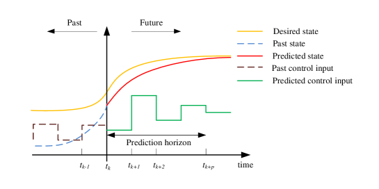
Figure 1: Scheme of receding horizon control.

.

2.3 Mathematical formulation of longitudinal control

2.3.1 State prediction model

The system state x from the perspective of ACC vehicle $n$ is fully described by the gap (net distance headway) $s$, the relative speed $\Delta v$ with respect to its predecessor and its own speed $v$, where $\textbf{x}=(x_{1},x_{2},x_{3})^{T}=(s_{n},\Delta v_{n},v_{n})^{T}$ with $\Delta v_{n}=v_{n-1}-v_{n}$. The system dynamics follow the deterministic kinematic equations:

$${\mathrm{d}\over\mathrm{d}t}\textbf{x}={\mathrm{d}\over\mathrm{d}t}\left(\begin{array}[]{c}s_{n}\\ \Delta v_{n}\\ v_{n}\end{array}\right)=\left(\begin{array}[]{c}\Delta v_{n}\\ u_{n-1}-u_{n}\\ u_{n}\end{array}\right)=\textbf{f}(\textbf{x},\textbf{u})$$ (1)

where $u_{n}$ denotes the acceleration of vehicle $n$, which is the control input in this model. $u_{n-1}$ denotes the acceleration of the predecessor, which equals zero within the prediction horizon based on our assumption. The considered system is a time invariant system, i.e. the system dynamics model f does not depend explicitly on time $t$.

Notice that when applying the controller, other vehicles may not travel at constant speed, which implies a mismatch between the prediction model and the system due to the constant-speed heuristic. The feedback nature of the receding horizon process, which entails reassessing the control input at regular time intervals $\Delta t$ with the newest information of other vehicles, is permanently corrected, and thus robust to the mismatch.

For Cooperative ACC (C-ACC) controllers, the system state for vehicle $n$ is extended to include the situation of its follower $n+1$, $\textbf{x}=(s_{n},\Delta v_{n},v_{n},s_{n+1},\Delta v_{n+1},v_{n+1})^{T}$, where $s_{n+1},\Delta v_{n+1}$ and $v_{n+1}$ denote the gap, relative speed and speed of the follower of the controlled vehicle respectively. The system dynamics now follow:

$${d\over dt}\textbf{x}={d\over dt}\left(\begin{array}[]{c}s\\ \Delta v_{n}\\ v_{n}\\ s_{n+1}\\ \Delta v_{n+1}\\ v_{n+1}\end{array}\right)=\left(\begin{array}[]{c}\Delta v_{n}\\ u_{n-1}-u_{n}\\ u_{n}\\ \Delta v_{n+1}\\ u-u_{v}\\ u_{n+1}\end{array}\right)=\textbf{f}(\textbf{x},\textbf{u})$$ (2)

with $u_{n+1}$ denoting the acceleration of the follower. $u_{n-1}$ and $u_{n+1}$ equal zero within the prediction horizon.

2.3.2 Cost formulation

We formulate the cost of car following, given that the control input $\textbf{u}=\{u_{n}(\tau)|\tau\geq t_{k}\}$ is applied , using the following functional:

$$J(t_{k},\textbf{x}|\textbf{u})=\int_{t_{k}}^{t_{k}+T_{p}}e^{-\eta\tau}{\cal L}(\textbf{x},\textbf{u},\tau)d\tau+e^{-\eta(t_{k}+T_{p})}\phi(\textbf{x}(t_{k}+T_{p}))$$ (3)

with $T_{p}$ denoting the prediction horizon. The cost functional $J(t_{k},\textbf{x}|\textbf{u})$ describes the expected cost (or disutility) given the current state of the system $\textbf{x}(t_{k})$, the control input u and the evolution of the system, starting from the current time $t_{k}$ to terminal time $t_{k}+T_{p}$. In Eq. (3), $\cal{L}$ denotes the so-called running cost, describing the cost incurred during an infinitesimal period $[\tau,\tau+d\tau)$, which are additive over time. $\phi$ denotes the so-called terminal cost, which reflects the cost remaining at the terminal time.

The parameter $\eta\geq 0$ with a unit of $s^{-1}$ denotes the so-called discount factor (Fleming and Soner, 1993), which reflects some trade-off between cost incurred in the near term and future cost. $\eta=0$ implies that the controller weighs the future cost similar to the current cost, which may be the case if the controller can predict the dynamics of the predecessor behaviour fairly well. $\eta>>0$ results in a short-sighted driving behaviour where the controller optimises the immediate situation and does not care too much about the future. Particularly, the cost after a future horizon $[0,\frac{1}{\eta})$ decreases exponentially.

Notice that if $\eta=0$ and $T_{p}<\infty$, the considered problem pertains to a finite horizon optimal control problem with un-discounted cost (e.g., Fleming and Soner, 1993). Solving this type of problem entails choosing a terminal cost $\phi$ to ensure expected controller behaviour and computational feasibility, which is not trivial (Chen and Allgower, 1998). An alternative is to set $\eta>0$ and $T_{p}=\infty$, thus the weight for the terminal cost $e^{-\eta T_{p}}$ equals zero. This removes the parameter $T_{p}$ and relieves us from defining a terminal cost $\phi$. The considered problem becomes an infinite horizon optimal control problem with discounted cost (e.g., Fleming and Soner, 1993).

In the present work, we choose the infinite horizon problem with discounted cost. The optimal control problem is now described by the following mathematical program:

$$\textbf{u}_{[t_{k},\infty)}^{*}=\arg\min J(t_{k},\textbf{x}|\textbf{u})=\arg\min\int_{t_{k}}^{\infty}e^{-\eta\tau}{\cal L}(\textbf{x},\textbf{u})d\tau$$ (4)

subject to:

$${\mathrm{d}\over\mathrm{d}t}\textbf{x}=f(\textbf{x},\textbf{u})$$ (5)

The control input u will be re-assessed at regular time intervals $\Delta t=t_{k+1}-t_{k}$ using the most current observations or estimates of the system state (at time $t_{k+1}$).

Notice that in this contribution we consider multiple criteria for the optimisation, i.e. safety, efficiency, and comfort, but transform the supported driving task into a single-objective mathematical optimisation problem (Eqs (4, 5)) by assuming fixed weights for different criteria.

2.4 Solution approach based on Dynamic Programming

Here we briefly discuss the solution to the considered problem of Eqs. (4, 5), based on the well-known dynamic programming approach.

Let us denote $W(t_{k},\textbf{x})$ as the so-called $valuefunction$, which is the optimal cost function under optimal control $\textbf{u}^{*}$:

$$W(t_{k},\textbf{x})=J(t_{k},\textbf{x}|\textbf{u}^{*})$$ (6)

Applying Bellman’s Principle of Optimality yields the Hamilton-Jacobi-Bellman (HJB) equation with discount factor as (Fleming and Soner, 1993):

$$\eta W(\textbf{x})={\cal H}\left(\textbf{x},\textbf{u}^{*},\frac{\partial W(\textbf{x})}{\partial\textbf{x}}\right)$$ (7)

where $\cal{H}$ is the so-called Hamilton equation (Hamiltonian), which satisfies:

$${\cal H}\left(\textbf{x},\textbf{u}^{*},\frac{\partial W(\textbf{x})}{\partial\textbf{x}}\right)=\underset{\textbf{u}}{\min}\left({\cal L}+\frac{\partial W(\textbf{x})}{\partial\textbf{x}}\cdot\textbf{f}\right)$$ (8)

Let $\boldsymbol{\lambda}=\frac{\partial W(\textbf{x})}{\partial\textbf{x}}$ denote the so-called co-state or marginal cost of the state x, reflecting the relative extra cost of $W$ due to making a small change $\delta\textbf{x}$ on the state x. Taking the partial derivative of Eq. (7) with respect to state x gives:

$$\boldsymbol{\lambda}=\frac{1}{\eta}\frac{\partial\cal H}{\partial\textbf{x}}=\frac{1}{\eta}\frac{\partial\cal{L}}{\partial\textbf{x}}+\frac{1}{\eta}\frac{\partial(\boldsymbol{\lambda}\cdot\textbf{f})}{\partial\textbf{x}}$$ (9)

Using the Hamiltonian of Eq. (8), we can derive the following necessary condition for the optimal control $\textbf{u}^{*}$:

$${\cal H}(\textbf{x},\textbf{u}^{*},\boldsymbol{\lambda})\leq{\cal H}(\textbf{x},\textbf{u},\boldsymbol{\lambda}),\hskip 7.11317pt\forall\textbf{u}$$ (10)

In nearly all cases, this requirement will enable expressing the optimal control $\textbf{u}^{*}$ as a function of the state x and the co-state $\boldsymbol{\lambda}$.

Taking the necessary condition of $\frac{\partial\cal H}{\partial\textbf{u}}=0$ gives the following optimal control law for ACC vehicle $n$:

$$\textbf{u}^{*}=\lambda^{\Delta v_{n}}-\lambda^{v_{n}}$$ (11)

where $\lambda^{\Delta v_{n}}$ and $\lambda^{v_{n}}$ denote the co-state of relative speed and the co-state of speed respectively, and are given by:

$$\lambda^{\Delta v_{n}}=\frac{1}{\eta}\frac{\partial{\cal L}}{\partial\Delta v_{n}}+\frac{1}{\eta^{2}}\frac{\partial{\cal L}}{\partial s_{n}}\mbox{ , }\lambda^{v_{n}}=\frac{1}{\eta}\frac{\partial{\cal L}}{\partial v_{n}}-\frac{1}{\eta^{2}}\frac{\partial{\cal L}}{\partial s_{n}}$$ (12)

The optimal acceleration control law (11) states that the automated vehicle will increase its speed when the marginal cost of relative speed is larger than the marginal cost of speed, and decelerate when vice versa.

For the C-ACC controller, the change in the system state and dynamics results in the following optimal control law when applying the same solution approach:

$$\textbf{u}^{*}=\lambda^{\Delta v_{n}}-\lambda^{v_{n}}-\lambda^{\Delta v_{n+1}}$$ (13)

with $\lambda^{\Delta v_{n}}$ and $\lambda^{v_{n}}$ given in (12) and

$$\lambda^{\Delta v_{n+1}}=\frac{1}{\eta}\frac{\partial{\cal L}}{\partial\Delta v_{n+1}}+\frac{1}{\eta^{2}}\frac{\partial{\cal L}}{\partial s_{n+1}}$$ (14)

Equation (13) shows that the optimal acceleration for a C-ACC vehicle is determined by the marginal costs of its relative speed and speed, as well as the marginal cost of the relative speed of its follower. Clearly, the inclusion of marginal cost of the follower’s speed in the optimal control law captures the cooperative nature of the C-ACC controller.

We emphasise that the control input u is not limited to the control of a single vehicle. The framework allows simultaneous control of multiple vehicles, i.e. two controlled vehicles in a cooperative system.

2.5 Example 1: ACC model

As a first example, we present an ACC model that is collision-free and can generate plausible human driving behaviour using the proposed control framework.

2.5.1 Cost specification and optimal acceleration

We distinguish between cruising (free driving) mode and following mode for the proposed ACC system. In cruising mode, ACC vehicles try to travel at a user defined free speed $v_{0}$. In following mode, ACC vehicles try to maintain a gap-dependent desired speed $v_{d}$ while at the same time avoiding driving too close to the predecessor. For the sake of notation simplicity, we will drop the index $n$ in the ACC controller. Mathematically, the two-regime running cost function can be formulated as:

$${\cal L}=\left\{\begin{array}[]{cl}{\underbrace{c_{1}e^{\frac{s_{0}}{s}}\Delta v^{2}\cdot\Theta(\Delta v)}_{safety}+\underbrace{c_{2}(v_{d}(s)-v)^{2}}_{efficiency}+\underbrace{\frac{1}{2}u^{2}}_{comfort}}&\mbox{ if }s\leq s_{f}=v_{0}\cdot t_{d}+s_{0}\\ {\underbrace{c_{3}(v_{0}-v)^{2}}_{efficiency}+\underbrace{\frac{1}{2}u^{2}}_{comfort}}&\mbox{ if }s>s_{f}=v_{0}\cdot t_{d}+s_{0}\\ \end{array}\right.$$ (15)

where $s_{f}$ is the gap threshold to distinguish cruising mode ($s>s_{f}$) from following mode ($s\leq s_{f}$) and is calculated with $s_{f}=v_{0}\cdot t_{d}+s_{0}$, where $v_{0}$ is the free speed and $s_{0}$ is the distance between two cars at completely congested (standstill) conditions. $t_{d}$ denotes the user-defined desired time gap. $v_{d}(s)$ is the so-called desired speed in following mode and is determined by :

$$v_{d}(s)=\frac{s-s_{0}}{t_{d}}$$ (16)

$\Theta$ is a delta function which follows the form:

$$\Theta(\Delta v)=\left\{\begin{array}[]{cl}{1}&\mbox{ if $\Delta v\leq 0$}\\ {0}&\mbox{ if $\Delta v>0$}\\ \end{array}\right.$$ (17)

Equation (15) implies that the controller makes some trade-off among the safety cost, efficiency cost and comfort cost when following a preceding vehicle:

• The safety cost only incurs when approaching the preceding vehicle, i.e. $\Delta v<0$; $c_{1}>0$ is a constant weight factor. The exponential term $e^{\frac{s_{0}}{s}}$ of the safety cost ensures a large penalty when driving too close to the predecessor, i.e. $s\leq s_{0}$. The safety cost is a monotonic decreasing function of gap $s$, reflecting the fact that the sensitivity to the relative speed tends to decrease with the increase of following distance. There is no safety cost in cruising mode.

• The efficiency cost term in following mode incurs deviating from the desired speed; $c_{2}>0$ is a constant weight factor. The user-set desired time gap $t_{d}$ reflects driver preference and driving style, i.e. a smaller $t_{d}$ tends to an aggressive driving style, while a larger one means more timid driving behaviour. This cost also stems from the interaction with the predecessor, and will not appear in the cruising mode.

• The travel efficiency cost in cruising mode stems from not driving at free speed $v_{0}$, with a constant weight $c_{3}>0$.

• The comfort cost is represented by penalising accelerating or decelerating behaviour.

Employing the solution of Eq. (11) arrives at the following optimal control law:

$$u^{*}=\left\{\begin{array}[]{cl}{\frac{2c_{1}e^{\frac{s_{0}}{s}}}{\eta}\left(\Delta v-\frac{s_{0}\Delta v^{2}}{\eta s^{2}}\right)\cdot\Theta(\Delta v)+\frac{2c_{2}}{\eta}\left(1+\frac{2}{\eta t_{d}}\right)\left(v_{d}(s)-v\right)}&\mbox{ if $s\leq s_{f}$}\\ \frac{2c_{3}}{\eta}{(v_{0}-v)}&\mbox{ if $s>s_{f}$}\\ \end{array}\right.$$ (18)

Equation (18) shows that the optimal acceleration is a function of the state $\textbf{x}=(s,\Delta v,v)^{T}$. The first term in following mode (when $s\leq s_{f}$) describes the tendency to decelerate when approaching the predecessor, while the second term describes the tendency to accelerate when the vehicle speed is lower than the desired speed and the tendency to decelerate when vice versa. In cruising mode ACC vehicles adjust their speed towards the free speed $v_{0}$ to minimise the efficiency cost, with an acceleration proportional to the speed difference with respect to the free speed.

In reality, the accelerations of vehicles are usually limited by the power train, i.e. $u\leq 2m/s^{2}$. For the optimal acceleration function (18), it achieves its maximum $u^{*}_{max,f}$ in following mode when $s=s_{f}$, $v=0km/h$, and $\Delta v\geq 0km/h$ and achieves its maximum $u^{*}_{max,c}$ in cruising mode when $v=0km/h$ for all $s>s_{f}$ and $\Delta v$:

$$u^{*}_{max,f}=u(s_{f},\Delta v,0)=\frac{2c_{2}v_{0}}{\eta}(1+\frac{2}{\eta t_{d}})\mbox{ , for $\Delta v\geq 0$}$$ (19)

and

$$u^{*}_{max,c}=a^{*}(s,\Delta v,0)=\frac{2c_{3}v_{0}}{\eta}\mbox{ , for $s>s_{f}$}$$ (20)

To smooth the transition from following mode to cruising mode, we let $u^{*}_{max,f}=u^{*}_{max,c}$, which leads to the following relationship between the two weights:

$$c_{3}=c_{2}(1+\frac{2}{\eta t_{d}})$$ (21)

In doing so, the total number of parameters in the model has been reduced. The default parameters of the model are shown in Table 1.

2.5.2 Verification of the ACC model

To verify whether the proposed ACC model generates plausible human car-following behaviour, we check the mathematical property of the acceleration function (18) and perform a face validation of the ACC model. Several authors have provided basic requirements for plausible car-following models (Treiber and Kesting, 2011; Wilson and Ward, 2011). Let $u_{mic}(s,\Delta v,v)$ denote a general class of car-following models where the acceleration is a function of gap $s$, relative speed $\Delta v$ and speed $v$. The basic requirements for car-following models can be summarised with:

1. The acceleration is an increasing function of the gap to the predecessor $\frac{\partial u_{mic}(s,\Delta v,v)}{\partial s}\geq 0$ and is not influenced by the gap when the predecessor is far in front: $\lim_{s\to\infty}\frac{\partial u_{mic}(s,\Delta v,v)}{\partial s}=0$.

2. The acceleration is an increasing function of relative speed with respect to the preceding vehicle $\frac{\partial u_{mic}(s,\Delta v,v)}{\partial\Delta v}\geq 0$, and is not influenced by the relative speed at very large gaps $\lim_{s\to\infty}\frac{\partial u_{mic}(s,\Delta v,v)}{\partial\Delta v}=0$.

3. The acceleration is a strictly decreasing function of speed $\frac{\partial u_{mic}(s,\Delta v,v)}{\partial v}<0$, and equals zero when vehicles travel with free speed at very large gaps $\lim_{s\to\infty}u_{mic}(s,\Delta v,v_{0})=0$.

It can be shown that the proposed optimal ACC control law of Eq. (18) satisfies the three basic requirements.

Fig. 2 shows the contour plot of the optimal acceleration for different gaps and relative speeds when following a predecessor driving constantly with a speed of $54km/h$ using default parameters. Clearly we can see the two regimes of following mode and cruising mode distinguished at the gap of around $35m$. At cruising mode, the acceleration is above zero, because all the possible speeds (between $36km/h$ and $72km/h$) in the contour plot are below the free speed of $120km/h$. In following mode, the acceleration increases with the increase of headway and relative speed, and consequently decreases with the increase of vehicle speed. The thick line between the green and yellow area shows the neutral line where the accelerations equal zero. Most of the left plane in following mode show a negative acceleration, as a result of the safety cost. This asymmetric property of the optimal acceleration prevents vehicles from driving too close to the leader.

Fig. 2 shows how the system evolves from a high cost area to a low cost area of an ACC vehicle following a predecessor driving constantly with a speed of $54km/h$. The initial state is $s=15m$ and $\Delta v=-14km/h$ ($v=68km/h$), denoted with ’O’ in the figure, using the default parameters. The contour lines show the cost, while the dark star line shows the trajectory of the vehicle, with the optimal acceleration evaluated every $0.25s$. At the start, the ACC controller incurred safety cost due to approaching the leader and travel efficiency cost due to driving higher than the desired speed of around $47km/h$. The vehicle starts to decelerate until the relative speed is $0km/h$. Then it continues to decelerate because driving at $54km/h$ is still higher than the desired speed, which has changed to around $36km/h$ (at the gap of $12m$). As a result, the vehicle will travel with a lower speed and the gap to the predecessor will increase, leading to an increase of the desired speed. The vehicle starts to accelerate when the desired speed is higher than the vehicle speed. The trade-off between the travel efficiency and safety cost will finally lead to the behaviour as shown in the figure, ending with ’D’ in the figure after a simulation period of $50s$.

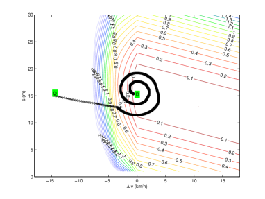
Figure 2: (a) Contour plot of optimal acceleration when following a vehicle driving at $54km/h$; (b) Contour plot of optimal cost with a vehicle trajectory.

.

Table 1: Model parameters

Parameter	Physical meaning	Default value	Unit
$v_{0}$	free speed	120	$km/h$
$c_{1}$	weight on safety cost	0.1	$s^{-2}$
$c_{2}$	weight on efficiency cost	0.001	$s^{-2}$
$\eta$	discount factor	0.25	$s^{-1}$
$t_{d}$	desired time gap	1.0	$s$
$s_{0}$	desired gap at standstill	1	$m$
$l$	vehicle length	5	$m$

2.6 Example 2: Cooperative-ACC model

As a second example, we apply the control framework to design Cooperative-ACC (C-ACC) systems where the controlled vehicle does not only consider its own situation but also the situation of its follower when making control decisions. The cooperation mechanism is applied when one C-ACC vehicle is followed by another C-ACC vehicle. In that situation, the two C-ACC vehicles exchange their gaps and relative speeds with each other through V2V communications and they collaborate to minimise a joint cost function, reflecting the situation of both C-ACC vehicles.

2.6.1 Joint running cost function for C-ACC

The cooperative behaviour entails minimising a joint cost. Since there is no interaction in cruising mode, we assume that the cooperative behaviour only occurs when both the controlled vehicle and its follower are operating in following mode. Thus we only change the running cost at following mode, which becomes:

$${\cal L}=c_{1}\sum\limits_{j=n}^{n+1}e^{\frac{s_{0}}{s_{j}}}\Delta v_{j}^{2}\cdot\Theta(\Delta v_{j})+c_{2}\sum\limits_{j=n}^{n+1}(v_{j}-v_{d}(s_{j}))^{2}+\frac{1}{2}\sum\limits_{j=n}^{n+1}u_{j}^{2}$$ (22)

The running cost function (22) shows that in following mode, the cooperative controller aims to minimising the acceleration, safety cost due to approaching the preceding vehicle and efficiency cost due to not driving at desired speed of the C-ACC vehicle and its follower.

2.6.2 Optimal control of C-ACC vehicles

Following solution (13), we arrive at:

$$u^{*} = \frac{2c_{1}e^{\frac{s_{0}}{s_{n}}}}{\eta}\left(\Delta v_{n}-\frac{s_{0}\Delta v_{n}^{2}}{\eta s_{n}^{2}}\right)\cdot\Theta(\Delta v_{n})+\frac{2c_{2}}{\eta}(1+\frac{2}{\eta t_{d}})\left(v_{d}(s_{n})-v_{n}\right)$$ (23)

$${}-\frac{2c_{1}e^{\frac{s_{0}}{s_{n+1}}}}{\eta}\left(\Delta v_{n+1}-\frac{s_{0}\Delta v_{n+1}^{2}}{2\eta s_{n+1}^{2}}\right)\cdot\Theta(\Delta v_{n+1})-\frac{2c_{2}}{\eta^{2}t_{d}}(v_{d}(s_{n+1})-v_{n+1})$$

In Eq. (23), the optimal acceleration of a C-ACC vehicle $n$ is a function of gap, relative speed and speed of both itself and its follower (vehicle $n+1$). The first two terms in Eq. (23) correspond to the non-cooperative ACC model in Eq. (18). The third term shows that the C-ACC vehicle will accelerate when its follower is approaching. The fourth term implies that the C-ACC vehicle tends to decelerate when the follower is travelling below the desired speed and tends to accelerate when vice versa. In doing so, the joint cost function (22) is optimised. The backward-looking behaviour in the third and fourth term shows how the follower’s situation affects the optimal control.

3 Equilibrium solutions and stability analysis

In this section, we present the method for analysing ADAS model characteristics, with a focus on equilibrium solution and linear stability analysis. Particularly, we consider a more generalised expression of the optimal controller with cooperative behaviour. The acceleration is expressed as a function of gap, relative speed, and speed of the controlled vehicle $n$ and its follower vehicle $n+1$:

$$u_{n}(s_{n},\Delta v_{n},v_{n},s_{n+1},\Delta v_{n+1},v_{n+1}).$$

3.1 Equilibrium solutions

At equilibria in homogeneous traffic, all vehicles travel at the same speed with the same gap and zero acceleration. The equilibrium solutions are derived by the following equation:

$$u_{n}(s_{e},0,v_{e},s_{e},0,v_{e})=0$$ (24)

which gives a unique equilibrium speed as a function of gap $v_{e}(s_{e})$, or an equilibrium gap as a function of speed $s_{e}(v_{e})$.

3.2 Linear stability analysis

The stability analysis framework generalises the classic linear stability analyses approach (Holland, 1998; Treiber and Kesting, 2011; Wilson and Ward, 2011) to cooperative systems. Effects on string stability of the cooperative behaviour can be analytically derived. Types of convective instability are classified using signs of signal velocity with a simpler calculation procedure compared to the method of Ward and Wilson (2011).

Let us assume a small deviation $h_{n}$ and $g_{n}$ of the $n$th vehicle in the homogeneous platoon from the steady-state gap $s_{e}$ and speed $v_{e}$ respectively, then the gap and speed of vehicle $n$ can be written as:

$$s_{n}=s_{e}+h_{n}\mbox{ , }v_{n}=v_{e}+g_{n}$$ (25)

The first and second order derivatives of $h_{n}$ give:

$$\dot{h}_{n}=\Delta v_{n}=g_{n-1}-g_{n}\mbox{ , }\ddot{h}_{n}=u_{n-1}-u_{n}$$ (26)

Approximating $u_{n-1}$ and $u_{n}$ in Eq. (26) around equilibria using Taylor series to the first order arrives at:

$$\ddot{h}_{n} = u_{s}(h_{n-1}-h_{n})+u_{\Delta v}(\dot{h}_{n-1}-\dot{h}_{n})+u_{v}\dot{h}_{n}$$ (27)

$${}+u_{s_{b}}(h_{n}-h_{n+1})+u_{\Delta v_{b}}(\dot{h}_{n}-\dot{h}_{n+1})+u_{v_{b}}\dot{h}_{n+1}$$

with the coefficients (gradients of acceleration) evaluated at equilibria:

$$u_{s}=\frac{\partial u_{n}}{\partial s_{n}}|_{e}\mbox{ , }u_{\Delta v}=\frac{\partial u_{n}}{\partial\Delta v_{n}}|_{e}\mbox{ , }u_{v}=\frac{\partial u_{n}}{\partial v_{n}}|_{e}\mbox{ , }u_{s_{b}}=\frac{\partial u_{n}}{\partial s_{n+1}}|_{e}\mbox{ , }u_{\Delta v_{b}}=\frac{\partial u_{n}}{\partial\Delta v_{n+1}}|_{e}\mbox{ , }u_{v_{b}}=\frac{\partial u_{n}}{\partial v_{n+1}}|_{e}$$

The equilibrium solutions $v_{e}(s_{e})$ restrict the coefficients from being independent from each other. The acceleration and relative speed along the equilibrium solutions should always be zero. This property leads to the following relationship by approximating acceleration around equilibria with Taylor expansion to the first order:

$$(u_{s}+u_{s_{b}})=-v_{e}^{\prime}(s_{e})\cdot(u_{v}+u_{v_{b}})$$ (28)

3.2.1 Local stability criteria

For local stability, we are primarily interested in a pair of vehicles, where the leader is driving constantly. In this case, Eq. (27) will relax to:

$$\ddot{h}_{n}+(u_{\Delta v}-u_{v})\dot{h}_{n}+u_{s}h_{n}=0$$ (29)

Equation (29) is a harmonic damped oscillator which can be solved using the following ansatz:

$$h=h_{0}e^{\gamma t}$$ (30)

where $\gamma=\sigma+i\omega$ ($i=\sqrt{-1}$) is the complex growth rate and $h_{0}$ reflects the amplitude of the initial disturbance. We can reformulate the damped oscillator as:

$$\gamma^{2}+\left(u_{\Delta v}-u_{v}\right)\gamma+u_{s}=0$$ (31)

with solutions

$$\gamma_{1,2}=\frac{-(u_{\Delta v}-u_{v})\pm\sqrt{(u_{\Delta v}-u_{v})^{2}-4u_{s}}}{2}$$ (32)

Local stability requires both solutions of Eq. (31), $\gamma_{1}$ and $\gamma_{2}$, to have negative real parts, which is satisfied by the following condition:

$$u_{\Delta v}-u_{v}>0$$ (33)

3.2.2 String stability criteria

For string stability, we are interested in how a small disturbance propagates through the increasing index of vehicles. We state the following theorem for string stability of generalised driver assistance system controllers in the form of (3).

Theorem 1 If $u_{v}+u_{v_{b}}<0$, string stability is guaranteed by the inequality:

$$v_{e}^{\prime}(s_{e})^{2}\leq v_{e}^{\prime}(s_{e})(u_{\Delta v}+u_{\Delta v_{b}}-u_{v_{b}})+\frac{u_{s}-u_{s_{b}}}{2}$$ (34)

Proof The generalised disturbance dynamic equation of (27) can be solved using Fourier analysis with the following ansatz:

$$h_{n}=h_{0}e^{\gamma t+ink}\mbox{ , }g_{n}=g_{0}e^{\gamma t+ink}$$ (35)

where $\gamma=\sigma+i\omega$ ( $i=\sqrt{-1}$) is the complex growth rate. The real part $\sigma$ denotes the growth rate of the oscillation amplitude while the imaginary part $\omega$ is the angular frequency from the perspective of the vehicle. The dimensionless wave number $k\in(-\pi,\pi)$ indicates the phase shift of the traffic waves from one vehicle to the next at a given time instant, and the corresponding physical wavelength is $2\pi(s_{e}+l)/k$ (Treiber and Kesting, 2010).

To find the limit for string instability, we insert Eq. (35) into Eq. (27), which yields the following quadratic equation of the eigenvalue $\gamma$:

$$\gamma^{2}+p(k)\gamma+q(k)=0$$ (36)

for the complex growth rate $\gamma$ given by

$$\gamma_{\pm}(k)=-\frac{p(k)}{2}\pm\frac{\sqrt{p^{2}(k)-4q(k)}}{2}$$ (37)

with coefficients:

$$p(k)=u_{\Delta v}(1-e^{-ik})-u_{v}+u_{\Delta v_{b}}(e^{ik}-1)-u_{v_{b}}e^{ik}\mbox{ , }q(k)=u_{s}(1-e^{-ik})+u_{s_{b}}(e^{ik}-1)$$ (38)

For a given wave number $k$, only two complex growth rates $\gamma_{+}$ and $\gamma_{-}$ are possible and $\mathrm{Re}(\gamma_{+})\geq\mathrm{Re}(\gamma_{-})$. The model is string stable if $\mathrm{Re}(\gamma)<0$ for both solutions and for all wave numbers (relative phase shifts) in the range $k\in[-\pi,\pi]$.

It can be proven that the first instability of time-continuous car-following models without explicit delay always occurs for wave number $k\to 0$ (Wilson, 2008). Thus we can expand coefficients of the $p(k)$ and $q(k)$ with Taylor series around $k=0$:

$$p(k)=p_{0}+p_{1}k+\mathcal{O}(k^{2})\mbox{ , }q(k)=q_{1}k+q_{2}k^{2}+\mathcal{O}(k^{3})$$ (39)

with

$$p_{0}=p(0)=-u_{v}-u_{v_{b}}\mbox{ , }p_{1}=p^{\prime}(0)=i(u_{\Delta v}+u_{\Delta v_{b}}-u_{v_{b}})$$

$$q_{1}=q^{\prime}(0)=i(u_{s}+u_{s_{b}})=iv^{\prime}_{e}(s_{e})p_{0}\mbox{ , }q_{2}=\frac{q^{\prime\prime}(0)}{2}=\frac{u_{s}-u_{s_{b}}}{2}$$ (40)

Expanding root $\gamma_{+}$ around $k=0$ to second order of $k$ and using the Taylor series of square root of $\sqrt{1-\epsilon}=1-\epsilon/2-\epsilon^{2}/8+\mathcal{O}(\epsilon^{3})$ gives:

$$\gamma_{+}=-\frac{q_{1}}{p_{0}}k+\left(\frac{q_{1}p_{1}}{p_{0}^{2}}-\frac{q_{2}}{p_{0}}-\frac{q_{1}^{2}}{p_{0}^{3}}\right)k^{2}+\mathcal{O}(k^{3})$$ (41)

Notice that the first term in Eq. (41) is purely imaginary and the second term is a real number. String stability is governed by the sign of the second term. For string stability, it is required that:

$$\frac{q_{1}p_{1}}{p_{0}^{2}}-\frac{q_{2}}{p_{0}}-\frac{q_{1}^{2}}{p_{0}^{3}}\geq 0$$ (42)

If $u_{v}+u_{v_{b}}<0$, which implies $p_{0}>0$, moving the last term in the inequality to the right side and multiply $p_{0}$ will give:

$$\frac{q_{1}^{2}}{p_{0}^{2}}\leq\frac{q_{1}p_{1}}{p_{0}}-q_{2}$$ (43)

Replacing the coefficients with Eqs. (40) in the inequality (42) and divide by $p_{0}^{2}$ will give:

$$v_{e}^{\prime}(s_{e})^{2}\leq v_{e}^{\prime}(s_{e})(u_{\Delta v}+u_{\Delta v_{b}}-u_{v_{b}})+\frac{u_{s}-u_{s_{b}}}{2}$$ (44)

Q.E.D.

For ACC systems that only reacts to the direct predecessor, the string stability criteria relax to:

$$v_{e}^{\prime}(s_{e})^{2}\leq v_{e}^{\prime}(s_{e})u_{\Delta v}+\frac{u_{s}}{2}$$ (45)

When comparing Eq. (34) with Eq. (45), we can draw the following analytical criteria for stabilisation effects of cooperative systems. If a cooperative system keeps the equilibrium speed-gap relationship and the gradients of acceleration $u_{s}$, $u_{\Delta v}$ and $u_{v}$ the same as a non-cooperative system, the stabilisation effect of the cooperative behaviour compared to the non-cooperative model, is determined with:

$$v_{e}^{\prime}(s_{e})(u_{\Delta v_{b}}-u_{v_{b}})-\frac{u_{s_{b}}}{2}>0\mbox{, cooperative system is more stable;}$$

$$v_{e}^{\prime}(s_{e})(u_{\Delta v_{b}}-u_{v_{b}})-\frac{u_{s_{b}}}{2}=0\mbox{, model stability criteria remains unchanged;}$$

$$v_{e}^{\prime}(s_{e})(u_{\Delta v_{b}}-u_{v_{b}})-\frac{u_{s_{b}}}{2}<0\mbox{, cooperative system is more unstable.}$$ (46)

3.2.3 Convective instability

Several authors discovered that the flow instability in traffic flow are of a convective type (Wilson and Ward, 2011; Treiber and Kesting, 2011). Let $Z(x,t)$ denote the spatio-temporal evolution of an initial perturbation $Z(x,0)$. Traffic flow is convectively unstable if it is linearly unstable and if

$$\lim\limits_{t\to\infty}Z(0,t)=0$$ (47)

Intuitively, Eq. (47) means that the perturbation will eventually convect out of the system after a sufficient time (Wilson and Ward, 2011; Treiber and Kesting, 2011). Otherwise, if traffic flow is linearly unstable but does not satisfy Eq. (47), then it is absolutely unstable.

To investigate the limits of convective instability, Treiber and Kesting (2010) proposed Fourier transform of a linear response function, which enables one to determine the spatio-temporal evolution of the perturbation $Z(x,t)$. The approach involves finding the wave number corresponding to the maximum growth rate and expanding the complex growth rate around the wave number. After solving a well-defined Gaussian integral, one can obtain the spatio-temporal evolution of the perturbation as:

$$Z(x,t)=\mathrm{Re}\frac{Z_{0}}{\sqrt{-2\pi\gamma^{\prime\prime}(k^{p}_{0})t}}\exp\left[i(k^{p}_{0}x-\omega^{p}_{0}t)\right]\exp\left[\left(\sigma_{0}+\frac{(c_{g}-\frac{x}{t})^{2}}{2(i\omega^{p}_{kk}-\sigma^{p}_{kk})}\right)t\right]$$ (48)

where $k_{0}^{p}$ denotes the physical wave number with the maximum growth rate, and is determined by the dimensionless wave number $k_{0}$:

$$k^{p}_{0}=\frac{k_{0}}{s_{e}+l}\mbox{ , }k_{0}=\arg\max_{k}(\mathrm{Re}\mbox{ }\gamma(k))$$ (49)

and

$$\sigma_{0}=\mathrm{Re}\gamma(k_{0})\mbox{ , }\omega^{p}_{0}=\frac{v_{e}k_{0}}{s_{e}+l}+\mathrm{Im}\gamma(k^{p}_{0})\mbox{ , }\sigma^{p}_{kk}=(s_{e}+l)^{2}\mathrm{Re}\gamma^{\prime\prime}(k_{0})\mbox{ , }\omega^{p}_{kk}=(s_{e}+l)^{2}\mathrm{Im}\gamma^{\prime\prime}(k_{0})$$

$$c_{g}=v_{e}+(s_{e}+l)\mathrm{Im}\gamma^{\prime}(k_{0})\mbox{ , }c_{p}=\frac{\omega_{0}}{k_{0}^{p}}=v_{e}+(s_{e}+l)\frac{\mathrm{Im}\gamma(k_{0})}{k_{0}}$$ (50)

For details, we refer to Treiber and Kesting (2010, 2011).

In Eq. (50), $c_{p}$ denotes the phase velocity, which is defined by the movement of points of constant phase. It represents the propagation velocity of a single wave. For human-driven vehicular traffic, the phase velocity $c_{p}$ is of the order of $-15km/h$ in congested traffic (Treiber and Kesting, 2011). $c_{g}$ is the group velocity, with which the overall shape of the wave amplitudes propagates through space (Lighthill, 1965). More intuitively, the middle of a wave group (or perturbation) propagates with group velocity (Treiber and Kesting, 2010). The group velocity can be influenced by several waves.

While group velocity represents the propagation of the centre of a wave group, signal velocity $c_{s}$ is more representative in describing the spatio-temporal dynamics of disturbance in dissipative media like vehicular traffic flow. The signal velocity represents the propagation of waves that neither grow nor decay. It can be calculated using Eq. (48), by considering the growth rate of $Z(x,t)$ along the trajectory of $x=c_{s}t$ and setting it to be zero, which gives:

$$\sigma_{0}-\mathrm{Re}\left(\frac{(c_{g}-c_{s})^{2}}{2\gamma^{\prime\prime}}\right):=\sigma_{0}-\frac{(c_{g}-c_{s})^{2}}{2D_{2}}$$ (51)

where $D_{2}=-\sigma^{p}_{kk}\left(1+\frac{(\omega_{kk}^{p})^{2}}{(\sigma_{kk}^{p})^{2}}\right)$. If there is any string instability, we have two signal velocities:

$$c_{s}^{\pm}=v_{g}\pm\sqrt{2D_{2}\sigma_{0}}$$ (52)

Equation (52) shows that the perturbed region grows spatially at the constant rate of $2\sqrt{2D_{2}\sigma_{0}}$. Convective instability types can be classified as:

• if $c_{s}^{-}<0<c_{s}^{+}$, traffic flow is absolutely string unstable.

• if $c_{s}^{+}<0$, traffic flow is upstream convectively unstable.

• if $c_{s}^{-}>0$, traffic flow is downstream convectively unstable.

Different from the classification method of using group velocity in Treiber and Kesting (2010), convective instabilities are determined by the signs of signal velocities of disturbance, and the calculation procedure of signal velocity is more approachable to traffic community than that in Ward and Wilson (2011).

4 ACC and C-ACC model characteristics

In this section, we use the model analysis framework described in the previous section to examine the characteristics of ACC and C-ACC models. Since there is no interaction with other vehicles in the optimal control input at cruising mode, we emphasize that both local stability and string stability are guaranteed in cruising mode for both the ACC model and the C-ACC model. The stability analyses in the ensuing focus on following mode.

4.1 Fundamental Diagram

For the ACC model (18), following the equilibrium solutions in the previous section (when $\Delta v=0$ and $a^{*}=0$) gives a unique relationship of equilibrium speed and gap:

$$v_{e}=\left\{\begin{array}[]{cl}\frac{s_{e}-s_{0}}{t_{d}}&\mbox{if $s_{e}\leq s_{f}$}\\ v_{0}&\mbox{ if $s_{e}>s_{f}$}\\ \end{array}\right.$$ (53)

Assuming constant vehicle length $l$ and using the relationship between gap and local density $\rho$: $\frac{1000}{\rho}=s+l$, we will get the classic triangular fundamental diagram of the steady-state flow-density relationship as:

$$q=\left\{\begin{array}[]{cl}3.6v_{0}\rho&\mbox{ if $\rho\leq\frac{1000}{v_{0}t_{d}+s_{0}+l}$}\\ \frac{1000-(s_{0}+l)\rho}{t_{d}}&\mbox{ if $\rho>\frac{1000}{v_{0}t_{d}+s_{0}+l}$}\\ \end{array}\right.$$ (54)

with $q$ denoting traffic flow in the unit of $veh/h$ and $\rho$ in the unit of $veh/km$.

Fig. 3 shows the steady-state speed-gap relationship and Fig. 3 depicts the equilibrium flow-density relation for two different desired time gaps. The two branches in each of the fundamental diagrams are distinguished by the operating mode of the ACC controller. On the left branch ACC vehicles operate in cruising mode, while at the right branch ACC vehicles operate in following mode. With the default parameter $t_{d}=1.0s$, the resulting flow reaches the capacity of $3050veh/h$ at a critical density of around $25veh/km$, while a desired time gap of $1.5s$ leads to a capacity of $2142veh/h$ at a critical density of around $18veh/km$. The critical density is determined by the gap threshold $s_{f}$. The figures shows that the desired time gap has a strong influence on the capacity.

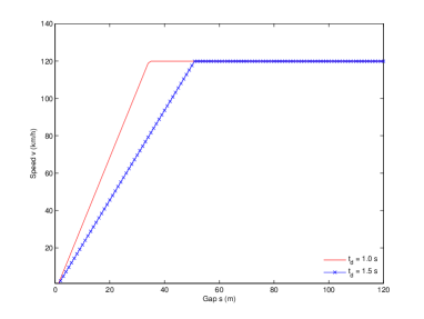
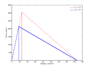
Figure 3: Equilibrium (a) speed-gap relationship and (b) flow-density relationship with $t_{d}=1.0s$ and $t_{d}=1.5s$ and other default parameters in Table 1.

The equilibrium solutions of the C-ACC model are the same as of the new ACC model, and both of them display the fundamental diagram as Eq. (54) and Fig. 3.

4.2 Local stability of the ACC model

Local stability is only interesting for the ACC model. It can be shown with Eq. (18) that in following mode $u^{*}_{\Delta v}>0$ and $u^{*}_{v}<0$, thus the local stability condition (33) is always satisfied. This signifies that the optimal acceleration model of (18) is unconditionally local-stable.

Fig. 4 shows the two roots of linear growth rate $\gamma_{1}$ and $\gamma_{2}$ calculated with solution (32). We can clearly see from the figure that the real parts of the two roots are below zero.

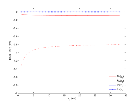
Figure 4: Real and imaginary parts of two roots for local stability of the ACC model with default parameters.

4.3 String stability of the ACC model

String stability of the proposed ACC model is examined with the linear stability approach.

4.3.1 String stability threshold

To find the string stability threshold, we evaluate the gradients of $u^{*}$ (18) at equilibria and the derivative of equilibrium speed in (53) as:

$$u^{*}_{s}=\frac{2c_{2}(2+\eta t_{d})}{\eta^{2}t_{d}^{2}}\mbox{ , }u^{*}_{\Delta v}=\frac{2c_{1}}{\eta}e^{\frac{s_{0}}{s_{e}}}\mbox{ , }u^{*}_{v}=-\frac{2c_{2}\left(2+\eta t_{d}\right)}{\eta^{2}t_{d}}\mbox{ , }v_{e}^{\prime}(s_{e})=\frac{1}{t_{d}}$$ (55)

The stability condition (45) gives the following criteria to guarantee string stability:

$$\frac{2c_{1}t_{d}}{\eta}e^{\frac{s_{0}}{s_{e}}}+c_{2}(\frac{2}{\eta^{2}}+\frac{t_{d}}{\eta})\geq 1$$ (56)

Equation (56) gives the following properties of model parameters on the string stability:

• Increasing safety cost weight $c_{1}$ will stabilise homogeneous flows. Microscopically, a larger $c_{1}$ leads to a higher sensitivity to the relative speed and thus a more anticipative driving style, since relative speed reflects future gaps, which is a simple form of anticipation (Treiber and Kesting, 2010). This explains the stabilisation effects of increasing $c_{1}$.

• Increasing efficiency cost weight $c_{2}$ will stabilise homogeneous flows. A larger $c_{2}$ means that the controller has a higher sensitivity to the deviation from the desired speed. Notice that the maximum acceleration is proportional to $c_{2}$ in Eq. (19), a larger $c_{2}$ means a more responsive agile driving style, which tends to suppress string instabilities (Treiber and Kesting, 2010). However, physical constraints of vehicles limit the choice of too large $c_{2}$, i.e. increasing $c_{1}$ from default value from $0.001s^{-2}$ to $0.002s^{-2}$ with other default parameters already changes the maximum acceleration from $2.5m/s^{2}$ to $5m/s^{2}$.

• Increasing the discount factor $\eta$ will destabilise traffic. Notice that a larger $\eta$ implies a shorter anticipation horizon $\frac{1}{\eta}$, or in other words a more short-sighted driving style. A controller only optimising its immediate situation favours string instability.

• Increasing the desired time gap $t_{d}$ will increase the left hand side of the inequality (56), which implies more stable flow. A larger $t_{d}$ tends to suppress string instability by following with a larger distance at equilibria.

Fig. 5 shows thresholds of stability and instability with different parameters in a two-dimensional parameter plane. The area above the line is string-stable under those parameter settings, while the area below the lines is string-unstable. The stabilisation effects of the parameters are clearly seen.

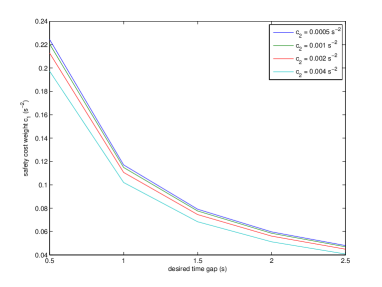
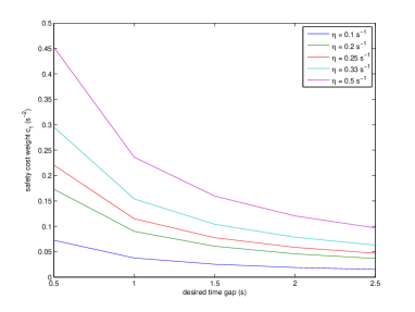
Figure 5: Stability region in a two-dimensional parameter plane of $c_{1}$ and $t_{d}$ with (a) different $c_{2}$ and (b) different $\eta$, under equilibrium speed of 72 $km/h$. Other parameters are default values.

4.3.2 Convective instability

With Eq. (38), the coefficients of the quadratic equation for the complex growth rate $\gamma$ of the ACC model are specified:

$$p(k)=\frac{2c_{1}}{\eta}e^{\frac{s_{0}}{s_{e}}}(1-e^{-ik})+\frac{2c_{2}\left(2+\eta t_{d}\right)}{\eta^{2}t_{d}}\mbox{ , }q(k)=\frac{2c_{2}(2+\eta t_{d})}{\eta^{2}t_{d}^{2}}e^{-ik}$$ (57)

The first and second order derivatives of $p(k)$ and $q(k)$ can be obtained straightforwardly.

The linear stability analysis framework enables one to draw the linear growth rate and the propagation velocities of disturbance for the ACC model as a function of wave number under equilibrium speed of 54 $km/h$, as depicted in Fig. 6. Numerically, we can find the dimensionless wave number $k_{0}$ corresponding to the maximum growth rate with the argument (49), which is 0.082 in this case. The physical wavelength is $(s_{e}+l)2\pi/k_{0}\approx 1.5km$ and the number of vehicles per wave is around $2\pi/k\approx 77$ vehicles. The maximum growth rate is $0.0028s^{-1}$ (the red point in the Fig. 6), which is a slow growth implying that it may take some time for an small disturbance grows to traffic breakdown (Treiber and Kesting, 2010). The phase and group velocity corresponding to this maximum growth rate are $-16km/h$ and $-11km/h$ respectively, with negative sign indicating the propagation direction is against vehicle travelling direction, as depicted in Fig. 6.

Fig. 7 and 7 show the phase, group and signal velocities as a function of equilibrium speed and density respectively. Since traffic is always string stable in cruising mode, traffic flow is always stable below the critical density of $\rho_{c1}=1000/(s_{f}+l)\approx 25veh/km$. As long as the density is higher than the critical density $\rho_{c1}$, traffic becomes absolutely unstable $c_{s+}>0$ and $c_{s-}<0$, with disturbances travelling both upstream and downstream. When the density increases to another critical density $\rho_{c2}\approx 42veh/km$, the traffic becomes convectively upstream unstable, with disturbances travelling upstream only. When the density increases further to above another critical density $\rho_{c3}\approx 96veh/km$, the traffic becomes stable again, which is the so-called restabilisation effect (Treiber and Kesting, 2010). With the default parameters, the ACC model displays absolute and convective upstream instability, which is different from human drivers (Treiber and Kesting, 2010; Wilson and Ward, 2011).

Fig. 7 and 7 show the spatio-temporal evolution of the system using the analytical disturbance function of 48 with different equilibrium speeds of $48km/h$ (density of $52veh/km$) and $72km/h$ (density of $38veh/km$). We can clearly see from the figure that:

• at equilibrium speed of $48km/h$, the initial disturbance travels upstream, while at equilibrium speed of $72km/h$, disturbance travels both upstream and downstream.

• absolute instability grows faster in amplitude, which can be see from the ranges of the speeds contour plots.

• the centre of the disturbance travels with group velocity and each signal wave travels with phase velocity.

• two signal velocities limit the region of disturbance in the spatio-temporal plane.

When choosing different parameters, one can get different stability characteristics of the model. Fig. 8 shows the one dimensional parameter safety cost weight $c_{1}$ and the resulting stability at different equilibrium speeds at following mode with other default parameters. If we increase $c_{1}$ to a slightly higher value than the default one, traffic will become convectively upstream stable and stable in following mode, which is similar to human-driven vehicular traffic. When choosing $c_{1}$ higher than $0.12s^{-2}$, the traffic is always stable, while $c_{1}$ lower than $0.06s^{-2}$ leads to co-existence of convective downstream, absolute and convective upstream instability in the congested branch of the fundamental diagram.

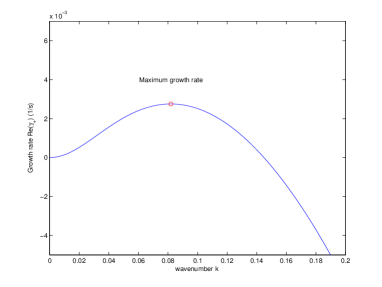
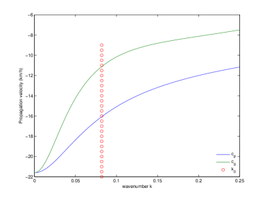
Figure 6: (a) Growth rate of the more unstable branch $\gamma_{+}$ as a function of wave number under $v_{e}=54km/h$ ; (b) phase and group velocity as a function of wave number under $v_{e}=54km/h$ of ACC model with default parameters.

.

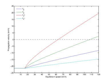
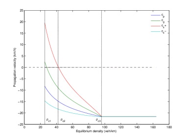
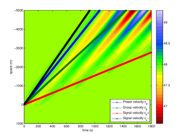
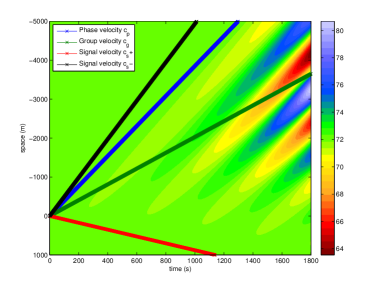
Figure 7: (a) Phase, group, signal velocities as a function of equilibrium speed and (b) phase, group, signal velocities as a function of equilibrium density and spatio-temporal evolution of initial disturbance at equilibrium speed of (c) 48 $km/h$ and (d) 72 $km/h$ of ACC model with default parameters. Driving direction in (c) and (d) is from top to down.

.

4.4 Destabilisation effect of the C-ACC model

The local stability is no longer of interest for the C-ACC controller, since we will consider at least three vehicles in the analysis. For the optimal control of C-ACC controller (23), the gradients are given:

$$u^{*}_{s_{b}}=-\frac{2c_{2}(1+\eta t_{d})}{\eta^{2}t_{d}^{2}}\mbox{ , }u^{*}_{\Delta v_{b}}=-\frac{2c_{1}e^{\frac{s_{0}}{s_{e}}}}{\eta}\mbox{ , }u^{*}_{v_{b}}=\frac{2c_{2}}{\eta^{2}t_{d}}$$ (58)

while $u^{*}_{s}$, $u^{*}_{\Delta v}$, $u^{*}_{v}$ and $v_{e}^{\prime}(s_{e})$ remain the same as in Eq. (55).

Since $u^{*}_{v}+u^{*}_{v_{b}}=<0$, condition (34) gives the following criteria for string stability of C-ACC controller:

$$\frac{c_{2}}{\eta^{2}}(1+\eta t_{d})\geq 1$$ (59)

The stabilisation effect of the C-ACC controller with reference to the ACC controller is governed by (3.2.2). With the virtue of the gradients in Eq. (58) and the analytical criteria for the stabilisation effect of cooperative systems (3.2.2), we found that:

• $u^{*}_{s_{b}}<0$, which stabilises traffic.

• $u^{*}_{\Delta v_{b}}<0$, which destabilises traffic.

• $u^{*}_{v_{b}}>0$, which destabilises traffic.

The total stabilisation effect $v_{e}^{\prime}(s_{e})\left(u^{*}_{\Delta v_{b}}-u^{*}_{v_{b}}\right)-\frac{u^{*}_{s}}{2}=-\frac{2c_{1}}{\eta t_{d}}e^{\frac{s_{0}}{s_{e}}}-\frac{c_{2}}{\eta^{2}t_{d}^{2}}<0$, which implies that the C-ACC controller destabilises homogeneous traffic flow compared to the ACC controller. With default parameters, $|u^{*}_{\Delta v_{b}}|$ is much larger $|u^{*}_{s_{b}}|$ and $|u^{*}_{v_{b}}|$, thus this term deteriorates string stability most.

To classify the convective instability, we need to specify the coefficients of the quadratic equation (36) as:

$$p(k)=u^{*}_{\Delta v}(1-e^{-ik})+u^{*}_{\Delta v_{b}}(e^{ik}-1)-u^{*}_{v}-u^{*}_{v_{b}}e^{ik}\mbox{ , }q(k)=u^{*}_{s}(1-e^{-ik})+u^{*}_{s_{b}}(e^{ik}-1)$$ (60)

The first and second order derivatives of $p(k)$ and $q(k)$ can be obtained straightforwardly.

The linear stability analysis framework enables us to calculate signal velocity at different equilibrium speeds and different parameter settings. Fig. 8 shows the resulting stability/instability types of one dimensional parameters. It is quite clear that the C-ACC controller (23) is much more unstable compared to the ACC controller in Fig. 8. Homogeneous traffic flow is always unstable in following mode, and the instability is of absolute and convective downstream type.

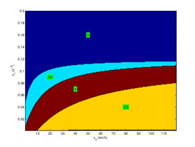
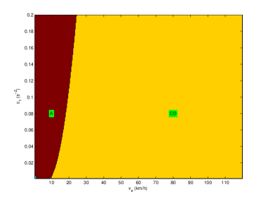
Figure 8: Stability plot with safety cost weight $c_{1}$ and equilibrium speed of (a) ACC model; (b) C-ACC model. S: Stable region; U: region with convective Upstream instability; A: region with Absolute instability; D: region with convective Downstream instability.

.

As a last remark, the analytical stabilisation effects of (3.2.2) give guidance on how to improve the stability of C-ACC systems. If one can decrease $u^{*}_{s_{b}}$ and $u^{*}_{v_{b}}$ while increasing $u^{*}_{\Delta v_{b}}$, the string stability of the C-ACC controller will be enhanced. This can be achieved by choosing a different joint cost function.

5 Conclusion

We have proposed a control framework to model driver support and cooperative systems, under which the supported driving process is recast into a receding horizon optimisation problem. The control framework is generic such that different objective functions can be minimised with flexible system state specifications.

To show the applicability of the model, we proposed an optimal ACC and an optimal C-ACC controller. The ACC controller has an explicit safety mechanism to prevent collisions and generates plausible car following behaviour.

To gain insights into the macroscopic behaviour of the driver assistance and cooperative systems, we extended the linear stability analysis approach to a cooperative driving environment and derived the string stability criteria for cooperative systems. We analytically quantified the stabilisation effect of cooperative systems with reference to non-cooperative systems.

We found that the proposed ACC model is unconditionally local-stable, and with careful choice of parameters, the ACC model only displays convective upstream instability at following mode, which is similar to human car-following models. Increasing safety cost weight, efficiency cost weight and desired time gap will stabilise traffic, while increasing the cost discount factor (decreasing the anticipation horizon) will destabilise traffic. The C-ACC model which optimises the situation of both the controlled vehicle and its follower results in convective downstream and absolute instability type, as opposed to the convective upstream instability type observed in human-driven traffic and the ACC model.

The control framework and analytical results provide guidance in developing controllers for driver assistance systems and give insights into the influence of ACC and C-ACC systems on traffic flow operations.

Future research is directed to investigation of the flow characteristics with different penetration rate of driver assistance systems and the collective behaviour of platoon controller where multi-vehicle are controlled simultaneously.

References

- Chen and Allgower (1998) Chen, H., Allgower, F., 1998. A quasi-infinite horizon nonlinear model predictive control scheme with guaranteed stability. Automatica 34 (10), 1205 – 1217.
- Davis (2004) Davis, L. C., 2004. Effect of adaptive cruise control systems on traffic flow. Physical Review E 69 (6), 066110.
- Fleming and Soner (1993) Fleming, W. H., Soner, H. M., 1993. Controlled Markov Processes and Viscosity Solutions. Springer-Verlag.
- Godbole et al. (1999) Godbole, D., Kourjanskaia, N., Sengupta, R., Zandonadi, M., 1999. Breaking the highway capacity barrier: Adaptive cruise control-based concept. Transportation Research Record: Journal of the Transportation Research Board (1679), 148–157.
- Hasebe et al. (2003) Hasebe, K., Nakayama, A., Sugiyama, Y., 2003. Dynamical model of a cooperative driving system for freeway traffic. Physical Review E 68, 026102.
- Helly (1959) Helly, W., 1959. Simulation of bottlenecks in single lane traffic flow. Proceedings of the Symposium on Theory of Traffic Flow, 207–238.
- Holland (1998) Holland, E., 1998. A generalised stability criterion for motorway traffic. Transportation Research Part B: Methodological 32 (2), 141 – 154.
- Hoogendoorn and Bovy (2009) Hoogendoorn, S. P., Bovy, P. H. L., 2009. Generic driving behavior modeling by differential game theory. In: Traffic and Granular Flow’ 07. Springer Berlin Heidelberg, pp. 321–331.
- Ioannou and Chien (1993) Ioannou, P. A., Chien, C. C., 1993. Autonomous intelligent cruise control. Vehicular Technology, IEEE Transactions on 42 (4), 657–672.
- Kesting et al. (2008) Kesting, A., Treiber, M., Schonhof, M., Helbing, D., 2008. Adaptive cruise control design for active congestion avoidance. Transportation Research Part C: Emerging Technologies 16 (6), 668–683.
- Lighthill (1965) Lighthill, M. J., 1965. Group velocity. IMA Journal of Applied Mathematics 1 (1), 1–28.
- Marsden et al. (2001) Marsden, G., McDonald, M., Brackstone, M., 2001. Towards an understanding of adaptive cruise control. Transportation Research Part C: Emerging Technologies 9 (1), 33–51.
- Minderhoud and Bovy (1999) Minderhoud, M., Bovy, P. H. L., 1999. Impact of intelligent cruise control on motorway capacity. Transportation Research Record: Journal of the Transportation Research Board (1679), 1–9.
- Naus et al. (2010) Naus, G., Vugts, R., Ploeg, J., van de Molengraft, M., Steinbuch, M., nov. 2010. String-stable cacc design and experimental validation: A frequency-domain approach. Vehicular Technology, IEEE Transactions on 59 (9), 4268 –4279.
- Rao and Varaiya (1993) Rao, B. S. Y., Varaiya, P., 1993. Flow benefits of autonomous intelligent cruise control in mixed manual and automated traffic. Transportation Research Record: Journal of the Transportation Research Board 1408, 36–43.
- Swaroop (1994) Swaroop, D., 1994. String stability in interconnected systems: An application to a platoon of vehicles. Ph.D. thesis, University of California, Berkeley.
- Treiber et al. (2000) Treiber, M., Hennecke, A., Helbing, D., 2000. Congested traffic states in empirical observations and microscopic simulations. Physical Review E 62 (2), 1805.
- Treiber and Kesting (2010) Treiber, M., Kesting, A., 2010. Verkehrsdynamik und -simulation: Daten, Modelle und Anwendungen der Verkehrsflussdynamik. Springer-Lehrbuch. English version available at http://www.springer.com/physics/complexity/book/978-3-642-32459-8.
- Treiber and Kesting (2011) Treiber, M., Kesting, A., 2011. Evidence of convective instability in congested traffic flow: A systematic empirical and theoretical investigation. Transportation Research Part B: Methodological 45 (9), 1362–1377.
- Van Arem et al. (2006) Van Arem, B., van Driel, C. J. G., Visser, R., 2006. The impact of cooperative adaptive cruise control on traffic-flow characteristics. Intelligent Transportation Systems, IEEE Transactions on 7 (4), 429–436.
- VanderWerf et al. (2002) VanderWerf, J., Shladover, S., Miller, M., Kourjanskaia, N., 2002. Effects of adaptive cruise control systems on highway traffic flow capacity. Transportation Research Record: Journal of the Transportation Research Board 1800, 78–84.
- Varaiya and Shladover (1991) Varaiya, P., Shladover, S. E., 1991. Sketch of an ivhs systems architecture. Vehicle Navigation and Information Systems Conference 2, 909–922.
- Wang et al. (2012) Wang, M., Daamen, W., Hoogendoorn, S. P., van Arem, B., 2012. Potential impacts of ecological adaptive cruise control systems on traffic and environment. IET Intelligent Transport Systems to appear.
- Ward and Wilson (2011) Ward, J. A., Wilson, R. E., 2011. Criteria for convective versus absolute string instability in car-following models. Proceedings of the Royal Society A: Mathematical, Physical and Engineering Science.
- Williams (1992) Williams, M., 1992. The prometheus programme. Towards Safer Road Transport - Engineering Solutions, IEE Colloquium on, 1–3.
- Wilmink et al. (2007) Wilmink, I. R., Klunder, G. A., Van Arem, B., 2007. Traffic flow effects of integrated full-range speed assistance (irsa). IEEE Intelligent Vehicles Symposium, Proceedings, 1204–1210.
- Wilson (2008) Wilson, R. E., 2008. Mechanisms for spatio-temporal pattern formation in highway traffic models. Philosophical Transactions of the Royal Society A: Mathematical, Physical and Engineering Sciences 366 (1872), 2017–2032.
- Wilson and Ward (2011) Wilson, R. E., Ward, J. A., 2011/02/01 2011. Car-following models: fifty years of linear stability analysis - a mathematical perspective. Transportation Planning and Technology 34 (1), 3–18.