Early-Warning Signs for Pattern-Formation in Stochastic Partial Differential Equations
Abstract
There have been significant recent advances in our understanding of the potential use and limitations of early-warning signs for predicting drastic changes, so called critical transitions or tipping points, in dynamical systems. A focus of mathematical modeling and analysis has been on stochastic ordinary differential equations, where generic statistical early-warning signs can be identified near bifurcation-induced tipping points. In this paper, we outline some basic steps to extend this theory to stochastic partial differential equations with a focus on analytically characterizing basic scaling laws for linear SPDEs and comparing the results to numerical simulations of fully nonlinear problems. In particular, we study stochastic versions of the Swift-Hohenberg and Ginzburg-Landau equations. We derive a scaling law of the covariance operator in a regime where linearization is expected to be a good approximation for the local fluctuations around deterministic steady states. We compare these results to direct numerical simulation, and study the influence of noise level, noise color, distance to bifurcation and domain size on early-warning signs.
1 Introduction
Drastic sudden changes in dynamical systems, so-called critical transitions or tipping points, occur in a wide variety of applications. It is often desirable to find early-warning signs to anticipate transitions in order to avoid or mitigate their effects [75]. There has been tremendous recent progress in determining potential warning signs in various sciences such as ecology [77, 82], climate science [58, 59], engineering [20, 61], epidemiology [55, 68], biomedical applications [65, 83] and social networks [54]; see also [74, 76] for concise overviews. For a large class of critical transitions, the underlying dynamical mechanism involves a slow drift of a system parameter towards a local bifurcation point, where a fast transition occurs [49]. This class has been referred to as “B-tipping” in [2]. A detailed mathematical analysis of the underlying stochastic fast-slow systems, including their generic scaling laws, can be found in [51]; see also [5] for further mathematical background.
An example of a warning sign occurring in many stochastic systems is an increase in variance as a bifurcation point is approached [15]. This effect is intrinsically generated by critical slowing down (or “intermittency” [36, 78]), i.e. the underlying deterministic dynamics becoming less stable near the bifurcation point. Hence, (additive) stochastic fluctuations become dominant approaching a B-tipping point.
A substantial effort has been made to extract early-warning signs, such as slowing down and variance increase, from univariate time series e.g. using various time series analysis methods [39, 60, 62], normal forms [80], topological methods [7] and generalized models [57]. Although theoretical tests and models with sufficiently large data sets tend to work very well [23, 51], there are clear limits to predictability [12], particularly when relatively sparse data sets are considered [17, 25, 27, 56].
For systems with spatio-temporal dynamics (and associated spatio-temporal data), the additional data in the spatial direction may be used to improve existing early-warning signs and to discover new ones. If a system is initialized in a spatially patterned state instead of a homogeneous one, then measures of the pattern could be considered as potential candidates to provide warning signs. For example, in [46] the patchiness of states in a vegetation model is used. However, for a uniform homogeneous steady state that undergoes a bifurcation, such warning signs are not expected to be available.
Many early-warning signs computed for univariate time series have multivariate time series analogs, such as spatial variance and skewness [28, 37] as well as slowing down and spatial correlation [24]. An “averaging” over the spatial direction, e.g. in the sense of the Moran coefficient [26], can be helpful to facilitate direct comparisons with univariate indicators. Also, a natural alternative to avoid the full complexity of spatio-temporal pattern formation is to focus on early-warning signs for traveling waves [52]. Despite these exploratory works, it is quite clear at this point that the full mathematical analysis of early-warning signs for stochastic spatio-temporal systems is largely uncharted territory. Furthermore, a better theoretical understanding of spatio-temporal warning signs will significantly improve practical multivariate time series analysis, which is one of the main motivations for this study.
For finite-dimensional B-tipping, a quite robust classification scheme [2, 49] has been formulated and associated warning signs have been investigated (up to generic codimension-two bifurcations) based upon normal forms, fast-slow systems and stochastic analysis [51]. Such a detailed scheme is much more difficult to develop for spatio-temporal systems since there is no complete generic bifurcation theory for all spatio-temporal systems available. However, it is expected that certain subclasses of stochastic partial differential equations (SPDEs) have warning-signs near pattern-forming bifurcations that can be studied in detail. For deterministic partial differential equations (PDEs), quite a number of bifurcations leading to pattern-formation are well studied; for example, see [21, 22, 43] and references therein.
Translating and extending the qualitative pattern-forming results from PDEs to SPDEs is an extremely active area of current research. We refer to [9, 32] for additional background and references. However, when searching for early-warning signs, it is important to augment the qualitative results with quantitative scaling laws.
There has been a lot of interest recently in early-warning signs for spatio-temporal systems111For example, at the two recent workshops: (I) “Critical Transitions in Complex Systems” at Imperial College London, 19 March–23 March, 2012; (II) “Tipping points: fundamentals and applications” at ICMS Edinburgh, 9 September–13 September, 2013.. Furthermore, early-warning signs for particular models have been studied in the context of modeling case studies. For example, measures of one-point temporal variance and correlation for spatio-temporal processes, which track temporal statistics at one spatial point, are natural extensions of the generic early-warning signs developed for univariate time series [74]. Previous studies have computed these measures in moving windows for various two-dimensional (2D) processes generated by simulations in which a parameter drifts slowly in time, finding that signals of impending transitions are sometimes obscured by past measurements in the moving window [28, 26]. For a process generated by a pattern-forming vegetation model, however, autocorrelation at lag 1 is found to increase monotonically approaching a Turing bifurcation [24].
More robust signals of critical transitions in spatio-temporal processes are expected to lie in explicitly spatial measures. Such measures computed at points in time, in contrast with temporal measures computed in a moving window, reflect the instantaneous (rather than residual) state of a system [37]. Spatial variance, skewness, correlation length, and patchiness have previously been shown to increase before a sudden transition for various 2D processes [37, 28, 26, 24].
Although it may seem intuitively clear that the classical warning signs from SODEs should also be found in SPDEs on bounded domains, there is no complete mathematical theory available to address how classical early-warning signs can be generalized from stochastic ordinary differential equations (SODEs) to SPDEs. In this paper, we limit ourselves to several elementary steps working toward this generalization:
-
(R1)
We review the available literature from various fields. In particular, there are closely related contributions from statistical physics, dynamical systems, stochastic analysis, theoretical ecology and numerical analysis.
-
(R2)
We outline the basic steps to generalize classical SODE warning signs, such as autocorrelation and variance increase, to the spatio-temporal setting motivated by two standard models for pattern formation, the Swift-Hohenberg (SH) equation and the Ginzburg-Landau (GL) equation. In particular, we focus on a regime before the bifurcation, where the linearization around the homogeneous state is expected to provide a very good approximation to local stochastic fluctuations. The main result is a scaling law of the covariance operator before bifurcation from a homogeneous branch.
-
(R3)
We numerically investigate the SH and GL equation to connect back to several spatio-temporal warning signs proposed in applications, particularly in the context of ecological models. We compare the numerical results for the nonlinear systems to the analytical results obtained from linear approximation in (R2). The numerical results reveal two distinct scaling regimes. Furthermore, we obtain several additional numerical results about the influence of several natural parameters (domain size, distance to bifurcation, noise level and noise correlation length) on early-warning signs.
Our main results in (R2)-(R3) clearly show that for SPDEs on bounded spatial domains, the classical results from SODEs are expected to carry over for large classes of SPDEs. In addition, the calculation we carry out in (R2) for linear SPDEs works directly on the level of covariance operators without using any preliminary dimension reduction techniques. The numerical simulation results (R3) provide immediate understanding on the influence of many practical parameters of the problem so that our results are more directly applicable in the analysis of multivariate time series arising from spatial data. Of course, in the nonlinear regime very close to the bifurcation point, additional analysis will be necessary and the present study only presents a numerical simulation approach to this problem.
This paper is structured as follows: In Section 2, we summarize the relevant background for the SH and GL PDEs. We also recall some basic techniques for studying SPDEs, with a focus on the relationship between correlation functions and Q-Wiener processes used to define the spatio-temporal noise. In Section 3, we analytically investigate the covariance operator of the linearized SPDE to capture behavior in the regime where we expect to observe the first warning signs of an approaching bifurcation-point. Here, we find a very natural generalization to SPDEs of the SODE variance-increase as an early-warning sign. In Section 4, we carry out a numerical investigation of SPDE early-warning signs. In particular, we use numerical simulation results of the SH and GL SPDEs to illustrate the analytical scaling laws and to link our results to several warning signs proposed recently in applications. Another purpose for the numerical simulations is to understand the influence of several system parameters. Section 5 provides a brief outlook of possible future work. A contains an overview of the numerical methods we used.
2 The setup
In this section, we review the background required for the subsequent sections. For the review of deterministic PDEs, we briefly state the main results we need in this paper. The theory needed for our example PDEs, the SH and GL equations, is quite well-established. The stochastic analysis is less well-known, and we shall thus explain a bit more for the review of SPDEs.
2.1 The deterministic PDE(s)
We focus on the one-dimensional spatial case on a bounded domain and use the notation
Let be a (complex) Hilbert space with inner product denoted by . Let be a linear operator with a dense domain . Assume is the infinitesimal generator of a strongly continuous semigroup [70]; the subscript, indicated via the placeholder distinguishes the two differential operators we consider below. For functions , we use the standard notation for spaces with the norms
for . Mirroring the finite-dimensional classification scheme for B-tipping [51], we specify a class of deterministic systems of the form
| (1) |
where is a sufficiently smooth polynomial nonlinearity with , is a linear operator and we use the shorthand notation .
The primary example of (1) we consider in this paper is the Swift-Hohenberg (SH) equation [79]
| (2) |
where is a parameter and is defined on a suitable domain that is dense in the Hilbert space (we employ the notation ). It can be verified that generates an analytic semigroup under mild conditions. For periodic boundary conditions, there is a convenient set of orthonormal eigenfunctions of given by for with associated eigenvalues
For simplicity, we consider , which yields to the eigenvalues , , and yield elements in . For , we have . Linearizing (2) around the trivial solution , leads to the linear problem
Hence, we observe that is linearly stable for and that a bifurcation occurs at . For a detailed bifurcation analysis of the SH equation we refer to [14, 18, 22] and references therein. When we consider a stochastic version of (2) below, we focus on the parameter regime for some , since it is our goal to find early-warning signs before the bifurcation occurs.
As a second example, we study the real Ginzburg-Landau (GL) equation [19, 81], which can also be written in the form (1). It is given by
| (3) |
where is a parameter. The Laplacian with periodic boundary conditions on has eigenfunctions
| (4) |
with eigenvalues . Note that, as before, the basis (4) is orthonormal in , and that this general result applies to the linearization of the GL equation. Hence, the analysis yields that is linearly stable when and the first eigenvalue crossing occurs when associated to the critical eigenvalue . As in the SH equation, we would like warning signs to predict the bifurcation point from data obtained in the parameter regime for some .
We remark that there is a classical connection between the SH and GL equations: the GL equation can be derived as an amplitude equation of the SH equation [19, 47]. Here, however, we take the view of studying it independently. The view of GL as an amplitude equation, and the relation between warning signs for the two models, will be considered in future work.
2.2 The stochastic PDE(s)
One efficient approach for obtaining early-warning signs near bifurcation-induced critical transitions is to use stochastic perturbations to measure the effect of critical slowing down before the bifurcation point, for example through variance and autocorrelation. For some univariate time series, using ordinary differential equations (ODEs) to model deterministic dynamics leads quite naturally to SODEs [51]. Following the same paradigm, we search for warning signs for SPDEs that arise by stochastic perturbations of (1). Consider SPDEs of the form
| (5) |
where , , the maps and are assumed to be sufficiently smooth, controls the noise level and the noise process must be specified. Often the noise term is specified through its correlation function
| (6) |
where denotes the temporal correlation function and the spatial correlation function; we shall make the assumption (6) throughout this manuscript. As an example, space-time white noise is given by
where denotes the delta-distribution. Although this formulation is quite practical, here the term is formal but it can be defined rigorously [86] in certain situations; see also [38, 35].
We now describe one way to provide a rigorous interpretation of (5) following the approach in [72, 73]. We fix a probability space and let be a linear bounded self-adjoint nonnegative operator on the Hilbert space with a complete orthonormal set of eigenfunctions and associated nonnegative eigenvalues such that
| (7) |
Let denote a sequence of independent standard Brownian motions and define the -Wiener process by
| (8) |
If the operator is of trace class and the series (8) converges in . If then and is a cylindrical Wiener process. If is a Hilbert space into which continuously embeds and for which the embedding from to is Hilbert-Schmidt, then the series (8) converges in ; see also [73] for more details and the technical complications of cylindrical Wiener processes. We remark that it is common to index and using the natural numbers only, but here it is more convenient to use integer indices. It is often convenient also to take , as already considered above for the deterministic case. We focus on additive noise for (5) (i.e. when is constant) and write it in the form
| (9) |
where is a -Wiener process, is a sufficiently smooth map, is a bounded linear operator, and is assumed to be deterministic. For our purposes, it will suffice to view (9) as an evolution equation for and formally consider mild solutions [73, Ch.7] given by
| (10) |
where the stochastic integral with respect to can be defined as a limit of finite-dimensional approximations [73, Sec. 4.3.2.] by truncating the series (8) and using the usual definition of the stochastic integral with respect to [67].
For convenience, we denote the stochastic integral in (10) as
and refer to it as the stochastic convolution. One of its most important properties is the expression for the associated covariance operator [73, Thm. 5.2]
| (11) |
where denotes the adjoint operator of and similarly denotes the adjoint semigroup of .
We remark that once the operators and are fixed, this determines the correlation structure of the additive noise as defined in (6). Indeed, we have for any and that
which is equivalent to the more detailed formulation
since is self-adjoint. If we consider the basis , then we also find
and similarly for . Therefore, it follows that
where is computed from the discrete convolution in the usual way
This gives , which is colored noise in general. The temporal correlation is white, since differentiating formally yields a temporal correlation function . The relation between the correlation function and a suitable convolution involving and is well-known when [13, 71].
To conclude our discussion of SPDEs, we briefly review several works considering stochastic perturbations of PDEs with a focus on the SH SPDE. Additive noise, i.e. when is constant, is considered in [33, 42] with a comparison to experimental data. Multiplicative noise, i.e. when depends upon non-trivially, is studied in [31] with a focus on noise-induced shifts of the bifurcation point. Such bifurcation-shifts are also considered in [44, 45] for additive noise, and in [3] for stochastic variation of the bifurcation parameter. Parameter fluctuations may also induce stochastic resonance effects in the SH equation [84] (for coherence resonance induced by additive noise, see [16]). Pattern formation, pattern selection and convergence to various states in the presence of stochasticity is considered in [29, 40, 85]. The amplitude equations for the stochastic SH equation and related models have also been studied extensively in recent years [1, 8, 9, 10, 11, 66]. However, there seems to be relatively little, if any, work yet that focuses on early-warning signs for the stochastic SH equation.
3 Warning signs from linearization
When considering early-warning signs in SODEs perturbed by additive noise, it is very helpful to start with the analysis around a parametrized curve of attracting steady states of the deterministic system and consider the approximation by a linear stochastic process. This Ornstein-Uhlenbeck (OU) process has certain growing elements in its covariance matrix as a bifurcation point is approached [51]. Of course, the regime very close to the bifurcation is more difficult to study analytically as the nonlinear terms will contribute essential features. Furthermore, the analysis is complicated by a slow parameter drift in time, see e.g. [4, 6] for the SODE case. In this paper, we just treat the first simple step for SPDEs in a regime where the linear approximation is expected to be a very good local approximation of the dynamics and the parameter drift is infinitely slow. The full nonlinear regime is considered numerically in Section 4.
3.1 Correlation function
Consider an SPDE of the form (5) with and , i.e. a linear SPDE perturbed by additive noise. We recall a few formal results about the correlation structure of the solution when is space-time white noise, i.e., . For , , and periodic boundary conditions, the solution can be written in terms of a Fourier basis and an associated Green’s function [63] as
| (12) |
where is a cylindrical Wiener process with covariance and the Green’s function is given by
We define the correlation function of the solution as
| (13) |
In formula (12), we observe that the first term decays rapidly for any initial condition so that the correlation function (13) arises primarily from the stochastic integral. By spatial translation invariance, the correlation function only depends upon the difference . A leading-order asymptotic result obtained in [63, 64] is that
| (14) |
Formulas for the correlation function in higher-dimensions (arising from rather involved calculations) exist [69, 63, 64]. The Fourier transform in combination with Bessel potential solutions [30, Sec. 4.3] may also be used to calculate the correlation function for the as shown in [38, Sec. 2.3]. However, the formula (14) suffices here to illustrate that the correlation function of an SPDE depends in a non-trivial way on the bifurcation parameter. This certainly provides a first hint that an SPDE may exhibit early-warning signs before bifurcations. At this point, the formal and asymptotic calculations of the correlation function for linear PDEs involving the Laplacian and a space-time white-noise driving term are already quite complicated. If a more complex space-time correlation structure is specified via and , or if a different linear operator is chosen, there may be no closed form expression for (13). Hence, it appears very useful to consider an abstract framework to study generic covariance-related early-warning signs.
3.2 The covariance operator
An alternative approach that does not immediately yield explicit formulas is to use the covariance operator from (11). Suppose and so that (9) is a linear SPDE with additive noise and solution given by
| (15) |
We will assume that so that
for some and . In particular, as , so we may neglect the first term if we are only interested in the asymptotic behavior as ; alternatively, we could set for all . Using (8), we can now write the solution (15) as the stochastic convolution
| (16) |
The result [72, Prop. 2.2] requires, aside from the usual strong continuity assumption on and linearity for , that the operator is of trace class . Under these assumptions, the series in (16) is convergent in . Then it follows that
| (17) |
There exists a unique invariant Gaussian measure with mean zero and covariance operator [72, Thm. 2.34]. is a linear continuous symmetric operator that satisfies for all and . Furthermore, satisfies a Lyapunov equation [72, Lem. 2.45] given by
| (18) |
for all , which is a generalization of the classical Lyapunov equation associated with linear SODEs used to determine scaling laws for warning signs [51]. In fact, a suitable analog of (18) even holds for transition semigroups in more general Banach spaces [34, Sec. 4]. For SODEs, solving (18) requires solving a matrix-valued equation, which can not only be solved analytically for certain cases but can also be efficiently solved numerically for general nonlinear parametrized stochastic systems [50].
Solving (18) is more problematic for infinite-dimensional operators. A natural first attempt is to compute the operator using a suitable basis of . However, there are two natural bases to consider. For one, we can use the eigenbasis of given in (7). Alternatively, we can use
so that are eigenfunctions for (respectively ). In either case, there are now several straightforward and instructive calculations we can carry out to understand potential early-warning signs related to . First, we consider the case in which and for all is an orthonormal basis of ; the operator has eigenvalues and the operator has eigenvalues in this basis. The operator is completely determined if we can compute the coefficients for all . From (18), we find
Using orthonormality of the basis it follows that
We note that as long as we have for all . Therefore, the operator is diagonal and the important coefficients (for ) are
where the last inequality follows from and when . Now we can consider particular eigenvalues for the SH and GL linearized operators. For example, in the SH equation we have as critical eigenvalues. Hence, we find the divergent coefficients
for fixed . This represents an variance scaling law as ( is fixed) for the linearized system, which resembles the variance scaling laws associated with finite-dimensional bifurcation points (e.g. [51, Thm 5.1] or [4]). The same scaling law applies to the GL equation with critical eigenvalue . We remark that if , then no such scaling law can be expected. Of course, spatio-temporal noise with is a highly degenerate scenario, and is not expected to occur often in practice.
Next, we consider the more general case with a linear operator and in which the orthonormal eigenbases of and do not coincide. The Lyapunov equation (18) gives that
This implies
In particular, we have shown the following result:
Proposition 3.1
Consider the linear SPDE
| (19) |
where and has a discrete spectrum with eigenvalues with and eigenfunctions . Then the covariance operator satisfies
If the eigenvalues are real, as they are for the SH and GL equations considered here, it follows that
| (20) |
Note that is generically non-diagonal, i.e.,
We have already computed the eigenvalues for the SH and GL equations. For example, for the SH equation with , we have
Hence if for then a leading-order scaling law for of order as is observed for the four coefficient pairs
As another example, we consider the GL equation with . The eigenvalues are then . Therefore, we find
| (21) |
and we again observe the -scaling law for the critical mode when . If we increase the domain size and consider for some and , then (21) becomes
| (22) |
since the eigenvalues of the Laplacian become . Thus, the scaling law begins to appear in all modes if we take the formal limit before considering . We can summarize the observations made for the linearized SH and the linearized GL equations in more generality:
Corollary 3.2
Consider the linear SPDE
| (23) |
where and has a discrete real spectrum with eigenvalues with for and there exists such that for . Then the covariance operator satisfies
| (24) |
if the genericity condition is satisfied.
Hence, the scaling law results can be worked out not only for the SH and GL linearized operators but for any SPDE of the form (9) as long as the linear approximation is valid and we bifurcate from a homogeneous state. As with SODEs, this should be done by linearizing about a steady state of the deterministic system, operating in a regime below the first destabilizing bifurcation point and using the Lyapunov equation to compute the scaling law for the associated covariance operator . In particular, the results obtained in [51] are expected to fully carry over for SPDEs on bounded domains. For example, the scaling law for fold bifurcations at will be as ; we refer also to the recent numerical results in [53]. We also remark that the scaling law can change if there is a parameter dependence of the eigenvalues and eigenfunctions . In particular, if and then (24) becomes
| (25) |
Furthermore, we emphasize again that the analytical approach here does not cover the truly nonlinear regime very close to the bifurcation point, and that a specialized analysis will be necessary for different classes of the nonlinearity; we discuss scaling laws in the nonlinear regime further in Section 4.1.
4 Numerical investigation of spatio-temporal early-warning signs
Rather than pursuing the abstract theory further, we proceed in this section by numerically investigating the scaling law result from Corollary 3.2 in the SH and GL SPDEs. We focus on verifying the existence of the scaling law, as well as on identifying the influence of nonlinearity on this law. In addition, we describe several generic early-warning signs that have been proposed for spatio-temporal processes. We then explore them numerically in the SH SPDE, and take steps toward understanding the influence of several system parameters on the computed measures.
Several previous studies of early-warning signs in spatial systems consider a parameter that drifts slowly in time [37, 28, 26, 24]. Here, we essentially consider the limit as the parameter drift rate vanishes by simulating the SPDE (5) using a series of fixed parameter values. We do this in order to relate the numerical results directly to the analytical results described in Section 3. Furthermore, this approach guarantees well-defined stationary early-warning measures. The analysis of a slowly-drifting parameter is postponed for future work.
4.1 Variance scaling law
To both verify the scaling law derived in Corollary 3.2 and to investigate its regime of validity, we numerically simulate the GL and SH SPDEs in the form of (5), with and . We take as space-time white noise. Simulations are run for values of on domains of size and with periodic boundary conditions. A spatial finite-difference method was used to discretize the SPDEs. The resulting SODEs were solved by an implicit Euler-Maruyama method. For a more detailed description of the numerical method we refer to A.2.
In order to compare numerical solutions with the theoretical prediction of a scaling law in the covariance operator of the solution, we compute the following measure in Fourier space:
| (26) |
where and . Here, the eigenfunctions are taken to be Fourier modes and an scaling law is expected for the variance in the modes for which , i.e. the critical modes of the GL and SH operators. For simulations in which the domain size is taken to be , such scaling is indeed observed in the critical modes of the SPDEs (at for GL and for SH). Figure 1 plots against , with guide lines proportional to . When is sufficiently far from (i.e. when the linearization is a good approximation), these critical Fourier modes appear to follow the predicted scaling. For comparison, the measures for adjacent modes are also plotted in Figure 1 and are observed to scale much more slowly than .
Another set of predictions from Section 3.2 describes the scaling of variance in non-critical modes when . Equation (22) shows that an scaling should begin to appear in near-zero modes for the GL operator as (where ). Similarly for the SH operator,
an approximate scaling should appear in near-critical modes in the same limit, . This is observed for a set of numerical simulations in which . Also plotted on Figure 1 is the log-variance of critical (at for GL and for SH) and near-critical Fourier modes in the larger domain, and the scaling is observed for the closest-to-critical modes.
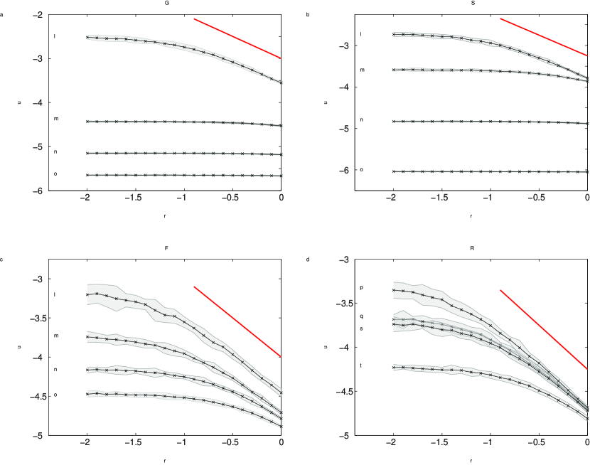
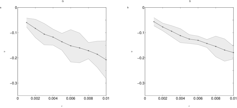
We remark that in Figure 1, an scaling only applies to a parameter regime sufficiently far from . We interpret this as the regime in which linearization is valid, and infer that nonlinearity is important near . For both the GL and SH equations, it is expected that these two regimes (of linear and nonlinear behavior) are separated by a narrow transition regime of weakly nonlinear behavior, and it can be shown that this weakly nonlinear regime occurs near , where is the amplitude of the critical Fourier mode [22, 21]. Since in this stochastic setting is directly influenced by the the magnitude of the input noise , we expect that occurs at a smaller value for smaller values of , i.e., as , . We confirm this numerically using simulations of the GL and SH equations, taking , , and . In each set of simulations using a constant value of and over a range of , a point is computed where the critical Fourier mode variance first appears to diverge from the scaling law. These points are plotted as functions of in Figure 2, and it appears, as predicted, that as . Hence, the influence of nonlinearity in the GL and SH SPDEs on the warning signs presented in earlier sections diminishes as .
4.2 Other early-warning signs
Here, we describe other generic early-warning signs that have been proposed for spatio-temporal processes and explore them numerically in the SH SPDE. One natural measure to consider is the variance of , which we compute by averaging spatial variance over time:
| (27) |
We note that is approximately equal to the temporal variance averaged over space,
since as long as are sufficiently large. This example suggests how temporal and spatial variance can be related as early-warning signs in general. In analogy to the univariate early-warning sign, we also compute the autocorrelation as a function of time lag , averaged over space:
| (28) |
where . Another measure not typically considered as an early-warning sign is the supremum of the process over all space and time:
| (29) |
This measure generally depends on the end time, , since large deviations occur as rare events. We may expect (as with white noise) that as , but the rate at which certain maxima or minima of the stochastic process diverge as may be different for different values of .
To explore the relationship between these measures and the factors of domain size, noise type, and noise correlation length, we numerically simulated the SH SPDE for values of . For some of these simulations, alternative domain sizes of and are considered. For other simulations, is generated as either space-time white noise or noise that is colored in space, i.e. . The form was chosen, with representing a short correlation length and representing an intermediate correlation length for domain size . Details about the generation of space-colored noise are described in A.1. Numerical parameter values and simulation details are otherwise as previously described.
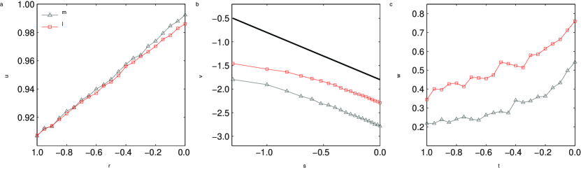
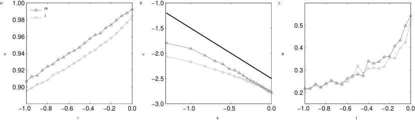
Figure 3 compares the effect of white noise and spatially-colored noise on the scaling of (28), (27), and (29) with . The domain size and the noise correlation function were used. For both types of noise, all three measures appear to scale with in a similar way. We observe a clear monotonic increase in lag- temporal autocorrelation as . We also see a near scaling of the spatial variance when is sufficiently far from . This reflects the dominant effect of critical mode variance on overall spatial variance (from Figure 1, we observe the variance of non-critical modes is negligible for space-time white noise). Suprema clearly increase as , as well. The magnitude of variation, as expressed by and , is greater for spatially colored noise, which we conjecture is related to the distribution of energy in the power spectrum of the noise. The energy of space-time white noise is distributed evenly across all non-zero Fourier modes, while energy is concentrated around the SH critical mode () for noise with the spatial correlation function we consider here.
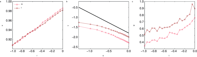
A similar comparison for two different colored noise correlation lengths is shown in Figure 4. Again, the domain size was used, and the noise correlation functions (short correlation length) and (intermediate correlation length) were considered. For both correlation lengths, all three measures once again appear to scale with in a similar way. Additionally, we observe that the magnitude of variation is greater for the intermediate correlation length simulations. As before, we conjecture that the reason for this can be found in the noise power spectrum. The intermediate correlation noise has more energy in the critical SH Fourier mode than the short correlation noise in this case.
Finally, Figure 5 shows the effect of domain size on , , and . Space-time white noise was used for simulations with domain sizes and . Here, we observe that domain size has an effect on the autocorrelation signal. Specifically, for is less than for for all values of . Also, we see that the larger domain size loses the overall scaling in spatial variance, instead growing more slowly as . This could have been anticipated from the observed scaling of non-critical modes in Figure 1. We note that suprema appear to scale in the same way for both domain sizes, which suggests a potential domain size invariant early-warning sign.
5 Conclusions & outlook
In this paper, we have begun to develop elements of a mathematical theory for early-warning signs in pattern-forming SPDEs, specifically in the homogeneous regime before a first bifurcation point. In particular, we gave an analytical treatment of the scaling laws for covariance operators of the linearized SPDE problem. This analysis included the linearized GL and SH equations, which we investigated numerically in the second part of this work. In the numerical simulations, we focused on the influence of distance to bifurcation, noise strength, noise color and domain size.
Although we believe that our work provides a basis for the study of early-warning signs in SPDEs, many open problems remain. We have attempted to collect several references from different fields as additional starting points for future research. There are many natural mathematical problems that seem to be of particular interest in spatial early-warning sign applications. For example, given a particular pattern-forming system, can we give precise estimates for different regime sizes and early-warning sign scaling laws in these regimes for the covariance operators (and other statistical measures) of the linearized problem in comparison to the full nonlinear problem? What role do amplitude equations for SPDEs play in this context? How can we classify which models display warning signs for spatio-temporal patterns? From these questions, it is clear that there are many mathematical challenges that remain to be addressed in order to quantify the the dynamics of stochastic systems operating near instability.
Acknowledgements: KG thanks Mary Silber for useful conversations throughout the duration of this project, and gratefully acknowledges support from the NSF Math and Climate Research Network (DMS-0940262). CK thanks the Austrian Academy of Sciences (ÖAW) for support via an APART fellowship and acknowledges the European Commission (EC/REA) for support by a Marie-Curie International Re-integration Grant. CK also thanks Dirk Blömker for inspiring discussion at the workshop “Infinite-Dimensional Stochastic Systems: Theory and Applications” (Wittenberg, January 2014). We also thank two anonymous referees for very insightful comments, which helped to improve the manuscript.
Appendix A Numerical methods
A.1 Generation of colored noise in space
The following procedure for generating a noise field that is colored in space and white in time is described in [32]. For with , it can be shown that if
and the Fourier transform of is finite, then
where hats denote a function transformed to Fourier -space:
This decoupling of modes in Fourier space can be exploited to construct :
| (30) |
where are complex random variables such that , with real and imaginary parts drawn from the normal distribution with mean 0 and . From here, (30) can be transformed back into real space to obtain . The practical implementation of this approach in MATLAB is performed approximately for using the Fast Fourier Transform (FFT):
x=linspace(0, L, N+1); x = x(1:N); %Spatial domain
Cspa=exp(-((x-L/2).^2)); %Example spatial correlation function
Ck=fft(Cspa); %Fast Fourier transform of the correlation function

%Generate anticorrelated noise field in Fourier space
randNums=randn(1,N);
alphak=sqrt(N)*[randNums(1), sqrt(1/2)*(randNums(2:N/2)+...
    1i*randNums(N/2+1:end-1)), randNums(N),...
    sqrt(1/2)*(fliplr(randNums(2:N/2)-1i*randNums(N/2+1:end-1)))];
ΨΨ
xik=alphak.*sqrt(Ck);
xi=ifft(xik); %Invert Fourier transform
A.2 Finite difference solution of SPDE
A finite difference method in space is used to discretize the SPDE in space to obtain SODEs as described below. Then an implicit Euler-Maruyama scheme is used to solve (5) with . The SODE scheme is described in [48, 41]. Space and time are discretized as and , and the discrete solution is denoted . The simulations generated for this paper used numerical parameter values , , , and . Initial conditions were taken to be uniformly random in space and were drawn from the interval . The spatial derivatives of (5) are discretized using central differencing operators, i.e.
This discretization results in a system of coupled SODEs,
| (31) |
where . For instance, when is defined as in (2), is
To satisfy periodic boundary conditions, . The solution of (31) at is implicitly defined by the update equation
| (32) |
Newton’s method is used to iteratively solve (32). Explicitly, (32) is written
Then the Newton iteration formula (on the index ) for is given by
where is the Jacobian matrix of with respect to , evaluated at , and . The iteration terminates when is less than a prescribed tolerance value.
References
- [1] G. Agez, M.G. Clerc, E. Louvergneaux, and R.G. Rojas. Bifurcations of emerging patterns in the presence of additive noise. Phys. Rev. E, 87(4):042919, 2013.
- [2] P. Ashwin, S. Wieczorek, R. Vitolo, and P. Cox. Tipping points in open systems: bifurcation, noise-induced and rate-dependent examples in the climate system. Phil. Trans. R. Soc. A, 370:1166–1184, 2012.
- [3] A. Becker and L. Kramer. Linear stability analysis for bifurcations in spatially extended systems with fluctuating control parameter. Phys. Rev. Lett., 73(7):955–958, 1994.
- [4] N. Berglund and B. Gentz. Pathwise description of dynamic pitchfork bifurcations with additive noise. Probab. Theory Related Fields, 3:341–388, 2002.
- [5] N. Berglund and B. Gentz. Noise-Induced Phenomena in Slow-Fast Dynamical Systems. Springer, 2006.
- [6] N. Berglund, B. Gentz, and C. Kuehn. Hunting French ducks in a noisy environment. J. Differential Equat., 252(9):4786–4841, 2012.
- [7] J. Berwald and M. Gidea. Critical transitions in a model of a genetic regulatory system. arXiv:1309.7919, pages 1–19, 2013.
- [8] D. Blömker. Amplitude equations for locally cubic nonautonomous nonlinearities. SIAM J. Appl. Dyn. Syst., 2(3):464–486, 2003.
- [9] D. Blömker. Amplitude Equations for Stochastic Partial Differential Equations. World Scientific, 2007.
- [10] D. Blömker, M. Hairer, and G.A. Pavliotis. Modulation equation for SPDEs on large domains. Comm. Math. Phys., 258:479–512, 2005.
- [11] D. Blömker and W.W. Mohammed. Amplitude equations for SPDEs with cubic nonlinearities. Stochastics, 85(2):181–215, 2013.
- [12] C. Boettinger and A. Hastings. Quantifying limits to detection of early warning for critical transitions. J. R. Soc. Interface, 9(75):2527–2539, 2012.
- [13] Z. Brzezniak and S. Peszat. Space-time continuous solutions to SPDEs driven by a homogeneous Wiener process. Studia Math., 137:261–299, 1999.
- [14] J. Burke and E. Knobloch. Localized states in the generalized Swift-Hohenberg equation. Phys. Rev. E, 73:056211, 2006.
- [15] S.R. Carpenter and W.A. Brock. Rising variance: a leading indicator of ecological transition. Ecology Letters, 9:311–318, 2006.
- [16] O. Carrillo, M.A. Santos, J. Garcia-Ojalvo, and J.M. Sancho. Spatial coherence resonance near pattern-forming instabilities. Europhys. Lett., 65(4):452, 2004.
- [17] A.A. Cimatoribus, S.S. Drijfhout, V. Livina, and G. van der Schrier. Dansgaard-Oeschger events: tipping points in the climate system. Climate of the Past Discussion, 8(5):4269–4294, 2012.
- [18] P. Collet and J.P. Eckmann. Instabilities and Fronts in Extended Systems. Princeton University Press, 1990.
- [19] P. Collet and J.P. Eckmann. The time dependent amplitude equation for the Swift-Hohenberg problem. Comm. Math. Phys., 132(1):139–153, 1990.
- [20] E. Cotilla-Sanchez, P. Hines, and C.M. Danforth. Predicting critical transitions from time series synchrophasor data. IEEE Trans. Smart Grid, 3(4):1832–1840, 2012.
- [21] M. Cross and H. Greenside, editors. Pattern Formation and Dynamics in Nonequilibrium Systems. CUP, 2009.
- [22] M.C. Cross and P.C. Hohenberg. Pattern formation outside of equilibrium. Rev. Mod. Phys., 65(3):851–1112, 1993.
- [23] V. Dakos, S.R. Carpenter, W.A. Brock, A.M. Ellison, V. Guttal, A.R. Ives, S. Kéfi, V. Livina, D.A. Seekell, E.H. van Nes, and M. Scheffer. Methods for detecting early warnings of critical transitions in time series illustrated using simulated ecological data. PLoS One, 7(7):e41010, 2012.
- [24] V. Dakos, S. Kéfi, M. Rietkerk, E.H. van Nes, and M. Scheffer. Slowing down in spatially patterned systems at the brink of collapse. Am. Nat., 177(6):153–166, 2011.
- [25] V. Dakos, M. Scheffer, E.H. van Nes, V. Brovkin, V. Petoukhov, and H. Held. Slowing down as an early warning signal for abrupt climate change. Proc. Natl. Acad. Sci. USA, 105(38):14308–14312, 2008.
- [26] V. Dakos, E.H. van Nes, R. Donangelo, H. Fort, and M. Scheffer. Spatial correlation as leading indicator of catastropic shifts. Theor. Ecol., 3(3):163–174, 2009.
- [27] P.D. Ditlevsen and S.J. Johnsen. Tipping points: early warning and wishful thinking. Geophys. Res. Lett., 37:19703, 2010.
- [28] R. Donangelo, H. Fort, V. Dakos, M. Scheffer, and E.H. Van Nes. Early warnings for catastrophic shifts in ecosystems: comparison between spatial and temporal indicators. Int. J. Bif. Chaos, 20(2):315–321, 2010.
- [29] K.R. Elder, J. Vinals, and M. Grant. Ordering dynamics in the two-dimensional stochastic Swift-Hohenberg equation. Phys. Rev. Lett., 68(20):3024–3027, 1992.
- [30] L.C. Evans. Partial Differential Equations. AMS, 2002.
- [31] A. García-Ojalvo, A. Hernández-Machado, and J.M. Sancho. Effects of external noise on the Swift-Hohenberg equation. Phys. Rev. Lett., 71(10):1542–1545, 1993.
- [32] J. Garcia-Ojalvo and J. Sancho. Noise in Spatially Extended Systems. Springer, 1999.
- [33] D.I. Goldman, J.B. Swift, and H.L. Swinney. Noise, coherent fluctuations, and the onset of order in an oscillated granular fluid. Phys. Rev. Lett., 92(17):174302, 2004.
- [34] B. Goldys and J.M.A.M. Van Neerven. Transition semigroups of Banach space-valued Ornstein-Uhlenbeck processes. Acta Applicandae Mathematica, 76:283–330, 2003.
- [35] M. Gubinelli and S. Tindel. Rough evolution equations. Ann. Probab., 38:1–75, 2010.
- [36] J. Guckenheimer and P. Holmes. Nonlinear Oscillations, Dynamical Systems, and Bifurcations of Vector Fields. Springer, New York, NY, 1983.
- [37] V. Guttal and C. Jayaprakash. Spatial variance and spatial skewness: leading indicators of regime shifts in spatial ecological systems. Theor. Ecol., 2:3–12, 2009.
- [38] M. Hairer. An Introduction to Stochastic Partial Differential Equations. Lecture Notes, 2009. http://www.hairer.org/notes/SPDEs.pdf.
- [39] H. Held and T. Kleinen. Detection of climate system bifurcations by degenerate fingerprinting. Geophys. Res. Lett., 31:L23207, 2004.
- [40] E. Hernández-Garcia, M. San Miguel, and R. Toral. Noise and pattern selection in the one-dimensional Swift-Hohenberg equation. Physica D, 61(1):159–165, 1992.
- [41] D.J. Higham. An algorithmic introduction to numerical simulation of stochastic differential equations. SIAM Review, 43(3):525–546, 2001.
- [42] P.C. Hohenberg and J.B. Swift. Effects of additive noise at the onset of Rayleigh-Bénard convection. Phys. Rev. A, 46(8):4773–4785, 1992.
- [43] R. Hoyle. Pattern Formation: An Introduction to Methods. Cambridge University Press, 2006.
- [44] A. Hutt, A. Longtin, and L. Schimansky-Geier. Additive global noise delays turing bifurcations. Phys. Rev. Lett., 98(23):230601, 2007.
- [45] A. Hutt, A. Longtin, and L. Schimansky-Geier. Additive noise-induced Turing transitions in spatial systems with application to neural fields and the Swift–Hohenberg equation. Physica D, 237(6):755–773, 2008.
- [46] S. Kéfi, M. Rietkerk, C.L. Alados, Y. Peyo, V.P. Papanastasis, A. ElAich, and P.C. de Ruiter. Spatial vegetation patterns and imminent desertification in Mediterranean arid ecosystems. Nature, 449:213–217, 2007.
- [47] E. Kirkinis. The validity of modulation equations for extended systems with cubic nonlinearities. Proc. R. Soc. Edinburgh A, 122(1):85–91, 1992.
- [48] P.E. Kloeden and E. Platen. Numerical Solution of Stochastic Differential Equations. Springer, 2010.
- [49] C. Kuehn. A mathematical framework for critical transitions: bifurcations, fast-slow systems and stochastic dynamics. Physica D, 240(12):1020–1035, 2011.
- [50] C. Kuehn. Deterministic continuation of stochastic metastable equilibria via Lyapunov equations and ellipsoids. SIAM J. Sci. Comp., 34(3):A1635–A1658, 2012.
- [51] C. Kuehn. A mathematical framework for critical transitions: normal forms, variance and applications. J. Nonlinear Sci., 23(3):457–510, 2013.
- [52] C. Kuehn. Warning signs for wave speed transitions of noisy Fisher-KPP invasion fronts. Theor. Ecol., 6(3):295–308, 2013.
- [53] C. Kuehn. Numerical continuation and SPDE stability for the 2D cubic-quintic Allen-Cahn equation. arXiv:1408.4000, pages 1–26, 2014.
- [54] C. Kuehn, E.A. Martens, and D. Romero. Critical transitions in social network activity. J. Complex Networks, 2(2):141–152, 2014.
- [55] C. Kuehn, G. Zschaler, and T. Gross. Early warning signs for saddle-escape transitions in complex networks. arXiv:1401.7125, pages 1–18, 2014.
- [56] F. Kwasniok. Analysis and modelling of glacial climate transitions using simple dynamical systems. Phil. Trans. R. Soc. A, 371(1991):20110472, 2013.
- [57] S.J. Lade and T. Gross. Early warning signals for critical transitions: a generalized modeling approach. PLoS Comp. Biol., 8:e1002360–6, 2012.
- [58] T.M. Lenton. Early warning of climate tipping points. Nature Climate Change, 1(4):201–209, 2011.
- [59] T.M. Lenton, H. Held, E. Kriegler, J.W. Hall, W. Lucht, S. Rahmstorf, and H.J. Schellnhuber. Tipping elements in the Earth’s climate system. Proc. Natl. Acad. Sci. USA, 105(6):1786–1793, 2008.
- [60] T.M. Lenton, V.N. Livina, V. Dakos, E.H. van Nes, and M. Scheffer. Early warning of climate tipping points from critical slowing down: comparing methods to improve robustness. Phil. Trans. R. Soc. A, 370:1185–1204, 2012.
- [61] J. Lim and B.I. Epureanu. Forecasting a class of bifurcations: theory and experiment. Phys. Rev. E, 83(1):016203, 2011.
- [62] V.N. Livina and T.M. Lenton. A modified method for detecing incipient bifurcations in a dynamical system. Geophysical Research Letters, 34:L03712, 2007.
- [63] G. Lythe. Stochastic PDEs: Domain formation in dynamic transitions. Anales des Física, Monografías RSEF, 4:55–63, 1998. see also arxiv:cond-mat/9808242v1.
- [64] G. Lythe and S. Habib. Stochastic PDEs: convergence to continuum? Comput. Phys. Commun., 142:29–35, 2001.
- [65] C. Meisel and C. Kuehn. On spatial and temporal multilevel dynamics and scaling effects in epileptic seizures. PLoS ONE, 7(2):e30371, 2012.
- [66] W.W. Mohammed, D. Blömker, and K. Klepel. Modulation equation for stochastic Swift–Hohenberg equation. SIAM J. Math. Anal., 45(1):14–30, 2013.
- [67] B. Øksendal. Stochastic Differential Equations. Springer, Berlin Heidelberg, Germany, 5th edition, 2003.
- [68] S.M. O’Regan and J.M. Drake. Theory of early warning signals of disease emergence and leading indicators of elimination. Theor. Ecol., 6(3):333–357, 2013.
- [69] P.-M-Lam and D. Bagayoko. Spatiotemporal correlation of colored noise. Phys. Rev. E, 48(5):3267–3270, 1993.
- [70] A. Pazy. Semigroups of Linear Operators and Applications to Partial Differential Equations. Springer, New York, 1983.
- [71] S. Peszat and J. Zabczyk. Stochastic evolution equations with a spatially homogeneous Wiener process. Stochastic Processes Appl., 72:187–204, 1997.
- [72] G. Da Prato. Kolmogorov Equations for Stochastic PDEs. Birkhäuser, 2004.
- [73] G. Da Prato and J. Zabczyk. Stochastic Equations in Infinite Dimensions. Cambridge University Press, 1992.
- [74] M. Scheffer, J. Bascompte, W.A. Brock, V. Brovkhin, S.R. Carpenter, V. Dakos, H. Held, E.H. van Nes, M. Rietkerk, and G. Sugihara. Early-warning signals for critical transitions. Nature, 461:53–59, 2009.
- [75] M. Scheffer and S.R. Carpenter. Catastrophic regime shifts in ecosystems: linking theory to observation. TRENDS in Ecol. and Evol., 18(12):648–656, 2003.
- [76] M. Scheffer, S.R. Carpenter, T.M. Lenton, J. Bascompte, W. Brock, V. Dakos, J. van de Koppel, I.A. van de Leemput, S.A. Levin, E.H. van Nes, M. Pascual, and J. Vandermeer. Anticipating critical transitions. Science, 338:344–348, 2012.
- [77] D.A. Seekell, S.R. Carpenter, and M.L. Pace. Conditional heteroscedasticity as a leading indicator of ecological regime shifts. Am. Nat., 178:442–451, 2011.
- [78] S.H. Strogatz. Nonlinear Dynamics and Chaos. Westview Press, 2000.
- [79] J. Swift and P.C. Hohenberg. Hydrodynamic fluctuations at the convective instability. Phys. Rev. A, 15(1):319–328, 1977.
- [80] J.M.T. Thompson and J. Sieber. Climate tipping as a noisy bifurcation: a predictive technique. IMA J. Appl. Math., 76(1):27–46, 2011.
- [81] A. van Harten. On the validity of the Ginzburg-Landau equation. J. Nonlinear Sci., 1(4):397–422, 1991.
- [82] E.H. van Nes and M. Scheffer. Slow recovery from perturbations as generic indicator of a nearby catastrophic shift. Am. Nat., 169(6):738–747, 2007.
- [83] J.G. Venegas, T. Winkler, G. Musch, M.F. Vidal Melo, D. Layfield, N. Tgavalekos, A.J. Fischman, R.J. Callahan, G. Bellani, and R.S. Harris. Self-organized patchiness in asthma as a prelude to catastrophic shifts. Nature, 434:777–782, 2005.
- [84] J.M.G. Vilar and J.M. Rubi. Spatiotemporal stochastic resonance in the Swift-Hohenberg equation. Phys. Rev. Lett., 78(15):2886–2889, 1997.
- [85] J. Vinals, E. Hernández-Garcia, M. San Miguel, and R. Toral. Numerical study of the dynamical aspects of pattern selection in the stochastic Swift-Hohenberg equation in one dimension. Phys. Rev. A, 44(2):1123–1133, 1991.
- [86] J.B. Walsh. An introduction to stochastic partial differential equations. In École d’été de probabilités de Saint-Flour, XIV - 1984, volume 1180 of Lecture Notes in Math., pages 265–439. Springer, 1986.