Non-uniform Feature Sampling for Decision Tree Ensembles
Abstract
We study the effectiveness of non-uniform randomized feature selection in decision tree classification. We experimentally evaluate two feature selection methodologies, based on information extracted from the provided dataset: leverage scores-based and norm-based feature selection. Experimental evaluation of the proposed feature selection techniques indicate that such approaches might be more effective compared to naive uniform feature selection and moreover having comparable performance to the random forest algorithm [3].
1 Introduction
Living in the era of Big Data, massive amount of information is now publicly available, aggrandizing our expectations for new developments, both in well-established and contemporary scientific tasks. However, this ever increasing data often contradicts with the principle of parsimony: in a high-dimensional feature space the proper selection of features, that results in succinct descriptions of the problem, cannot be easily derived. This fact jeopardizing the interpretability of the solution. This curse of dimensionality can also pose difficulties with respect to the qualitative performance of methods, imperilling their accuracy as well as their robustness in the case of noise and outlier presence.
An important application that suffers from this difficulty is classification. An abstract description for the case of binary classification is given below: Binary Classification Problem: Assume
be a collection of supervised train feature vectors with corresponding labels . Given , we want to learn a classifier such that, for an unsupervised input , computes labels on the elements of with the lowest possible classification error. Several cases have been reported in the literature where classification using the over-complete set of features (i.e., without proper selection or pre-processing) can be as poor as random guessing, due to noise accumulation in the high-dimensional feature space [10].111The authors in [10] demonstrate further that almost all linear discriminants can perform as poorly as the random guessing. Wherefore, irrelevant or redundant information “interfere” with useful one and its removal could gain in classification. Fortunately, common wisdom indicates that, in practice only a few features are important for classification and thus such removal is applicable [1]; e.g., in DNA data [30, 11], only a few genes are influential in a gene sequence expression. Moreover, an excessive number of attributes usually results in prohibitive running times and storage requirements during training for real-time applications; in memory-limited cases, further post-processing is required [20].
In stark contrast, training a well-behaved individual classifier with a predetermined and fixed subset of features over a restricted train dataset is a difficult task; it often creates overfitting issues, where the loss of generalization is observed on incoming new data. To overcome this difficulty, recent developments [17, 16, 15], based on [19], have proposed the systematic construction of classifiers: randomly and independently selected subsets of features are used per learner and the final decision is taken as a majority (averaging) rule over the collection of learners for the given data; such structures are generally known as classifier ensembles [7].
However, a naive selection of features might still doubt the practicality of classifier ensembles in such settings: the random selection might lead to extremely “weak” learners, increasing drastically the number of ensemble components required for a desired classification error. Moreover, the authors of [18] highlight the exponentially increasing space-complexity of tree-based ensembles to achieve a given accuracy; thus, more sophisticated selection procedures might lead to less expensive constructions.
To this end, a compromise between these two extremes is imperative in practice: by judiciously selecting a subset of significant attributes, allowing randomness during the selection, one can achieve acceptable classification accuracy and desired generalization attributes with low space complexity.
Our contributions: In this context, sophisticated dimensionality reduction techniques might play a crucial role. Instead of selecting features uniformly at random, we utilize linear algebraic techniques to “bias” the selection procedure. Based on the work [9, 22, 28], we use matrix-based information scores to define a non-uniform probability distribution that favors more dominant features.
Empirical results show an overall improved classification capability using our approach, as compared to classic state-of-the-art schemes for a given training time period.
2 Related Work
As already mentioned above, a classical technique in classification focuses on the idea of ensemble classifiers: by combining a set of “weak” learners that approximate the training data, one could obtain a “strong” classifier, i.e., a classifier with better generalization performance (see e.g., [13]). Based on this approach, one can generate several “weak” learners by applying one or combination of the following designs:
-
Training data subsampling and reweighting: each classifier is trained over a subset of the training samples; then, the sample selection scheme is re-weighted, based on the classification error in the previous iteration—e.g., see the celebrated Boosting technique [29] and references therein.222To use such approach, one assumes many passes over the data.
-
Linear combination of features under random low-dimensional embeddings, where each learner uses the whole spectrum of features, trasformed by random linear mappings.
There are several works in the literature where combinations of the above designs are used in practice—e.g., Random Forests with feature selection and data subsampling [3].
In [1, 16, 8, 12], the authors consider case where the random model is proposed: to train a “weak” learner, each feature is selected uniformly at random, ignoring any prior information. While such strategy is maximally “unbiased” and easy to implement, it might lead to lower classification accuracy when a small number of features is selected each time or to higher complexity, due to the larger amount of classifiers required for a given accuracy level. In [17, 12], the authors further extend this strategy to node optimization for tree-based ensembles: at every level of each decision tree in the ensemble, the splitting decision rule over each node is derived using a random subset of features; in this work, our proposal does not consider this case and we leave it as a future research direction.
In this context, [3, 12] show that randomization yields strict improvements over simple deterministic selection heuristics.333A non-exhaustive list of such rules in the case of tree-based classifiers includes Gain ratio and Gini index, designed to result into simple models for classification. While simplicity helps, randomization is particularly useful in “adversarial” settings where “bad” features are present. [3] states the accuracy of RFs is insensitive to randomness in practice, see also [12]. However, subsequent developments on tree-based classifiers do not espouse this virtue. The author in [26] proposes the ReliefF feature evaluation metric: the significance of each attribute is inversely proportional to what extent its values separate similar observations into different classes; details of this algorithm are provided in [27]. [4] proposes the Probabilistic RFs where feature selection procedure is further linearly transformed with linear kernels. Such works amplify the suspicion that one can achieve more by applying sophisticated selection strategies rather than the blind randomization model.
In this paper, we attempt to raise this suspicion even more: we study several matrix-based sampling measures in order to signify important features in the selection procedure for higher classification accuracy.
3 Problem setting
Throughout this paper, we use decision trees as “weak” learners; an illustrative example for a binary decision tree is given in Figure 1. These structures have inherent interpretation capabilities due to the explicit decision rules on the splitting nodes, are non-parametric, easy to implement and extremely fast to train, as compared to other classifiers. A non-exhaustive list of alternatives include linear classifiers [31, 21], Support Vector machines [6, 14], Neural Networks [32], etc; we conjecture that our proposed feature selection scheme can be easily applied to these cases and we leave this research direction for future work.
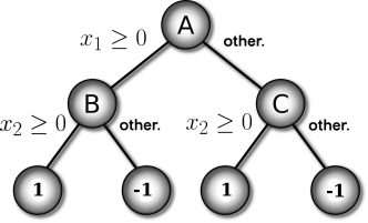
In the realm of random decision tree ensembles, we generate a set of decision trees, built on a subset of the initial feature set. We construct the ensembles as follows: for each tree, we sample non-uniformly and independently at random a set of features. Then, we train a decision tree classifier in its entirety (with a deterministic splitting criterion), restricted on these features.
It is important to notice that the above randomized procedure is quite different than Breiman’s random forest algorithm (RFs) [3, 17]. In a parameter free implementation of RFs without bagging, each tree of the forest utilizes randomness in the splitting process of its construction. Conventional wisdom indicates that, at each node during the tree growing process, an uniformly random (and possibly different) sample of features is utilized.
4 Our approach in a nutshell
To describe the main ideas of our approach, assume that we represent the training dataset of objects with features as an real444We implicitly assume that features are real-valued. matrix . We propose the LEverage ScoreS (LESS) tree ensemble algorithm, a two-phase classifier construction, as reported in Algorithm 1. Let denote a probability distribution over the set of features that signifies the importance of features over . In the first phase, we compute , based on ideas described in Section 5. Next, we “feed” into the second phase of our approach where: we select features according to and, based on these features, we generate decision trees.
Finally, the collection of these decision trees is gathered and a standard majority voting scheme is applied to derive the predicted labelling of the model. Namely, given a set of decision trees and an unlabelled example, the algorithm returns as its predicted label the most frequent label over all the decision trees.
Several remarks can be highlighted about the above algorithm. First, each decision tree is constructed on only a subset of features of size (usually is between and ); hence, as we show in Section 6, Algorithm 1 has computational advantages over models that compute the best split over the whole feature set. Along the same lines, the resulting collection of trees are more interpretable than RFs since each tree depends only on a small set of features. Last, the random process described in Algorithm 1 is simpler than the random forest algorithm [3] and hence might be amenable to theoretical justification in the future.
5 Feature Selection Schemes
Exploiting the full spectrum of features creates a tradeoff between interpretability and predictive accuracy. Thus, an important step to process such large-scale data is to construct an “importance score” for each column of to denote the influence of the corresponding feature. Given such measure, we can then sample a predefined number of features for each decision tree, based on these scores.
In this section, we describe three subsampling techniques for feature selection: uniform sampling, column squared-norm based sampling and, leverage scores-based sampling [9] (to be defined shortly). Uniform sampling: each feature is selected with equal probability. Both strategies, where features are selected with or without replacement, have been tested; cf., [16, 17]. We use this policy as the baseline performance in our experiments. Norm-based sampling: Recent developments on geometric functional analysis have dictated that squared norm subsampling can approximate well large datasets incurring small spectral norm [28]. Namely, in our setting sampling the i-th feature with probability proportional to where is the i-th column of and denote the Euclidean norm. Statistical leverage scores sampling: The goal of statistical leverage scores is to construct a judiciously-chosen nonuniform importance sampling distribution over the set of columns, based on factorizations of , according to the following definition:
Definition 1 (Statistical leverage scores [5, 9])
Let be a data matrix with objects and features with for . Moreover, let be its Singular Value Decomposition (SVD) where contains the set of right singular column vectors. The normalized statistical leverage scores over the set of columns of are defined as:
| (1) |
where denotes the -th entry of the -th right singular vector.
We highlight that, while sampling schemes and are slower than the simple uniform sampling, both result into generally higher classification accuracy for given sampling volume as we show in Section 6. Moreover, strategy can be well-approximated using fast randomized algorithms [22]. We note that leverage scores converge to uniform sampling when the coherence of the data matrix is small and scheme turns to be the optimal; thus, scheme can be considered as a more generic selection strategy that includes as a special case.
6 Experiments
In this section, we experimentally compare Algorithm 1 with two variants of Algorithm 1: the case where Step 4 is replaced with uniform/norm-based feature sampling and the classical Breiman’s RFs algorithm [3]. Here, we highlight a subtle distinction between the RFs algorithm and all other algorithms under comparison. During the tree construction, RFs utilizes randomness for deciding the next split. Namely, at each node (assuming an additional split has been decided to be made), RFs selects features uniformly at random on which the best split is selected. Therefore, one expects each resulting tree to possibly depend on all features as opposed to Algorithm 1 that depends on only features.
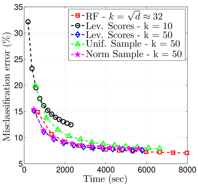
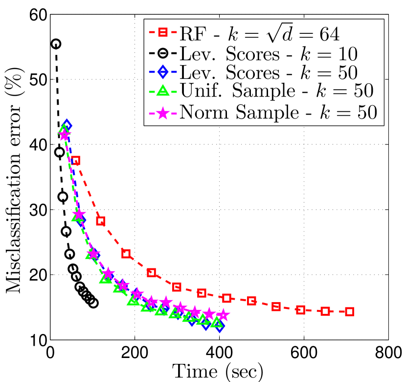
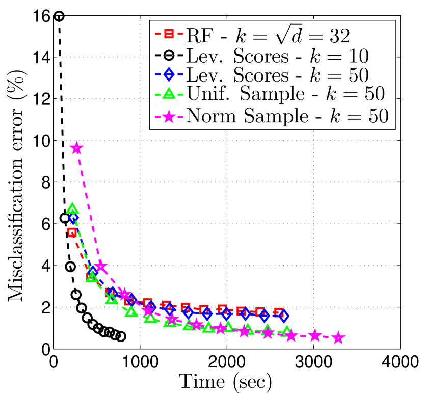
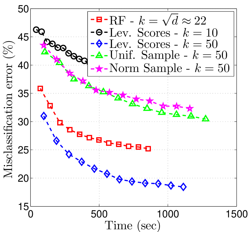
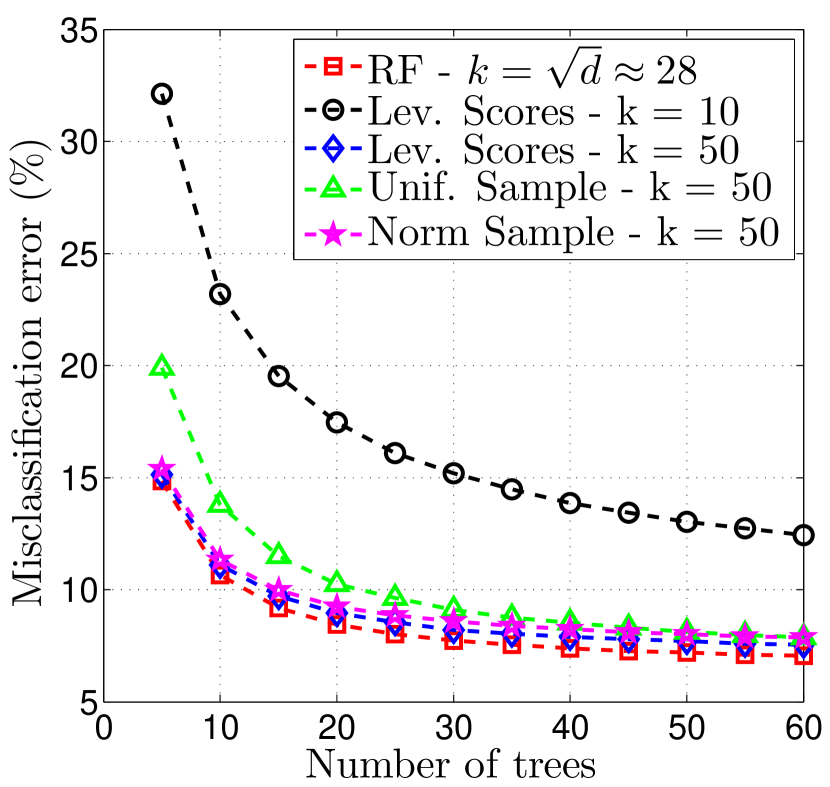
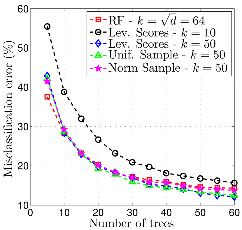
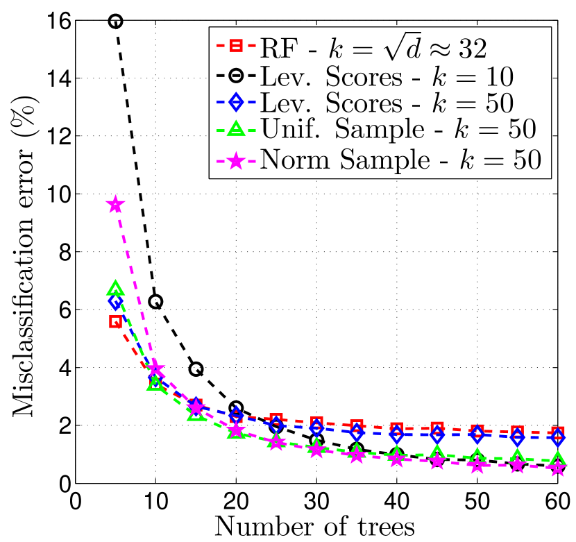
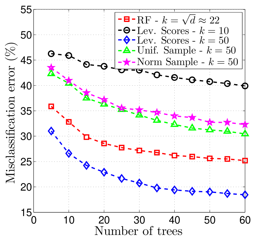
Datasets: For the real-world datasets we used four publicly available555Most of the datasets used here are available under UCI’s machine learning repository [2]. datasets that we denote by MNIST, ORL, PIE and MADELON. The MNIST dataset of handwritten digits has a training set of 60,000 examples, and a test set of 10,000 examples [2] (a sample of training examples and test examples is used here). ORL contains ten different images each of distinct subjects [24]. There are 400 different objects in total, each having 4096 dimensions. PIE is a database of 41,368 images of 68 people [25]. Namely, there are in total data points with dimensions. The MADELON dataset is an artificial test case, multivariate and highly non-linear, part of the NIPS 2003 feature selection challenge. The data points of MADELON is containing features. These datasets have been selected due to their high-dimensional feature space and/or their heavily usage as benchmarks for classification. Experimental setup: To measure the impact of leverage scores on the classification performance on random decision trees, we perform a series of diverse experiments on the above datasets. In all reported results, we use the average values of 30 independent executions of its corresponding algorithm. For the LESS algorithm, we truncate the computation of SVD to rank for acceleration. We measured the performance of Algorithm 1 for various settings of and , i.e., the number of features to be sampled and the number of trees, respectively. No bagging is performed on the RFs algorithm and the default number of subsampled features is selected, i.e., . All timings were performed under MATLAB R2011b [23]. Numerical results: We report our experimental evaluations in Figure 2 and in Table 1.
| Total number of nodes for given classification accuracy | |||||
|---|---|---|---|---|---|
| RFs | Uniform | Norm | Lev. Scores | ||
| MNIST | 102066 | 125152 | 92064 | 93527 | |
| ORL | 5498 | 5568 | 5566 | 5587 | |
| MADELON | 26407 | T | T | 4003 | |
| PIE | 18198 | 20632 | 24851 | 19137 | |
In the first row of Figure 2 we depict the classification error versus the elapsed training time for a pair of train and test data. The rationale behind this plot is to demonstrate that Algorithm 1 can achieve similar or better classification error than RFs with lower computational requirements. In all cases, LESS algorithm with is superior or matches the performance of RFs. On the other hand, the performance of Algorithm 1 with is not superior in all cases. This is due to the small value of . Hence, a suggestive setting of in Algorithm 1 is in the range . However, in stark contrast with conventional wisdom, there are cases where only features, selected using leverage scores, seem to be sufficient to achieve the same or even better classification accuracy in much less training time, increasing the interpretability of the result due to the limited number of used features; e.g., see Figure 2(first row) for the cases ORL and PIE. Moreover, an increased number of features usually results in an increased processing time, with no further classification error improvement. Overall, we observe that LESS trees are at least as accurate as RF, while being less computationally expensive in practice.
The second row of Figure 2 depicts the classification accuracy versus the number of trees. We observe that Algorithm 1 with matches the performance of RFs in terms of number of trees. Moreover, in the MADELON dataset Algorithm 1 is superior to RFs, which in turn, RFs is superior to both uniform and norm based feature selection. On the other hand, Algorithm 1 with does not perform well.
We further study the space complexity of the resulting ensembles as a function of the total number of nodes needed among all trees to achieve a predefined classification error . We also set up a time threshold limit value T seconds (1 hour) per approach to achieve accuracy . Table 1 shows the reported space complexities for all test cases. As observed, both RFs and LESS trees has similar (or even better) space complexity for given . From a different perspective, in a memory-limited scenario where only a fixed number of nodes can be maintained, non-uniform feature sampling leads to equivalent, if not better, mis-classification error level, as compared to uniform feature selection and/or RFs.
7 Discussion and Future Work
In this work, we study feature selection strategies in classification, both in terms of time/space-complexity efficiency as well as of classification accuracy. Overall, results indicate that the proposed tree ensemble, based on leverage scores, might outperform the state-of-the-art RFs [3], as well as schemes where uniform weighting is applied. We observe that the proposed scheme results into low space-complexity trees for better interpretability, requires overall less training time and has at least the same accuracy, as compared to top-notch approaches.
References
- [1] Amit, Y., and Geman, D. Shape quantization and recognition with randomized trees. Neural computation 9, 7 (1997), 1545–1588.
- [2] Bache, K., and Lichman, M. UCI Machine Learning Repository. http://archive.ics.uci.edu/ml, 2013. University of California, Irvine, School of Information and Computer Sciences.
- [3] Breiman, L. Random forests. Machine learning 45, 1 (2001), 5–32.
- [4] Breitenbach, M., Nielsen, R., and Grudic, G. Z. Probabilistic random forests: Predicting data point specific misclassification probabilities. Univ. of Colorado at Boulder, Tech. Rep. CU-CS-954-03 (2003).
- [5] Chatterjee, S., and Hadi, A. Sensitivity Analysis in Linear Regression. Wiley Series in Probability and Statistics. Wiley, 1988.
- [6] Cortes, C., and Vapnik, V. Support-vector networks. Machine learning 20, 3 (1995), 273–297.
- [7] Dasarathy, B. V., and Sheela, B. V. A composite classifier system design: concepts and methodology. Proceedings of the IEEE 67, 5 (1979), 708–713.
- [8] Dietterich, T. G. Ensemble methods in machine learning. In Multiple classifier systems. Springer, 2000, pp. 1–15.
- [9] Drineas, P., Mahoney, M. W., and Muthukrishnan, S. Relative-error cur matrix decompositions. SIAM Journal on Matrix Analysis and Applications 30, 2 (2008), 844–881.
- [10] Fan, J., and Fan, Y. High dimensional classification using features annealed independence rules. Annals of statistics 36, 6 (2008), 2605.
- [11] Fan, J., and Ren, Y. Statistical analysis of dna microarray data in cancer research. Clinical Cancer Research 12, 15 (2006), 4469–4473.
- [12] Fan, W., Wang, H., Yu, P. S., and Ma, S. Is random model better? on its accuracy and efficiency. In Data Mining, 2003. ICDM 2003. Third IEEE International Conference on (2003), IEEE, pp. 51–58.
- [13] Freund, Y., and Schapire, R. E. A decision-theoretic generalization of on-line learning and an application to boosting. J. Comput. Syst. Sci. 55, 1 (Aug. 1997), 119–139.
- [14] Gunn, S. R. Support vector machines for classification and regression. ISIS technical report 14 (1998).
- [15] Hansen, L. K., and Salamon, P. Neural network ensembles. Pattern Analysis and Machine Intelligence, IEEE Transactions on 12, 10 (1990), 993–1001.
- [16] Ho, T. K. Random decision forests. In Document Analysis and Recognition, 1995., Proceedings of the Third International Conference on (1995), vol. 1, IEEE, pp. 278–282.
- [17] Ho, T. K. The random subspace method for constructing decision forests. Pattern Analysis and Machine Intelligence, IEEE Transactions on 20, 8 (1998), 832–844.
- [18] Joly, A., Schnitzler, F., Geurts, P., and Wehenkel, L. L1-based compression of random forest models. In 20th European Symposium on Artificial Neural Networks (2012).
- [19] Kleinberg, E. Stochastic discrimination. Annals of Mathematics and Artificial intelligence 1, 1 (1990), 207–239.
- [20] Kulkarni, V. Y., and Sinha, P. K. Pruning of random forest classifiers: A survey and future directions. In Data Science & Engineering (ICDSE), 2012 International Conference on (2012), IEEE, pp. 64–68.
- [21] Liu, C., and Wechsler, H. Gabor feature based classification using the enhanced fisher linear discriminant model for face recognition. Image processing, IEEE Transactions on 11, 4 (2002), 467–476.
- [22] Mahoney, M. W., Drineas, P., Magdon-Ismail, M., and Woodruff, D. P. Fast approximation of matrix coherence and statistical leverage. In ICML (2012).
- [23] MATLAB. 7.13.0.564 (R2011b). The MathWorks Inc., Natick, Massachusetts, 2010.
- [24] The ORL Database of Faces. http://www.cl.cam.ac.uk/research/dtg/attarchive/facedatabase.html. AT&T Laborartories Cambridge, UK.
- [25] PIE Database. http://www.ri.cmu.edu/research_project_detail.html?project_id=418&menu_id=261. Carnegie Mellon University.
- [26] Robnik-Šikonja, M. Improving random forests. In Machine Learning: ECML 2004. Springer, 2004, pp. 359–370.
- [27] Robnik-Šikonja, M., and Kononenko, I. Theoretical and empirical analysis of relieff and rrelieff. Machine learning 53, 1-2 (2003), 23–69.
- [28] Rudelson, M., and Vershynin, R. Sampling from large matrices: An approach through geometric functional analysis. Journal of the ACM (JACM) 54, 4 (2007), 21.
- [29] Schapire, R. E. The boosting approach to machine learning: An overview. Lecture notes in Statistics - New York - Springer Verlag (2003), 149–172.
- [30] West, M., Blanchette, C., Dressman, H., Huang, E., Ishida, S., Spang, R., Zuzan, H., Olson, J. A., Marks, J. R., and Nevins, J. R. Predicting the clinical status of human breast cancer by using gene expression profiles. Proceedings of the National Academy of Sciences 98, 20 (2001), 11462–11467.
- [31] Witten, D. M., and Tibshirani, R. Penalized classification using fisher’s linear discriminant. Journal of the Royal Statistical Society: Series B (Statistical Methodology) 73, 5 (2011), 753–772.
- [32] Zhang, G. P. Neural networks for classification: a survey. Systems, Man, and Cybernetics, Part C: Applications and Reviews, IEEE Transactions on 30, 4 (2000), 451–462.