Utility Max-Min Fair Link Adaptation in IEEE 802.11ac Downlink Multi-User

Abstract

In this letter, we propose a novel model and corresponding algorithms to address the optimal utility max-min fair link adaptation in Downlink Multi-User (DL-MU) feature of the emerging IEEE 802.11ac WLAN standard. Herein, we first propose a simple yet accurate model to formulate the max-min fair link adaptation problem. Furthermore, this model guarantees the minimum utility gain of each receiver according to its requirements. In the second step, we show that the optimal solution of the proposed model can be obtained in polynomial time, and then the solution algorithms are proposed and analyzed. The simulation results demonstrate the significant achievement of the proposed utility-aware link adaptation approach in terms of max-min fairness and utility gain compared to utility-oblivious schemes.

I Introduction

Utility max-min (UMM) fairness has been applied in numerous applications since the initial work by Cao and Zegura [1], who attempt to find an optimal resource allocation such that the utilities of all receivers are equal. Hence, the social welfare in the network is equalized. More precisely, this can be achieved by solving the following optimization problem:

$$\mathbf{\mathbf{UMM}:}\max_{\rho_{r}^{i}}\min_{r\in R}U_{r}(\rho_{r}^{i})$$ (1)

$$s.t.\begin{cases}\sum_{r=1}^{R}p_{r}^{i}\leq P_{T}\\ \forall m_{r}^{j},\,j=1\ldots M\end{cases}$$ (2)

where $r\,(r=1,2,..R|$$R:$ the number of receivers$)$ is the receiver index, $\rho_{r}^{i}\in\left\{\rho_{r}^{1},\rho_{r}^{2},\ldots\right\}$ is defined as the $i\textrm{th}$ policy ($i=1,2,\ldots$) of all available link adaptation policies, which further determines the selected Modulation and Coding Scheme (MCS) $m_{r}^{j}$ ($j=1\ldots M$$|M:$ the number of total available MCS) and the allocated power $p_{r}^{i}$ ($p_{r}^{i}\in[0..P_{T}]\textrm{$|P_{T}:$the total available transmission power})$, and finally $U_{r}(\rho_{r}^{i})$ is the utility of receiver $r$ due to the applied policy $\rho_{r}^{i}$. Through this letter, we assume each $U_{r}$ is a positive, non-decreasing and normalized utility function of $\rho_{r}^{i}$ [2]. The max-min problem $\mathbf{\mathbf{UMM}}$, has a unique optimal solution under a critical assumption of strict high Signal to Interference and Noise Ratio (SINR) and concavity of the receiver utilities $U_{r}(\rho_{r}^{i})$. However, there are three impediments in applying the problem formulation (1). First, the concavity assumption does not hold for real-time applications such as video transmission and Voice over IP (VoIP). The utility of these applications can be approximated by a step or a sigmoid function. Moreover, the high SINR assumption is not guaranteed in WLANs. As a result, the optimization problem (1), in general, is a non-convex problem and cannot be reduced to Geometric Programming (GP). Indeed, it belongs to the class of problems known as Complementary GP that is, in general, an NP-hard or that may require a very complex algorithm to solve [3]. Second, real-time applications that need a certain amount of transmission resources to provide the minimum required satisfaction (acceptance) suffer from so called “bandwidth starvation”. Third, in applying the theoretical formulas to predict the bit rate and corresponding Frame Error Rate (FER) associated with the link adaptation policy $\rho_{r}^{i}$, there are simply too many ways in which the observed measurements and the actual performance fail to match the predictions of the theory [4]. Through this letter, it is shown that the proposed scheme efficiently addresses these three impediments.

The IEEE 802.11ac is developed by extending the air–interface techniques of the 802.11n standard. Among the offered features, the DL-MU exploits the beamforming technique to steer signal maxima on certain receivers while suppressing, or at least greatly reducing the corresponding interference over the others. The channel state information (CSI) of the target receivers needs to be known at the transmitter, and it is provided by the channel estimation module in the standard [5].

In this letter, we propose a novel, practical, and optimal link adaptation algorithm in order to achieve the max-min fair utility distribution among the receivers in the IEEE 802.11ac DL-MU.

II Proposed Model and Theoretical Explanations

We first start with devising a model to predict the FER corresponding to each selected policy $\rho_{r}^{i}$ in order to address the third aforementioned impediment. In [4], the authors propose a model, which, by using the concept of effective SNR, performs FER prediction for each choice of $\rho_{r}^{i}$. We further extend their model to include beamforming and to match the 802.11ac specification [5], as follows. In accordance with the precoding scheme applied by the transmitter, the SNR of $l$th subcarrier of the receiver $r$ (denoted by $\varsigma_{l_{r}}$), is obtained based on the available CSI at the transmitter. For instance, in the case of zero-forcing, the average SNR value of the certain subcarrier $l$ is calculated as

$$\varsigma_{l_{r}}=\frac{p_{r}^{i}\times||\mathbf{h}_{l_{r}}\mathbf{w}_{l_{r}}||^{2}}{\sigma^{2}}$$ (3)

where $||\cdot||$ is the norm of the vector, $\sigma^{2}$ is the observed noise variance at the receiver, and $\mathbf{h}_{l_{k}}=(h_{l_{r1}},h_{l_{r2}},\cdots,h_{l_{rR}})$ is the vector of channel coefficients from $R$ antennae of the transmitter to the single antenna of receiver $r$. Additionally, $\mathbf{w}_{l_{r}}$ is the unit-norm beamforming weight vector ($\mathbf{w}_{l_{r}}=(w_{l_{r1}},w_{l_{r2}},\cdots,w_{l_{rR}})$) for receiver $r$. Using (3), the BER of the wideband downlink channel $b^{m_{r}^{j}}$ for modulation of $m_{r}^{j}$ is estimated by

$$b^{m_{r}^{j}}=\frac{1}{L}\sum_{l=1}^{L}BER^{m_{r}^{j}}(\varsigma_{l_{r}})$$ (4)

where $L$ is the total number of data subcarriers, and the BER of the subcarrier $l$ is denoted by $BER^{m_{r}^{j}}(\varsigma_{l_{r}})$ as a function of the symbol SNR (here, $\varsigma_{l_{r}}$) in the narrowband channel [6]. Note that $b^{m_{r}^{j}}$ is the uncoded bit error probability for the modulation $m_{r}^{j}$. In order to obtain the upper bound of the coded FER, we use the union bound on the first-event error probability $E_{u}^{c}$. By assuming that the frame is transmitted using the convolutional code $c$, then $E_{u}^{c}=\sum_{d=d_{free}}^{\infty}a_{d}.E_{d}$, where $d_{free}$ is the free distance of the code $c$, $a_{d}$ is the total number of error events of weight $d$, and $E_{d}$ is the probability of an incorrect path of the hamming distance $d$ when it diverges from the correct path and then re-merges with it sometime later. The value of $a_{d}$ for a specific convolutional code is generated using its transfer function, and $E_{d}$ is obtained by

$$E_{d}=\begin{cases}\sum_{k=\frac{(d+1)}{2}}^{d}\binom{d}{k}\cdot(b^{m_{r}^{j}})^{k}\cdot(1-b^{m_{r}^{j}})^{d-k},\>\textrm{if d is odd}&\textrm{}\\ \\ \frac{1}{2}\cdot\binom{d}{\frac{d}{2}}\cdot(b^{m_{r}^{j}})^{\frac{d}{2}}\cdot(1-b^{m_{r}^{j}})^{\frac{d}{2}}+\\ \,\sum_{k=\frac{(d+1)}{2}}^{d}\binom{d}{k}\cdot(b^{m_{r}^{j}})^{k}\cdot(1-b^{m_{r}^{j}})^{d-k},\>\textrm{if d is even}&\textrm{}\end{cases}$$ (5)

Therefore, by applying the policy $\rho_{r}^{i}$, the predicted upper bound of FER on wideband channel (here, $FER_{eff}$) for a frame of length $L_{f}$ is

$$FER_{eff}\leq 1-(1-E_{u}^{c})^{L_{f}}$$ (6)

Using (4) and (6), we employ a method similar to [4] in order to construct the FER prediction model. In this method, based on the available CSI, for each non-overlapping range of the transmit power level $p_{r}^{\Xi}$ ($\Xi\in(p^{min},p^{max}]$$|min,max\in[1,2,...]$ and $min<max$), there exists an MCS $m_{r}^{\Theta}$ ($\Theta\in[1\ldots M]$) such that we predict $\leq FER_{eff,r}^{\Xi}$ frame error rate. Note that for each $p_{r}^{\Xi}$ (and therefore corresponding effective SNR) only one MCS $m_{r}^{\Theta}$ results in FER between $1-(\frac{1}{2})^{L_{f}}$ (useless) and $0$ (lossless). We assume that $p_{r}^{\Xi}$ has the maximum value in the range, unless stated otherwise. Subsequently, the utility value $U_{r}(\rho_{r}^{\Xi})$ associated with each tuple $\rho_{r}^{\Xi}(p_{r}^{\Xi},m_{r}^{\Theta},FER_{eff,r}^{\Xi})$ is calculated using its specific function. On-site calibration is necessary to obtain tuples of the table $\Phi_{r}(p_{r}^{\Xi},m_{r}^{\Theta},FER_{eff,r}^{\Xi})$ of length $L_{\Phi}$ (the number of tuples) for each receiver $r$.

Now, we propose a new model to address the second aforementioned impediment. First, we attempt to determine the policies that satisfy the user-defined constraints. Such constraints are crucial, especially for real-time applications that need a certain amount of transmission resources to provide the required quantity of utility. We are interested in the policy $\rho_{r}^{min}$ with the allocated power $p_{r}^{min}$ for each receiver $r$ such that the minimum utility requirement is satisfied. Accordingly, the minimization problem with the object function of $U_{r}(\rho_{r}^{\Xi})$ can be expressed as

$$\rho_{r\in R}^{min}=\min_{p_{r}^{\Xi}}(\arg\min_{\rho_{r}^{\Xi}\in\Phi_{r}}\quad U_{r}(\rho_{r}^{\Xi}))$$ (7)

$$s.t.\begin{cases}\sum_{all\,receivers}p_{r}^{\Xi}\leq P_{T}\\ p_{r}^{\Xi}\geq 0\\ \forall m_{r}^{\Theta},\,\Theta=1\ldots M\\ U_{min,r}\leq U_{r}(\rho_{r}^{\Xi})\leq 1\end{cases}$$ (8)

where $U_{min,r}$ is the user-defined minimum value of the required utility. Once the minimum required utility is granted to each receiver by (7), we attempt to maximize all utilities equally using the $\mathbf{\mathbf{UMM}}$ problem definition. Therefore, we define the utility max-min fair link adaptation problem with the object function of $O_{r}^{\Xi}(U_{r}(\rho_{r}^{\Xi}))=(U_{r}(\rho_{r}^{\Xi})-U_{min,r})$ as

$$\max_{\rho_{r}^{\Xi}\in\Phi_{r}}\min_{r\in R}(U_{r}(\rho_{r}^{\Xi})-U_{min,r})$$ (9)

$$s.t.\begin{cases}\sum_{all\,receivers}p_{r}^{\Xi}\leq P_{T}\\ p_{r}^{\Xi}\geq p_{r}^{min}\\ \forall m_{r}^{\Theta},\,\Theta=1\ldots M\\ U_{min,r}\leq U_{r}(\rho_{r}^{\Xi})\leq 1\end{cases}$$ (10)

We state the polynomial time complexity of the optimal solution to the problem (9) in the following theorem.

Theorem 1

The optimal solution of the addressed problem (9) can be obtained in $O(R\cdot L_{\Phi}\cdot\log(L_{\Phi}))$.

Proof:

If the resources can be allocated in advance, the optimal max-min fair solution is achieved by using the progressive filling algorithm [7]. In this case, the algorithm starts with all utility gains equal to 0 and increases them together at the same pace, until one or several limits are reached. It continues to increase the gains for other receivers until it is not possible to further increase any utility. If the policies are sorted descending by their utility values (gains), in the worst case it will take $O(R\cdot L_{\Phi})$ for the algorithm to accomplish this task. If this is not the case, policies can be sorted in advance, and therefore the time complexity is on the order of $O(R\cdot L_{\Phi}\cdot\log(L_{\Phi}))$.

It is worth noting that the multi-rate WLAN suffers from performance anomaly when low-rate streams occupy most of the shared channel time. According to [8], allocating same channel occupation time to the different streams solves this issue and maintains channel time fairness between the streams. In the 802.11ac DL-MU transmission, all streams have the same TXOP time which implies the channel time fairness amongst them in DL-MU transmissions. ∎

III Solution Algorithms

Algorithm 1 Finding the policy $\rho_{r}^{min}$

⬇

1 for r=1:R

2 $\Phi_{r}^{sel}$ = select array of tuples from $\Phi_{r}$

where: $\Phi_{r}^{\Xi}.U_{r}^{\Xi}\geq U_{min,r}$;

3 $\rho_{r}^{min}$ = min($\Phi_{r}^{sel}.p_{r}^{\Xi})$;

4 remove tuples with $U_{r}^{\Xi}\leq\rho_{r}^{min}.U_{r}^{\Xi}$ from $\Phi_{r}^{sel}$;

5 end

6 if $\overset{R}{\underset{r=1}{\sum}}\rho_{r}^{min}.p_{r}^{\Xi}\leq P_{T}$

7 return $\Phi_{\{r\in R\}}^{sel}$ and $\rho_{\{r\in R\}}^{min}$;

8 end

Algorithm 2 Utility max-min fair solution to the problem (9)

⬇

1 $\textrm{index}_{\Phi}$(1:R)=2; $\rho_{\{r\in R\}}^{sel}=\rho_{\{r\in R\}}^{min}$; $O_{\{r\in R\}}$=Inf(R,1);

2 for i=1:R

3 if $\Phi_{i}^{sel}.L_{\Phi}\geq 2$

4 $O_{i}$ = $\Phi_{i}^{sel}\{\textrm{index}_{\Phi}(i)\}$.$U_{i}^{\Xi}$ - $\rho_{i}^{min}$.$U_{i}^{\Xi}$;

5 end

6 end

7 while true

8 [newmin, j] = min($O_{\{r\in R\}}$);

9 if newmin == Inf

10 return $\rho_{\{r\in R\}}^{sel}$;

11 end

12 if $(\Phi_{j}^{sel}\{\textrm{index}_{\Phi}(j)\}.p_{j}^{\Xi}+\underset{r\neq j}{\sum}\rho_{r}^{sel}.p_{r}^{\Xi})\leq P_{T}$

13 $\rho_{j}^{sel}$ = $\Phi_{j}^{sel}\{\textrm{index}_{\Phi}(j)\}$;

14 $\textrm{index}_{\Phi}(j)$ = $\textrm{index}_{\Phi}(j)+1$;

15 if $\textrm{index}_{\Phi}(j)\leq\Phi_{j}^{sel}.L_{\Phi}$

16 $O_{j}$ = $\Phi_{j}^{sel}\{\textrm{index}_{\Phi}(j)\}.U_{j}^{\Xi}-\rho_{j}^{min}.U_{j}^{\Xi}$;

17 else

18 $O_{j}$ = Inf;

19 end

20 else

21 $O_{j}$ = Inf;

22 end

23 end

Theorem 1 states the existence of the polynomial-time solution algorithms to problem (9) and, therefore, the first aforementioned impediment is addressed by the proposed scheme. Here, we propose two algorithms to obtain the solutions to the problems (7) and (9). First, we propose Algorithm 1, in MATLAB pseudo-code, which provides the solution to the problem (7). Then, Algorithm 2 gives the solution to the problem (9) by exploiting the previously obtained result. In the following theorem, we state that the given solution is optimal.

Theorem 2

Algorithm 2 provides the optimal solution to the problem (9) in $O(R\cdot L_{\Phi}\cdot\log(L_{\Phi}))$.

Proof:

The progressive filling algorithm guarantees a max-min fair distribution of the utilities. We show that Algorithm 2 follows the problem formulation (9) and the progressive filling algorithm. The constraint $\sum_{\textrm{all receivers}}p_{r}^{\Xi}\leq P_{T}$ is ensured in line 12. Note that the other constraints are already met in tables $\Phi_{r}$ and $\Phi_{r}^{sel}$, which is previously defined in line 2 of Algorithm 1. Line 1 initiates the progressive filling by setting all utility gains to 0 ($\rho_{r}^{sel}=\rho_{r}^{min}\Longrightarrow O_{r}^{sel}(U_{r}(\rho_{r}^{sel})))$$=U_{r}(\rho_{r}^{sel})-U_{min,r}=0$). Lines 7-23 aim to maximize the objective function $O_{r}^{\Xi}(U_{r}(\rho_{r}^{\Xi}))$ by increasing all gains iteratively at the same pace. Lines 18 and 21 ensure the exclusion of the receivers that reach the capacity limits. The iteration (lines 7-23) continues until it is not possible to further increase the objective function (lines 9-11). ∎

Remark 1

Algorithm 1 is on the order of $O(R\cdot L_{\Phi})$ and Algorithm 2 runs in $O(R\cdot L_{\Phi}\cdot\log(L_{\Phi}))$.

IV Simulation Results

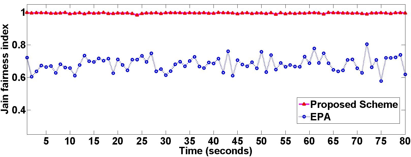
Fig. 1: Jain’s fairness index for two compared schemes: Proposed and EPA

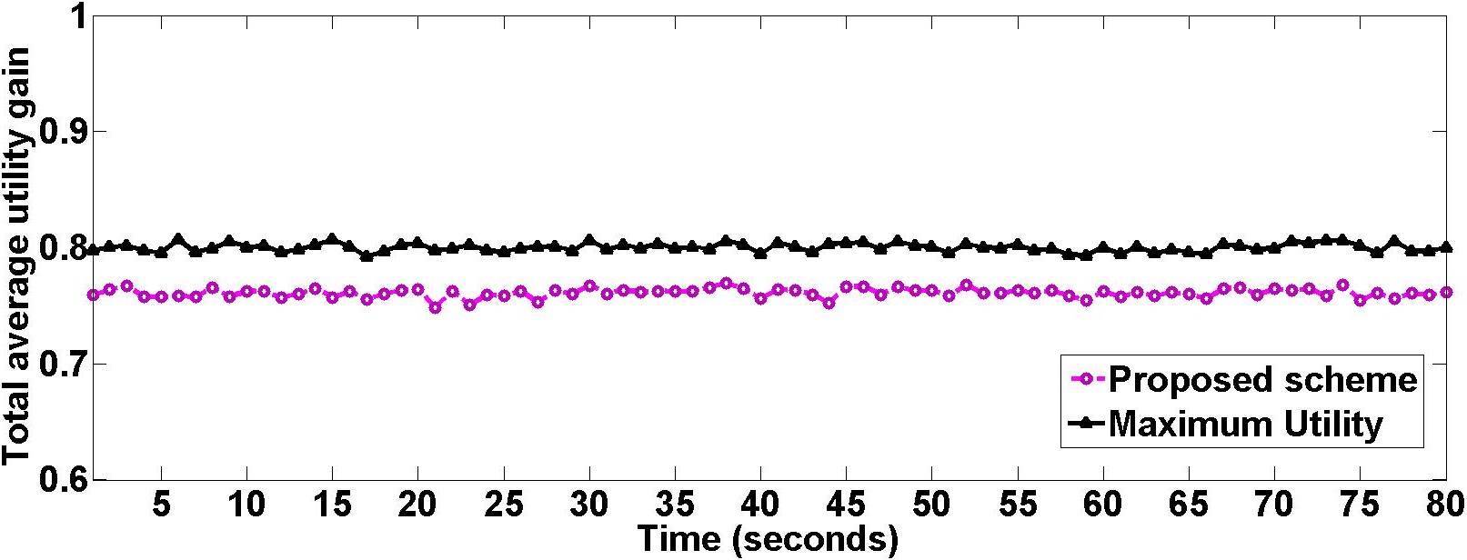
Fig. 2: Utility average of two compared schemes: Proposed and Maximum Utility

TABLE I: Utility Functions of Different Applications

Application	Utility Function	Calibration Parameters
VoIP	$U_{1}^{\Xi}=(1-FER_{eff,r}^{\Xi})\cdot\underset{i=0}{\overset{L_{T}}{\sum}}\alpha_{i}\cdot X(rate(m_{r}^{\theta}),l_{i})$	$X(x,l_{i})=\begin{cases}1&x\in l_{i}\\ 0&x\notin l_{i}\end{cases}$, where $l_{i}:\textrm{ required rate of the quality/utility level}$
		$L_{T}:\textrm{total number of levels}$, $\alpha_{i}:\textrm{scaling parameter of }l_{i}$
Video Streaming	$U_{2}^{\Xi}=(1-FER_{eff,r}^{\Xi})\cdot\frac{1}{1+(\frac{1}{\epsilon}-1)\cdot e^{-\beta\cdot rate(m_{r}^{\theta})}}$	$\beta=\frac{2\cdot\ln(\frac{1}{\epsilon}-1)}{RATE_{max}}$, where $RATE_{max}:\textrm{maximal rate requirement}$
		$\epsilon:\textrm{minimum of utility gain achievable by }RATE_{min}$, $RATE_{min}=\textrm{minimal rate requirement}$
File Transfer	$U_{3}^{\Xi}=(1-FER_{eff,r}^{\Xi})\cdot\frac{\log(rate(m_{r}^{\theta})+1)}{\log(RATE_{max}+1)}$	$RATE_{max}:\textrm{maximal rate requirement}$
Online Gaming	$U_{4}^{\Xi}=(1-FER_{eff,r}^{\Xi})\cdot\frac{1}{1+(\frac{1}{\epsilon}-1)\cdot e^{-\gamma\cdot rate(m_{r}^{\theta})}}$	$\gamma=\frac{1}{\underset{i=1}{\overset{N}{\sum}}\frac{t_{i}}{\gamma_{i}}}$, $\gamma_{i}=\frac{2\cdot\ln(\frac{1}{\epsilon}-1)}{RATE_{max,i}}$, where $RATE_{max,i}:\textrm{intrinsic rate of }t_{i}$
		$t_{i}:\textrm{traffic proportion of applications,}$ ($1\leq i\leq N$—$N:\textrm{number of applications}$)
		$\underset{i=1}{\overset{N}{\sum}}t_{i}=1$ and $\textrm{maximal rate requirement: }RATE_{max}=\underset{i=1}{\overset{N}{\sum}}t_{i}\cdot RATE_{max,i}$

In this section, we numerically evaluate the performance of the proposed optimal algorithm for the utility max-min fair link adaptation in MATLAB. The downlink channel setup is modeled based on the TGn channel models. We use profile B (residential) of those models in our simulations. In order to ensure that the model is appropriate for IEEE 802.11ac scenarios, we modified some of its parameters, including the Doppler component, the angle of arrival (AoA), and the angle of departure (AoD) according to the IEEE 802.11ac task group recommendations. The system has been configured to operate at the 5.25-GHz carrier frequency with a bandwidth of $W=20$ MHz subdivided into 64 subcarriers, 52 of which are used to carry data. There are nine different MCSs, which results in transmission rates (i.e., $rate(m_{r}^{\theta})$) ranging from 6.5 Mbps (BPSK, 1/2) to 78 Mbps (256-QAM, 5/6). The transmitter is equipped with four antennae, and each of the four receivers has only one antenna. We exploit four distinct utility functions, VoIP, video streaming, file transfer, and online gaming applications, using suggested functions in [2] and [9]. These utility functions are described in Table I. The calibration parameters for video streaming, file transfer and online gaming are set according to [9]. The VoIP utility function is calibrated by the following parameters (refer to [10] for details): $L_{T}=3$, $\alpha_{i}\in\{\alpha_{1}=0.92,\alpha_{2}=0.95,\alpha_{3}=1\}$, $l_{i}\in\{l_{1}=\{[21,32)\},l_{2}=\{[32,88)\},l_{3}=\{[88,\infty)\}\}$ (all in Kbps) and $U_{min,1}=0.7$ (for other receivers, $U_{min,2}=0.5$, $U_{min,3}=0.4$ and $U_{min,4}=0.4$) . We have concentrated on the long-time simulation scale of 20000 DL-MU transmissions, and for the presented results in this section, the width of the 95% confidence interval of the true mean is less than 5% of each plotted value.

The proposed scheme is compared with the equal power allocation (EPA) and maximum utility schemes. The EPA scheme allocates the same (max-min fair) power level to all receivers, while the maximum utility scheme selects the link adaptation policies in the manner of maximizing the total utility gain (performance gain). First, we validate the proposed scheme in terms of the Jain’s fairness index for the objective function $O_{r}^{\Xi}$’s gap between the minimum receiver utility $U_{min,r}$ and the increased max-min fair utility determined by applying policy $\rho_{r}^{sel}$ in order to obtain a quantified measure. Fig. 1 illustrates the measured results for two compared schemes. The horizontal axis is time steps (A-MPDU transmissions) and the vertical axis shows the corresponding fairness index. The index ranges from $\tfrac{1}{R}$ (worst case) to $1$ (best case) and is maximized when all receivers gain a max-min fair proportion of the utilities. We deduce that the proposed scheme guarantees a similar utility gap among the receivers while EPA performs worse with regard to fairness. Second, we indicate the efficiency of the proposed scheme by presenting the average utility gain of the proposed and maximum utility schemes. Fig. 2 demonstrates the averaged utility gains for each compared scheme (the horizontal axis is same as in Fig. 1 and the vertical axis is for utility score). Moreover, Table II represents the utility of each receiver in average (to interpret the results, note that: $U_{min,1}=0.7$, $U_{min,2}=0.5$, $U_{min,3}=0.4$ and $U_{min,4}=0.4$). We observe that the maximum utility scheme selects the policies to maximize the total utility, resulting in the best utility gain. In contrast, the proposed scheme (max-min fair) achieves the lower yet relatively close (see Fig. 2 and Table II) utility gain by paying the price of providing the max-min fairness and utility gain efficiency combined. We conclude that the proposed scheme achieves 95% of the best possible total utility gain. As analyzed before, the simulation results numerically confirm and validate the max-min fair and efficient utility gain of the receivers in the proposed scheme.

V Conclusions

In this letter, we proposed a novel model for utility max-min fair link adaptation in the IEEE 802.11ac DL-MU. We achieve the max-min fairness among the receivers using the simple, accurate, and practical link adaptation model and corresponding solution algorithms, which have been analyzed in this letter. Via simulation experiments, the solution to the proposed model scheme is investigated and validated by quantitative comparisons.

TABLE II: Receiver Utilities in Average for Two Compared Schemes.

Scenario\Average Utility	$U_{1}$	$U_{2}$	$U_{3}$	$U_{4}$
Proposed Scheme	0.9727	0.7706	0.6636	0.6371
Maximum Utility Scheme	0.8772	0.7774	0.6636	0.8820

References

- [1] Z. Cao and E. W. Zegura, “Utility max-min: An application-oriented bandwidth allocation scheme,” in Eighteenth Annual Joint Conference of the IEEE Computer and Communications Societies, INFOCOM’99, vol. 2. IEEE, 1999, pp. 793–801.
- [2] W.-H. Wang, M. Palaniswami, and S. Low, “Application-oriented flow control: Fundamentals, algorithms and fairness,” IEEE/ACM Transactions on Networking, vol. 14, no. 6, pp. 1282–1291, 2006.
- [3] M. Chiang, “Nonconvex optimization for communication networks,” in Advances in Applied Mathematics and Global Optimization, ser. Advances in Mechanics and Mathematics, D. Y. Gao and H. D. Sherali, Eds. Springer, 2009, vol. 17, pp. 137–196.
- [4] D. Halperin, W. Hu, A. Sheth, and D. Wetherall, “Predictable 802.11 packet delivery from wireless channel measurements,” in ACM SIGCOMM Computer Communication Review, vol. 40, no. 4, 2010, pp. 159–170.
- [5] “IEEE 802.11ac - amendment 4: Enhancements for very high throughput for operation in bands below 6ghz,” IEEE P802.11ac/D7.0, 2013.
- [6] A. Goldsmith and A. Nin, Wireless Communications. Cambridge University Press, 2005.
- [7] D. P. Bertsekas, R. G. Gallager, and P. Humblet, Data networks. Prentice-Hall International, 1992.
- [8] G. R. Cantieni, Q. Ni, C. Barakat, and T. Turletti, “Performance analysis under finite load and improvements for multirate 802.11,” Computer Communications, vol. 28, no. 10, pp. 1095–1109, 2005.
- [9] C. Liu, L. Shi, and B. Liu, “Utility-based bandwidth allocation for triple-play services,” in Conference on Fourth European Universal Multiservice Networks, ECUMN’07. IEEE, 2007, pp. 327–336.
- [10] A. Headquarters, “Cisco unified contact center enterprise solution reference network design (SRND).” [Online]. Available: www.cisco.com/go/srnd