Giant slip at liquid-liquid interfaces using hydrophobic ball bearings

Abstract

Liquid-gas-liquid interfaces stabilized by hydrophobic beads behave as ball bearings under shear and exhibit giant slip. Using a scaling analysis and Molecular Dynamics simulations we predict that, when the contact angle $\theta$ between the beads and the liquid is large, the slip length diverges as $R\rho^{-1}(\pi-\theta)^{-3}$ where $R$ is the bead radius, and $\rho$ is the bead density.

Starting with the seminal work of Navier in 1823 Navier (1823), the study of interfacial slip at liquid-solid interfaces has a long history. Slip is usually not observed at macroscopic scales, but the recent downsizing of hydrodynamic flows in micro and nanofluidic devices Stone et al. (2004); Bocquet and Charlaix (2010) has paved the way for measurements at small length scales. These measurements revealed that slip occurs at the nanometer scale on flat substrates Cottin-Bizonne et al. (2005); Joly et al. (2006); Bocquet and Barrat (2007); Lasne et al. (2008); Vinogradova et al. (2001). However, nature has produced surfaces such as plant leaves, with complex topographic structures (bumps, hairs, etc.) on the top of which water drops can be deposited without collapse in the so-called Cassie-Baxter (or fakir) state Cassie and Baxter (1944); Callies and Quere (2005); Shirtcliffe et al. (2010). Man-made devices based on this principle led to an increase of slip by orders of magnitude, using e.g. substrates with nanopillar arrays Choi and Kim (2006); Joseph et al. (2006); Ybert et al. (2007); Feuillebois et al. (2009); Reyssat et al. (2010); Mognetti et al. (2010). One may therefore wonder whether a similar strategy could be used to increase slip in liquid-liquid interfaces. Indeed, a few studies considering the possibility of slip at the bare interface between two simple liquids have shown that slip, if present, was negligible above the molecular scale Galliero (2010a); Hu et al. (2010). Surprisingly, virtually no work has been devoted to optimizing slip at liquid/liquid interfaces. A large liquid-liquid slip would open new possibilities in micro and nanofluidics, permitting different liquids in contact to flow independently with reduced interfacial friction. In the following, we show that it is possible to achieve giant slip between two liquids using a bed of hydrophobic beads, as depicted in Fig. 1(a).

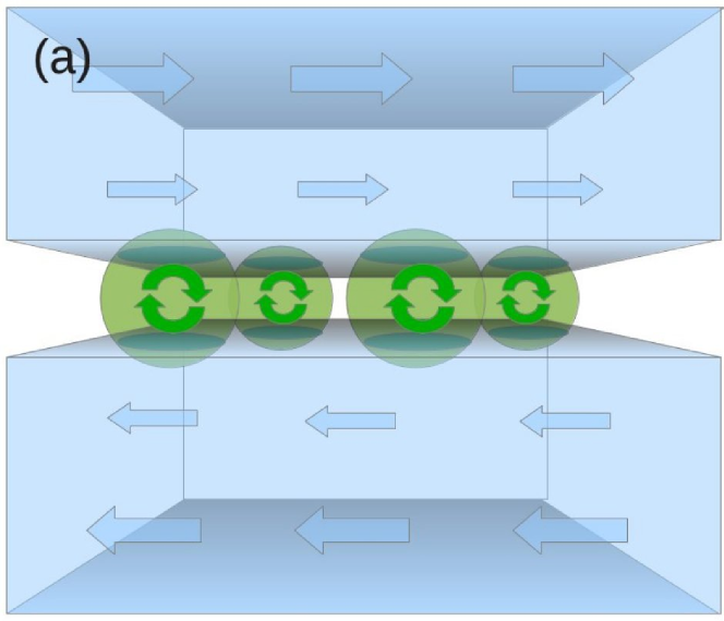
Figure 1: (color online) Schematics. (a) Using hydrophobic beads as a ball bearing to enhance liquid/liquid slip. (b) Unit cell of the periodic system analyzed in the text. (c) Expected macroscopic flow in the interface region.

Following the principle of usual ball bearings, we suggest to use an interface where hydrophobic beads maintain a gas layer between two bulk liquids. The stability of this interface is ensured by wetting forces, instead of being controlled by the contact between the beads and the solid substrate in usual ball bearings. Such a metastable configuration reminds of pillar-based superhydrophobic surfaces, used to amplify liquid-solid slippage Choi and Kim (2006); Joseph et al. (2006); Ybert et al. (2007); Feuillebois et al. (2009); Reyssat et al. (2010); Mognetti et al. (2010). In both cases the liquid rests mainly on a gas layer, leading to a low level of friction. However there are two important differences between these systems: to the advantage of hydrophobic ball bearings, beads are able to roll, thereby reducing friction at the liquid/bead interface. However beads will always penetrate inside the liquid, thereby inducing viscous dissipation, and consequently decreasing slippage. As seen in Fig. 1(a,b), the penetration depth is directly controlled by the wetting angle $\theta$ of the liquid at the bead surface. As a consequence, $\theta$ is expected to have a strong influence on the efficiency of liquid/liquid bearings. In the following, we start by quantifying analytically the influence of the wetting angle on liquid/liquid slip in this system. We then confirm the obtained scaling law by means of Molecular Dynamics (MD) simulations. Finally, we discuss the expected amplitude of slip in experimental systems.

In order to discuss the behavior of liquid-liquid bearings under shear, we shall consider a simplified geometry with a periodic array of beads. The unit cell contains a single bead, as sketched in Fig. 1(b). Shear is forced by a velocity difference $2V$ between two parallel walls separated by a distance $2L_{y}$. The $x$ and $y$ axes are indicated in the schematic, and the $z$ axis is orthogonal to the plane of the schematic. The system is assumed to be periodic along the $x$ and $z$ axes. At liquid-solid interfaces, the Navier partial slip boundary condition (BC) Navier (1823); Bocquet and Barrat (2007), $\Delta v=b\dot{\gamma}$, relates the velocity jump at the interface $\Delta v$ to the far-field shear rate $\dot{\gamma}$ inside the liquid, where $b$ is the slip length. The slip length between two liquids with the same viscosity may be defined using the same equation without ambiguity (see Supplementary material). Therefore, one can use the velocity $v^{i}$ extrapolated at the median plane passing though the center of the bead as in Fig. 1(c), leading to

$$b={2v^{i}\over\dot{\gamma}},$$ (1)

where $\dot{\gamma}=(V-v^{i})/L_{y}$ is the macroscopic shear rate in the liquid.

Focusing on small scales hydrodynamics, we investigate the limit of small Reynolds numbers and negligible gravity effects. We consider a steady state. In the referential of the bead center of mass, the solid-liquid and liquid-gas interfaces have null normal velocity (however, they can exhibit a non-vanishing tangential velocity). In such a fixed geometry, a minimum dissipation principle is available for Stokes flow (i.e. the limit of vanishing Reynolds numbers) with no-slip boundary condition as discussed historically by Helmholtz Helmholtz (1868), Rayleigh Rayleigh (1913), and Korteweg Korteweg (1868). This principle is easily extended to a variable slip length along the boundary Pierre-Louis , and therefore applies to our system, where the interface is a sum of portions of liquid-gas interface with infinite slip and liquid-solid interface with zero or partial slip. Since the walls are only an artificial setup to enforce shear, we consider a no-slip BC at the wall-liquid interface in the following. However, at the physically relevant liquid-bead interface, we shall discuss both cases of perfect slip and vanishingly small slip.

Let us start with the case of a perfect slip. The steady state corresponds to the minimization of the total viscous dissipation:

$$Q=\frac{\eta}{2}\int\mathrm{d}^{3}\mathbf{r}\left[\partial_{\mu}v_{\nu}+\partial_{\nu}v_{\mu}\right]^{2},$$ (2)

where $\mu$, $\nu$ represent $x$, $y$, or $z$, and the Einstein summation convention is assumed. Our strategy is to evaluate $Q$ as a function of the interface velocity $v^{i}$, and to select the velocity $v^{i}_{*}$ for which $Q$ is minimized. We therefore need to analyze of the flow field $\mathbf{v}=(v_{x},v_{y},v_{z})$ present in the system. The first contribution to $\mathbf{v}$ is due to the direct shear flow ${\bf v}_{D}$ imposed by the boundary conditions. In the upper part of the system, with $y>0$, we have

$${\bf v}_{D}=\left(v^{i}+y\dot{\gamma}\right)\hat{\bf x}.$$ (3)

The second contribution is the backflow ${\bf v}_{B}$ caused by the response of the system to the direct flow. We assume that the liquid-gas interface remains flat, so that the backflow is mainly caused by the presence of the bead. Its main component is along $y$:

$${\bf v}_{B}=\partial_{x}y_{s}v_{Dx}\hat{\bf y},$$ (4)

where $y_{s}(x,z)$ is the position of the liquid boundary (liquid-solid plus liquid-gas interfaces). Since $\theta\rightarrow\pi$, we have $\partial_{xx}y_{s}\approx-1/R$ and $y_{s}\approx R$ above the bead, leading to

$$\partial_{x}v_{By}\approx-{1\over R}\left(v^{i}+R\dot{\gamma}\right).$$ (5)

Using Eq. (2), the total dissipation now reads:

$$Q={\eta\over 2}\int d^{3}\mathbf{r}\left[\dot{\gamma}-{1\over R}\left(v^{i}+R\dot{\gamma}\right)\right]^{2}.$$ (6)

The backflow penetrates the liquid in a domain of volume $\ell^{3}$, where $\ell\approx 2R(\pi-\theta)$ is the lateral extent of the solid-liquid contact region. Hence, the backflow terms in the integrand of Eq. (6) should be integrated in this volume only. Using the separation of length scales $\ell\ll R\ll L_{y}$, we then find

$$Q=\eta{L_{x}L_{z}\over L_{y}}(V-v^{i})^{2}+8\eta\alpha R(\pi-\theta)^{3}(v^{i})^{2},$$ (7)

where $\alpha$ is a dimensionless prefactor accounting for the system geometry. We may now find the slip velocity $v^{i}_{*}$ which minimizes the dissipation from the equation $\partial_{v^{i}}Q_{2D}|_{v^{i}=v^{i}_{*}}=0$. Finally, using $v^{i}_{*}$ in Eq. (1), we obtain

$$b={1\over 4\rho R\alpha(\pi-\theta)^{3}},$$ (8)

where $\rho=1/(L_{x}L_{z})$ is the bead density at the interface.

The no-slip limit is more subtle, due to the expected divergence of viscous dissipation at the triple line de Gennes (1985); Huh and Scriven (1971), as the intrinsic liquid/bead slip length $b_{0}$ vanishes. This contribution enters into play as a divergence of $\partial_{xx}y_{s}$ at the triple line, replacing $1/R$ by $(\pi-\theta)/b_{0}$ in Eq. (5). Assuming that the backflow extends to a distance $b_{0}$ along the triple-line perimeter $\pi\ell$ then suggests a dissipation $\sim\eta v^{i2}\pi\ell b_{0}^{2}[(\pi-\theta)/b_{0}]^{2}\sim\eta v^{i2}R(\pi-\theta)^{3}$ as in Eq.(7). A more precise analysis based on the expansion for $\theta\rightarrow\pi$ of the exact two-dimensional solution of Stokes flow in a wedge Huh and Scriven (1971) confirms this scaling, but also indicates the presence of a logarithmic correction. Indeed, as $\theta\rightarrow\pi$ the dissipation per unit length of triple line reads $\sim\eta v^{i2}(\pi-\theta)^{2}\ln(\ell_{0}/b_{0})$, where $\ell_{0}$ is a macroscopic cutoff. Assuming $\ell_{0}\sim\ell$, we obtain a dissipation $\sim\eta v^{i2}R(\pi-\theta)^{3}\ln[(\pi-\theta)R/b_{0}]$, from which we compute $b\sim 1/\{R(\pi-\theta)^{3}\ln[(\pi-\theta)R/b_{0}]\}$. We therefore expect the scaling behavior in Eq. (8) to be weakly affected (i.e. within logarithmic corrections) by the boundary condition between the liquid and the bead.

Note that our analysis relies on the assumption that $\theta$ does not depend on the triple-line velocity. This should be achieved for low capillary numbersde Gennes (1985). In this limit, $\theta$ does not depend on $\eta$, and thus Eq.(8) indicates that $b$ should be independent of $\eta$.

In order to test the predictions of Eq. (8), we performed molecular dynamics (MD) simulations, using the LAMMPS package Plimpton (1995). We consider once again a periodic array of beads, the unit cell of which is presented in Fig. 2.

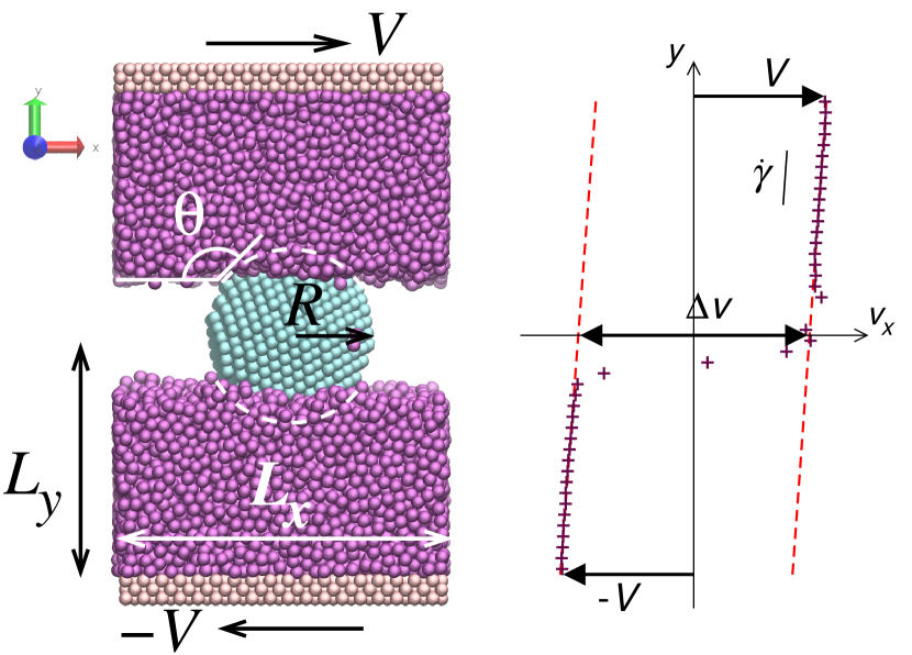
Figure 2: (color online) Snapshot of a typical molecular dynamics system (created using VMD Humphrey et al. (1996)), with the associated steady-state velocity profile on the right.

All atoms interacted via a Lennard-Jones (LJ) pair potential: $V_{ij}=4\varepsilon_{ij}[(\sigma/r)^{12}-(\sigma/r)^{6}]$, where $i$ and $j$ are the types of interacting atoms, and $r$ and $\varepsilon_{ij}$ are respectively their distance and interaction energy. The zero-potential distance $\sigma$ is the same for all atom types. In addition, we chose the fluid-fluid interaction energy as the reference energy $\varepsilon_{ff}=\varepsilon$. In the following, we will use LJ units of energy $\varepsilon$, distance $\sigma$, and time $\tau=\sigma\sqrt{m/\varepsilon}$, where $m$ is the atomic mass. In order to increase the liquid/vapor surface tension and to decrease the vapor density as compared to a simple LJ liquid, we used a liquid of LJ dimers Galliero (2010b), i.e. pairs of LJ atoms bonded by a harmonic potential. We used a dissipative particle dynamics (DPD) thermostat to maintain the liquid atoms at a temperature $k_{\mathrm{B}}T=0.73\varepsilon$ while preserving hydrodynamics Groot and Warren (1997). The bead was modeled as a rigid spherical shell of radius $R=7.07\sigma$ (with a thickness larger than the LJ cutoff $2.5\sigma$), cut inside a fcc crystal with density $1/\sigma^{3}$. The confining walls were made of three (010) layers of frozen atoms on a fcc lattice, with the same density $1/\sigma^{3}$. The contact angle is controlled by the fluid-solid interaction energy in the LJ potential. We used $\varepsilon_{fw}=0.7\varepsilon$ between fluid and wall atoms, so as to ensure a small contact angle, and consequently a no-slip BC Huang et al. (2008). In contrast, the fluid-bead interaction energy $\varepsilon_{fb}$ was tuned in order to change the contact angle $\theta$. The latter was then computed from in situ measurements of the vapor gap width. Finally, the distance between the top of the bead and the walls was $\approx 2R$ in all simulations. This was large enough to remove in practice the influence of the confining walls, and to allow for a linear average velocity profile in the liquid which enables the measurement of the shear rate $\dot{\gamma}$. After a period of equilibration, the system was sheared by imposing opposite wall velocities $\pm V$ along $x$. All along the simulation, both walls were used as pistons to impose a vanishing pressure inside the system.

To measure $b$, we first used the kinematic definition, Eq. (1). In order to extract $\Delta v$ and $\dot{\gamma}$, we fitted the numerical velocity profiles in the linear regions between the bead and the walls, as shown in Fig. 2. However, for large contact angles, the shear rate $\dot{\gamma}$ becomes increasingly small, and its measurement in the fluid is inaccurate. We therefore resort to a different definition of the slip length based on a dynamic interpretation Falk et al. (2010). On the one hand, the bulk viscous shear stress is $\eta\dot{\gamma}$, where $\eta$ is the liquid viscosity. On the other hand, the interface shear stress equals the interfacial friction force $f$ per unit area, which is proportional to the velocity jump: $f=\lambda\Delta v$. This latter relation defines the interfacial friction coefficient $\lambda$. Equating the bulk and interface shear stresses, one recovers the partial slip BC with $b=\eta/\lambda$. Therefore, the slip length can also be computed as the ratio between the bulk liquid viscosity and the interfacial friction coefficient. The liquid viscosity $\eta\approx 5.52$ LJ units, was determined under the same thermodynamic conditions in independent shear flow simulations. The friction coefficient $\lambda$ was computed as the ratio of the measured shear force per unit area $f$ and the measured velocity jump $\Delta v$. For the analysis of the non-trivial $\theta$-dependence of $b$, we used a fixed box size $L_{x}=L_{z}=4R$, corresponding to $\rho=1/(16R^{2})$. In Fig. 3, the resulting slip length is plotted as a function of $\theta$.

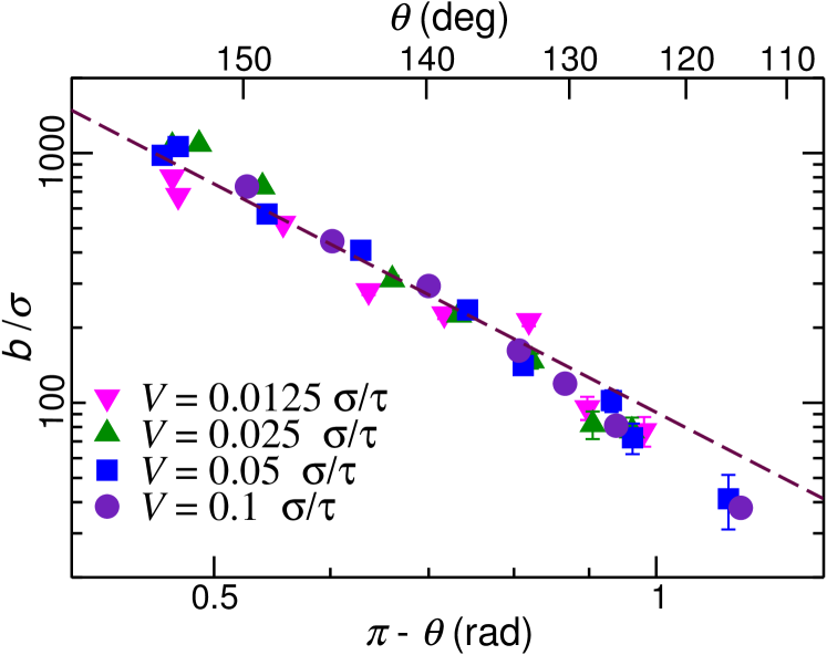
Figure 3: (color online) Slip length $b$ as a function of the measured wetting angle $\theta$, using the dynamic definition of the slip length. Data set keys indicate the shear velocity $V$, in LJ units ($\sigma/\tau$). All data sets collapse on a master curve $b\propto(\pi-\theta)^{-3}$ (dashed line).

Using the dynamic method, all data points collapse on a single master curve $b\propto(\pi-\theta)^{-3}$, as predicted by Eq. (8). The fit to Eq. (8) provides a value for the dimensionless prefactor $\alpha=0.31{\pm 0.02}$. The results of the kinematic method are similar to those of the dynamic method. However, as anticipated above, the kinematic method is less precise at small shear rates, leading to larger scatter of the data. The comparison between the results of the two methods is provided in Supplementary Material. We have also checked that $b\sim 1/\rho$, as predicted by Eq. (8). Deviations from this latter scaling are observed when hydrodynamic interactions come into play at high bead-density and when $\pi-\theta$ is not small. Details are discussed in Supplementary Material.

A recurrent issue in MD simulations is the need to use a very large forcing in order to extract the system response out of thermal noise. Such large driving forces could lead to a nonlinear response, questioning the description of the interface behavior by means of a slip length. Our shear rates were $\sim 10^{7}$ to $10^{9}$ Hz, which is very large as compared to experimentally relevant shear rates, typically smaller than $10^{5}$ Hz. As shown in Fig. 3, we varied $V$ over almost one order of magnitude and checked that the measured slip lengths remained unaffected. We may therefore conclude that the system response is linear, and can be safely extrapolated to the much lower experimental shear rates. In addition, it is clear from the adequacy between Eq.(8) and MD simulations that thermal fluctuations play a negligible role in the emergent macroscopic behavior, at least in the explored parameter range.

Finally, note that we do not control the slip at the liquid-bead interface in our MD simulations. It is known that both the contact angle and the curvature of the solid surface may have a strong impact on the liquid-bead slipHuang et al. (2008); Einzel et al. (1990). However, as discussed above, the variation of the liquid-bead slip length $b_{0}$ is not crucial for our main result Eq. (8), and should lead to minor logarithmic corrections, the discussion of which are beyond the scope of the present Letter.

Interfaces similar to that of Fig.1(a) have actually already been observed experimentally using liquid marbles floating on liquid substratesQuéré (2002); Bormashenko et al. (2012). However, to our knowledge no analysis of slip has been performed for these interfaces. An important way to reduce slip in these systems is to decrease the bead density, which directly enters into the expression of $b$ in Eq.(8). In addition, lowering the density may help to prevent contact and friction between the beads, which is expected have negative consequences on slip. One possible way to control the density is to use electrostatic repulsion between the beads along the same lines as the in formation of colloidal Wigner crystals at water-oil interfaces Irvine et al. (2010). Let us assume that one could build such a system, with typical densities $\rho$ varying from $0.01R^{-2}$ to $0.1R^{-2}$. Assuming $0.03R^{-2}$ (corresponding to a distance of about two diameters between the beads), Eq.(8) predicts $b\approx 20R$ with $\theta=120\,^{\circ}$, and $b\approx 200R$ with $\theta=150\,^{\circ}$ (using e.g. superhydrophobic beads). With a bead radius $R=10\,\mu$m, $b$ would therefore be on the scale of millimeters for large contact angles ($b\approx 0.2$ and $2$ mm for $\theta=120$ and $150\,^{\circ}$ respectively).

In our opinion, a strong limitation of this giant slip is the stability of the interface under pressure variations. Two processes are involved. First, the Laplace-pressure-induced curvature of the liquid-gas interface imposes an additional backflow, increasing dissipation. This effect is similar to the effect of pressure in pillar-based superhydrophobic surfaces Steinberger et al. (2007); Biben and Joly (2008). Defining the curvature $\kappa$ of the liquid-gas interface, and assuming that the related backflow extends in the liquid up to a distance similar to the inter-bead distance, we obtain an additional dissipation $\sim\eta\rho^{-3/2}\kappa^{2}(v^{i})^{2}$ in Eq. (7). Recalling the Laplace law $\kappa=\Delta P/2\gamma$, where $\Delta P$ is the pressure variation and $\gamma$ is the surface tension, we obtain a correction of the slip length $b^{-1}=b^{-1}|_{\Delta P=0}+\alpha^{\prime}\rho^{-1/2}(\Delta P)^{2}/4\gamma^{2}$ with $\alpha^{\prime}$ a constant of order one, showing that $b$ decreases when increasing $|\Delta P|$. The correction is negligible when $|\Delta P|<2\gamma\rho^{1/4}b^{-1/2}$, where the zero-pressure slip length $b$ is given by Eq. (8). This condition becomes stringent when $b$ is large, and for $\theta=150\,^{\circ}$ with $R=10\,\mu$m, one obtains $|\Delta P|<8$ mbar. The second limitation related to the pressure is the possibility of contact between the two opposite liquid-gas interfaces, leading to the collapse of the system. Balancing the typical interface displacement $\kappa\rho^{-1}$ with the typical average separation $\sim R$, the collapse will be avoided when $\Delta P<2\gamma R\rho$. Using $R=10\,\mu$m and $\rho=0.03R^{-2}$, one finds again $P<4$ mbar. The stability can be enhanced, at the cost of a smaller slip length, by using higher densities and smaller beads. For instance, with $R=0.1\,\mu$m and $\rho=0.1R^{-2}$, one finds $P<1$ bar, but $b\approx 6\,\mu$m for $\theta=150\,^{\circ}$.

In conclusion, giant slip can be obtained between two liquids using hydrophobic ball bearings. We hope that this work will motivate experimental investigations of the dynamic properties of such interfaces. Liquid-liquid bearings open new pathways for micro- and nano-fluidics research. One major direction could be to build fluidic devices without walls, where different liquids could flow with regard to each other while maintaining an extremely low level of friction, and preventing mixing by diffusion between the different channels.