Efficient Synthesis of Network Updates

Abstract

Software-defined networking (SDN) is revolutionizing the networking industry, but current SDN programming platforms do not provide automated mechanisms for updating global configurations on the fly. Implementing updates by hand is challenging for SDN programmers because networks are distributed systems with hundreds or thousands of interacting nodes. Even if initial and final configurations are correct, naïvely updating individual nodes can lead to incorrect transient behaviors, including loops, black holes, and access control violations. This paper presents an approach for automatically synthesizing updates that are guaranteed to preserve specified properties. We formalize network updates as a distributed programming problem and develop a synthesis algorithm based on counterexample-guided search and incremental model checking. We describe a prototype implementation, and present results from experiments on real-world topologies and properties demonstrating that our tool scales to updates involving over one-thousand nodes.

1 Introduction

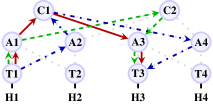
Figure 1: Example topology.

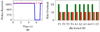
Figure 2: Example naïve (blue/solid-line), two-phase (green/solid-bar), and ordering (red/dashed) updates: (a) probes received; (b) per-switch rule overhead.

Software-defined networking (SDN) is a new paradigm in which a logically-centralized controller manages a collection of programmable switches. The controller responds to events such as topology changes, shifts in traffic load, or new connections from hosts, by pushing forwarding rules to the switches, which process packets efficiently using specialized hardware. Because the controller has global visibility and full control over the entire network, SDN makes it possible to implement a wide variety of network applications ranging from basic routing to traffic engineering, datacenter virtualization, fine-grained access control, etc. Casado et al. [2014]. SDN has been used in production enterprise, datacenter, and wide-area networks, and new deployments are rapidly emerging.

Much of SDN’s power stems from the controller’s ability to change the global state of the network. Controllers can set up end-to-end forwarding paths, provision bandwidth to optimize utilization, or distribute access control rules to defend against attacks. However, implementing these global changes in a running network is not easy. Networks are complex systems with many distributed switches, but the controller can only modify the configuration of one switch at a time. Hence, to implement a global change, an SDN programmer must explicitly transition the network through a sequence of intermediate configurations to reach the intended final configuration. The code needed to implement this transition is tedious to write and prone to error—in general, the intermediate configurations may exhibit new behaviors that would not arise in the initial and final configurations.

Problems related to network updates are not unique to SDN. Traditional distributed routing protocols also suffer from anomalies during periods of reconvergence, including transient forwarding loops, blackholes, and access control violations. For users, these anomalies manifest themselves as service outages, degraded performance, and broken connections. The research community has developed techniques for preserving certain invariants during updates Francois and Bonaventure [2007]; Raza et al. [2011]; Vanbever et al. [2011], but none of them fully solves the problem, as they are limited to specific protocols and properties. For example, consensus routing uses distributed snapshots to ensure connectivity, but only applies to the Border Gateway Protocol (BGP) John et al. [2008].

It might seem that SDN would exacerbate update-related problems by making networks even more dynamic—in particular, most current platforms lack mechanisms for implementing updates in a graceful way. However, SDN offers opportunities to develop high-level abstractions for implementing updates automatically while preserving key invariants. The authors of B4—the controller managing Google’s world-wide inter-datacenter network—describe a vision where: “multiple, sequenced manual operations [are] not involved [in] virtually any management operation” Jain et al. [2013].

Previous work proposed the notion of a consistent update Reitblatt et al. [2012], which ensures that every packet is processed either using the initial configuration or the final configuration but not a mixture of the two. Consistency is a powerful guarantee preserving all safety properties, but it is expensive. The only general consistent update mechanism is two-phase update, which tags packets with versions and maintains rules for the initial/final configurations simultaneously. This leads to problems on switches with limited memory and can also make update time slower due to the high degree of rule churn.

We propose an alternative. Instead of forcing SDN operators to implement updates by hand (as is typically done today), or using powerful but expensive mechanisms like two-phase update, we develop an approach for synthesizing correct update programs efficiently and automatically from formal specifications. Given initial and final configurations and a Linear Temporal Logic (LTL) property capturing desired invariants during the update, we either generate an SDN program that implements the initial-to-final transition while ensuring that the property is never violated, or fail if no such program exists. Importantly, because the synthesized program is only required to preserve the specified properties, it can leverage strategies that would be ruled out in other approaches. For example, if the programmer specifies a trivial property, the system can update switches in any order. However, if she specifies a more complex property (e.g. firewall traversal) then the space of possible updates is more constrained. In practice, our synthesized programs require less memory and communication than competing approaches.

Programming updates correctly is challenging due to the concurrency inherent in networks—switches may interleave packet and control message processing arbitrarily. Hence, programmers must carefully consider all possible event orderings, inserting synchronization primitives as needed. Our algorithm works by searching through the space of possible sequences of individual switch updates, learning from counterexamples and employing an incremental model checker to re-use previously computed results. Our model checker is incremental in the sense that it exploits the loop-freedom of correct network configurations to enable efficient re-checking of properties when the model changes. Because the synthesis algorithm poses a series of closely-related model checking questions, the incrementality yields enormous performance gains on real-world update scenarios.

We have implemented the algorithm and heuristics to further speed up synthesis and eliminate spurious synchronization. We have interfaced the tool with Frenetic Foster et al. [2011], synthesized updates for OpenFlow switches, and used our system to process actual traffic generated by end-hosts. We ran experiments on a suite of real-world topologies, configurations, and properties—our results demonstrate the effectiveness of synthesis, which scales to over one-thousand switches, and incremental model checking, which outperforms a popular symbolic model checker used in batch mode, and a state-of-the-art network model checker used in incremental mode.

In summary, the main contributions of this paper are:

• We investigate using synthesis to automatically generate network updates (§2).

• We develop a simple operational model of SDN and formalize the network update problem precisely (§3).

• We design a counterexample-guided search algorithm that solves instances of the network update problem, and prove this algorithm to be correct (§4).

• We present an incremental LTL model checker for loop-free models (§5).

• We describe an OCaml implementation with backends to third-party model checkers and conduct experiments on real-world networks and properties, demonstrating strong performance improvements (§6). $\dagger$

Overall, our work takes a challenging network programming problem and automates it, yielding a powerful tool for building dynamic SDN applications that ensures correct, predictable, and efficient network behavior during updates.

2 Overview

To illustrate key challenges related to network updates, consider the network in Figure 2. It represents a simplified datacenter topology Al-Fares et al. [2008] with core switches (C1 and C2), aggregation switches (A1 to A4), top-of-rack switches (T1 to T4), and hosts (H1 to H4). Initially, we configure switches to forward traffic from H1 to H3 along the solid/red path: T1-A1-C1-A3-T3. Later, we wish to shift traffic from the red path to the dashed/green path, T1-A1-C2-A3-T3 (perhaps to take C1 down for maintenance). To implement this update, the operator must modify forwarding rules on switches A1 and C2, but note that certain update sequences break connectivity—e.g., updating A1 followed by C2 causes packets to be forwarded to C2 before it is ready to handle them. Figure 2(a) demonstrates this with a simple experiment performed using our system. Using the Mininet network simulator and OpenFlow switches, we continuously sent ICMP (ping) probes during a “naïve” update (blue/solid line) and the ordering update synthesized by our tool (red/dashed line). With the naïve update, 100% of the probes are lost during an interval, while the ordering update maintains connectivity.

Consistency.

Previous work Reitblatt et al. [2012] introduced the notion of a consistent update and also developed general mechanisms for ensuring consistency. An update is said to be consistent if every packet is processed entirely using the initial configuration or entirely using the final configuration, but never a mixture of the two. For example, updating A1 followed by C2 is not consistent because packets from H1 to H3 might be dropped instead of following the red path or the green path. One might wonder whether preserving consistency during updates is important, as long as the network eventually reaches the intended configuration, since most networks only provide best-effort packet delivery. While it is true that errors can be masked by protocols such as TCP when packets are lost, there is growing interest in strong guarantees about network behavior. For example, consider a business using a firewall to protect internal servers, and suppose that they decide to migrate their infrastructure to a virtualized environment like Amazon EC2. To ensure that this new deployment is secure, the business would want to maintain the same isolation properties enforced in their home office. However, a best-effort migration strategy that only eventually reaches the target configuration could step through arbitrary intermediate states, some of which may violate this property.

Two-Phase Updates.

Previous work introduced a general consistency-preserving technique called two-phase update Reitblatt et al. [2012]. The idea is to explicitly tag packets upon ingress and use these version tags to determine which forwarding rules to use at each hop. Unfortunately, this has a significant cost. During the transition, switches must maintain forwarding rules for both configurations, effectively doubling the memory requirements needed to complete the update. This is not always practical in networks where the switches store forwarding rules using ternary content-addressable memories (TCAM), which are expensive and power-hungry. Figure 2(b) shows the results of another simple experiment where we measured the total number of rules on each switch: with two-phase updates, several switches have twice the number of rules compared to the synthesized ordering update. Even worse, it takes a non-trivial amount of time to modify forwarding rules—sometimes on the order of 10ms per rule Jin et al. [2014]! Hence, because two-phase updates modify a large number of rules, they can increase update latency. These overheads can make two-phase updates a non-starter.

Ordering Updates.

Our approach is based on the observation that consistent (two-phase) updates are overkill in many settings. Sometimes consistency can be achieved by simply choosing a correct order of switch updates. We call this type of update an ordering update. For example, to update from the red path to the green path, we can update C2 followed by A1. Moreover, even when we cannot achieve full consistency, we can often still obtain sufficiently strong guarantees for a specific application by carefully updating the switches in a particular order. To illustrate, suppose that instead of shifting traffic to the green path, we wish to use the blue (dashed-and-dotted) path: T1-A2-C1-A4-T3. It is impossible to transition from the red path to the blue path by ordering switch updates without breaking consistency: we can update A2 and A4 first, as they are unreachable in the initial configuration, but if we update T1 followed by C1, then packets can traverse the path T1-A2-C1-A3-T3, while if we update C1 followed by T1, then packets can traverse the path T1-A1-C1-A4-T3. Neither of these alternatives is allowed in a consistent update. This failure to find a consistent update hints at a solution: if we only care about preserving connectivity between H1 and H3, then either path is actually acceptable. Thus, either updating C1 before T1, or T1 before C1 would work. Hence, if we relax strict consistency and instead provide programmers with a way to specify properties that must be preserved across an update, then ordering updates will exist in many situations. Recent work Mahajan and Wattenhofer [2013]; Jin et al. [2014] has explored ordering updates, but only for specific properties like loop-freedom, blackhole-freedom, drop-freedom, etc. Rather than handling a fixed set of “canned” properties, we use a specification language that is expressive enough to encode these properties and others, as well as conjunctions/disjunctions of properties—e.g. enforcing loop-freedom and service-chaining during an update.

In-flight Packets and Waits.

Sometimes an additional synchronization primitive is needed to generate correct ordering updates (or correct two-phase updates, for that matter). Suppose we want to again transition from the red path to blue one, but in addition to preserving connectivity, we want every packet to traverse either A2 or A3 (this scenario might arise if those switches are actually middleboxes which scrub malicious packets before forwarding). Now consider an update that modifies the configurations on A2, A4, T1, C1, in that order. Between the time that we update T1 and C1, there might be some packets that are forwarded by T1 before it is updated, and are forwarded by C1 after it is updated. These packets would not traverse A2 or A3, and so indicate a violation of the specification. To fix this, we can simply pause after updating T1 until any packets it previously forwarded have left the network. We thus need a command “wait” that pauses the controller for a sufficient period of time to ensure that in-flight packets have exited the network. Hence, the correct update sequence for this example would be as above, with a “wait” between T1 and C1. Note that two-phase updates also need to wait, once per update, since we must ensure that all in-flight packets have left the network before deleting the old version of the rules on switches. Other approaches have traded off control-plane waiting for stronger consistency, e.g. Ludwig et al. [2014] performs updates in “rounds” that are analogous to “wait” commands, and Consensus Routing John et al. [2008] relies on timers to obtain wait-like functionality. Note that the single-switch update time can be on the order of seconds Jin et al. [2014]; Lazaris et al. [2014], whereas typical datacenter transit time (the time for a packet to traverse the network) is much lower, even on the order of microseconds Alizadeh et al. [2010]. Hence, waiting for in-flight packets has a negligible overall effect. In addition, our reachability-based heuristic eliminates most waits in practice.

Summary.

This paper presents a sound and complete algorithm and implementation for synthesizing a large class of ordering updates efficiently and automatically. The updates we generate initially modify each switch at most once and “wait” between updates to switches, but a heuristic removes an overwhelming majority of unnecessary waits in practice. For example, in switching from the red path to the blue path (while preserving connectivity from H1 to H3, and making sure that each packet visits either A3 or A4), our tool produces the following sequence: update A2, then A4, then T1, then wait, then update C1. The resulting update can be executed using the Frenetic SDN platform and used with OpenFlow switches—e.g., we generated Figure 2 (a-b) using our tool.

3 Preliminaries and Network Model

  $\begin{array}[]{@{~}l@{~~}|@{~~}l@{~~}|@{~~}l@{~}}{}\lx@intercol\begin{array}[]{llcl}\textit{Switch}&\mathit{sw}&\in&\mathbb{N}\\ \textit{Port}&\mathit{pt}&\in&\mathbb{N}\\ \textit{Host}&\mathit{h}&\in&\mathbb{N}\\ \textit{Priority}&\mathit{pri}&\in&\mathbb{N}\\ \textit{Epoch}&\mathit{ep}&\in&\mathbb{N}\\ \textit{Field}&\mathit{f}&\mathord{::=}&\mathit{src}\mid\mathit{dst}\mid\mathit{typ}\mid..\\ \end{array}\hfil~{}~{}\vrule~{}~{}&\begin{array}[]{llcl}\textit{Packet}&\mathit{pkt}&\mathord{::=}&\{\mathit{f}_{1};..;\mathit{f}_{k}\}\\ \textit{Pair}&\mathit{pr}&\mathord{::=}&(\mathit{pkt},\mathit{pt})\\ \textit{Pattern}&\mathit{pat}&\mathord{::=}&\{\mathit{pt}?;\mathit{f}_{1}?;..;\mathit{f}_{k}?\}\\ \textit{Action}&\mathit{act}&\mathord{::=}&\mathit{fwd}~{}\mathit{pt}\mid\mathit{f}\mathord{:=}n\\ \textit{Rule}&\mathit{rul}&\mathord{::=}&\{\mathit{pri};\mathit{pat};\mathit{acts}\}\\ \textit{Table}&\mathit{tbl}&\mathord{::=}&\mathit{ruls}\\ \end{array}\hfil~{}~{}\vrule~{}~{}&\begin{array}[]{llcl}\textit{Location}&\mathit{loc}&\mathord{::=}&\mathit{h}\mid(\mathit{sw},\mathit{pt})\\ \textit{Command}&\mathit{cmd}&\mathord{::=}&(\mathit{sw},\mathit{tbl})\mid\mathit{incr}\mid\mathit{flush}\\ \textit{Switch}&S&\mathord{::=}&\{\mathit{sw};\mathit{tbl};\mathit{prs}\}\\ \textit{Link}&L&\mathord{::=}&\{\mathit{loc};\mathit{pkts};\mathit{loc}^{\prime}\}\\ \textit{Controller}&C&\mathord{::=}&\{\mathit{cmds};\mathit{ep}\}\\ \textit{Element}&E&\mathord{::=}&S\mid L\mid C\\ \end{array}\hfil~{}\end{array}$  Data Plane $\displaystyle\displaystyle{\hbox{\hskip 93.8932pt\vbox{\hbox{\hskip-93.89319pt\hbox{\hbox{$\displaystyle\displaystyle L.\mathit{loc}=\mathit{h}\quad\;L.\mathit{loc}^{\prime}=(\mathit{sw}^{\prime},\mathit{pt}^{\prime})\quad\;L.\mathit{pkts}=\mathit{pkts}\quad\;C.\mathit{ep}=\mathit{ep}$}}}\vbox{}}}\over\hbox{\hskip 62.90518pt\vbox{\vbox{}\hbox{\hskip-62.90518pt\hbox{\hbox{$\displaystyle\displaystyle C,\;L\xrightarrow{}C,\;\{L~{}\text{with}~{}\mathit{pkts}=\mathit{pkt}^{\mathit{ep}}\mathord{::}\mathit{pkts}\}$}}}}}}$ In      $\displaystyle\displaystyle{\hbox{\hskip 86.97842pt\vbox{\hbox{\hskip-86.97842pt\hbox{\hbox{$\displaystyle\displaystyle L.\mathit{loc}=(\mathit{sw},\mathit{pt})\quad\;L.\mathit{loc}^{\prime}=\mathit{h}\quad\;L.\mathit{pkts}=(\mathit{pkt}^{\mathit{ep}}\mathord{::}\mathit{pkts})$}}}\vbox{}}}\over\hbox{\hskip 60.39743pt\vbox{\vbox{}\hbox{\hskip-60.39743pt\hbox{\hbox{$\displaystyle\displaystyle L\xrightarrow{(\mathit{sw},\mathit{pt},\mathit{pkt})}\{L~{}\text{with}~{}\mathit{pkts}=\mathit{pkts}\}$}}}}}}$ Out      $\displaystyle\displaystyle{\hbox{\hskip 168.64978pt\vbox{\hbox{\hskip-168.64977pt\hbox{\hbox{$\displaystyle\displaystyle L.loc^{\prime}=(\mathit{sw},\mathit{pt})\quad\;L.\mathit{pkts}=(\mathit{pkt}^{\mathit{ep}}\mathord{::}\mathit{pkts})\quad\;S.\mathit{sw}=\mathit{sw}\quad\;[\![S.\mathit{tbl}]\!](\mathit{pkt},\mathit{pt})=\{(\mathit{pkt}_{1},\mathit{pt}_{1}),..,(\mathit{pkt}_{n},\mathit{pt}_{n})\}$}}}\vbox{}}}\over\hbox{\hskip 150.44061pt\vbox{\vbox{}\hbox{\hskip-150.4406pt\hbox{\hbox{$\displaystyle\displaystyle L,S\xrightarrow{(\mathit{sw},\mathit{pt},\mathit{pkt})}\{L~{}\text{with}~{}\mathit{pkts}=\mathit{pkts}\},\{S~{}\text{with}~{}\mathit{prs}=S.\mathit{prs}\uplus\{(\mathit{pkt}_{1}^{\mathit{ep}},\mathit{pt}_{1}),..,(\mathit{pkt}_{n}^{\mathit{ep}},\mathit{pt}_{n})\}\}$}}}}}}$ Process      $\displaystyle\displaystyle{\hbox{\hskip 98.01799pt\vbox{\hbox{\hskip-98.01797pt\hbox{\hbox{$\displaystyle\displaystyle S.\mathit{sw}=\mathit{sw}\quad\;S.\mathit{prs}=\{(\mathit{pkt}^{\mathit{ep}},\mathit{pt})\}\uplus\mathit{prs}\quad\;L.\mathit{loc}=(\mathit{sw},\mathit{pt})\quad\;$}}}\vbox{}}}\over\hbox{\hskip 99.5459pt\vbox{\vbox{}\hbox{\hskip-99.54588pt\hbox{\hbox{$\displaystyle\displaystyle S,\;L\xrightarrow{}\{S~{}\text{with}~{}\mathit{prs}=\mathit{prs}\},\;\{L~{}\text{with}~{}\mathit{pkts}=L.\mathit{pkts}@[\mathit{pkt}^{\mathit{ep}}]\}$}}}}}}$ Forward  Control Plane and Abstract Machine $\displaystyle\displaystyle{\hbox{\hskip 65.71735pt\vbox{\hbox{\hskip-65.71735pt\hbox{\hbox{$\displaystyle\displaystyle C.\mathit{cmds}=((\mathit{sw},\mathit{tbl})\mathord{::}\mathit{cmds})\quad\;S.\mathit{sw}=\mathit{sw}$}}}\vbox{}}}\over\hbox{\hskip 83.91803pt\vbox{\vbox{}\hbox{\hskip-83.91803pt\hbox{\hbox{$\displaystyle\displaystyle C,\;S\xrightarrow{}\{C~{}\text{with}~{}\mathit{cmds}=\mathit{cmds}\},\;\{S~{}\text{with}~{}\mathit{tbl}=\mathit{tbl}\}$}}}}}}$ Update      $\displaystyle\displaystyle{\hbox{\hskip 38.08952pt\vbox{\hbox{\hskip-38.08952pt\hbox{\hbox{$\displaystyle\displaystyle C.\mathit{cmds}=(\mathit{incr}\mathord{::}\mathit{cmds})$}}}\vbox{}}}\over\hbox{\hskip 68.03241pt\vbox{\vbox{}\hbox{\hskip-68.0324pt\hbox{\hbox{$\displaystyle\displaystyle C\xrightarrow{}\{C~{}\text{with}~{}\mathit{cmds}=\mathit{cmds};\mathit{ep}=C.\mathit{ep}+1\}$}}}}}}$ Incr      $\displaystyle\displaystyle{\hbox{\hskip 98.72244pt\vbox{\hbox{\hskip-98.72244pt\hbox{\hbox{$\displaystyle\displaystyle C.\mathit{cmds}=(\mathit{flush}\mathord{::}\mathit{cmds})\quad\;\mathit{ep}(S_{1},..,S_{k},\;L_{1},..,L_{m})=C.\mathit{ep}$}}}\vbox{}}}\over\hbox{\hskip 117.17424pt\vbox{\vbox{}\hbox{\hskip-117.17422pt\hbox{\hbox{$\displaystyle\displaystyle S_{1},..,S_{k},\;L_{1},..,L_{m},\;C\xrightarrow{}S_{1},..,S_{k},\;L_{1},..,L_{m},\;\{C~{}\text{with}~{}\mathit{cmds}=\mathit{cmds}\}$}}}}}}$ Flush      $\displaystyle\displaystyle{\hbox{\hskip 14.77893pt\vbox{\hbox{\hskip-14.77892pt\hbox{\hbox{$\displaystyle\displaystyle\mathit{Es}_{1}\xrightarrow{o}\mathit{Es}_{1}^{\prime}$}}}\vbox{}}}\over\hbox{\hskip 31.61896pt\vbox{\vbox{}\hbox{\hskip-31.61894pt\hbox{\hbox{$\displaystyle\displaystyle\mathit{Es}_{1}\uplus\mathit{Es}_{2}\xrightarrow{o}\mathit{Es}_{1}^{\prime}\uplus\mathit{Es}_{2}$}}}}}}$ Congruence  

Figure 3: Network model.

To facilitate precise reasoning about networks during updates, we develop a formal model in the style of Chemical Abstract Machine Berry and Boudol [1990]. This model captures key network features using a simple operational semantics. It is similar to the one used by Guha et al. [2013], but is streamlined to model features most relevant to updates.

3.1 Network Model

Basic structures.

Each switch $\mathit{sw}$, port $\mathit{pt}$, or host $\mathit{h}$ is identified by a natural number. A packet $\mathit{pkt}$ is a record of fields containing header values such as source and destination address, protocol type, and so on. We write $\{f_{1};\dots;f_{k}\}$ for the type of packets having fields $f_{i}$ and use “dot” notation to project fields from records. The notation $\{r~{}\text{with}~{}f=v\}$ denotes functional update of $r.f$.

Forwarding Tables.

A switch configuration is defined in terms of forwarding rules, where each rule has a pattern $\mathit{pat}$ specified as a record of optional packet header fields and a port, a list of actions $\mathit{act}$ that either forward a packet out a given port ($\mathit{fwd}~{}pt$) or modify a header field ($f\mathord{:=}n$), and a priority that disambiguates rules with overlapping patterns. We write $\{\mathit{pt}?;f_{1}?;\dots;f_{k}?\}$ for the type of patterns, where the question mark denotes an option type. A set of such rules $\mathit{ruls}$ forms a forwarding table $\mathit{tbl}$. The semantic function $[\![\mathit{tbl}]\!]$ maps packet-port pairs to multisets of such pairs, finding the highest-priority rule whose pattern matches the packet and applying the corresponding actions. If there are multiple matching rules with the same priority, the function is free to pick any of them, and if there are no matching rules, it drops the packet. The forwarding tables collectively define the network’s data plane.

Commands.

The control plane modifies the data plane by issuing commands that update forwarding tables. The command $(\mathit{sw},\mathit{tbl})$ replaces the forwarding table on switch $\mathit{sw}$ with $\mathit{tbl}$ (we call this a switch-granularity update). We model this command as an atomic operation (it can be implemented with OpenFlow bundles Open Networking Foundation [2013]). Sometimes switch granularity is too coarse to find an update sequence, in which case one can update individual rules (rule-granularity). Our tool supports this finer-grained mode of operation, but since it is not conceptually different from switch granularity, we frame most of our discussion in terms of switch-granularity.

To synchronize updates involving multiple switches, we include a $\mathit{wait}$ command. In the model, the controller maintains a natural-number counter known as the current epoch $\mathit{ep}$. Each packet is annotated with the epoch on ingress. The control command $\mathit{incr}$ increments the epoch so that subsequent incoming packets are annotated with the next epoch, and $\mathit{flush}$ blocks the controller until all packets annotated with the previous epoch have exited the network. We introduce a command $\mathit{wait}$ defined as $\mathit{incr};\mathit{flush}$. The epochs are included in our model solely to enable reasoning. They do not need to be implemented in a real network—all that is needed is a mechanism for blocking the controller to allow a flush of all packets currently in the network. For example, given a topology, one could compute a conservative delay based on the maximum hop count, and then implement $\mathit{wait}$ by sleeping, rather than synchronizing with each switch. Note that we implicitly assume failure-freedom and packet-forwarding fairness of switches and links, i.e. there is an upper bound on each element’s packet-processing time.

Elements.

The elements $E$ of the network model include switches $S_{i}$, links $L_{j}$, and a single controller element $C$, and a network $N$ is a tuple containing these. Each switch $S_{i}$ is encoded as a record comprising a unique identifier $\mathit{sw}$, a table $\mathit{tbl}$ of prioritized forwarding rules, and a multiset $\mathit{prs}$ of pairs $(\mathit{pkt},\mathit{pt})$ of buffered packets and the ports they should be forwarded to respectively. Each link $L_{j}$ is represented by a record consisting of two locations $\mathit{loc}$ and $\mathit{loc}^{\prime}$ and a list of queued packets $\mathit{pkts}$, where a location is either a host or a switch-port pair. Finally, controller $C$ is represented by a record containing a list of commands $\mathit{cmds}$ and an epoch $\mathit{ep}$. We assume that commands are totally-ordered. The controller can ensure this by using OpenFlow barrier messages.

Operational semantics.

Network behavior is defined by small-step operational rules in Figure 3. These define interactions between subsets of elements, based on OpenFlow semantics McKeown et al. [2008]. States of the model are given by multisets of elements. We write $\{x\}$ to denote a singleton multiset, and $m_{1}\uplus m_{2}$ for the union of multisets $m_{1}$ and $m_{2}$. We write $[x]$ for a singleton list, and $l_{1}\mathord{@}l_{2}$ for concatenation of $l_{1}$ and $l_{2}$. Each transition $N\xrightarrow{o}N^{\prime}$ is annotated, with $o$ being either an empty annotation, or an observation $(\mathit{sw},\mathit{pt},\mathit{pkt})$ indicating the location and packet being processed.

The first rules describe date-plane behavior. The In rule admits arbitrary packets into the network from a host, stamping them with the current controller epoch. The Out rule removes a packet buffered on a link adjacent to a host. Process processes a single packet on a switch, finding the highest priority rule with matching pattern, applying the actions of that rule to generate a multiset of packets, and adding those packets to the output buffer. Forward moves a packet from a switch to the adjacent link. The final rules describe control-plane behavior. Update replaces the table on a single switch. Incr increments the epoch on the controller, and Flush blocks the controller until all packets in the network are annotated with at least the current epoch ($\mathit{ep}(\mathit{Es})$ denotes the smallest annotation on any packet in $\mathit{Es}$). Finally, Congruence, allows any sub-collection of network elements to interact.

3.2 Network Update Problem

In order to define the network update problem, we need to first define traces of packets flowing through the network.

Packet traces.

Given a network $N$, our operational rules can generate sequences of observations. However, the network can process many packets concurrently, and we want observations generated by a single packet. We define a successor relation $\sqsubseteq$ for observations (Definition 7, Appendix A). Intuitively $o\overset{\mathit{ep}}{\sqsubseteq}o^{\prime}$ if the network can directly produce the packet in $o^{\prime}$ by processing $o$ in the epoch $\mathit{ep}$.

Definition 1 (Single-Packet Trace).

Let $N$ be a network. A sequence $(o_{1}\cdots o_{l})$ is a single-packet trace of $N$ if $N\xrightarrow{o_{1}^{\prime}}\dots\xrightarrow{o_{k}^{\prime}}N_{k}$ such that $(o_{1}\cdots o_{l})$ is a subsequence of $(o_{1}^{\prime}\cdots o_{k}^{\prime})$ for which

• every observation is a successor of the preceding observation in monotonically increasing epochs, and

• if $o_{1}=o_{j}^{\prime}=(\mathit{sw},\mathit{pt},\mathit{pkt})$, then $\exists o_{i}^{\prime}\in\{o_{1}^{\prime},\cdots,o_{j-1}^{\prime}\}$ such that the $o_{i}^{\prime}$ transition is an In moving $\mathit{pkt}$ from host to $(\mathit{sw},\mathit{pt})$ and none of $o_{i}^{\prime},\cdots,o_{j-1}^{\prime}$ is a predecessor of $o_{1}$, and

• the $o_{l}$ transition is an Out terminating at a host.

Intuitively, single-packet traces are end-to-end paths through the network. We write $\mathcal{T}(N)$ for the set of single-packet traces generated by $N$. A trace $(o_{1}\cdots o_{k})$ is loop-free if $o_{i}\neq o_{j}$ for all distinct $i$ and $j$ between $1$ and $k$. We consider only loop-free traces, since a network that forwards packets around a loop is generally considered to be misconfigured. In the worst case, forwarding loops can cause a packet storm, wasting bandwidth and degrading performance. Our tool automatically detects/rejects such configurations.

LTL formulas.

Many important network properties can be understood by reasoning about the traces that packets can take through the network. For example, reachability requires that all packets starting at $src$ eventually reach $dst$. Temporal logics are an expressive and well-studied language for specifying such trace-based properties. Hence, we use Linear Temporal Logic (LTL) to describe traces in our network model. Let $\mathit{AP}$ be atomic propositions that test the value of a switch, port, or packet field: $f_{i}=n$. We call elements of the set $2^{\mathit{AP}}$ traffic classes. Intuitively, each traffic class $T$ identifies a set of packets that agree on the values of particular header fields. An LTL formula $\varphi$ in negation normal form (NNF) is either $true$, $false$, atomic proposition $p$ in $\mathit{AP}$, negated proposition $\neg p$, disjunction $\varphi_{1}\vee\varphi_{2}$, conjunction $\varphi_{2}\wedge\varphi_{2}$, next $X\varphi$, until $\varphi_{1}U\varphi_{2}$, or release $\varphi_{1}R\varphi_{2}$, where $\varphi_{1}$ and $\varphi_{2}$ are LTL formulas in NNF. The operators $F$ and $G$ can be defined using other connectives. Since (finite) single-packet traces can be viewed as infinite sequences of packet observations where the final observation repeats indefinitely, the semantics of the LTL formulas can be defined in a standard way over traces. We write $t\models\varphi$ to indicate that the single-packet trace $t$ satisfies the formula $\varphi$ and $\mathcal{T}\models\varphi$ to indicate that $t\models\varphi$ for each $t$ in $\mathcal{T}$. Given a network $N$ and a formula $\varphi$, we write $N\models\varphi$ if $\mathcal{T}(N)\models\varphi$.

Problem Statement.

Recall that our network model includes commands for updating a single switch, incrementing the epoch, and waiting until all packets in the preceding epoch have been flushed from the network. At a high-level, our goal is to identify a sequence of commands to transition the network between configurations without violating specified invariants. First, we need a bit of notation. Given a network $N$, we write $N[\mathit{sw}\leftarrow\mathit{tbl}]$ for the switch update obtained by updating the forwarding table for switch $\mathit{sw}$ to $\mathit{tbl}$. We call $N$ static if $C.cmds$ is empty. If static networks $N_{1},N_{n}$ have the same traces $\mathcal{T}(N_{1})=\mathcal{T}(N_{n})$, then we say they are trace-equivalent, $N_{1}\simeq N_{n}$.

Definition 2 (Network Update).

Let $N_{1}$ be a static network. A command sequence $\mathit{cmds}$ induces a sequence $N_{1},\dots,N_{n}$ of static networks if $c_{1}\cdots c_{n-1}$ are the update commands in $\mathit{cmds}$, and for each $c_{i}=(\mathit{sw},\mathit{tbl})$, we have $N_{i}[\mathit{sw}\leftarrow\mathit{tbl}]\simeq N_{i+1}$.

We write ${N_{1}\overset{\mathit{cmds}}{\longrightarrow}N_{n}}$ if there exists such a sequence of static networks induced by $\mathit{cmds}$ which ends with $N_{n}$.

We call $N$ stable if all packets in $N$ are annotated with the same epoch. Intuitively, a stable network is one with no in-progress update, i.e. any preceding update command was finalized with a wait. Consider the set of unconstrained single-packet traces generated by removing the requirement that traces start at an ingress (see Definition 8, Appendix A). This includes $\mathcal{T}(N)$ as well as traces of packets initially present in $N$. We call this $\mathrm{bar}{\mathcal{T}}(N)$, and note that for a stable network $N$, $\mathrm{bar}{\mathcal{T}}(N)$ is equal to $\mathcal{T}(N)$.

Definition 3 (Update Correctness).

Let $N$ be a stable static network and let $\varphi$ be an LTL formula. The command sequence $\mathit{cmds}$ is correct with respect to $N$ and $\varphi$ if $\hat{N}\models\phi$ where $\hat{N}$ is obtained from $N$ by setting $C.\mathit{cmds}=\mathit{cmds}$.

A network configuration is a static network which contains no packets. We can now present the problem statement.

Definition 4 (Update Synthesis Problem).

Given stable static network $N$, network configuration $N^{\prime}$, and LTL specification $\varphi$, construct a sequence of commands $\mathit{cmds}$ such that (i) ${N\overset{\mathit{cmds}}{\longrightarrow}N^{\prime\prime}}$ where $N^{\prime\prime}\simeq N^{\prime}$, and (ii) $\mathit{cmds}$ is correct with respect to $\varphi$.

3.3 Efficiently Checking Network Properties

To facilitate efficient checking of network properties via LTL model checkers, we show how to model a network as a Kripke structure.

Kripke structures.

A Kripke structure is a tuple $(Q,Q_{0},\delta,\lambda)$, where $Q$ is a finite set of states, $Q_{0}\subseteq Q$ is a set of initial states, $\delta\subseteq Q\times Q$ is a transition relation, and $\lambda:Q\to 2^{\mathit{AP}}$ labels each state with a set of atomic propositions drawn from a fixed set $\mathit{AP}$. A Kripke structure is complete if every state has at least one successor. A state $q\in Q$ is a sink state if for all states $q^{\prime}$, $\delta(q,q^{\prime})$ implies that $q=q^{\prime}$, and we call a Kripke structure DAG-like if the only cycles are self-loops on sink states. In this paper, we will consider complete and DAG-like Kripke structures. A trace $t$ is an infinite sequence of states, $t_{0}t_{1}\ldots$ such that $\forall i\geq 0:\delta(t_{i},t_{i+1})$. Given a trace $t$, we write $t^{i}$ for the suffix of $t$ starting at the $i$-th position—i.e., $t^{i}=t_{i}t_{i+1}\ldots$. Given a set of traces $\mathcal{T}$, we let $\mathcal{T}^{i}$ denote the set $\{t^{i}\mid t\in\mathcal{T}\}$. Given a state $q$ of a Kripke structure $K$, let $\mathit{traces}_{K}(q)$ be the set of traces of $K$ starting from $q$ and $\mathit{succ}_{K}(q)$ be the set of states defined by $q^{\prime}\in\mathit{succ}_{K}(q)$ if and only if $\delta(q,q^{\prime})$. We will omit the subscript $K$ when it is clear form the context. A Kripke structure $K=(Q,Q_{0},\delta,\lambda)$ satisfies an LTL formula $\varphi$ if for all states $q_{0}\in Q_{0}$ we have that $\mathit{traces}(q_{0})\models\varphi$.

Network Kripke structures.

For every static $N$, we can generate a Kripke structure $\mathcal{K}(N)$ containing traces which correspond according to an intuitive trace relation $\lesssim$ (Definition 9, 10, Appendix A). We currently do not reason about packet modification, so the Kripke structure has disjoint parts corresponding to the traffic classes. It is straightforward to enable packet modification, by adding transitions between the parts of the Kripke structure, but we leave this for future work. We now show that the generated Kripke structure faithfully encodes the network semantics.

Lemma 1 (Network Kripke Structure Soundness).

Let $N$ be a static network and $K=\mathcal{K}(N)$ a network Kripke structure. For every single-packet trace $t$ in $\mathcal{T}(N)$ there exists a trace $t^{\prime}$ of $K$ from a start state such that $t\lesssim t^{\prime}$, and vice versa.

This means that checking LTL over single-packet traces can be performed via LTL model-checking of Kripke structures.

Checking network configurations.

One key challenge arises because the network is a distributed system. Packets can “see” an inconsistent configuration (some switches updated, some not), and reasoning about possible interleavings of commands becomes intractable in this context. We can simplify the problem if we ensure that each packet traverses at most one switch that was updated after the packet entered the network.

Definition 5 (Careful Command Sequences).

A sequence of commands $(\mathit{cmd}_{1}\cdots\mathit{cmd}_{n})$ is careful if every pair of switch updates is separated by a $\mathit{wait}$ command.

In the rest of this paper, we consider careful command sequences, and develop a sound and complete algorithm that finds them efficiently. Section 4 describes a technique for removing wait commands that works well in practice, but we leave optimal wait removal for future work. Recall that $\mathcal{T}(N)$ denotes the sequence of all traces that a packet could take through the network, regardless of when the commands in $N.\mathit{cmds}$ are executed. This is a superset of the traces induced by each static $N_{i}$ in a solution to the network update problem. However, if $\mathit{cmds}$ is careful, then each packet only encounters a single configuration, allowing the correctness of the sequence to be reduced to the correctness of each $N_{i}$.

Lemma 2 (Careful Correctness).

Let $N$ be a stable network with $C.\mathit{cmds}$ careful and let $\varphi$ be an LTL formula. If $\mathit{cmds}$ is careful and $N_{i}\models\phi$ for each static network in any sequence induced by $\mathit{cmds}$, then $\mathit{cmds}$ is correct with respect to $\varphi$.

In Lemmas 5 and 6 (Appendix A), we show that checking the unique sequence of network configurations induced by $\mathit{cmds}$ is equivalent to the above. Next we will develop a sound and complete algorithm that solves the update synthesis problem for careful sequences by checking configurations.

1:Procedure OrderUpdate($\mathit{N}_{i},\mathit{N}_{f},\varphi$)

2: Initial static network $\mathit{N}_{i}$, final static configuration $\mathit{N}_{f}$, formula $\varphi$.

3: update sequence $L$, or error $\epsilon$ if no update sequence exists

4:$W\leftarrow false$ $\triangleright$ Formula encoding wrong configurations.

5:$V\leftarrow false$ $\triangleright$ Formula encoding visited configurations.

6:$(ok,L)\leftarrow\textsc{DFSforOrder}(\mathit{N}_{i},\mathcal{K}(\mathit{N}_{i}),\bot,\varphi,\lambda_{0})$

7:if $ok$ then return $L$

8:else return $\epsilon$ $\triangleright$ Failure—no update exists.

6:Procedure DFSforOrder($\mathit{N}$,$K$,$s$,$\varphi$,$\lambda$)

7: Static network $\mathit{N}$ and Kripke structure $K$, next switch to update $s$, formula $\varphi$, and labeling $\lambda$.

8: Boolean ok if a correct update exists; correct update sequence $L$

9:if $\mathit{N}\models V\vee W$ then return $(\mathit{false},[\,])$

10:if $s=\bot$ then $(ok,cex,\lambda)\leftarrow\mathit{modelCheck}(K,\varphi)$

11:else

12:    $(\mathit{N},K,S)\leftarrow\mathit{swUpdate}(\mathit{N},s)$

13:    $(ok,cex,\lambda)\leftarrow\mathit{incrModelCheck}(K,\varphi,S,\lambda)$

14:$V\leftarrow V\vee\mathit{makeFormula}(\mathit{N})$

15:if $\neg ok$ then

16:    $W\leftarrow W\vee\mathit{makeFormula}(cex)$

17:    return $(\mathit{false},[\,])$

18:if $\mathit{N}=\mathit{N}_{f}$ then return $(\mathit{true},[s])$

19:for $s^{\prime}\in\mathit{possibleUpdates}(\mathit{N})$  do

20:    $(ok,L)\leftarrow\textsc{DFSforOrder}(\mathit{N},K,s^{\prime},\varphi,\lambda)$

21:    if $ok$ then return $(\mathit{true},(\mathit{upd}\ s^{\prime})::\mathit{wait}::L)$     

22:return $(\mathit{false},[\,])$

Figure 4: OrderUpdate Algorithm.

4 Update Synthesis Algorithm

This section presents a synthesis algorithm that searches through the space of possible solutions, using counterexamples to detect wrong configurations and exploiting several optimizations.

4.1 Algorithm Description

OrderUpdate (Figure 4) returns a simple sequence of updates (one in which each switch appears at most once), or fails if no such sequence exists. Note that we could broaden our simple definition, e.g. k-simple, where each switch appears at most $k$ times, but we have found the above restriction to work well in practice. The core procedure is DFSforOrder, which manages the search and invokes the model checker (we use DFS because we expect common properties/configurations to admit many update sequences). It attempts to add a switch $s$ to the current update sequence, yielding a new network configuration. We maintain two formulas, $V$ and $W$, tracking the set of configurations that have been visited so far, and the set of configurations excluded by counterexamples.

To check whether all packet traces in this configuration satisfy the LTL property $\varphi$, we use our (incremental) model checking algorithm (discussed in Section 5). First, we call a full check of the model (line 10). The model checker labels the Kripke structure nodes with information about what formulas hold for paths starting at that state. The labeling (stored in $\lambda$) is then re-used in the subsequent model checking calls for related Kripke structures (line 13). The parameters passed in the incremental model checking call are: updated Kripke structure $K$, specification $\varphi$, set of nodes $S$ in $K$ whose transition function has changed by the update of the switch $s$, and correct labeling $\lambda$ of the Kripke structure before the update. Note that before the initial model checking, we convert the network configuration $\mathit{N}$ to a Kripke structure $K$. The update of $K$ is performed by a function $\mathit{swUpdate}$ that returns a triple $(\mathit{N}^{\prime},S,K^{\prime})$, where $\mathit{N}^{\prime}$ is the new static network, $K^{\prime}$ is the updated Kripke structure obtained as $\mathcal{K}(\mathit{N}^{\prime})$, and $S$ is the set of nodes that have different outgoing transitions in $K^{\prime}$.

If the model checker returns true, then $\mathit{N}$ is safe and the search proceeds recursively, after adding $(\mathit{upd}\ s^{\prime})$ to the current sequence of commands. If the model checker returns false, the search backtracks, using the counterexample-learning approach below.

4.2 Optimizations

We now present optimizations improving synthesis (pruning with counterexamples, early search termination), and improving efficiency of synthesized updates (wait removal).

A. Counterexamples.

Counterexample-based pruning learns network configurations that do not satisfy the specification to avoid making future model checking calls that are certain to fail. The function $\mathit{makeFormula(cex)}$ (Line 16) returns a formula representing the set of switches that occurred in the counterexample trace $cex$, with flags indicating whether each switch was updated. This allows equivalent future configurations to be eliminated without invoking the model checker. Recall the red-green example in Section 2 and suppose that we update A1 and then C2. At the intermediate configuration obtained by updating just A1, packets will be dropped at C2, and the specification (H1-H3 connectivity) will not be satisfied. The formula for the unsafe set of configurations that have A1 updated and C2 not updated will be added to $W$. In practice, many counterexamples are small compared to network size, and this greatly prunes the search space.

B. Early search termination.

The early search termination optimization speeds up termination of the search when no (switch-granularity) update sequence is possible. Recall how we use counterexamples to prune configurations. With similar reasoning, we can use counterexamples for pruning possible sequences of updates. Consider a counterexample trace which involves three nodes $A,B,C$, with $A$ updated, $B$ updated, and $C$ not updated. This can be seen as requiring that $C$ must be updated before $A$, or $C$ must be updated before $B$. Early search termination involves collecting such constraints on possible updates, and terminating if these constraints taken together form a contradiction. In our tool, this is done efficiently using an (incremental) SAT solver. If the solver determines that no update sequence is possible, the search terminates. For simplicity, early search termination is not shown in Figure 4.

C. Wait removal.

This heuristic eliminates waits that are unnecessary for correctness. Consider an update sequence $L=\mathit{cmd}_{0}\mathit{cmd}_{1}\cdots\mathit{cmd}_{n}$, and consider some switch update $\mathit{cmd}_{k}=(upd\ s)$. In the configuration resulting from executing the sequence $\mathit{cmd}_{0}\mathit{cmd}_{1}\cdots\mathit{cmd}_{k-1}$, if the switch $s$ cannot possibly receive a packet which passed through some switch $s_{0}$ before an update $\mathit{cmd}_{j}{=}(upd\ s_{0})$ where $j<k$, then we can update $s$ without waiting. Thus, we can remove some unnecessary waits if we can maintain reachability-between-switches information during the update. Wait removal is not shown in Figure 4, but in our tool, it operates as a post-processing pass once an update sequence is found. In practice, this removes a majority of unnecessary waits (see § 6).

4.3 Formal Properties

The following two theorems show that our algorithm is sound for careful updates, and complete if we limit our search to simple update sequences (see Appendix B for proofs).

Theorem 1 (Soundness).

Given initial network $\mathit{N}_{i}$, final configuration $\mathit{N}_{f}$, and LTL formula $\varphi$, if OrderUpdate returns a command sequence $\mathit{cmds}$, then ${\mathit{N}_{i}\overset{\mathit{cmds}}{\longrightarrow}\mathit{N}^{\prime}}$ s.t. $\mathit{N}^{\prime}\simeq\mathit{N}_{f}$, and $\mathit{cmds}$ is correct with respect to $\varphi$ and $\mathit{N}_{i}$.

Theorem 2 (Completeness).

Given initial network $\mathit{N}_{i}$, final configuration $\mathit{N}_{f}$, and specification $\varphi$, if there exists a simple, careful sequence $\mathit{cmds}$ with ${\mathit{N}_{i}\overset{\mathit{cmds}}{\longrightarrow}\mathit{N}^{\prime}}$ s.t. $\mathit{N}^{\prime}\simeq\mathit{N}_{f}$, then OrderUpdate returns one such sequence.

5 Incremental Model Checking

We now present an incremental algorithm for model checking Kripke structures. This algorithm is central to our synthesis tool, which invokes the model checker on many closely related structures. The algorithm makes use of the fact that the only cycles in the Kripke structure are self-loops on sink nodes—something that is true of structures encoding loop-free network configurations—and re-labels the states of a previously-labeled Kripke structure with the (possibly different) formulas that hold after an update.

5.1 State Labeling

We begin with an algorithm for labeling states of a Kripke structure with sets of formulas, following the approach of Wolper et al. [1983] (WVS) and Vardi and Wolper [1986]. The WVS algorithm translates an LTL formula $\varphi$ into a local automaton and an eventuality automaton. The local automaton checks consistency between a state and its predecessor, and handles labeling of all formulas except $\varphi_{1}\ U\ \varphi_{2}$, which is checked by the eventuality automaton. The two automata are composed into a single Büchi automaton whose states correspond to subsets of the set of subformulas of $\varphi$ and their negations. Hence, we label each Kripke state by a set $L$ of sets of formulas such that if a state $q$ is labeled by $L$, then for each set of formulas $S$ in $L$, there exists a trace $t$ starting from $q$ satisfying all the formulas in $S$.

We now describe state labeling precisely. Let $\varphi$ be an LTL formula in NNF. The extended closure of $\varphi$, written $\mathit{ecl}(\varphi)$, is the set of all subformulas of $\varphi$ and their negations:

• $true\in\mathit{ecl}(\varphi)$

• $\varphi\in\mathit{ecl}(\varphi)$

• If $\psi\in\mathit{ecl}(\varphi)$, then $\neg\psi\in\mathit{ecl}(\varphi)$
  (we identify $\psi$ with $\neg\neg\psi$, for all $\psi$).

• If $\varphi_{1}\vee\varphi_{2}\in\mathit{ecl}(\varphi)$, then $\varphi_{1}\in\mathit{ecl}(\varphi)$ and $\varphi_{2}\in\mathit{ecl}(\varphi)$.

• If $\varphi_{1}\wedge\varphi_{2}\in\mathit{ecl}(\varphi)$, then $\varphi_{1}\in\mathit{ecl}(\varphi)$ and $\varphi_{2}\in\mathit{ecl}(\varphi)$.

• If $X\,\varphi_{1}\in\mathit{ecl}(\varphi)$, then $\varphi_{1}\in\mathit{ecl}(\varphi)$.

• If $\varphi_{1}\,U\,\varphi_{2}\in\mathit{ecl}(\varphi)$, then $\varphi_{1}\in\mathit{ecl}(\varphi)$ and $\varphi_{2}\in\mathit{ecl}(\varphi)$

• If $\varphi_{1}\,R\,\varphi_{2}\in\mathit{ecl}(\varphi)$, then $\varphi_{1}\in\mathit{ecl}(\varphi)$ and $\varphi_{2}\in\mathit{ecl}(\varphi)$.

A subset $M\subset\mathit{ecl}(\varphi)$ of the extended closure is said to be maximally consistent if it contains $true$ and is simultaneously closed and consistent under boolean operations:

• $true\in M$

• $\psi\in M$ iff $\neg\psi\not\in M$ (we identify $\psi$ with $\neg\neg\psi$, for all $\psi$)

• $\varphi_{1}\vee\varphi_{2}\in M$ iff ($\varphi_{1}\in M$ or $\varphi_{2}\in M$)

• $\varphi_{1}\wedge\varphi_{2}\in M$ iff ($\varphi_{1}\in M$ and $\varphi_{2}\in M$)

Likewise, the relation $\mathit{follows}(M_{1},M_{2})$ captures the notion of successor induced by LTL’s temporal operators, lifted to maximally-consistent sets. We say $\mathit{follows}(M_{1},M_{2})$ holds if and only if all of the following hold:

• $X\ \varphi_{1}\in M_{1}$ iff $\varphi_{1}\in M_{2}$

• $\varphi_{1}\,U\,\varphi_{2}\in M_{1}$ iff ($\varphi_{2}\in M_{1}$ $\lor$ ($\varphi_{1}\in M_{1}$ $\land$ $\varphi_{1}\,U\,\varphi_{2}\in M_{2}$))

• $\varphi_{1}\,R\,\varphi_{2}\in M_{1}$ iff ($\varphi_{1}\in M_{1}$ $\lor$ ($\varphi_{2}\in M_{1}$ $\land$ $\varphi_{1}\,R\,\varphi_{2}\in M_{2}$))

Given a trace $t$ and a maximally-consistent set $M$, we write $t\models M$ if and only if for all $\psi\in M$, we have $t\models\psi$.

For the rest of this section, we fix a Kripke structure $K=(Q,Q_{0},\delta,\lambda)$, a state $q$ in $Q$, an LTL formula $\varphi$ in NNF, and a maximally-consistent set $M\subset\mathit{ecl}(\varphi)$.

To compute the label of a state $q$, there are two cases depending on whether it is a sink state or a non-sink state. If $q$ is a sink state, the function $\mathit{HoldsSink}(q,M)$ computes a predicate that is true if and only if, for all $\psi\in M$ and the unique trace $t$ starting from $q$, we have $t\models\psi$. More formally, $\mathit{HoldsSink}(q,M)$ is defined to be $(\forall\psi\in M:\mathit{Holds_{0}}(q,\psi))$, where $\mathit{Holds_{0}}$ is defined as in Figure 5.

$$\begin{array}[]{rcl}\mathit{Holds_{0}}(q,p)&=&q\models p\\ \mathit{Holds_{0}}(q,\lnot p)&=&q\not\models p\\ \mathit{Holds_{0}}(q,\phi_{1}\land\phi_{2})&=&\mathit{Holds_{0}}(q,\phi_{1})\land\mathit{Holds_{0}}(q,\phi_{2})\\ \mathit{Holds_{0}}(q,\phi_{1}\lor\phi_{2})&=&\mathit{Holds_{0}}(q,\phi_{1})\lor\mathit{Holds_{0}}(q,\phi_{2})\\ \mathit{Holds_{0}}(q,\textrm{X}\phi)&=&\mathit{Holds_{0}}(q,\phi)\\ \mathit{Holds_{0}}(q,\phi_{1}\textrm{ U }\phi_{2})&=&\mathit{Holds_{0}}(q,\phi_{2})\\ \mathit{Holds_{0}}(q,\phi_{1}\textrm{ R }\phi_{2})&=&\mathit{Holds_{0}}(q,\phi_{1})\lor\mathit{Holds_{0}}(q,\phi_{2})\end{array}$$

Figure 5: The $\mathit{Holds_{0}}$ function

The function $\mathit{Holds_{0}}$ computes a predicate that is true if and only if $\psi$ holds at $q$. For example, $\mathit{Holds_{0}}(q,\phi_{1}\textrm{ U }\phi_{2})$ is defined as $\mathit{Holds_{0}}(q,\phi_{2})$ because the only transition from $q$ is a self-loop.

For the second case, suppose $q$ is a non-sink state. If we are given a labeling for $\mathit{succ}_{K}(q)$ (the successors of the node $q$), we can extend it to a labeling for $q$. Let $V\subseteq Q$ be a set of vertices. A function $\mathit{labGr}_{K}$ is a correct labeling of $K$ with respect to $\varphi$ and $V$ if for every $v\in V$, it returns a set $L$ of maximally consistent sets such that (a) $M\in L$ if and only if $M\subset\mathit{ecl}(\varphi)$, and (b) there exists a trace $t$ in $\mathit{traces}(v)$ such that $t\models M$. Suppose that $\mathit{labGr}_{K}$ is a correct labeling of $K$ with respect to $\varphi$ and $\mathit{succ}_{K}(q)$. The function $\mathit{Holds}_{K}(q,M,\mathit{labGr}_{K})$ computes a predicate that is true if and only if there exists a trace $t$ in $\mathit{traces}_{K}(q)$ with $t\models M$. Formally, $\mathit{Holds}_{K}(q,M,\mathit{labGr}_{K})$ is defined as $(\lambda(q)=(\mathit{AP}\cap M))~{}\wedge~{}\exists q^{\prime}\in\mathit{succ}_{K}(q),M^{\prime}\in\mathit{labGr}_{K}(q^{\prime}):\mathit{follows}(M,M^{\prime})$.

The following captures the correctness of labeling:

Lemma 3.

First, $\mathit{HoldsSink}(q,M)\Leftrightarrow\exists t\in\mathit{traces}(q):t\models M$ for sink states $q$. Second, if $\mathit{labGr}_{K}$ is a correct labeling with respect to $\varphi$ and $\mathit{succ}_{K}(q)$, then $\mathit{Holds}_{K}(q,M,\mathit{labGr}_{K})\Longleftrightarrow\exists t\in\mathit{traces}_{K}(q):t\models M$.

Finally, we define $\mathit{labelNode}_{K}(\varphi,q,\mathit{labGr}_{K})$, which computes a label $L$ for $q$ such that $M\in L$ if and only if there exists a trace $t\in\mathit{traces}_{K}(q)$ such that $t\models M$ for all $M\subset\mathit{ecl}(\varphi)$. We assume that $\mathit{labGr}_{K}$ is a correct labeling of $K$ with respect to $\varphi$ and $\mathit{succ}(q)$. For sink states, $\mathit{labelNode}_{K}(\varphi,q,\mathit{labGr}_{K})$ returns $\{M\mid M\in\mathit{ecl}(\varphi)\wedge\mathit{HoldsSink}(q,M)\}$, while for non-sink states it returns $\{M\mid M\in\mathit{ecl}(\varphi)\wedge\mathit{Holds}_{K}(q,M,\mathit{labGr}_{K})\}$.

5.2 Incremental algorithm

To incrementally model check a modified Kripke structure, we must re-label its states with the formulas that hold after the update.

Consider two Kripke structures $K=(Q,Q_{0},\delta,\lambda)$ and $K^{\prime}=(Q^{\prime},Q^{\prime}_{0},\delta^{\prime},\lambda^{\prime})$, such that $Q_{0}=Q^{\prime}_{0}$. Furthermore, assume that $Q=Q^{\prime}$, and there is a set $U\subseteq Q$ such that $\delta$ and $\delta^{\prime}$ differ only on nodes in $U$. We call such a triple $(K,K^{\prime},U)$ an update of $K$.

An update $(K,K^{\prime},U)$ might add or remove edges connected to a (small) set of nodes, corresponding to a change in the rules on a switch. Suppose that $\mathit{labGr}_{K}$ is a correct labeling of $K$ with respect to $\varphi$ and $Q$. The incremental model checking problem is defined as follows: we are given an update $(K,K^{\prime},U)$, and $\mathit{labGr}_{K}$, and we want to know whether $K^{\prime}$ satisfies $\varphi$. The naïve approach is to model check $K^{\prime}$ without using the labeling $\mathit{labGr}_{K}$. We call this the monolithic approach. In contrast, the incremental approach uses $\mathit{labGr}_{K}$ (and thus intuitively re-uses the results of model checking $K$ to efficiently verify $K^{\prime}$).

Example.

Consider the left side of Figure 6, with $H$ the only initial state. Suppose that the update modifies $J$, and the $\delta^{\prime}$ relation applied to $J$ only contains the pair $(J,N)$, and consider labeling the structure with formulas $F\ a$, $F\ b$, and $F\ a\vee F\ b$. To simplify the example, we label a node by all those formulas which hold for at least one path starting from the node (note that in the algorithm, a node is labeled by a set of sets of formulas, rather than a set of formulas). We will have that all the nodes are labeled by $F\ a\vee F\ b$, and in addition the nodes $K,I,H,M,J$ contain label $F\ a$, and the nodes $L,I,H,N$ contain $F\ b$. Now we want to relabel the structure after the update (right-hand side). Given that the update changes only node $J$, the labeling can only change for $J$ and its ancestors. We therefore start labeling node $J$, and find that it will now be labeled with $F\ b$ instead of $F\ a$. Labeling proceeds to $H$, whose label does not change (still labeled by all of $F\ a$, $F\ b$, $F\ a\vee F\ b$). The labeling process could then stop, even if $H$ has ancestors.

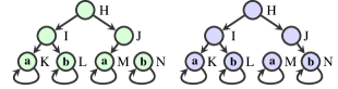
Figure 6: Incremental labeling—Initial (left), Final (right)

Re-labeling states.

Let $\mathit{ancestors}_{K}(V)$ be the ancestors of $V$ in $K$—i.e., a set of vertices s.t. $\mathit{ancestors}_{K}(V)\subseteq Q$ and $q\in\mathit{ancestors}_{K}(V)$, if some node $v\in V$ is reachable from $q$. To define incremental model checking for $\varphi$, we need a function accepting a property $\varphi$, set of vertices $V$, labeling $\mathit{labGr}_{K}$ that is correct for $K$ with respect to $\varphi$ and $Q\setminus\mathit{ancestors}_{K}(V)$, and returns a correct labeling of $K$ with respect to $\varphi$ and $Q$. This function is:

$$\begin{array}[]{l}\mathit{relbl}_{K}(\varphi,\mathit{labGr}_{K},V)=\begin{cases}\mathit{labGr}_{K}&\text{if}~{}V=\emptyset\\ \mathit{relbl}_{K}(\varphi,\mathit{labGr}^{\prime}_{K},V^{\prime})&\text{otherwise}\end{cases}\end{array}$$

where $\mathit{labGr}^{\prime}_{K}(v)$ is $\mathit{labelNode}_{K}(\varphi,v,\mathit{labGr}_{K})$ if $v\in V$, and it is $\mathit{labGr}_{K}(v)$ if $v\not\in V$. The set $V^{\prime}$ is $\{q\mid\exists v\in V:v\in\mathit{succ}_{K}(q)\}$.

Theorem 3.

Let $V\subseteq Q$ be a set of vertices and $\mathit{labGr}_{K}$ a correct labeling with respect to $\varphi$ and $Q\setminus\mathit{ancestors}_{K}(V)$. Then $\mathit{relbl}_{K}(\varphi,\mathit{labGr}_{K},V)$ is a correct labeling w.r.t. $\varphi$ and $Q$.

Given a labeling that is correct with respect to $\varphi$ and $Q$, it is easy to check whether $\varphi$ is true for all the traces starting in the initial states: the predicate $\mathit{checkInitStates}_{K}(\mathit{labGr}_{K},\varphi)$ is defined as $\forall q_{0}\in Q_{0},M\in\mathit{labGr}_{K}(q_{0}):\varphi\in M$. Next, let $Q_{f}$ be the set of all sink states of $K$. Then $\mathit{ancestors}_{K}(Q_{f})$ is the set $Q$ of all states $K$. Therefore, for any initial labeling $\mathit{labGr}_{K}^{0}$, $\mathit{relbl}(\varphi,\mathit{labGr}_{K}^{0},Q_{f})$ is a correct labeling with respect to $\varphi$ and $Q$. The function $\mathit{modelCheck}_{K}(\varphi)$ is defined to be equal to $\mathit{checkInitStates}_{K}(\mathit{relbl}_{K}(\varphi,\mathit{labGr}^{0}_{K},Q_{f}),\varphi)$, where we can set $\mathit{labGr}^{0}_{K}$ to be the empty labeling $\lambda v.\emptyset$.

We now define our incremental model checking function. Let $(K,K^{\prime},U)$ be an update, and $\mathit{labGr}_{K}$ a previously-computed correct labeling of $K$ with respect to $\varphi$ and $Q$, where $Q$ is the set of states of $K$. The function $\mathit{incrModelCheck}(K,\varphi,U,\mathit{labGr}_{K})$ is defined as $\mathit{checkInitStates}_{K^{\prime}}(\mathit{relbl}_{K^{\prime}}(\varphi,\mathit{labGr}_{K},U),\varphi)$. The following shows the correctness of our model checking functions (proof of this and the previous theorem are in Appendix C).

Corollary 1.

First, $\mathit{modelCheck}_{K}(\varphi)=true\iff K\models\varphi$. Second, for $(K,K^{\prime},U)$ and $\mathit{labGr}_{K}$ as above, we have $\mathit{incrModelCheck}(K,\varphi,U,\mathit{labGr}_{K})=\mathit{true}\iff K\models\varphi$.

The runtime complexity of the $\mathit{modelCheck}_{K}$ function is $O(|K|\times 2^{|\varphi|})$. The runtime complexity of the $\mathit{incrModelCheck}$ function is $O(|\mathit{ancestors}_{K}(U)|\times 2^{|\varphi|})$, where $U$ is the set of nodes being updated.

Counterexamples.

This incremental algorithm can generate counterexamples in cases where the formula does not hold. A formula $\neg\varphi$ does not hold if an initial state is labeled by $L$, such that there exists a set $M\in L$, such that $\neg\varphi\in M$. Examining the definition of $\mathit{labelNode}_{K}$, we find that in order to add a set $M$ to the label $L$ of a node $q$, there is a set $M^{\prime}$ in the label of one a child $q^{\prime}$ of $q$ that explains why $M$ is in $L$. The first node of the counterexample trace starting from $q$ is one such child $q^{\prime}$.

6 Implementation and Experiments

We have built a prototype tool that implements the algorithms described in this paper. It consists of 7K lines of OCaml code. The system works by building a Kripke structure (§3) and then repeatedly interacting with a model checker to synthesize an update. We currently provide four checker backends: Incremental uses incremental relabeling to check and recheck formulas, Batch re-labels the entire graph on each call, NuSMV queries a state-of-the-art symbolic model checker in batch mode, and NetPlumber queries an incremental network model checker Kazemian et al. [2013]. All tools except NetPlumber provide counterexample traces, so our system learns from counterexamples whenever possible (§4).

Experiments.

To evaluate performance, we generated configurations for a variety of real-world topologies and ran experiments in which we measured the amount of time needed to synthesize an update (or discover that no order update exists). These experiments were designed to answer two key questions: (1) how the performance of our Incremental checker compares to state-of-the-art tools (NuSMV and NetPlumber), and (2) whether our synthesizer scales to large topologies. We used the Topology Zoo Knight et al. [2011] dataset, which consists of $261$ actual wide-area topologies, as well as synthetically constructed Small-World Newman et al. [2001] and FatTree Al-Fares et al. [2008] topologies. We ran the experiments on a 64-bit Ubuntu machine with 20GB RAM and a quad-core Intel i5-4570 CPU (3.2 GHz) and imposed a 10-minute timeout for each run. We ignored runs in which the solver died due to an out-of-memory error or timeout—these are infrequent (less than 8% of the 996 runs for Figure 7), and our Incremental solver only died in instances where other solvers did too.

Configurations and properties.

A recent paper Liu et al. [2013] surveyed data-center operators to discover common update scenarios, which mostly involve taking switches on/off-line and migrating traffic between switches/hosts. We designed experiments around a similar scenario. To create configurations, we connected random pairs of nodes $(s,d)$ via disjoint initial/final paths $W_{i},W_{f}$, forming a “diamond”, and asserted one of the following properties for each pair:

• Reachability: traffic from a given source must reach a certain destination: $(\mathrm{port}=s)\Rightarrow\mathrm{F\,}(\mathrm{port}=d)$

• Waypointing: traffic must traverse a waypoint $w$:
  $(\mathrm{port}{=}s)\Rightarrow\big{(}(\mathrm{port}{\not=}d)\mathrm{\,U\,}((\mathrm{port}{=}w)\land\mathrm{F\,}(port{=}d))\big{)}$

• Service chaining: traffic must waypoint through several intermediate nodes: $(\mathrm{port}=s)\Rightarrow way(W,d)$, where
  

  $$\begin{array}[]{rcl}way([\,],d)&\equiv&\mathrm{F\,}(\mathrm{port}=d)\\ way(w_{i}::W,d)&\equiv&\big{(}(\bigwedge_{w_{k}\in W}\mathrm{port}{\not=}w_{k}\,\land\,\mathrm{port}{\not=}d)\\ &&\ \mathrm{\,U\,}((\mathrm{port}=w_{i})\land way(W,d))\big{)}.\end{array}$$

Incremental vs. NuSMV/Batch.

Figure 7 (a-c) compares the performance of Incremental and NuSMV backends for the reachability property. Of the 247 Topology Zoo inputs that completed successfully, our tool solved all of them faster. The measured speedups were large, with a geometric mean of $447.23$x. For the 24 FatTree examples, the mean speedup was $465.03$x, and for the 25 Small-World examples, the mean speedup was $4484.73$x. We also compared the Incremental and Batch solvers on the same inputs. Incremental performs better on almost all examples, with mean speedup of $4.26$x, $5.27$x, $11.74$x on the datasets shown in Figure 7(a-c) and maximum runtimes of $0.36$s, $2.80$s, and $0.92$s respectively. The maximum runtimes for Batch were $6.71$s, $39.75$s, and $12.50$s.

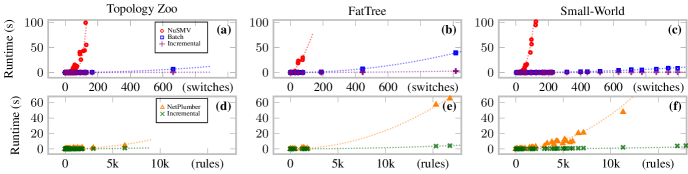
Figure 7: Relative performance results: (a-c) Performance of Incremental vs. NuSMV, Batch, NetPlumber solvers on Topology Zoo, FatTree, Small-World topologies (columns); (d-f) Performance of Incremental vs. NetPlumber (rule-granularity).

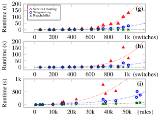
Figure 8: (g) Scalability of Incremental on Small-World topologies of increasing size; (h) Scalability when no correct switch-granularity update exists (i.e. algorithm reports “impossible”), and (i) Scalability of fine-grained (rule-granularity) approach for solving switch-impossible examples in (h).

Incremental vs. NetPlumber.

We also measured the performance of Incremental versus the network property checker NetPlumber (Figure 7(d-f)). Note that NetPlumber uses rule-granularity for updates, so we enabled this mode in our tool for these experiments. For the three datasets, our checker is faster on all experiments, with mean speedups of ($6.41$x, $4.90$x, $17.19$x). NetPlumber does not report counterexamples, putting it at a disadvantage in this end-to-end comparison, so we also measured total Incremental versus NetPlumber runtime on the same set of model-checking questions posed by Incremental for the Small-World example. Our tool is still faster on all instances, with a mean speedup of $2.74$x.

Scalability.

To quantify our tool’s scalability, we constructed Small World topologies with up to 1500 switches, and ran experiments with large diamond updates—the largest has $1015$ switches updating. The results appear in Figure 8(g). The maximum synthesis times for the three properties were $129.04$s, $30.11$s, and $0.85$s, which shows that our tool scales to problems of realistic size.

Infeasible Updates.

We also considered examples for which there is no switch-granular update. Figure 8(h) shows the results of experiments where we generated a second diamond atop the first one, requiring it to route traffic in the opposite direction. Using switch-granularity, the inputs are reported as unsolvable in maximum time $153.48$s, $33.48$s, and $0.69$s. Using rule-granularity, these inputs are solved successfully for up to 1000 switches with maximum times of $776.13$s, $512.84$s, and $82.00$s (see Figure 8(i)).

Waits.

We also separately measured the time needed to run the wait-removal heuristic for the Figure 8 experiments. For (g), the maximum wait-removal runtime was $0.89$s, resulting in $2$ needed waits for each instance. For (i), the maximum wait-removal runtime was $103.87$s, resulting in about $2.6$ waits on average (with a maximum of $4$). For the largest problems in (g) and (i), this corresponds to removal of $1397/1399$ and $55823/55826$ waits (about 99.9%).

7 Related Work

This paper extends preliminary work reported in a workshop paper Noyes et al. [2013]. We present a more precise and realistic network model, and replace expensive calls to an external model checker with calls to a new built-in incremental network model checker. We extend the DFS search procedure with optimizations and heuristics that improve performance dramatically. Finally, we evaluate our tool on a comprehensive set of benchmarks with real-world topologies.

Synthesis of concurrent programs.

There is much previous work on synthesis for concurrent programs Vechev et al. [2010]; Solar-Lezama et al. [2008]; Hawkins et al. [2012]. In particular, work by Solar-Lezama et al. Solar-Lezama et al. [2008] and Vechev et al. Vechev et al. [2010] synthesizes sequences of instructions. However, traditional synthesis and synthesis for networking are quite different. First, traditional synthesis is a game against the environment which (in the concurrent programming case) provides inputs and schedules threads; in contrast, our synthesis problem involves reachability on the space of configurations. Second, our space of configurations is very rich, meaning that checking configurations is itself a model checking problem.

Network updates.

There are many protocol- and property-specific algorithms for implementing network updates, e.g. avoiding packet/bandwidth loss during planned maintenance to BGP Francois et al. [2007]; Raza et al. [2011]. Other work avoids routing loops and blackholes during IGP migration Vanbever et al. [2011]. Work on network updates in SDN proposed the notion of consistent updates and several implementation mechanisms, including two-phase updates Reitblatt et al. [2012]. Other work explores propagating updates incrementally, reducing the space overhead on switches Katta et al. [2013]. As mentioned in Section 2, recent work proposes ordering updates for specific properties Jin et al. [2014], whereas we can handle combinations and variants of these properties. Furthermore, SWAN and zUpdate add support for bandwidth guarantees Hong et al. [2012]; Liu et al. [2013]. Zhou et al. Zhou et al. [2015] consider customizable trace properties, and propose a dynamic algorithm to find order updates. This solution can take into account unpredictable delays caused by switch updates. However, it may not always find a solution, even if one exists. In contrast, we obtain a completeness guarantee for our static algorithm. Ludwig et al. Ludwig et al. [2014] consider ordering updates for waypointing properties.

Model checking.

Model checking has been used for network verification Al-Shaer and Al-Haj [2010]; Mai et al. [2011]; Kazemian et al. [2012]; Khurshid et al. [2012]; Majumdar et al. [2014]. The closest to our work is the incremental checker NetPlumber Kazemian et al. [2013]. Surface-level differences include the specification languages (LTL vs. regular expressions), and NetPlumber’s lack of counterexample output. The main difference is incrementality: Netplumber restricts checking to “probe nodes,” keeping track of “header-space” reachability information for those nodes, and then performing property queries based on this. In contrast, we look at the property, keeping track of portions of the property holding at each node, which keeps incremental rechecking times low. The empirical comparison (Section 6) showed better performance of our tool as a back-end for synthesis.

Incremental model checking has been studied previously, with Sokolsky and Smolka [1994] presenting the first incremental model checking algorithm, for alternation-free $\mu$-calculus. We consider LTL properties and specialize our algorithm to exploit the no-forwarding-loops assumption. The paper Chockler et al. [2011] introduced an incremental algorithm, but it is specific to the type of partial results produced by IC3 Bradley [2011].

8 Conclusion

We present a practical tool for automatically synthesizing correct network update sequences from formal specifications. We discuss an efficient incremental model checker that performs orders of magnitude better than state-of-the-art monolithic tools. Experiments on real-world topologies demonstrate the effectiveness of our approach for synthesis. In future work, we plan to explore both extensions to deal with network failures and bandwidth constraints, and deeper foundations of techniques for network updates.

The authors would like to thank the PLDI reviewers and AEC members for their insightful feedback on the paper and artifact, as well as Xin Jin, Dexter Kozen, Mark Reitblatt, and Jennifer Rexford for helpful comments. Andrew Noyes and Todd Warszawski contributed a number of early ideas through an undergraduate research project. This work was supported by the NSF under awards CCF-1421752, CCF-1422046, CCF-1253165, CNS-1413972, CCF-1444781, and CNS-1111698; the ONR under Award N00014-12-1-0757; and gifts from Fujitsu Labs and Intel.

Appendix A Network Model Auxiliary Definitions

We first define what it means for a table to be active, i.e. the controller contains an update that will eventually produce that table.

Definition 6 (Active Forwarding Table).

Let $N$ be a network. The forwarding table $\mathit{tbl}$ is active in the epoch $\mathit{ep}$ for the switch $\mathit{sw}$ if

1. $\mathit{ep}=0$ and $\mathit{tbl}$ is the initial table of $\mathit{sw}$ in $N$, or

2. $\mathit{ep}>0$ and either (a) if there exists a command $(\mathit{sw}^{\prime},\mathit{tbl}^{\prime})\in C.\mathit{cmds}$ such that $\mathit{sw}=\mathit{sw}^{\prime}$ and the number of $\mathit{wait}$ commands preceding $(\mathit{sw},\mathit{tbl})$ in $C.\mathit{cmds}$ is $\mathit{ep}$, then $\mathit{tbl}=\mathit{tbl}^{\prime}$, or (b) if there does not exist such a command, then $\mathit{tbl}$ is the table active for the switch $\mathit{sw}$ in epoch $\mathit{ep}-1$.

Next we define what it means for an observation $o^{\prime}$ to succeed $o$.

Definition 7 (Successor Observation).

Let $N$ be a network and let $o=(\mathit{sw},\mathit{pt},\mathit{pkt})$ and $o^{\prime}=(\mathit{sw}^{\prime},\mathit{pt}^{\prime},\mathit{pkt}^{\prime})$ be observations. The observation $o^{\prime}$ is a successor of $o$ in $\mathit{ep}$, written $o\overset{\mathit{ep}}{\sqsubseteq}o^{\prime}$, if either:

• there exists a switch $S_{i}$ and link $L_{j}$ such that $S_{i}.\mathit{sw}=\mathit{sw}$ and $S_{i}.\mathit{tbl}$ is active in $\mathit{ep}$ and $L_{j}.\mathit{loc}=(\mathit{sw},\mathit{pt}_{j})$ and $L_{j}.\mathit{loc}^{\prime}=(\mathit{sw}^{\prime},\mathit{pt}^{\prime})$ and $(\mathit{pt}_{j},\mathit{pkt}^{\prime})\in[\![S_{i}.\mathit{tbl}]\!](\mathit{pt},\mathit{pkt})$, or

• there exists a switch $S_{i}$, a link $L_{j}$, and a host $\mathit{h}$ such that $S_{i}.\mathit{sw}=\mathit{sw}$ and $S_{i}.\mathit{tbl}$ is active in $\mathit{ep}$ and $L_{j}.\mathit{loc}=(\mathit{sw},\mathit{pt}^{\prime})$ and $L_{j}.\mathit{loc}^{\prime}=\mathit{h}$ and $(\mathit{pt}^{\prime},\mathit{pkt}^{\prime})\in[\![S_{i}.\mathit{tbl}]\!](\mathit{pt},\mathit{pkt})$.

Intuitively $o\overset{\mathit{ep}}{\sqsubseteq}o^{\prime}$ if the packet in $o$ could have directly produced the packet in $o^{\prime}$ in $\mathit{ep}$ by being processed on some switch. The two cases correspond to an internal and egress processing steps.

Definition 8 (Unconstrained Single-Packet Trace).

Let $N$ be a network. The sequence $(o_{1}\cdots o_{l})$ is a unconstrained single-packet trace of $N$ if $N\xrightarrow{o_{1}^{\prime}}\dots\xrightarrow{o_{k}^{\prime}}N_{k}$ such that $(o_{1}\cdots o_{l})$ is a subsequence of $(o_{1}^{\prime}\cdots o_{k}^{\prime})$ for which

• every observation is a successor of the preceding observation in monotonically increasing epochs, and

• if $o_{1}=o_{j}^{\prime}=(\mathit{sw},\mathit{pt},\mathit{pkt})$, i.e. $N\xrightarrow{o_{1}^{\prime}}\dots\xrightarrow{o_{j}^{\prime}=o_{1}}N_{j}\xrightarrow{o_{j+1}^{\prime}}\dots\xrightarrow{o_{k}^{\prime}}N_{k}$, then no $o_{i}^{\prime}\in\{o_{1}^{\prime},\cdots,o_{j-1}^{\prime}\}$ precedes $o_{1}$, and

• the $o_{l}$ transition is an Out terminating at a host.

Unconstrained single-packet traces are not required to begin at a host. We write $\mathrm{bar}{\mathcal{T}}(N)$ for the set of unconstrained single-packet traces generated by $N$, and note that $\mathcal{T}(N)\subseteq\mathrm{bar}{\mathcal{T}}(N)$.

Definition 9 (Network Kripke Structure).

Let $N$ be a static network. We define a Kripke structure $\mathcal{K}(N)=(Q,Q_{0},\delta,\lambda)$ as follows. The set of states $Q$ comprises tuples of the form $(\mathit{sw},\mathit{pt},T_{k})$. The set $Q_{0}$ contains states $(\mathit{sw},\mathit{pt},T_{k})$ where $\mathit{sw}$ and $\mathit{pt}$ are adjacent to an ingress link—i.e., there exists a link $L_{j}$ and host $\mathit{h}$ such that $L_{j}.\mathit{loc}=\mathit{h}$ and $L_{j}.\mathit{loc}^{\prime}=(\mathit{sw},\mathit{pt})$. Transition relation $\delta$ contains all pairs of states $(\mathit{sw},\mathit{pt},T_{k})$ and $(\mathit{sw}^{\prime},\mathit{pt}^{\prime},T_{k}^{\prime})$ where there exists a switch $S$ and a link $L$ such that $S.\mathit{sw}=\mathit{sw}$ and either:

• there exists a link $L_{j}$ and packets $\mathit{pkt}\in T_{k}$ and $\mathit{pkt}^{\prime}\in T_{k}^{\prime}$ such that $L.\mathit{loc}^{\prime}=(\mathit{sw},pt)$ and $L_{j}.\mathit{loc}=(\mathit{sw},\mathit{pt}_{j})$ and $L_{j}.\mathit{loc}^{\prime}=(\mathit{sw}^{\prime},\mathit{pt}^{\prime})$ and $(\mathit{pkt}^{\prime},\mathit{pt}_{j})\in[\![S.\mathit{tbl}]\!](\mathit{pkt},\mathit{pt})$.

• there exists a link $L_{j}$, a host $\mathit{h}$, and packets $\mathit{pkt}\in T_{k}$ and $\mathit{pkt}^{\prime}\in T_{k}^{\prime}$ such that $L.\mathit{loc}^{\prime}=(\mathit{sw},pt)$ and $L_{j}.\mathit{loc}=(\mathit{sw},\mathit{pt}^{\prime})$ and $L_{j}.\mathit{loc}^{\prime}=\mathit{h}$ and $(\mathit{pkt}^{\prime},\mathit{pt}^{\prime})\in[\![S.\mathit{tbl}]\!](\mathit{pkt},\mathit{pt})$.

• $(\mathit{sw},\mathit{pt},T_{k})=(\mathit{sw}^{\prime},\mathit{pt}^{\prime},T_{k}^{\prime})$ and there exists a packet $\mathit{pkt}\in T_{k}$ such that $L.\mathit{loc}^{\prime}=(\mathit{sw},pt)$ and $[\![S.\mathit{tbl}]\!](\mathit{pkt},\mathit{pt})=\{\}$.

• $(\mathit{sw},\mathit{pt},T_{k})=(\mathit{sw}^{\prime},\mathit{pt}^{\prime},T_{k}^{\prime})$ and there exists a link $L_{j}$ and host $\mathit{h}$ such that $L_{j}.\mathit{loc}=(\mathit{sw},\mathit{pt})$ and $L_{j}.\mathit{loc}^{\prime}=\mathit{h}$.

Finally, the labeling function $\lambda$ maps each state $(\mathit{sw},\mathit{pt},T_{k})$ to $T_{k}$, which captures the set of all possible header values of packets located at switch $\mathit{sw}$ and port $\mathit{pt}$.

The four cases of the $\delta$ relation correspond to forwarding packets to an internal link, forwarding packets out an egress, dropping packets on a switch, or reaching an egress (inducing a self-loop).

We can relate the observations generated by a network $N$ and the traces of the Kripke structure generated from it.

Definition 10 (Trace Relation).

Let $N$ be a static network and $K$ a Kripke structure. Let $\lesssim$ be a relation on observations of $N$ and states of $K$ defined by $(\mathit{sw},\mathit{pt},\mathit{pkt})~{}\lesssim~{}(\mathit{sw},\mathit{pt},T_{k})$ if and only if $\mathit{pkt}\in T_{k}$. Lift $\lesssim$ to a relation on (finite) sequences of observations and (infinite) traces by repeating the final observation and requiring $\lesssim$ to hold pointwise: $o_{1}\cdots o_{k}~{}\lesssim~{}t$ if and only if $o_{i}~{}\lesssim~{}t_{i}$ for $i$ from $1$ to $k$ and $o_{k}~{}\lesssim~{}t_{j}$ for all $j>k$.

Lemma 4 (Traces of a Stable Network).

Let $N$ be a stable network. Then for each trace $t\in\mathrm{bar}{\mathcal{T}}(N)$, there exists a trace $t^{\prime}\in\mathcal{T}(N)$ such that $t$ is a suffix of $t^{\prime}$.

Lemma 5 (Trace-Equivalence).

Let $N_{1},N_{n}$ be static networks where $N_{1}\rightarrow\cdots\rightarrow N_{n}$ and no transition is an update command. For a single-packet trace $t$, we have $t\in\mathcal{T}(N_{1})\iff t\in\mathcal{T}(N_{n})$.

Lemma 6 (Induced Sequence of Networks).

Let $N_{1}$ be a static network, and let $N_{1}^{\prime}$ be the network obtained by emptying all packets from $N_{1}$. Let $\mathit{cmds}$ be a sequence of commands, and let $c_{1}\cdots c_{n-1}$ be the subsequence of update commands. Construct the sequence $N_{1}^{\prime}\rightarrow\cdots\rightarrow N_{n}^{\prime}$ of empty networks by executing the update commands in order. Now, given any sequence $N_{1}\rightarrow\cdots\rightarrow N_{n}$ induced by $\mathit{cmds}$, we have $N_{i}\simeq N_{i}^{\prime}$ for all $i$.

In other words, any induced sequence of static networks is pointwise trace-equivalent to the unique sequence of network configurations generated by running the update commands in order.

Appendix B Synthesis Algorithm Correctness Proofs

Lemma 1 (Network Kripke Structure Soundness).

Let $N$ be a static network and $K=\mathcal{K}(N)$ a network Kripke structure. For every single-packet trace $t$ in $\mathcal{T}(N)$ there exists a trace $t^{\prime}$ of $K$ from a start state such that $t\lesssim t^{\prime}$, and vice versa.

Proof.

We proceed by induction over $k$, the length of the (finite prefix of the) trace. The base case $k=1$ is easy to see, since the lone observation in $t$ must be on an ingress link, meaning the corresponding state in $K$ will be an initial state with a self-loop (case 3 of Definition 9), and these are equivalent via Definition 10.

For the inductive step ($k>1$), we wish to show both directions of subtrace relation $\lesssim$ to conclude equivalence. First, let $t=o_{1},\cdots,o_{k+1}$ be a single-packet trace of length $k+1$ in $\mathcal{T}(N)$, and we must show that $\exists t^{\prime}\in\mathcal{K}(N)$ such that $t\lesssim t^{\prime}$. Let $t^{k}$ be the prefix of $t$ having length $k$. By our induction hypothesis, there exists $t^{\prime k}=s_{1},\cdots,s_{k-1},s_{k},s_{k},\cdots\in\mathcal{K}(N)$ such that $t^{k}\lesssim t^{\prime k}$. We have the successor relation $o_{k}\sqsubseteq o_{k+1}$, so Definition 7 and 9 tells us that we have a transition $s_{k}\rightarrow s^{\prime}$ for some $s^{\prime}\in K$. We see that this $s^{\prime}$ is exactly what we need to construct $t^{\prime}=s_{1},\cdots,s_{k},s^{\prime},s^{\prime},\cdots$ which satisfies the relation $t\lesssim t^{\prime}$.

Now, let $t^{\prime}=s_{1},\cdots,s_{k},s_{k+1},s_{k+1},\cdots$ be a trace in $\mathcal{K}(N)$ for which the finite prefix has length $k+1$. We must show that $\exists t\in\mathcal{T}(N)$ such that $t\lesssim t^{\prime}$. Let $t^{\prime k}=s_{1},\cdots,s_{k-1},s_{k},s_{k},\cdots$, and by our induction hypothesis, and there exists $t^{k}=o_{1},\cdots,o_{k}$ such that $t^{k}\lesssim t^{\prime k}$. Consider transition $s_{k}\rightarrow s_{k+1}$. If $s_{k}=s_{k+1}$, then $t^{\prime}=t^{\prime k}$, so we can let $t=t^{k}$, and conclude that $t\lesssim t^{\prime}$. Otherwise, if $s_{k}\not=s_{k+1}$, then we have one of the first two cases in Definition 9, which correspond to the cases in Definition 7, allowing us to construct an $o_{k+1}$ such that $o_{k}\sqsubseteq o_{k+1}$. We let $t=o_{1},\cdots,o_{k},o_{k+1}$, and conclude that $t\lesssim t^{\prime}$. ∎

We want to develop a lemma showing that the correctness of careful command sequences can be reduced to the correctness of each induced $N_{i}$, so we start with the following auxiliary lemma:

Lemma 7 (Traces of a Careful Network).

Let $N$ be a stable network with $C.\mathit{cmds}$ careful, and consider a sequence of static networks induced by $C.\mathit{cmds}$. For every trace $t\in\mathcal{T}(N)$ there exists a stable static network $N_{i}$ in the sequence s.t. $t\in\mathcal{T}(N_{i})$.

Proof.

I. First, we show that at most one update transition can be involved in the trace. In other words, if $N\xrightarrow{o_{1}^{\prime}}\dots\xrightarrow{o_{k}^{\prime}}N_{k}$ where $t=o_{1}\cdots o_{n}$ is a subsequence of $o_{1}^{\prime}\cdots o_{k}^{\prime}$, and if $f:\mathbb{N}\rightarrow\mathbb{N}$ is a bijection between $o_{i}$ indices and $o_{i}^{\prime}$ indices, then at most one of the transitions $o_{f(1)}^{\prime},\cdots,o_{f(n)}^{\prime}$ is an Update transition.

Assume to the contrary that there are more than one such transitions, and consider two of them, $o_{i}^{\prime},o_{j}^{\prime}$ where $i,j\in\{f(1),\cdots,f(n)\}$, assuming without loss of generality that $i<j$. Now, since the sequence $C.cmds$ is careful, we must have both an Incr and Flush transition between $o_{i}^{\prime}$ and $o_{j}^{\prime}$. This means that the second update $o_{j}^{\prime}$ cannot happen while the trace’s packet is still in the network, i.e. $j>f(n)$, and we have reached a contradiction.

II. Now, if there are zero update transitions, we are done, since the trace is contained in the first static $N$. If there is one update transition $N_{k+1}=N_{k}[\mathit{sw}\leftarrow\mathit{tbl}]$, and this update occurs before the packet reaches $\mathit{sw}$ in the trace, then the trace is fully contained in $N_{k+1}$. Otherwise, the trace is fully contained in $N_{k}$. ∎

Lemma 2 (Careful Correctness).

Let $N$ be a stable network with $C.\mathit{cmds}$ careful and let $\varphi$ be an LTL formula. If $\mathit{cmds}$ is careful and $N_{i}\models\phi$ for each static network in any sequence induced by $\mathit{cmds}$, then $\mathit{cmds}$ is correct with respect to $\varphi$.

Proof.

Consider a trace $t\in\mathcal{T}(N)$. From Lemma 7, we have $t\in\mathcal{T}(N_{i})$ for some $N_{i}$ in the induced sequence. Thus $t\models\varphi$, since our hypothesis tells us that $N_{i}\models\varphi$. Since this is true for an arbitrary trace, we have shown that $\mathcal{T}(N)\models\varphi$, i.e. $N\models\varphi$, meaning that $\mathit{cmds}$ is correct with respect to $\varphi$. ∎

Theorem 1 (Soundness).

Given initial network $\mathit{N}_{i}$, final configuration $\mathit{N}_{f}$, and LTL formula $\varphi$, if OrderUpdate returns a command sequence $\mathit{cmds}$, then ${\mathit{N}_{i}\overset{\mathit{cmds}}{\longrightarrow}\mathit{N}^{\prime}}$ s.t. $\mathit{N}^{\prime}\simeq\mathit{N}_{f}$, and $\mathit{cmds}$ is correct with respect to $\varphi$ and $\mathit{N}_{i}$.

Proof.

It is easy to show that if OrderUpdate returns $\mathit{cmds}$, then ${\mathit{N}_{i}\overset{\mathit{cmds}}{\longrightarrow}\mathit{N}^{\prime}}$ where $\mathit{N}^{\prime}\simeq\mathit{N}_{f}$. Each update in the returned sequence changes a switch configuration of one switch $s$ to the configuration $\mathit{N}_{f}(s)$, and the algorithm terminates when all (and only) switches $s$ such that $\mathit{N}_{i}(s)\neq\mathit{N}_{f}(s)$ have been updated.

Observe that if OrderUpdate returns $\mathit{cmds}$, the sequence can be made careful by choosing an adequate time delay between each update command, and for all $j\in\{0,\cdots,n\}$, $\mathit{N}_{j}\models\varphi$. This is ensured by the call to a model checker (Line 10). We use Lemma 2 to conclude that $\mathit{cmds}$ is correct with respect to $\varphi$ and $\mathit{N}_{i}$. ∎

To show that OrderUpdate is complete with respect to simple and careful command sequences, we observe that OrderUpdate searches through all simple and careful sequences.

Theorem 2 (Completeness).

Given initial network $\mathit{N}_{i}$, final configuration $\mathit{N}_{f}$, and specification $\varphi$, if there exists a simple, careful sequence $\mathit{cmds}$ with ${\mathit{N}_{i}\overset{\mathit{cmds}}{\longrightarrow}\mathit{N}^{\prime}}$ s.t. $\mathit{N}^{\prime}\simeq\mathit{N}_{f}$, then OrderUpdate returns one such sequence.

Appendix C Incremental Checking Correctness Proofs

Lemma 3.

First, $\mathit{HoldsSink}(q,M)\Leftrightarrow\exists t\in\mathit{traces}(q):t\models M$ for sink states $q$. Second, if $\mathit{labGr}_{K}$ is a correct labeling with respect to $\varphi$ and $\mathit{succ}_{K}(q)$, then $\mathit{Holds}_{K}(q,M,\mathit{labGr}_{K})\Longleftrightarrow\exists t\in\mathit{traces}_{K}(q):t\models M$.

Proof.

First, for sink states, observe that there is a unique trace $t$ in $\mathit{traces}(q)$, as $q$ is a sink state. We first prove that $t\models\varphi$ iff $\mathit{Holds_{0}}(q,\varphi)$. We prove this by induction on the structure of the LTL formula. Then we observe that there is a unique maximally-consistent set $M$ such that $t\models M$. This is the set $\{\psi\mid t\models\psi\wedge\psi\in\mathit{ecl}(\varphi)\}$. We then use the definition of $\mathit{HoldsSink}(q,M)$ for sink states to conclude the proof.

Now consider non-sink states: we first prove soundness, i.e., if $\mathit{Holds}_{K}(q,M,\mathit{labGr}_{K})$, then there exists $t\in traces(q)$ such that $t\models M$. We have $\mathit{Holds}_{K}(q,M,\mathit{labGr}_{K})$ iff $(\lambda(q)=(\mathit{AP}\cap M))$ and there exists $q^{\prime}\in\mathit{succ}_{K}(M)$, and $M^{\prime}\in\mathit{labGr}_{K}(q^{\prime})$ such that $\mathit{follows}(M,M^{\prime})$. By assumption of the theorem, we have that if $M^{\prime}\in\mathit{labGr}_{K}(q^{\prime})$, then there exists a trace $t^{\prime}$ in $\mathit{traces}(q^{\prime})$ such that $t^{\prime}\models M^{\prime}$. Consider a trace $t$ such that $t_{0}=q$ and $t^{1}=t^{\prime}$. For each $\psi\in M$, we can prove that $t\models\psi$ as follows. The base case of the proof by induction is implied by the fact that $q\models(\mathit{AP}\cap M)$. The inductive cases are proven using the definitions of maximally-consistent set and the function $\mathit{follows}$. We now prove completeness, i.e., that if there exists a trace $t$ in $\mathit{traces}_{K}(q)$ such that $t\models M$, then $\mathit{Holds}_{K}(q,M,\mathit{labGr}_{K})$ is true. Let $t$ be the trace $qq_{1}q_{2}\ldots$. It is easy to see that if $M$ is a maximally-consistent set, and $t\models M$, then $M=\{\psi\mid\psi\in\mathit{ecl}(\varphi)\wedge t\models\psi\}$. Let us consider the set of formulas $S=\{\psi\mid\psi\in\mathit{ecl}(\varphi)\wedge t^{1}\models\psi\}$. Observe that $S$ is a maximally-consistent set. By assumption of the theorem, we have that $S$ is in $\mathit{labGr}_{K}(q_{1})$. It is easy to verify that $\mathit{follows}(M,S)$. ∎

Theorem 3.

Let $V\subseteq Q$ be a set of vertices and $\mathit{labGr}_{K}$ a correct labeling with respect to $\varphi$ and $Q\setminus\mathit{ancestors}_{K}(V)$. Then $\mathit{relbl}_{K}(\varphi,\mathit{labGr}_{K},V)$ is a correct labeling w.r.t. $\varphi$ and $Q$.

Proof.

We first note that only ancestors of nodes in $V$ are re-labeled—all the other nodes are correctly labeled by assumption on $\mathit{labGr}$. We say that a node $q$ is at level $k$ w.r.t. a set of vertices $T$ iff the longest simple path from $q$ to a node in $T$ is $k$. Let $H_{k}$ be the set of nodes at level $k$ from $V$. We prove by induction on $k$ that at $k$-th iteration, we have a correct labeling of $K$ w.r.t. $\varphi$ and $(S\setminus\mathit{ancestors}_{K}(V))\cup H_{k}$, where $S$ is the set of states of $K$. We can prove the inductive claim using Lemma 3. ∎

Corollary 1.

First, $\mathit{modelCheck}_{K}(\varphi)=true\iff K\models\varphi$. Second, for $(K,K^{\prime},U)$ and $\mathit{labGr}_{K}$ as above, we have $\mathit{incrModelCheck}(K,\varphi,U,\mathit{labGr}_{K})=\mathit{true}\iff K\models\varphi$.

Proof.

Using Theorem 3, and the fact that the set $\mathit{ancestors}_{K}(S_{f})$ is the set $S$ of all states $K$, we obtain that $\mathit{labGr}_{K}=\mathit{relbl}_{K}(\varphi,\mathit{labGr}_{K}^{0},S_{f})$ is a correct labeling of $K$ with respect to $\varphi$ and $S$. In particular, for all initial states $q_{0}$, we have that for all $M\subset\mathit{ecl}(\varphi)$, $m\in\mathit{labGr}_{K}(q_{0})$ iff there exists a trace $t\in\mathit{traces}_{K}(q_{0})$ such that $t\models M$. We now use the definition of $\mathit{checkInitStates}$ to show that if $\mathit{checkInitStates}$ returns true, then there is no initial state $q_{0}$ such that there exists $M\in\mathit{labGr}_{K}(q_{0})$ such that $\neg\varphi\in M$. Thus for all initial states $q_{0}$, for all traces $t$ in $\mathit{traces}(t_{0})$, we have that $t\models\varphi$.

The proof for incremental model checking is similar. ∎

References

- Al-Fares et al. [2008] M. Al-Fares, A. Loukissas, and A. Vahdat. A Scalable, Commodity Data Center Network Architecture. In SIGCOMM, 2008.
- Al-Shaer and Al-Haj [2010] E. Al-Shaer and S. Al-Haj. FlowChecker: Configuration Analysis and Verification of Federated OpenFlow Infrastructures. In SafeConfig, 2010.
- Alizadeh et al. [2010] M. Alizadeh, A. Greenberg, D. Maltz, J. Padhye, P. Patel, B. Prabhakar, S. Sengupta, and M. Sridharan. Data Center TCP (DCTCP). In SIGCOMM, pages 63–74, 2010.
- Berry and Boudol [1990] G. Berry and G. Boudol. The Chemical Abstract Machine. In POPL, pages 81–94, 1990.
- Bradley [2011] A. Bradley. SAT-Based Model Checking without Unrolling. In VMCAI, 2011.
- Casado et al. [2014] M. Casado, N. Foster, and A. Guha. Abstractions for Software-Defined Networks . CACM, 57(10):86–95, Oct. 2014.
- Chockler et al. [2011] H. Chockler, A. Ivrii, A. Matsliah, S. Moran, and Z. Nevo. Incremental Formal Verification of Hardware. In FMCAD, pages 135–143, 2011.
- Foster et al. [2011] N. Foster, R. Harrison, M. Freedman, C. Monsanto, J. Rexford, A. Story, and D. Walker. Frenetic: A Network Programming Language. In ICFP, pages 279–291, 2011.
- Francois and Bonaventure [2007] P. Francois and O. Bonaventure. Avoiding Transient Loops during the Convergence of Link-state Routing Protocols. IEEE/ACM Transactions on Networking, 15(6):1280–1292, 2007.
- Francois et al. [2007] P. Francois, O. Bonaventure, B. Decraene, and P.-A. Coste. Avoiding Disruptions during Maintenance Operations on BGP Sessions. IEEE Transactions on Network and Service Management, 4(3):1–11, 2007.
- Guha et al. [2013] A. Guha, M. Reitblatt, and N. Foster. Machine-Verified Network Controllers . In PLDI, June 2013.
- Hawkins et al. [2012] P. Hawkins, A. Aiken, K. Fisher, M. Rinard, and M. Sagiv. Concurrent Data Representation Synthesis. In PLDI, pages 417–428, June 2012.
- Hong et al. [2012] C.-Y. Hong, S. Kandula, R. Mahajan, M. Zhang, V. Gill, M. Nanduri, and R. Wattenhofer. Achieving High Utilization with Software-Driven WAN. In SIGCOMM, pages 15–26, Aug. 2012.
- Jain et al. [2013] S. Jain, A. Kumar, S. Mandal, J. Ong, L. Poutievski, A. Singh, S. Venkata, J. Wanderer, J. Zhou, M. Zhu, J. Zolla, U. Hölzle, S. Stuart, and A. Vahdat. B4: Experience with a Globally-deployed Software Defined WAN. In SIGCOMM, 2013.
- Jin et al. [2014] X. Jin, H. Liu, R. Gandhi, S. Kandula, R. Mahajan, M. Zhang, J. Rexford, and R. Wattenhofer. Dynamic Scheduling of Network Updates. In SIGCOMM, pages 539–550, 2014.
- John et al. [2008] J. P. John, E. Katz-Bassett, A. Krishnamurthy, T. Anderson, and A. Venkataramani. Consensus Routing: The Internet as a Distributed System. In NSDI, pages 351–364, 2008.
- Katta et al. [2013] N. P. Katta, J. Rexford, and D. Walker. Incremental Consistent Updates. In HotSDN, pages 49–54. ACM, 2013.
- Kazemian et al. [2012] P. Kazemian, G. Varghese, and N. McKeown. Header Space Analysis: Static Checking for Networks. In NSDI, 2012.
- Kazemian et al. [2013] P. Kazemian, M. Chang, H. Zeng, G. Varghese, N. McKeown, and S. Whyte. Real Time Network Policy Checking Using Header Space Analysis. NSDI, pages 99–112, 2013.
- Khurshid et al. [2012] A. Khurshid, W. Zhou, M. Caesar, and P. Godfrey. VeriFlow: Verifying Network-wide Invariants in Real Time. ACM SIGCOMM CCR, 2012.
- Knight et al. [2011] S. Knight, H. Nguyen, N. Falkner, R. Bowden, and M. Roughan. The Internet Topology Zoo. IEEE Journal on Selected Areas in Communications, 29(9):1765–1775, Oct. 2011.
- Lazaris et al. [2014] A. Lazaris, D. Tahara, X. Huang, L. Li, A. Voellmy, Y. Yang, and M. Yu. Tango: Simplifying SDN Programming with Automatic Switch Behavior Inference, Abstraction, and Optimization. 2014.
- Liu et al. [2013] H. H. Liu, X. Wu, M. Zhang, L. Yuan, R. Wattenhofer, and D. Maltz. zUpdate: Updating Data Center Networks with Zero Loss. In SIGCOMM, pages 411–422. ACM, 2013.
- Ludwig et al. [2014] A. Ludwig, M. Rost, D. Foucard, and S. Schmid. Good Network Updates for Bad Packets: Waypoint Enforcement Beyond Destination-Based Routing Policies. In HotNets, 2014.
- Mahajan and Wattenhofer [2013] R. Mahajan and R. Wattenhofer. On Consistent Updates in Software Defined Networks. In SIGCOMM, Nov. 2013.
- Mai et al. [2011] H. Mai, A. Khurshid, R. Agarwal, M. Caesar, P. Godfrey, and S. T. King. Debugging the Data Plane with Anteater. In SIGCOMM, 2011.
- Majumdar et al. [2014] R. Majumdar, S. Tetali, and Z. Wang. Kuai: A Model Checker for Software-defined Networks. In FMCAD, 2014.
- McKeown et al. [2008] N. McKeown, T. Anderson, H. Balakrishnan, G. Parulkar, L. Peterson, J. Rexford, S. Shenker, and J. Turner. OpenFlow: Enabling Innovation in Campus Networks. ACM SIGCOMM CCR, 2008.
- Newman et al. [2001] M. E. Newman, S. H. Strogatz, and D. J. Watts. Random Graphs with Arbitrary Degree Distributions and their Applications. 2001.
- Noyes et al. [2013] A. Noyes, T. Warszawski, and N. Foster. Toward Synthesis of Network Updates. In SYNT, July 2013.
- Open Networking Foundation [2013] Open Networking Foundation. OpenFlow 1.4 Specification, 2013.
- Raza et al. [2011] S. Raza, Y. Zhu, and C.-N. Chuah. Graceful Network State Migrations. IEEE/ACM Transactions on Networking, 19(4):1097–1110, 2011.
- Reitblatt et al. [2012] M. Reitblatt, N. Foster, J. Rexford, C. Schlesinger, and D. Walker. Abstractions for Network Update. In SIGCOMM, 2012.
- Sokolsky and Smolka [1994] O. Sokolsky and S. Smolka. Incremental Model Checking in the Modal Mu-Calculus. In CAV, pages 351–363, 1994.
- Solar-Lezama et al. [2008] A. Solar-Lezama, C. G. Jones, and R. Bodik. Sketching Concurrent Data Structures. In PLDI, pages 136–148, 2008.
- Vanbever et al. [2011] L. Vanbever, S. Vissicchio, C. Pelsser, P. Francois, and O. Bonaventure. Seamless Network-wide IGP Migrations. In SIGCOMM, 2011.
- Vardi and Wolper [1986] M. Y. Vardi and P. Wolper. An Automata-Theoretic Approach to Automatic Program Verification (Preliminary Report). In LICS, 1986.
- Vechev et al. [2010] M. Vechev, E. Yahav, and G. Yorsh. Abstraction-guided Synthesis of Synchronization. In POPL, pages 327–338, 2010.
- Wolper et al. [1983] P. Wolper, M. Y. Vardi, and A. P. Sistla. Reasoning about Infinite Computation Paths (Extended Abstract). In FOCS, 1983.
- Zhou et al. [2015] W. Zhou, D. Jin, J. Croft, M. Caesar, and B. Godfrey. Enforcing Generalized Consistency Properties in Software-Defined Networks. In NSDI, 2015.