Description of collective and quasiparticle excitations in deformed actinide nuclei:
The first application of the Heavy Shell Model

Abstract

The Heavy Shell Model (HSM) (Y. Sun and C.-L. Wu, Phys. Rev. C 68, 024315 (2003)) was proposed to take the advantages of two existing models, the projected shell model (PSM) and the Fermion Dynamical Symmetry Model (FDSM). To construct HSM, one extends the PSM by adding collective $D$-pairs into the intrinsic basis. The HSM is expected to describe simultaneously low-lying collective and quasi-particle excitations in deformed nuclei, and still keeps the model space tractable even for the heaviest systems. As the first numerical realization of the HSM, we study systematically the band structures for some deformed actinide nuclei, with a model space including up to 4-quasiparticle and 1-$D$-pair configurations. The calculated energy levels for the ground-state bands, the collective bands such as $\beta$- and $\gamma$-bands, and some quasiparticle bands agree well with known experimental data. Some low-lying quasiparticle bands are predicted, awaiting experimental confirmation.

I INTRODUCTION

The interplay between collective motion and quasi-particle excitations has been a long-standing topic in nuclear structure physics. The nuclear shell model is the most fundamental method that treats nuclear systems fully quantum mechanically in terms of nucleons. However, it is difficult for the conventional shell model based on a spherical basis to study heavy, deformed nuclei because of the problem of huge dimensionality. Even with the today’s computer power and novel diagonalization algorithms, a full shell model calculation for an arbitrarily large system seems to be impossible. To overcome the dimensionality problem, one needs to seek judicious truncation schemes and use more efficient shell-model bases. In the literatures, the Projected Shell Model (PSM) Har95 and the Fermion Dynamical Symmetry Model (FDSM) Wu94 are two such examples. Both of them are based on the shell model concept, but are constructed according to different truncation schemes, thus emphasizing different physical aspects.

In the PSM, shell model diagonalization is carried out in the projected deformed basis constructed by choosing a few quasiparticle (qp) orbitals near the Fermi surfaces and performing angular-momentum and particle-number projection on the qp configurations Har95 . In this way, the PSM is able to describe low-lying rotational bands built upon qp excitations. It has been successful for the PSM to study the rotational states in heavy Sun04 and superheavy nuclei Falih09 , as well as the states of super-deformation Sun95 ; Sun97 . Moreover, it has been shown that comparing with the large-scale shell model calculations Cau95 , the PSM can achieve a similar accuracy in describing the deformed ⁴⁸Cr Har09 and the superdeformed ³⁶Ar Lon01 . However, the original version of the PSM was not designed to treat collective vibrational states such as $\beta$- and $\gamma$-vibrations. The lack of ingredients for collective excitations in the PSM makes it difficult to produce these low-lying collective bands, and also limits its applications only to well deformed nuclei. To release the restriction of axial symmetry in the deformed basis, the Triaxial Projected Shell Model (TPSM) was introduced Sheikh99 . A more recent example of the TPSM application is to describe the $\gamma$-vibrational bands in some Er isotopes TPSM .

On the other hand, the Interacting Boson Model (IBM) Iac87 is a successful model for the description of low-lying collective states. In this model, the coherent $S$- and $D$-pairs are assumed to be the building blocks of the low-lying collective states, and are approximated as ${\it s}$ and ${\it d}$ bosons. It has been shown that an axially symmetric rotor possesses the SU(3) symmetry, while a $\gamma$-soft rotor possesses the SO(6) symmetry. The $\beta$- and $\gamma$-vibrations including the scissors mode vibration in deformed nuclei can be classified as different SU(3) or SO(6) irreducible representations Iac84 . Since nucleons are fermions, the later developed FDSM directly uses coherent nucleon $S$- and $D$-pairs without a boson approximation. The FDSM actually uses a symmetry-dedicated shell model truncation scheme to treat nuclear collective excitations. It has been shown that the FDSM can well describe the low-lying collective states from the spherical to the well-deformed region Wu94 . However, the FDSM has difficulties in describing single-particle excitations, because once the unpaired single-particle degrees of freedom are opened up, the dimension of the model space will go up quickly just like the conventional spherical shell model. Moreover, the FDSM is a one-major-shell shell model.

It is clear that both the PSM and the FDSM follow the shell model philosophy, but they employ different truncation schemes, thus describing different excitation modes. The PSM emphasizes qp excitations, while the FDSM emphasizes low-lying collective excitations. Experimentally, it is often the case that quasi-particle and collective excitations coexist in the low-lying nuclear spectrum. It is therefore desired to combine the advantages of these two models to form a new shell model for heavy nuclei, which can describe both qp excitations and low-lying collective excitations simultaneously. The combination of the two models becomes possible through the recognition Sun98 ; Sun02 that the PSM calculations exhibit, up to high angular momenta and excitation energies, a remarkable one-to-one correspondence with the analytical SU(3) spectrum of the FDSM. Motivated by this finding, it was suggested in Ref. Sun03 that it is possible to treat collective and qp excitations in a common multi-shell shell-model framework. One way to realize the idea is to extend the PSM by adding the coherent $D$-pairs into the intrinsic basis, since it is evident from the FDSM that it is the coherent $D$-pairs that are responsible for the collective excitations. With this extension, the PSM ($i.e.$ the HSM) may become a more general multi-major-shell shell model, useful not only for well-deformed nuclei, but hopefully also for transitional ones (see discussions in Ref. Sun03 ).

The key question for implementing the HSM is how to construct the $D$-pairs in the PSM model space, which usually involves three major shells for both neutrons and protons. In Ref. Sun08 , the $D_{0}$ ($D_{2}$)-pair was suggested to be the linear combination of all the 2-qp states with $K^{\pi}=0^{+}$ $(K^{\pi}=2^{+})$ in the PSM multi-major-shell truncated space. The structure amplitudes are obtained from the wavefunction of the lowest 2-qp state after diagonalization. A testing calculation was performed for the $\beta$-band in ¹⁷²Yb, and it was found that indeed, the collective nature of the $D_{0}$ configuration can be well reproduced from the calculation Sun08 . In Ref. Cui&Zhou , it was shown that by including both qp and D₀ configurations, the ground-state bands (g-bands) and $\beta$-bands of four deformed nuclei, ^230,232Th and ^232,234U in the actinide region, are also well reproduced. In addition, the calculated $B(E2)$ transition rates agree well with the experimental data. The structure of the $D_{0}$-pair in the calculation does show collectivity. It is indeed a strong mixture of many 2-qp states. All these indicate that the suggested construction Sun08 of $D_{0}$-pair is reasonable.

The above attempts may be regarded as an initial step of the numeric realization of the HSM. However, in order to describe $\gamma$-bands, one needs to add the $D_{2}$-pair into the PSM basis. Furthermore, in order to have the so-called ‘2-phonon states’ one needs to consider 2-$D$-pair excitations. As suggested by the FDSM, the 2-$D$-pair excitations have four different excitation modes: $D_{0}D_{0}$, $D_{2}D_{0}$, $D_{2}D_{-2}$ and $D_{2}D_{2}$, which will give rise to the following four 2-phonon-excitation bands: $\beta\beta$-band (${\it n}_{\gamma}=0$, ${\it n}_{\beta}=2$, $K/2=0$), $\gamma\beta$-band (${\it n}_{\gamma}=0$, ${\it n}_{\beta}=1$, $K/2=1$), $\gamma\gamma(0^{+})$-band (${\it n}_{\gamma}=2$, ${\it n}_{\beta}=0$, $K/2=0$), and $\gamma\gamma(4^{+})$-band (${\it n}_{\gamma}=1$, ${\it n}_{\beta}=0$, $K/2=1$), respectively, where ${\it n}_{\beta}$, ${\it n}_{\gamma}$ and $K$ denote the quantum numbers of $\beta$- and $\gamma$-phonons and the z component of angular momentum. In Refs. Zeng1 ; Zeng2 , the rotational bands in the nuclei with Z=100 were investigated systematically by using cranking shell model with the pairing correlations treated by a particle-number conserving method. In the present paper, we study systemically the band structure of both the low-lying qp and collective excitations for the deformed actinide nuclei ^230,232Th, ^232,234,236U and ²⁴⁰Pu by adding 1-$D$-pairs into the PSM basis.

This paper is organized as follows. A brief introduction of HSM is given in Sec. II. In Sec. III, we discuss in detail the structure of $D_{0}$ and $D_{2}$ pairs, the energy schemes, eigen-functions and reduced $B(E2)$ transitions for the nuclei ^230,232Th, ^232,234,236U and ²⁴⁰Pu, respectively. Finally, a conclusion is drawn in Sec. IV.

II FORMULISM

The HSM is an improved version of PSM including not only single particle excitations but also collective excitations in the basis. However, the PSM cannot use directly the $D$-pair defined in the FDSM, since the two model spaces are very different. The structure of $D$-pairs is suggested in Ref. Sun08 as follows:

$$D^{{\dagger}}_{0}=\sum_{\rho,\mu}f_{\rho\mu}^{K=0}[a^{{\dagger}}_{\rho}a^{{\dagger}}_{\mu}]^{K=0},~{}~{}~{}~{}~{}~{}D^{{\dagger}}_{2}=\sum_{\rho,\mu}f_{\rho\mu}^{K=2}[a^{{\dagger}}_{\rho}a^{{\dagger}}_{\mu}]^{K=2}.$$ (1)

where $[a^{{\dagger}}_{\rho}a^{{\dagger}}_{\mu}]^{K}$ is the 2-qp creation operator with $K=0,2$. $\rho$ and $\mu$ are the state index of the qp, and $f_{\rho\mu}^{K}$ is the structure amplitude, which are determined by diagonalizing the Hamiltonian in the 2-qp basis with given $K$. Having $D^{{\dagger}}_{0}$ and $D^{{\dagger}}_{2}$ determined, the one $D$-pair excitation will give the first $\beta$- and $\gamma$-band. They can be expressed as

$$\arrowvert\ I,M\rangle_{\beta}=\hat{P}^{I}_{M0}D^{{\dagger}}_{0}\arrowvert\Phi\rangle,~{}~{}~{}~{}~{}~{}\arrowvert\ I,M\rangle_{\gamma}=\hat{P}^{I}_{M2}D^{{\dagger}}_{2}\arrowvert\Phi\rangle,~{}~{}~{}~{}~{}~{}$$ (2)

where $\arrowvert\Phi\rangle$ is the BCS vacuum and

$$\hat{P}^{I}_{MK}=\dfrac{2I+1}{8}\int d\Omega\hat{D}^{I}_{MK}\hat{R}(\Omega)$$ (3)

is the angular momentum projection operator. In Eq. (3), $D^{I}_{MK}$ is the matrix element of $D$-function and $\hat{R}$ is the rotation operator with respect to the solid angle $\Omega$ that is always denoted by three Eular angles ($\alpha$, $\beta$, $\gamma$). In our calculation, the axial symmetry in the deformed basis is assumed, so $D$-function reduces to $d$-function and $\Omega$ reduces to $\beta$. Finally, adding the collective excitations into the PSM intrinsic basis, the HSM intrinsic basis is given. For even-even nuclei they are

$$\begin{array}[]{c}\{\arrowvert\phi_{\kappa}\rangle\}=\{\arrowvert\Phi\rangle,a^{{\dagger}}_{\nu_{i}}a^{{\dagger}}_{\nu_{j}}\arrowvert\Phi\rangle,a^{{\dagger}}_{\pi_{k}}a^{{\dagger}}_{\pi_{l}}\arrowvert\Phi\rangle,\\ a^{{\dagger}}_{\nu_{i}}a^{{\dagger}}_{\nu_{j}}a^{{\dagger}}_{\pi_{k}}a^{{\dagger}}_{\pi_{l}}\arrowvert\Phi\rangle,D^{{\dagger}}_{0}\arrowvert\Phi\rangle,D^{{\dagger}}_{2}\arrowvert\Phi\rangle\}\end{array}$$ (4)

where $a_{\nu_{i}}^{\dagger}$ and $a_{\pi_{i}}^{\dagger}$ are the qp creation operators for neutrons and protons with $i$ as state index, respectively.

The shell-model configuration space can then be constructed by the projected basis, which is

$$\arrowvert K,\kappa,IM\rangle=\hat{P}^{I}_{MK}\arrowvert\phi_{\kappa}\rangle,$$ (5)

where $\arrowvert\phi_{\kappa}\rangle$ denotes the intrinsic basis of HSM given in Eq. (4). Then we can obtain the eigen-energy $E^{\sigma}$ and the eigen-wavefunction

$$\arrowvert\Psi^{I,\sigma}_{M}\rangle=\sum_{K,\kappa}F^{I,\sigma}_{K,\kappa}\arrowvert K,\kappa,IM\rangle,$$ (6)

where $\sigma$ denotes different eigen-states, by solving the following eigenvalue equation:

$$\sum_{{K}^{{}^{\prime}},{\kappa}^{{}^{\prime}}}\left(\hat{H}^{I}_{{K\kappa},{K}^{{}^{\prime}}{\kappa}^{{}^{\prime}}}-E^{\sigma}\hat{N}^{I}_{{K\kappa},{K}^{{}^{\prime}}{\kappa}^{{}^{\prime}}}\right)F^{I\sigma}_{K^{{}^{\prime}}\kappa^{{}^{\prime}}}=0,$$ (7)

where the Hamiltonian matrix element and the norm matrix element are

$$\hat{H}^{I}_{{K\kappa},{K}^{{}^{\prime}}{\kappa}^{{}^{\prime}}}=\langle\phi_{\kappa}\arrowvert\hat{H}\hat{P}^{I}_{K{K}^{{}^{\prime}}}\arrowvert\phi_{{\kappa}^{{}^{\prime}}}\rangle,$$ (8)

$$\hat{N}^{I}_{{K\kappa},{K}^{{}^{\prime}}{\kappa}^{{}^{\prime}}}=\langle\phi_{\kappa}\arrowvert\hat{P}^{I}_{K{K}^{{}^{\prime}}}\arrowvert\phi_{{\kappa}^{{}^{\prime}}}\rangle.$$ (9)

The effective interaction employed in the HSM is the same as that in the PSM, which takes the form:

$$\begin{array}[]{c}\hat{H}=\sum_{\xi=\nu,\pi}\hat{H}_{\xi}+\hat{H}_{\nu\pi},\hskip 14.22636pt\hat{H}_{\nu\pi}=-\chi_{\nu\pi}\hat{Q}_{2}^{\nu{\dagger}}\hat{Q}_{2}^{\pi},\\ \hat{H}_{\xi}=\hat{H}^{\xi}_{0}-\frac{\chi_{\xi}}{2}\hat{Q}_{2}^{\xi{\dagger}}\hat{Q}_{2}^{\xi}-G^{\xi}_{M}\hat{P}^{\xi{\dagger}}\hat{P}^{\xi}-G^{\xi}_{Q}\hat{P}_{2}^{\xi{\dagger}}\hat{P}_{2}^{\xi}.\\ \end{array}$$ (10)

The first term $\hat{H}_{0}^{\xi}$ in Eq. (10) is the spherical single-particle Hamiltonian. The second term is the residual quadrupole-quadrupole interaction while the third and fourth terms are the monopole-pairing and quadrupole-pairing interactions, respectively. The strength of the quadrupole-quadrupole force is determined by a self-consistent way that would give the empirical deformation as predicted in the variation calculation. The monopole-pairing strength is given as follows

$$\begin{array}[]{l}G^{n}_{M}=\left(19.3-0.08(N-Z)\right)/A,\\ G^{p}_{M}=\left(13.3+0.217(N-Z)\right)/A,\end{array}$$ (11)

where ‘n’ for neutrons and ‘p’ for protons, respectively. The monopole-pairing strength above is determined by reproducing the experimental odd-even mass difference as Ref. GMM79 . In the current calculation it is multiplied by 0.87 in the cases of both neutrons and protons. The quadrupole-pairing strength G_Q is proportional to G_M and the proportional rate G_Q/G_M is fixed to 0.14 in our calculation for ^230,232Th, 0.13 for ^232,234,236U, and 0.12 for ²⁴⁰Pu. The parameters we choose are slightly different from Ref. Cui&Zhou and Ref. Gao06 ; YS08 due to the different spaces used in our present model. In FDSM, to produce the SU(3) symmetry, the quadrupole-pairing strength is equal to the monopole-pairing strength Wu94 . The origin of the difference remains a very interesting topic.

In Eq. (10), the one-body operator takes the following form:

$$\begin{array}[]{l}\hat{Q}_{\mu}=\sum_{\alpha,\alpha^{{}^{\prime}}}Q_{\mu\alpha\alpha^{{}^{\prime}}}c^{{\dagger}}_{\alpha}c_{\alpha^{{}^{\prime}}},\\ \hat{P}^{{\dagger}}=\frac{1}{2}\sum_{\alpha}c^{{\dagger}}_{\alpha}c^{{\dagger}}_{\bar{\alpha}},\\ \hat{P}^{{\dagger}}_{\mu}=\frac{1}{2}\sum_{\alpha,\alpha^{{}^{\prime}}}Q_{\mu\alpha\alpha^{{}^{\prime}}}c^{{\dagger}}_{\alpha}c^{{\dagger}}_{\bar{\alpha^{{}^{\prime}}}}.\\ \end{array}$$ (12)

In the above equations, $Q_{\mu\alpha\alpha^{{}^{\prime}}}$ is the matrix element of the one-body quadrupole operator, namely $\langle\alpha\arrowvert\hat{Q}_{2\mu}\arrowvert\alpha^{{}^{\prime}}\rangle$ in which $\alpha$ represents the spherical single-particle state denoted by $\{nljm\}$. $c^{{\dagger}}_{\alpha}$ is the particle creation operator on the corresponding state and its time reversal is defined as $c_{\bar{\alpha}}=(-1)^{j-m}c_{nlj-m}$.

When the eigenvalue equation (Eq. (7)) is solved, the eigenstates can be determined. Correspondingly, the electric quadrupole transition probabilities between the states $\arrowvert\Psi^{I\sigma}\rangle$ and $\arrowvert\Psi^{I^{{}^{\prime}}\sigma^{{}^{\prime}}}\rangle$ can be calculated by the quadrupole operator (Eq. (12)):

$$B(E2,I\sigma\to I^{{}^{\prime}}\sigma^{{}^{\prime}})=\frac{2I^{{}^{\prime}}+1}{2I+1}\arrowvert\langle\Psi^{I^{{}^{\prime}}\sigma^{{}^{\prime}}}\Arrowvert\hat{Q}_{2}\Arrowvert\Psi^{I\sigma}\rangle\arrowvert^{2},$$ (13)

where the reduced matrix element is defined as

$$\begin{array}[]{c}\langle\Psi^{I^{{}^{\prime}}\sigma^{{}^{\prime}}}\Arrowvert\hat{Q}_{2}\Arrowvert\Psi^{I\sigma}\rangle=$$\sum\limits_{{KK}^{{}^{\prime}},{\kappa\kappa}^{{}^{\prime}},\nu}(IK^{{}^{\prime}}-\nu,2\nu\arrowvert I^{{}^{\prime}}K^{{}^{\prime}})\times$$\\ \langle\Phi_{{\kappa}^{{}^{\prime}}}\arrowvert\hat{Q}_{2\mu}\hat{P}^{I}_{K^{{}^{\prime}}-\nu,K}\arrowvert\Phi_{\kappa}\rangle F^{I^{{}^{\prime}}\sigma^{{}^{\prime}}}_{K^{{}^{\prime}}\kappa^{{}^{\prime}}}F^{I\sigma}_{K\kappa}.\end{array}$$ (14)

III Results

In the calculation, Nilsson’s parameters ($\kappa$, $\mu$) for ^230,232Th, ^232,234,236U and ²⁴⁰Pu are taken from Refs. Nil1969 and  BR1985 and the shapes of the Nilsson’s deformed field for each nucleus are fixed. They are described by $\epsilon_{2}$ and $\epsilon_{4}$ for quadrupole and hexadecapole deformations which are listed in Tab. 1. The $\epsilon_{2}$ value (Bear in mind that the relation between $\epsilon_{2}$ and $\beta_{2}$ is approximately $\epsilon_{2}$ = $\beta_{2}$$\times$0.95) is fixed for each nucleus changing from 0.212 to 0.260. We see from Tab. 1 that the $\varepsilon_{2}$ values of quadrupole deformations increase as the numbers of valence nucleons increase. They are approximately in accordance with the results of nonrelativistic mean-field calculation with Gogny force Delache and the Relativistic Mean-Field (RMF) calculation Abusara . Meanwhile, the hexadecapole deformation parameter $\epsilon_{4}$ is nearly one-order smaller than $\epsilon_{2}$.

Table 1: The quadrupole and hexadecapole deformation parameters for ^230,232Th, ^232,234,236U and ²⁴⁰Pu, respectively.

	230Th	232Th	232U	234U	236U	240Pu
$\epsilon$2	0.212	0.234	0.238	0.240	0.254	0.260
$\epsilon$4	0.013	0.018	0.012	0.027	0.030	0.040

The difference between the current HSM and PSM is that the collective excitations described by $D_{0}$- and $D_{2}$-pair are included in the basis space (see Eq. (4)). The first thing we need to check is the collectivity of $D_{0}$- and $D_{2}$-pair. In the single particle space (three major shells, N = 4, 5, 6 for protons and N = 5, 6, 7 for neutrons), the number of $K$ =0 and $K$ = 2 2-qp states is about 60 and 80, respectively, in the case of truncation energy 5 MeV. The main components (percentages are larger than 2%) of $D_{0}$- and $D_{2}$-pair are listed in Tab. 2 and Tab. 3 for ^232,234Th, ^232-236U and ²⁴⁰Pu, respectively.

In Tab. 2, we notice that for neutron configurations, except the 2-qp state $\frac{5}{2}^{+}[633]_{\nu}-\frac{5}{2}^{+}[622]_{\nu}$, all the others are composed of one qp state and its time reversal partner. The basis $\frac{1}{2}^{+}[631]_{\nu}-\frac{1}{2}^{+}[631]_{\nu}$ plays an important role for all the nuclei studied. On the other hand, for all the nuclei except ²⁴⁰Pu, the basis $\frac{1}{2}^{-}[501]_{\nu}-\frac{1}{2}^{-}[501]_{\nu}$ has very large percentage. Except for ²³⁰Th, the configuration $\frac{7}{2}^{-}[743]_{\nu}-\frac{7}{2}^{-}[743]_{\nu}$ has obvious distributions in the $D_{0}$-pairs. The percentages of $\frac{1}{2}^{+}[631]_{\nu}-\frac{1}{2}^{+}[631]_{\nu}$ and $\frac{5}{2}^{+}[622]_{\nu}-\frac{5}{2}^{+}[622]_{\nu}$ increase as the neutron number increases due to the shift of the fermi surface. The bases from the proton shell do not play such an important role as those from the neutron shell.

Table 2: The main configurations of the $D_{0}$-pairs constructed as in Eq. (1) for ^230,232Th, ^232,234,236U and ²⁴⁰Pu, respectively.

2-qp basis	230Th	232Th	232U	234U	236U	240Pu
$\frac{5}{2}^{-}[503]_{\nu}-\frac{5}{2}^{-}[503]_{\nu}$	$<$2%	$<$2%	7.4%	2.3%	2.2%	$<$2%
$\frac{1}{2}^{-}[501]_{\nu}-\frac{1}{2}^{-}[501]_{\nu}$	71.2%	65.7%	24.3%	57.0%	46.9%	2.5%
$\frac{5}{2}^{+}[633]_{\nu}-\frac{5}{2}^{+}[622]_{\nu}$	$<$2%	$<$2%	2.3%	$<$2%	$<$2%	$<$2%
$\frac{13}{2}^{+}[606]_{\nu}-\frac{13}{2}^{+}[606]_{\nu}$	$<$2%	$<$2%	4.3%	$<$2%	$<$2%	$<$2%
$\frac{1}{2}^{+}[631]_{\nu}-\frac{1}{2}^{+}[631]_{\nu}$	4.7%	10.2%	8.4%	14.5%	22.2%	26.6%
$\frac{5}{2}^{+}[622]_{\nu}-\frac{5}{2}^{+}[622]_{\nu}$	$<$2%	$<$2%	$<$2%	$<$2%	8.6%	48.7%
$\frac{5}{2}^{-}[752]_{\nu}-\frac{5}{2}^{-}[752]_{\nu}$	6.1%	$<$2%	2.0%	$<$2%	$<$2%	$<$2%
$\frac{7}{2}^{-}[743]_{\nu}-\frac{7}{2}^{-}[743]_{\nu}$	$<$2%	10.2%	37.3%	11.3%	7.3%	10.6%

The similar phenomena happen for the structure of $D_{2}$-pairs as listed in Tab. 3. The 2-qp state $\frac{3}{2}^{-}[501]_{\nu}+\frac{1}{2}^{-}[501]_{\nu}$ has about 25$\%$ percentages for both ^230,232Th and ^232,234,236U. For ^230,232Th and ^232,234,236U, the configuration $\frac{5}{2}^{-}[503]_{\nu}-\frac{1}{2}^{-}[501]_{\nu}$ plays a very important role with the percentage about 50$\%$, but less than 2$\%$ for ²⁴⁰Pu. The 2-qp configuration $\frac{5}{2}^{+}[622]_{\nu}-\frac{1}{2}^{+}[631]_{\nu}$ has a percentage of 98.3$\%$ for ²⁴⁰Pu and 11.6$\%$ for ²³⁶U, but very small for the other nuclei. The structure of $D_{2}$ pairs agrees well with the results in Ref. Zuker65 , where the structure of $\gamma$-vibrational states were investigated for rare-earth and actinide-region nuclei by quasi-particle and quasi-boson approximation. From Tabs. 2 and  3, we see that the $D$-pairs are composed of several 2-qp bases for all the studied nuclei except ²⁴⁰Pu, indicating the collectivity of $D$-pairs we constructed. Although there is only one main component of 2-qp state in $D_{2}$-pairs for ²⁴⁰Pu, it is a collective combination of several shell-model sp states.

Table 3: The same as Tab. 2, but for $D_{2}$-pairs.

2-qp basis	230Th	232Th	232U	234U	236U	240Pu
$\frac{3}{2}^{-}[501]_{\nu}+\frac{1}{2}^{-}[501]_{\nu}$	25.8%	24.7%	26.3%	25.4%	23.5%	$<$2%
$\frac{5}{2}^{-}[503]_{\nu}-\frac{1}{2}^{-}[501]_{\nu}$	50.1%	47.6%	52.2%	50.9%	50.1%	$<$2%
$\frac{3}{2}^{+}[631]_{\nu}+\frac{1}{2}^{+}[631]_{\nu}$	2.9%	3.3%	3.1%	2.8%	$<$2%	$<$2%
$\frac{5}{2}^{+}[633]_{\nu}-\frac{1}{2}^{+}[631]_{\nu}$	5.4%	7.4%	7.1%	6.3%	2.6%	$<$2%
$\frac{5}{2}^{+}[622]_{\nu}-\frac{1}{2}^{+}[631]_{\nu}$	$<$2%	3.4%	$<$2%	2.5%	11.6%	98.3%
$\frac{7}{2}^{-}[743]_{\nu}-\frac{3}{2}^{-}[761]_{\nu}$	2.4%	$<$2%	$<$2%	$<$2%	$<$2%	$<$2%
$\frac{3}{2}^{+}[402]_{\pi}+\frac{1}{2}^{+}[400]_{\pi}$	$<$2%	2.5%	$<$2%	$<$2%	2.1%	$<$2%

Figure 1: Comparison of the angular momentum projected energies and the bandhead energies for ($I^{\pi},K^{\pi}$)=(0${}^{+},0^{+}$) and ($I^{\pi},K^{\pi}$)=(2${}^{+},2^{+}$) states of ²³²U, respectively. The projected energies represent the values of $H^{I=0}_{0\kappa,0\kappa}/N^{I=0}_{0\kappa,0\kappa}$ and $H^{I=2}_{2\kappa,2\kappa}/N^{I=2}_{2\kappa,2\kappa}$, respectively. The bandhead energies indicate the energies after the diagonalization of Hamiltonian matrix (see Eq. (8)).

When one solves Eq. (7), the angular momentum projected energies are then mixed through the diagonalization of the shell model Hamiltonian in Eq. (8). The comparison of the projected energies and the bandhead energies is helpful to identify each band’s configuration. As an example, in Fig. 1, we plot the bandhead energies before and after diagonalization for different projected states with ($I^{\pi},K^{\pi}$)=(0${}^{+},0^{+}$) and ($I^{\pi},K^{\pi}$)=(2${}^{+},2^{+}$) of ²³²U, respectively. We see from Fig. 1 that both the BCS vacuum state and the $D_{0}$-pair have very low energies, while the latter one is about 500 keV higher. After the diagonalization, the ground state become nearly 300 keV lower, which indicates that to some extent the vacuum state mix with the multi-qp states. And the similar phenomena happens for the other $K^{\pi}$=0⁺ states. For the $K^{\pi}$=2⁺ states, the diagonalization does not make a big difference as that of the $K^{\pi}$=0⁺ states does. In other words, the $K^{\pi}$=2⁺ states do not mix so much with each other. The energies of $D_{0}$- and $D_{2}$-pairs before diagonalization have very little difference with the $\beta$- and $\gamma$-bandhead energies, respectively. Therefore it can be concluded the method to construct the collective pairs as Eq. (1) is very effective.

Figure 2: Comparison of the calculated and experimental g-bands, $\beta$- and $\gamma$-band of ²³⁰Th. Some 2-qp and 4-qp rotational bands are also given as a theoretical prediction. The experimental energies are from the National Nuclear Data Center NNDC and references therein.

Based on the collectivity of $D$-pairs, we obtain a more powerful HSM by Extending the PSM basis with collective excitations, which is a multi-shell model and valid for both qp excitations and low-lying collective excitations such as $\beta$- and $\gamma$-vibration. We solve the eigenvalue Eq. (7) in the basis space given by Eq. (4) and get the energy levels and wavefunctions. Then the $B(E2)$ transitions are calculated by the Eq. (13). As a first systemic numerical realization of HSM, we calculate the $\beta$- and $\gamma$-bands, some 2-qp and 4-qp rotational bands and the $B(E2)$ transition rates for ^230,232Th, ^232,234,236U and ²⁴⁰Pu, respectively.

For ²³⁰Th, we see from Fig. 2 that the ground band agrees well with the experimental data at low spins and has some deviation at spins higher up to $I^{\pi}$=18⁺. The agreement between the $\beta$-band and $\gamma$-band with the corresponding experimental values is also quite good. Our calculation predicts five 2-qp rotational bands at 985 keV, 1504 keV, 1726 keV, 1661 keV and 1578 keV with $K^{\pi}$=0⁺, $K^{\pi}$=3⁺, $K^{\pi}$=4⁺, $K^{\pi}$=5⁺ and $K^{\pi}$=6⁺, respectively. A $K^{\pi}$=0⁺ 4-qp rotational band is given at 2437 keV with the configuration $\frac{1}{2}^{-}[501]_{\nu}-\frac{1}{2}^{-}[501]_{\nu}+\frac{1}{2}^{-}[530]_{\pi}-\frac{1}{2}^{-}[530]_{\pi}$.

Figure 3: Same as Fig. 2, but for ²³²Th.

In Fig. 3, we plot for ²³²Th several low-lying multi-qp excited bands and collective bands from HSM and from some available experiment data. We find that the ground band is in good agreement with the experimental values up to spin $I^{\pi}$=18⁺. The calculated $\beta$-band is lower than the observed one, obviously, while the case for $\gamma$-band is in contrast. The not-very-good reproduction of the $\gamma$-band may be due to the non-axial deformation and softness of the realistic potential of this nucleus. It will be discussed at the end of this section. Another $K^{\pi}=0^{+}$ band is predicted at 850 keV with the configuration $\frac{7}{2}^{-}[743]_{\nu}-\frac{7}{2}^{-}[743]_{\nu}$. Also, there are two $K^{\pi}=3^{+}$ bands at 1037 keV and 1533 keV with the configuration $\frac{5}{2}^{+}[622]_{\nu}+\frac{1}{2}^{+}[631]_{\nu}$ and $\frac{5}{2}^{-}[503]_{\nu}+\frac{1}{2}^{-}[501]_{\nu}$, respectively. At 1718 keV, 1631 keV and 1640 keV, three bands with $K^{\pi}=4^{+}$, $K^{\pi}=6^{+}$ and $K^{\pi}=7^{+}$ are predicted, respectively. In our calculation, one 4-qp $K^{\pi}=0^{+}$ rotational band is predicted at 2862 keV, with the configuration $\frac{1}{2}^{+}[631]_{\nu}-\frac{1}{2}^{+}[631]_{\nu}+\frac{1}{2}^{+}[400]_{\pi}-\frac{1}{2}^{+}[400]_{\pi}$.

Figure 4: Same as Fig. 2, but for ²³²U.

The energy scheme of ²³²U is given in Fig. 4. We find that the calculation well reproduces the ground band, $\beta$- and $\gamma$-bands. According to the calculation, five 2-qp rotational bands emerge at 960 keV, 1367 keV, 1587 keV, 1481 keV and 1487 keV with $K^{\pi}$=0⁺, $K^{\pi}$=3⁺, $K^{\pi}$=4⁺, $K^{\pi}$=6⁺ and $K^{\pi}$=7⁺, respectively. A low-lying 4-qp rotational band with $K^{\pi}$=0⁺ is predicted at 2520 keV with the configuration $\frac{7}{2}^{-}[743]_{\nu}-\frac{7}{2}^{-}[743]_{\nu}+\frac{5}{2}^{-}[523]_{\pi}-\frac{5}{2}^{-}[523]_{\pi}$.

Figure 5: Same as Fig. 2, but for ²³⁴U.

The spectrum is shown in Fig. 5 for ²³⁴U. For the ground band, there are visible deviations between the observed values and calculated ones when the spin is larger than 12⁺, but at low spin, the calculation agrees quite well with experimental data. The calculated $\beta$- and $\gamma$-bands at 740 keV and 1012 keV have some differences, although not large, with the experimental ones which are at 810 keV and 927 keV, respectively, and moreover, the deviations become larger as the spins increase. A $K^{\pi}$=0⁺ band with the configuration $\frac{1}{2}^{-}[501]_{\nu}-\frac{1}{2}^{-}[501]_{\nu}$ is given at 952 keV, and the observed one is at 1044 keV. A $K^{\pi}=2^{+}$ 2-qp band with the configuration $\frac{5}{2}^{+}[622]_{\nu}-\frac{1}{2}^{+}[631]_{\nu}$ is given at 1150 keV in our calculation, which is nearly the same as the observed value 1125 keV. At 1136 keV and 1584 keV there are two bands both with $K^{\pi}=3^{+}$ compared with two observed ones at 1496 keV and 1502 keV, respectively. The $K^{\pi}=6^{+}$ and $K^{\pi}=7^{+}$ bands at 1611 keV and 1617 keV are also given as a prediction. A $K^{\pi}=0^{+}$ 4-qp rotational band is given at 2633 keV with the configuration $\frac{1}{2}^{-}[501]_{\nu}-\frac{1}{2}^{-}[501]_{\nu}+\frac{5}{2}^{-}[523]_{\nu}-\frac{5}{2}^{-}[523]_{\nu}$.

Figure 6: Same as Fig. 2, but for ²³⁶U.

In Fig. 6, the energy scheme for ²³⁶U is plotted and compared with the available experimental values. The calculated ground band agrees well with the observed values up to spin $I^{\pi}$=18⁺. However, the calculated $\beta$- and $\gamma$-bands have some deviations, although not large, from the experimental values. A $K^{\pi}=0^{+}$ 2-qp band with configuration $\frac{5}{2}^{+}[622]_{\nu}-\frac{5}{2}^{+}[622]_{\nu}$ is plotted at 920 keV as a prediction. Another four 2-qp rotational bands are given at 1129 keV, 1556 keV, 1658 keV and 1665 keV with $K^{\pi}=3^{+}$, $K^{\pi}=4^{+}$, $K^{\pi}=6^{+}$ and $K^{\pi}=7^{+}$, respectively. A $K^{\pi}=0^{+}$ 4-qp rotational band is given at 2867 keV, with the configuration $\frac{5}{2}^{+}[622]_{\nu}-\frac{5}{2}^{+}[622]_{\nu}+\frac{5}{2}^{-}[523]_{\pi}-\frac{5}{2}^{-}[523]_{\pi}$.

Figure 7: Same as Fig. 2, but for ²⁴⁰Pu.

The energy scheme of ²⁴⁰Pu is shown in Fig. 7. Both the calculated ground band, $\beta$- and $\gamma$-band and $K=3^{+}$ band agree well with the experimental data. In the calculation, the most important configuration of the $\gamma$-band is $\frac{5}{2}^{+}[622]_{\nu}-\frac{1}{2}^{+}[631]_{\nu}$ which is shown in the structure of $D_{2}$-pair in Tab. 3 and that makes almost no difference with the results of Ref. Zuker65 . The calculation also well reproduces 2-qp rotational bands with $K^{\pi}$=0⁺ and $K^{\pi}$=3⁺ at 1029 keV and 1094 keV compared to the experimental values 1089 keV and 1031 keV, respectively. Moreover, the configuration of $K^{\pi}$=3⁺ band is $\frac{5}{2}^{+}[622]_{\nu}+\frac{1}{2}^{+}[631]_{\nu}$ in our calculation, which is the same as that suggested in Ref. NNDC . Another calculated $K^{\pi}=2^{+}$ band with the configuration $\frac{5}{2}^{-}[503]_{\nu}-\frac{1}{2}^{-}[501]_{\nu}$ is predicted with the bandhead energy 1666 keV.

In Ref. LZP10 , ²⁴⁰Pu is studied in the framework of the three-dimensional relativistic Hartree-Bogoliubov calculation with the density-dependent, point-coupling energy density functional, and in the $\beta$-$\gamma$ plane, the minimum of binding energy is at the point with $\gamma$=0^∘ and $\beta_{2}$=0.280, which indicates the axial symmetry shape. The current HSM is constructed under the assumption of axial symmetry, and the $\epsilon_{2}$ (0.260) we choose is very close to the shape suggested in Ref. LZP10 .

Table 4: Comparison of the $B(E2)$ values (in the unit of W.u.) between the calculated results and the experimental data. The experimental data are from Ref. NNDC

.

$B(E2)$	230Th		232Th		232U		234U		236U		240Pu
$I_{i}$$\to$$I_{f}$	exp	cal	exp	cal	exp	cal	exp	cal	exp	cal	exp	cal
4${}_{g}^{+}$$\to$2${}_{g}^{+}$	265(9)	289.7	286(24)	347.8	—	376.5	—	379.6	357(23)	409.3	—	439.6
2${}_{g}^{+}$$\to$0${}_{g}^{+}$	196(6)	202.0	198(11)	242.7	241(21)	263.1	236(10)	265.0	250(10)	285.8	287(11)	307.3
2${}_{\beta}^{+}$$\to$0${}_{g}^{+}$	2.7(9)	0.37	2.8(12)	0.55	—	0.64	$<$1.3	0.54	—	0.45	—	0.10
2${}_{\gamma}^{+}$$\to$0${}_{g}^{+}$	2.9(9)	1.27	2.9(4)	1.16	—	1.32	2.9(5)	1.28	—	0.56	—	0.02
2${}_{\gamma}^{+}$$\to$0${}_{\beta}^{+}$	—	0.10	—	0.04	—	1.1	—	0.01	—	0.04	—	0.05

When the wavefunctions of the initial and final states are gotten, we calculate the reduced $B(E2)$ transition probabilities between them according to Eq. (13). The inter-band $B(E2)$ value is a quantity that indicates the $K$ mixing in different bands. In Tab. 4, the calculated intra-band $B(E2)$ values of ground bands and inter-band ones from $\beta$-bands, $\gamma$-bands to ground states are listed and compared with the available observed values in Wisskoff unit (W.u.), respectively. For the nuclei ²³⁰Th, ²³²U and ²⁴⁰Pu, the calculated $B(E2)$’s from 2${}^{+}_{g}$ to 0${}^{+}_{g}$ agree well with the experimental values, while for the other nuclei there exists some difference between the calculation and experimental data, especially for ²³²Th. For ^230,232Th and ²³⁶U, the calculated $B(E2)$ transitions from 4${}^{+}_{g}$ to 2${}^{+}_{g}$ can not reproduce the experimental data very well. The inter-band transition probabilities are very small, nearly forbidden. For example, for ^230,232Th and ²³⁴U the 2${}^{+}_{\beta}$ to 0${}^{+}_{g}$ values are 0.37, 0.55 and 0.54 compared to the experimental ones, 2.7, 2.8 and 1.3, respectively. Furthermore, for these three nuclei, the experimental $B(E2)$’s from 2${}^{+}_{\gamma}$ to 0${}^{+}_{g}$ are all 2.9, but the calculated ones are just 1.27, 1.16 and 1.28, respectively. Therefore, on the whole, the calculated inter-band transition probabilities are smaller than the experimental data for the transitions from $\beta$- or $\gamma$-band to the ground state. It indicates that in realistic nuclei, the potentials in both $\beta$ and $\gamma$ direction are stiffer than those assumed in the HSM, according to the discussion in Ref. Pie04 ; Cast . The calculated $B(E2)$ transitions from 2${}^{+}_{\gamma}$ to 0${}^{+}_{\beta}$ are also very small .

In the case of SU(3) limit, according to the FDSM or IBM, the ground-state and the degenerated $\beta$- and $\gamma$-vibrational states belong to different irreducible representations (irrps) of the SU(3) group. The $\beta$- and $\gamma$-bands are distinguished by different $K$ values, which means in this case, $B(E2)$ transitions between the inter-bands are forbidden. However, both the calculated inter-bands $B(E2)$’s and experimental data are non-zero, which indicates the mixing of the spaces with different irrps.

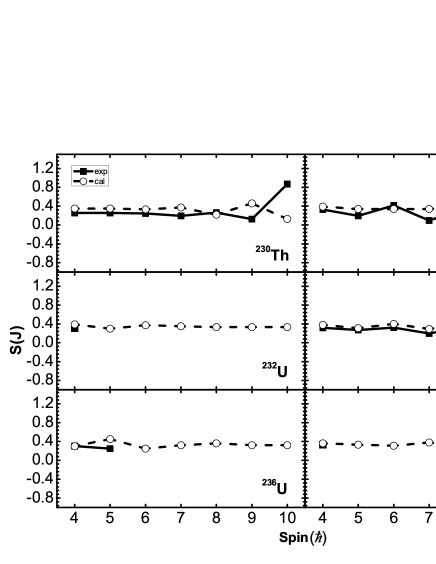
Figure 8: Comparison of the calculated $S(J)$ values of $\gamma$-vibrational bands with experimental data for ^230,232Th, ^232,234,236U and ²⁴⁰Pu, respectively.

In Refs. Zam91 ; Stag07 , the benchmark

$$S(J)=\frac{\{E[J^{+}_{\gamma}]-E[(J-1)^{+}_{\gamma}]\}-\{E[(J-1)^{+}_{\gamma}]-E[(J-2)^{+}_{\gamma}]\}}{E[2^{+}_{g}]},$$ (15)

is defined to estimate the non-axiality and softness of the $\gamma$ deformation. In the equation above, $E[J_{\gamma}^{+}]$ is the energy level of $\gamma$-bands with spin $J$, and $E[2_{g}^{+}]$ is the energy of the first excited state of the ground band. In the case of axially symmetric rotor, $S(J)$ is equal to 0.333, and the staggering around this value indicates the non-axial effect. In the microscopic viewpoint, the staggering indicates the mixing of bases with different $K^{\pi}$s  LZP10 . In Fig. 8, we plot the $S(J)$ values of both the observed and calculated $\gamma$-bands as a function of spin for all the six nuclei we studied. For ²³⁰Th, the calculated $S(J)$ values have small deviations from experimental data except at $J^{\pi}$=9⁺ and 10⁺. For ²³⁴U, the observed and calculated $S(J)$ values are nearly the same, and moreover, the staggering is still small. According to our calculation, the $S(J)$’s for ²³²U and ²⁴⁰Pu nearly keep constant 0.333 at low spins, well reproducing one experimental data, respectively. The calculated $S(J)$’s nearly keep constant at low spins for ²³²Th. However, the staggering of experimental $S(J)$ data is obvious, indicating the non-axial shapes of ²³²Th, and it may explain why the HSM calculation does not well reproduce the experimental $\gamma$-band for this nucleus. Moreover, for ²³⁶U, the staggering of the calculated values is very small, which indicates a good axial shape.

IV Conclusion

In order to describe simultaneously the single-particle and low-lying collective excitations for heavy nuclei, the PSM is extended to the HSM by adding the collective degrees of freedom, namely the $D$-pairs excitations, into PSM intrinsic basis. The study about the structure of the $D$-pairs indicates the method to construct $D_{0}$- and $D_{2}$-pair is reasonable by the linear combination of all the 2-qp states with $K^{\pi}=0^{+}$ $(K^{\pi}=2^{+})$ in the PSM truncated space. In this way, the $D_{0}$- and $D_{2}$-pair do show collectivity.

Based on the collectivity of $D$-pairs, the energy levels and $B(E2)$ transitions for the g-band, 2-qp and 4-qp excitations, and collective $\beta$-bands and $\gamma$-bands are described simultaneously in HSM for deformed actinide nuclei ^230,232Th, ^232,234,236U and ²⁴⁰Pu, respectively. The calculation well reproduces the $g$-bands, $\beta$ and $\gamma$-bands and some quasiparticle bands compared with the observed values, although for ²³²Th, the deviations between the calculated and observed $\gamma$-bands is big due to the non-axial deformations. In addition, some low-lying quasiparticle bands are predicted, awaiting experimental confirmation. For all the nuclei studied, the calculated $B(E2)$ values in the g-bands from $2^{+}_{g}$ to $0^{+}_{g}$ and from $4^{+}_{g}$ to $2^{+}_{g}$ and the inter-band ones agree with the experimental values.

We demonstrate that the HSM can describe simultaneously low-lying collective and quasi-particle excitations in deformed nuclei by the collective 1-$D$-pairs. Meanwhile, the model space is still kept tractable for heavy nuclear systems. Furthermore, HSM can also study 2-phonon excitations by adding 2-$D$-pairs into the intrinsic basis of PSM, which will be our future work. Along this line, HSM will become a powerful multi-major-shell shell model, useful for both well-deformed nuclei and transitional ones.

References

- (1) K. Hara and Y. Sun, Int. J. Mod. Phys. E 4, 637 (1995).
- (2) C.-L. W, D.-H. Feng, and M. Guidry, Adv. Nul. Phys 21, 227 (1994).
- (3) Y. Sun, X.-R. Zhou G.-L. Long, E.-G. Zhao, and P. M. Walker, Phys. Lett. B 589, 83 (2004).
- (4) F. Al-Khudair, G.-L. Long, and Y. Sun, Phys. Rev. C 79, 034320 (2009).
- (5) Y. Sun and M. Guidry, Phys. Rev. C 52, R2844 (1995).
- (6) Y. Sun, J.-y. Zhang, and M. Guidry, Phys. Rev. Lett. 78, 2321 (1997).
- (7) E. Caurier, J.-L. Egido, G. Martinez-Pinedo, A. Poves, J. Retamosa, L.-M. Robledo, and A.-P. Zuker, Phys. Rev. Lett. 75, 2466 (1995).
- (8) K. Hara, Y. Sun, and T. Mizusaki, Phys. Rev. Lett. 83, 1922 (1999).
- (9) G.-L. Long and Y. Sun, Phys. Rev. C 63, 021305 (2001).
- (10) J. A. Sheikh and K. Hara, Phys. Rev. Lett. 82, 3968 (1999).
- (11) J. A. Sheikh, G. H. Bhat, Y.-X. Liu F.-Q. Chen, and Y. Sun, Phys. Rev. C 84, 054314 (2011).
- (12) F. Iachello and A. Arima, The Interacting Boson Model (Combridge University Press, Cambridge, 1987).
- (13) F. Iachello, Phys. Rev. Lett. 53 1427-1429 (1984).
- (14) Y. Sun, C.-L. Wu, K. Bhatt, M. Guidry, and D.-H. Feng, Phys. Rev. Lett. 80, 672 (1998).
- (15) Y. Sun, C.-L. Wu, K. Bhatt, and M. Guidry, Nucl. Phys. A 703, 130-151 (2002).
- (16) Y. Sun and C.-L. Wu, Phys. Rev. C 68, 024315 (2003).
- (17) Y, Sun and C.-L. Wu, Int. J. Mod. Phys. E (suppl.) 17, 159 (2008).
- (18) J.-W. Cui, X.-R. Zhou, F.-Q. Chen, Y. Sun, and C.-L. Wu, Chin. Phys. Lett. 29, 022101 (2012).
- (19) Zhen-Hua Zhang, Jin-Yan Zeng, En-Guang Zhao, and Shan-Gui Zhou, Phys. Rev. C 83, 011304(R) (2011).
- (20) Zhen-Hua Zhang, Xiao-Tao He, Jin-Yan Zeng, En-Guang Zhao, and Shan-Gui Zhou, Phys. Rev. C 85, 014324(R) (2012).
- (21) J. Dudek, A. Majhofer, and J. Skalski, J. Phys. G: Nucl. Phys. 6, 447-454 (1980).
- (22) Z.-C. Gao, Y. Sun, and Y.-S. Chen, Phys. Rev. C 74, 054303 (2006).
- (23) Y.-S. Chen, Y. Sun, and Z.-C. Gao, Phys. Rev. C 77, 061305 (2008).
- (24) S. G. Nilsson et al., Nucl. Phys. A 131, 1 (1969).
- (25) T. Bengtsson and I. Ragnarsson, Nucl. Phys. A 436, 14 (1985).
- (26) J.-P. Delaroche, M. Girod, H. Goutte, and J. Libert, Nucl. Phys. A 771, 103-168 (2006).
- (27) H. Abusara, A. V. Afanasjev, and P. Ring, Phys. Rev. C 82, 044303 (2010).
- (28) D. R. Bs, P. Federman, E. Maqueda, and A. Zuker Nucl. Phys. 65, 1-20 (1965).
- (29) National Nuclear Data Center. http://www.nndc.bnl.gov/
- (30) Z.-P. Li, T. Niki, D. Vretenar, P. Ring, and J. Meng, Phys. Rev. C 81, 064321 (2010).
- (31) N. Pietralla and O. M. Gorbachenko, Phys. Rev. C 70, 011304(R) (2004).
- (32) R. F. Casten, Nuclear Structure from a Simple Perspective (Oxford University Press, 2000) p. 18-29.
- (33) N. V. Zamfir and R. F. Casten, Phys. Lett. B 260, 265 (1991).
- (34) E. A. McCutchan, D. Bonatsos, N. V. Zamfir, and R. F. Casten, Phys. Rev. C 76, 024306 (2007).