Dominance of most tolerant species in multi-type lattice Widom-Rowlinson models
Abstract
We analyse equilibrium phases in a multi-type lattice Widom–Rowlinson model with (i) four particle types, (ii) varying exclusion diameters between different particle types and (iii) large values of fugacity. Contrary to an expectation, it is not the most “aggressive” species, with largest diameters, which dominates the equilibrium measure, but the “most tolerant” one, which has smallest exclusion diameters. Results of numerical simulations are presented, showing densities of species in equilibrium phases and confirming the theoretical picture.
pacs:
05.20.-y, 02.50.Cw1 Introduction
The Widom–Rowlinson (WR) model was introduced in 1970 [1] as a simple continuum statistical physics model to study the thermodynamic equilibrium of a classical fluid in which one can rigorously analyse the existence of a liquid-vapor phase transition [2]. In its original formulation the WR-model is given in terms of a single type of particles in a continuum -dimensional space which have a specific interaction potential. It can be mapped onto a two-type mixture where particles of the same type do not interact and particles of different type interact according to a given pairwise hard-core exclusion diameter (ED) . Subsequently a lattice version of the model was introduced [3] as well as a generalisation for multiple types [4]. Aspects of these models have been studied e.g. in [3, 4, 5, 6, 7, 8, 9] (see also the bibliography therein). In the case of a multi-type model it was assumed that different particles have the same EDs. Recently [10] a variation of the multi-type continuum WR-model was introduced, with varying EDs between different particle types. Such models are interesting mathematically and may have applications in other fields including biology, medicine and sociology.
Biological examples of a multi-type WR-model are organism exhibiting allelopathy [11] such as certain algae, bacteria, coral, and fungi. A similar pattern is also related to growth of cancer cells lowering usual levels of tolerance [12, 13]. A natural question is which species will dominate after a long growth time when we reach an equilibrium measure, under a high rate of growth. A naïve guess might be that the most “aggressive” species, with largest EDs, will be predominant. But in fact, the equilibrium measure is dominated by a “most tolerant” species, with smallest EDs. A detailed understanding of this phenomenon is the main motivation of this work.
We analyze a lattice version of the -type WR-model in , for a large (and symmetric) fugacity , in analogy with a continuum model [10], adopting its notational system and terminology. Following [10], for we give a description of equilibrium measures in Proposition 1 (i) below. In addition, we analyze in detail the particle densities in these measures, cf. Proposition 1 (ii). Working in a lattice has an advantage of complementing theoretical results with numerical studies by using a suitable spin-flip process.
2 The -type lattice WR-model
We consider particles placed at nodes of a lattice , with the maximal occupancy number per site , i.e., at each site there is one or no particle. (There is a version of the model where the number of particles at a single node is unbounded; our theoretical results are extended to this case without major modifications.) In addition, each particle has an attached type ,…, , and no two particles of types , with can occupy sites with . Here stands for the graph distance in , and is a given collection of positive integers representing hard-core EDs.
An individual configuration is identified with a function . The configuration space of the model is denoted by ; formally,
| (3) |
Set and let denote a Bernoulli distribution where each site gets a label with probability and a label with probability where is a given number. Let denote a lattice cube: where is a positive integer. Given , define:
| (4) |
Here denotes the restriction of to , the restriction of to the complement and stands for the concatenation of the two restrictions. Then , and we consider the conditional distribution
| (5) |
In the literature, is called the Gibbs distribution in with a boundary condition . This distribution is associated to the grand canonical ensemble. When the configuration has , we write instead of .
We study DLR (Dobrushin-Lanford-Ruelle) measures [14, 15] supported by the event and satisfying the DLR equation (where is an unknown):
| (6) |
Here is a cube and a function depending upon the restriction . The DLR measures are obtained from the distributions via the thermodynamic limit, as .
In our approach we keep fixed the value and the collection (assumed to be of a general form) and let be close to . Thus, the fugacity is large. Moreover, as in [10], our results are given for ; for definiteness we focus on . A major issue are pure phases (PPs), i.e., shift-periodic ergodic DLR measures emerging as limits of distributions for dominant types . (The so-called staggering phases will not occur in our setting, cf. [9] and references therein.) It is well-known that for one has a unique DLR measure . This measure describes an infinite connected external cluster (a “sea”) of empty sites with (relatively rare) “islands” of occupied sites, inside which there may be “lakes” of empty sites containing smaller islands of occupied sites, etc. On the other hand, for both uniqueness and non-uniqueness of a PP can occur but the picture differs: the external cluster is occupied by a dominant particle type. A passage from one pattern to another, for a given pair but varying , is interpreted as a phase transition.
3 Dominant species in equilibrium phases
For , as in [10], we list the hard-core EDs in increasing order, omitting repetitions: . Here is the number of pair-wise distinct values among EDs . Define the vector with entries , :
| (7) |
giving the occupation numbers of the EDs for type . Take the collection of types for which the vector is lexicographically maximal (beginning with ):
| (8) |
Proposition 1
As in [10], assume the triangular condition
| (9) |
There exists a such that for all , we have the following properties:
(i) For , there exists the limiting measure
| (10) |
The measures are pairwise disjoint shift-invariant PPs. Any shift-periodic DLR measure is a mixture of , . In particular, for all , the distributions converge to a mixture of measures , with coefficients determined as in [10]. The measure has a unique infinite connected cluster of sites occupied by particles of type ; other species and empty sites produce finite clusters.
(ii) Given an and , a cube and a site , set . The following limits hold:
| (11) |
The value represents the type particle density in the measure whereas yields the “vacuum” density. The values satisfy a system of relations depending on the collection of the EDs . Viz., for , ,
| (12) |
As , monotonically with ,
| (13) |
A detailed mathematical proof of Proposition 1 will be given elsewhere. Instead, in the next section, we provide numerical evidence for the above proposition.
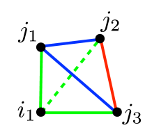
To understand this result, we visualise the particle types as vertices of a tetrahedron in ; cf. Figure 1. The edges are associated with . (We do not mean the length of an edge equals .) The number of distinct values for the EDs gives the number of different “colors” used for painting the edges. For instance, can be painted green, blue, red and so on.
In fact, homeomorphic colored pictures lead to equivalent models, with the same set of PPs. The total number of non-homeomorphic pictures equals : six-colored, five-colored, four-colored, three-colored, two-colored, single-colored.
The number of different PPs for a given is as follows.
-
1.
Four PPs occur in 4 pictures: 1 single-color, 2 two-color, 1 three-color (as in Figure 2 (a)).
-
2.
Three PPs occur in 1 two-color picture (as in Figure 2 (b)).
- 3.
-
4.
Finally, a single PP occurs in the remaining 267 pictures: 3 two-color, 25 three-color (see Figure 1 for an example), 59 four-color, 120 five-color, 60 six-color.
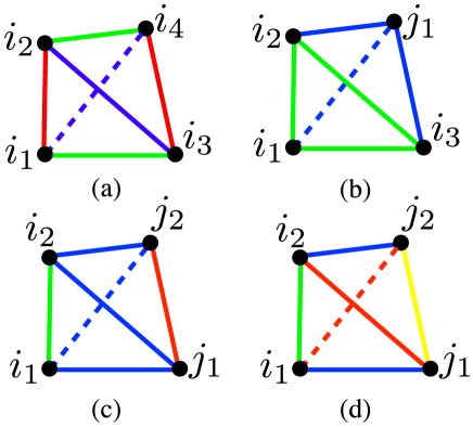
For example, in Figure 2(c) we have PPs for the dominant species . The types are more aggressive species.
The system of relations upon the densities , including (12), is established via symmetry considerations. For instance, in Figure 2(c), , and for we have the inequalities
| (14) |
4 A spin-flip process for simulating the lattice WR-model
Here we present numerical results obtained by using a discrete-time Markov spin-flip process. As was said, it can be interpreted as a physical process, describing the growth phenomenon behind the model.
The statistical weight under distribution is
| (15) |
where and represent the number of empty and occupied sites in . The transition probabilities are non-zero only when the configurations and differ at a single node . Dropping the index , we have the following transitions and their probabilities:
-
1.
If in is occupied: or ,
(16) (17) -
2.
If in is vacant: or ,
(18) (19)
Here denotes the configuration where all but one sites in preserve their status and site becomes vacant. Next, stands for the configuration where all sites in preserve their status except for which becomes occupied with a particle of type . Finally, gives the number of types for which .
Using (15)–(19), we get the detailed balance equation
| (20) |
This implies that the process iterations lead to distribution , close to the PP for a large .

Numerical simulations using the above spin-flip process were performed for species on a square in for various combinations of values of and collection . The number of iterations was . For a square the equilibrium is generally reached at iterations.
We have numerically verified the PPs for all examples shown in Figures 1 and 2, where we choose (green), (blue), (red), (yellow) and . When there are several PPs, we fix the boundary conditions accordingly. In all cases we obtained the correct PP.
As was said, for and a PP has a different structure. This points at a critical phenomenon at some . We record it numerically, with the relative frequency of the dominant species as a function of . This is done for the configuration of Figure 1 and Figure 2 (a)–(c) where we use the above values for EDs, square size and iterations. The result are shown in Figure 3. One observes the value for all cases after which the relative frequency of the dominant species becomes . It is interesting to observe that while all four examples show a phase transition just below , the configuration of Figure 2(a) provides evidence for an intermediate phase with a second transition at a lower value of . Note that in this case we have total symmetry between the four species and the result is qualitatively consistent with the case of equal EDs [8].

Another interesting aspect of the result of Proposition 1 is the relations between the densities of sub-dominant species. We analyse this numerically for the configuration of Figure 2 (c) where we record the densities for all four species for varying . The result is shown in Figure 4; it numerically verifies both the relations (12) and (13) and confirms the inequalities (14).
5 Discussion
We have introduced a multi-type lattice WR-model with varying hard-core exclusion diameters. We identify the pure phases (PPs) in the case of four species for all collections of hard-core EDs. Our analysis shows that the PPs are dominated by the “most tolerant” species, with smallest hard-core exclusion diameters (EDs). This is complemented with numerical results simulated using a spin-flip Markov process.
Regarding the analytical results we remark that it is in principle possible to go beyond four particle types or species. For , the particle types can again be placed at the vertices of a simplex in . As before, given a collection of hard-core EDs , we can list them in an increasing order and define the set of “lexicographically maximal” particle types. For , any dominant type belongs to . In particular, if , i.e., is reduced to a singleton, there is a unique DLR measure. Also, if coincides with the whole of , every type will be dominant. But in general not every type is dominant. An example is with five species and pair-wise distinct hard-core EDs, where . Here , and type is dominant but not; to determine this one needs to look at two-link paths along the edges of the five-vertex simplex (a pentagram).
As to the simulations, it is interesting to view the spin-flip process as a dynamical model, viz., of spread of cancer cells. Several lines in this direction are currently pursued.
Acknowledgements – The authors express their gratitude to Prof R. Chammas and Prof A. Ramos for providing references on cancer research and for numerous discussions on the applicability of the WR model in studies of tumor growth. This work is done under Grant 2011/51845-5 by FAPESP and Grant 2011.5.764.45.0 by USP. YS and IS thank IME, USP, for the hospitality. SZ was supported by FAPERJ (Grant 111.859/2012), CNPq (Grant 307700/2012-7) and PUC-Rio.
References
References
- [1] B. Widom, J. S. Rowlison, New model for the study of liquid-vapor phase transitions. J. Chem. Phys. 52 (1970) 1670.
- [2] D. Ruelle, Existence of a phase transition in a continuous classical system. Phys. Rev. Lett., 27 (1971), 1040.
- [3] J.L. Lebowitz, G. Gallavotti, Phase Transitions in Binary Lattice Systems. J. Math. Phys. 12 (1971), 1129
- [4] L.K. Runnels, J.L. Lebowitz, Phase transitions of a multicomponent Widom–Rowlinson model. J. Math. Phys. 15 (1974) 1712.
- [5] J.T. Chayes, L. Chayes, R. Kotecky. Comm. Math. Phys. 172 (1995), 449
- [6] J.L. Lebowitz, A. Mazel, P. Nielaba, L Samaj, Ordering and Demixing Transitions in Multicomponent Widom-Rowlinson Models. Phys. Rev. E 52 (1995) 5985.
- [7] R. Dickman, G. Stellb, Critical behavior of the Widom-Rowlinson lattice model. J. Chem. Phys., 102 (1995), 8674.
- [8] P. Nielaba, J.L. Lebowitz, (1997), Phase transitions in the multicomponent Widom-Rowlinson model and in hard cubes on the BCC-lattice. arXiv:cond-mat/976305.
- [9] H.-O. Georgii, V. Zagrebnov, Entropy-driven phase transitions in multitype lattice gas models. J. Stat. Phys., 102 (2001), 35.
- [10] A. Mazel, Y. Suhov, I. Stuhl, (2013), A classical WR model with particle types. submitted to Com. Math. Phys. arXiv:1311.0020.
- [11] E. L. Rice, Allelopathy, (1984), Academic Press.
- [12] L. Zhang, Y.-K. Lau, W. Xia, G.N. Hortobagy, M.C. Hung, Tyrosin kinase inhibitor emodin suppresses growth of HER-2/neu-overexpressing breast cancer cells in athymic mice and sensitizes these cells to the inhibitory effect of paclitaxel. Clin. Cancer Res. 5 (1999), 343.
- [13] J. Hickson et al. Societal interactions in ovarian cancer metastasis: a quorum-sensing hypothesis. Clin. Exp. Metastasis 26 (2009) 67.
- [14] R.L. Dobrushin. Description of a random field by means of conditional probabilities and the conditions governing its regularity. Theor. Prob. Appl. 13 (1968), 197.
- [15] O.E. Lanford, D. Ruelle. Observables at infinity and states with short range correlations in statistical mechanics. Comm. Math. Phys. 13 (1969), 194.