A Comparison of X-ray and Optical Emission in Cassiopeia A

Abstract

Broadband optical and narrowband Si XIII X-ray images of the young Galactic supernova remnant Cassiopeia A (Cas A) obtained over several decades are used to investigate spatial and temporal emission correlations on both large and small angular scales. The data examined consist of optical and near infrared ground-based and Hubble Space Telescope images taken between 1951 and 2011, and X-ray images from Einstein, ROSAT, and Chandra taken between 1979 and 2013. We find weak spatial correlations between the remnant’s X-ray and optical emission features on large scales, but several cases of good optical/X-ray correlations on small scales for features which have brightened due to recent interaction with the reverse shock. We also find instances where: (i) a time delay is observed between the appearance of a feature’s optical and X-ray emissions, (ii) displacements of several arcseconds between a feature’s X-ray and optical emission peaks and, (iii) regions showing no corresponding X-ray or optical emissions. To explain this behavior, we propose a highly inhomogeneous density model for Cas A’s ejecta consisting of small, dense optically emitting knots (n $\sim 10^{2-3}$ cm^-3) and a much lower density (n $\sim 0.1-1$ cm^-3) diffuse X-ray emitting component often spatially associated with optical emission knots. The X-ray emitting component is sometimes linked to optical clumps through shock induced mass ablation generating trailing material leading to spatially offset X-ray/optical emissions. A range of ejecta densities can also explain the observed X-ray/optical time delays since the remnant’s $\approx 5000$ km s^-1 reverse shock heats dense ejecta clumps to temperatures around $3\times 10^{4}$ K relatively quickly which then become optically bright while more diffuse ejecta become X-ray bright on longer timescales. Highly inhomogeneous ejecta as proposed here for Cas A may help explain some of the X-ray/optical emission features seen in other young core collapse SN remnants.

1. Introduction

With an estimated undecelerated explosion date around 1680 (Thorstensen et al., 2001; Fesen et al., 2006), Cassiopeia A (Cas A) is one of the youngest known Galactic supernova remnants (SNRs). It is also one of the few historic remnants with a secure supernova (SN) subtype through the detection of optical and infrared light echoes of its initial supernova outburst (Krause et al., 2008; Rest et al., 2008, 2011; Besel & Krause, 2012).

Optical spectra of its light echo show Cas A to be the remnant of a core-collapse Type IIb supernova event with an optical spectrum at maximum light similar to SN 1993J in M81. As indicated by the slow dense wind into which Cas A’s forward shock is expanding (Chevalier & Oishi, 2003; Hwang & Laming, 2009), the Cas A progenitor was probably a red supergiant with a mass of 15–25M_☉ that may have lost much of its hydrogen envelope to a binary interaction (Young et al., 2006; Hwang & Laming, 2012).

Viewed in X-rays, the remnant consists of a bright, line-emitting shell arising from reverse shocked ejecta rich in O, Si, S, Ar, Ca, and Fe (Fabian et al., 1980; Markert et al., 1983; Vink et al., 1996; Hughes et al., 2000; Willingale et al., 2002, 2003; Hwang & Laming, 2003; Laming & Hwang, 2003). Small knots and filamentary regions of X-ray emitting ejecta have been observed to change in intensity and structure over time, indicating the location of recently shocked, ionizing ejecta (Patnaude & Fesen, 2007). Exterior to this shell are faint X-ray filaments which mark the current location of the SNR’s $\simeq$ 5000 km s^-1 expanding forward shock (DeLaney et al., 2004; Patnaude & Fesen, 2009). This emission is largely nonthermal but can include faint line emission from shocked circumstellar material (CSM; Araya et al., 2010). This outer nonthermal X-ray emission is fading with time (Patnaude et al., 2011) while the bulk of the remnant’s bright thermal emission arising from shocked ejecta has remained relatively steady over the last few decades.

The remnant’s optical and infrared emissions trace the location of its denser debris ($\geqq 10^{3}$ cm^-3; Hurford & Fesen 1996; Fesen 2001) which in some places is co-spatial with lower density and more diffuse X-ray emitting material. The bulk of Cas A’s optical and near-infrared emission consists of a V_r = $-4000$ to $+6000$ km s^-1 expanding shell of knots, condensations, and filaments which lack any H$\alpha$ emission (Chevalier & Kirshner, 1978, 1979; Reed et al., 1995; DeLaney et al., 2010; Milisavljevic & Fesen, 2013). A few dozen semi-stationary condensations known as QSFs which do exhibit strong H$\alpha$ and [N II] $\lambda\lambda$6548, 6583 emissions with prevalently negative radial velocities of 0 to $-250$ km s^-1 appear to be pre-SN, circumstellar mass-loss material (van den Bergh & Dodd, 1970; van den Bergh, 1971; van den Bergh & Kamper, 1985; Reed et al., 1995).

In the picture of an inhomogeneous SN debris field with a range of ejecta densities and component dimensions, strong and widespread correlations between low density X-ray emitting material and small dense optically emitting knots are not expected; optical emission arises from gas with electron temperatures of around $\sim$ 30,000 K while X-rays arise from material shock heated to several million degrees K. Indeed, one generally sees only a weak spatial correlation of bright fine scale X-ray and optical features in images of Cas A taken at similar epochs (Laming & Hwang, 2003). But there are exceptions. For example, while noting only broad optical/X-ray emission coincidences in the remnant’s northern regions in the 1979 Einstein image, Fabian et al. (1980) cited an especially good correspondence between optical, X-ray, and radio emission in the bright optical Filament 1 of Baade & Minkowski (1954).

However, in places where dense optical emitting knots are embedded within or associated with a much lower density component there might be a close optical/X-ray emission correlation. The resemblance of the remnant’s morphology in the optical and Si and S X-ray emission lines is suggestive of at least some spatial coincidence (Hwang et al., 2000). Furthermore, indications of ejecta knot mass stripping in Cas A have been reported (Fesen et al., 2001, 2011) and such trailing material, if of the right density and mass, could lead to detectable associated X-ray emission downstream. Lastly, different excitation timescales between optical and X-ray emissions might lead to discernible time lags between the onset of strong optical and strong X-ray emissions.

Here we present the results of an investigation into X-ray and optical correlations that may be related to such factors through a comparative survey of Cas A’s optical and X-ray emission evolution over the last 30 years. The observations and results are described in $\S$2 and $\S$3, with a modeling analysis described in $\S$4. A summary of our findings and conclusions is given in $\S$5.

2. Observations and Data Reduction

2.1. X-Ray Imaging Data

The earliest X-ray images of Cas A with angular resolution capable of resolving features at scales $\sim$ 5$\arcsec$ were obtained in 1979 with the Einstein satellite and its High Resolution Imager (HRI). Details of the Einstein telescope and HRI detector can be found in Giacconi et al. (1979). The Einstein HRI has little spectral resolution over the 0.1–4.5 keV bandwidth of the telescope, and hence we used the broadband image without filtering any pulse height channels.

Cas A was not imaged again at high angular resolution until 1995–1996, with the ROSAT HRI, in the 0.2–2.4 keV band (Koralesky et al., 1998). Like the Einstein observations, we do not attempt any energy filtering of the ROSAT HRI data. Due to the high column density towards Cas A, the X-ray emission in this bandpass is dominated by thermal emission from Si XIII at $\simeq$ 1.85 keV.

More recently, Cas A has been extensively observed with the Chandra X-ray Observatory using the ACIS-S CCD detector. We summarize those observations (as well as the prior X-ray observations) used in this paper in Table 1. Since we are looking for correlations between Cas A’s X-ray and optical emissions and because a majority of archival optical images were particularly sensitive to [S II] $\lambda\lambda$6716,6731 emissions we focused our attention on the He-like ion emission of silicon in the Chandra X-ray data which should emphasize S + Si-rich ejecta.

We reprocessed all of the Chandra ACIS observations of Cas A using ciao 4.4.1 and CALDB 4.5.1 and then created exposure corrected images using the ciao script fluximage. Continuum image maps for the energy ranges 1.6–1.7 keV and 1.95–2.05 keV were generated, and we used them to estimate the continuum emission under the He–like silicon triplet. We then computed an exposure corrected image for Si XIII from 1.75–1.94 keV (centered on 1.85 keV) and subtracted the continuum emission image from that. This produces a map of emission that is mostly from Si XIII. We did this for each Chandra observation listed in Table 1.

The resulting Si XIII X-ray images were examined for time variable features in the form of the emergence or disappearance of individual knots and filaments. While there is evidence for variability in X-ray emission over short time scales (Patnaude & Fesen, 2007), here we investigated the time when certain X-ray knots first became visible in order to compare with the formation of coincident optical emission, where present.

For comparisons between Einstein, ROSAT, and Chandra observations we required a different strategy. Since we are unable to energy filter the Einstein and ROSAT observations, we chose to approximately match the Chandra observations to those HRI observations by energy filtering the ACIS-S data between 0.1–4.5 keV. However, the Chandra response below 0.3 keV is poorly characterized, so we only filter to 0.3 keV, and in any event low energy X-rays and XUV emission from Cas A are absorbed by a high column density (i.e., low energy X-rays from Cas A do not contribute much to the overall detected flux).

Several regions or features which showed significant flux variability using the 1979 Einstein image, the 1995 ROSAT image, and the calibrated 2000, 2004, 2007, 2010, and 2013 Chandra images (energy filtered between 0.3–4.5 keV) were identified and investigated. Using 5$\arcsec$ radius apertures, we extracted total counts from each data set for each region and compute the detector count rate, using the exposure times listed in Table 1. Hwang & Laming (2012) presented maps of the fitted X-ray temperature and absorbing column towards Cas A. For the purposes of this study, we assume that on average, the column towards Cas A is N_H $=$ 1.5$\times$10²² H atoms cm^-2, and $k_{\mathrm{B}}$T $=$ 1.8 keV. Using WebPIMMS, we converted the detector count rates into absorbed source fluxes, assuming a solar abundance APEC model with the above parameters. The results for five features discussed in § 3.2 are listed in Table 2. We note that while the APEC model does not accurately reflect the conditions we are investigating (it being a model for a plasma in collisional ionization equilibrium), we are using it to compute flux changes which give rise to the observed changes in count rate.

2.2. Optical Image Data

For optical observations of Cas A, we have made use of the extensive archival collection of Palomar Observatory 200 inch (5m) photographic plates taken of the remnant between 1951 and 1989 and made available though the assistance of S. van den Bergh. Added to this data set, are several more recent CCD images of Cas A taken with the MDM 1.3m and 2.4m telescopes obtained between 1992 and 1999 along with Hubble Space Telescope (HST) images of the remnant obtained from 2000 to 2011 (see Table 1).

2.2.1 Palomar Plates: 1951–1989

The majority of the optical imaging data are the Palomar 5m images, which comprise the earliest and deepest images taken of Cas A. These form a unique image set recording the remnant’s optical appearance soon after its 1948 discovery via radio observations (Ryle & Smith, 1948) and before the advent of high efficiency electronic detectors in the 1980s. These plates, $5\times$ 7 inches in size, were all taken at the Palomar 5m prime focus usually employing the Ross corrector plate and have a plate scale of $0.11\arcsec$ per mm. Filter and photographic emulsion details for each plate used or examined for this study are listed in Table 1.

These photographic plates, after being manually cleaned of surface dust, were digitized using the high-speed digitizing scanning machine DASCH (Simcoe et al., 2006; Laycock et al., 2010) at the Harvard–Smithsonian Center for Astrophysics. This scanner consists of a precision (0.2 $\mu$m) X-Y table, a red LED array, and a 4k $\times$ 4k CCD camera, and is capable of scanning two 8 $\times$ 10 inch plates in less than one minute. It can record the full dynamic range of the photographic negative (plate), and with its camera pixels just $11\mu$m in size is able to record plate details finer that the emulsion grains. Output is a set of overlapping frames which are then mosaiced together to form a single image of each frame. Approximate world coordinates (WCS) were determined for each plate using astrometric solutions done with an automated procedure using software routines in WCSTools (Laycock et al., 2010). More accurate WCS image coordinates were subsequently applied using USNO UCAC3 catalog stars (Zacharias et al., 2010) with a resulting estimated accuracy of $0\farcs 4$ near plate center.

2.2.2 Photometric Flux Measurements

Although the DASCH scanner is capable of generating accurate photometric data from photographic plates, we have not attempted to flux calibrate these images to the CCD images in our data set. This was viewed as an enormous undertaking (if even possible) and well beyond the scope and needs of this study. Aside from the lack of calibration plates taken from the same emulsion plate batches used for each of these images, the heterogeneous variety of photographic plate emulsions used over several decades (1951–1989), different chemical developers, development times and procedures means that the ‘characteristic curve’ of log(exposure) versus log(plate density) is likely to be different for every single plate (for further details see Laycock et al. 2010).

Apart from the photographic characteristic curve issue, calibrated optical magnitudes of the remnant’s emission line ejecta knots off the Palomar plates using a catalog of known magnitudes by assuming a non-linear function like that done for the similarly scanned Harvard College Observatory plate collection was also deemed not possible (Laycock et al., 2010). The Palomar plates taken of Cas A were obtained through a variety of uncalibrated broadband filters, and this taken together with the emission line nature of the remnant’s optical flux, i.e., unknown relative and possibly variable [O I], [O II], [S II], and [Ar III] emission line strengths within these filter passbands, greatly limits the meaning of the resulting photographic density to optical flux conversion.

The problem of measuring the equivalent of broad passband BVRI or Sloan filter optical magnitudes of Cas A’s emission knots even applies, although to a lesser extent, to modern CCD images. The remnant’s optical emission spectrum varies greatly across filaments and knots (Hurford & Fesen, 1996) and changes in the relative line strengths for individual ejecta knots have been observed, especially for ejecta rapid flux changes such as recently shocked ejecta knots (Morse et al., 2004; Fesen et al., 2011). Consequently, we have limited our optical/X-ray comparison survey only to those few coincident X-ray and optical emission knots or regions which exhibited obvious changes in flux.

Given these severe constraints, our estimated optical flux changes using the Palomar plates are limited only to gross changes in optical brightness for specific regions or features. Because magnitude values for late-type stars m_pg = 11.5 to 17.3) in the Cas A field made by van den Bergh (1971) were saturated on the Palomar plates we calibrated these images using USNO A2 red R2 magnitudes for a set of stars around the remnant in the magnitude range of 18.5 to 19.5. For red emulsion images using RG2, RG630, and RG645 filters, the internal consistency was a relatively modest $\pm 0.25$ mag given the uncalibrated plate material.

However, given the highly inhomogeneous optical image data, namely archival Palomar plate material, R band CCD images, and HST images taken with three different detectors and filter combinations (WFPC2 W675F, ACS F625W + F775W, and WFC3 F098M), we were unable to correlate optical fluxes of specific regions with meaningful accuracy. The basic problem is two-fold: 1) the different data sets employed different detectors having different wavelength sensitivities, and 2) a wide range of filters were used which either do not overlap each other, cover the same set of important emission lines, or have similar transmission at these line emission wavelengths. This situation made an accurate assessment of a feature’s optical flux changes not possible. Instead we present optical images of specific regions of interest where a qualitative assessment of a feature’s variability can be made in relation to other nearby remnant emission regions.

2.2.3 Blue vs. Red Images

For our comparison study of Cas A’s X-ray and optical emission structures, we chose to concentrate on red passband optical images. This decision was driven in part by the greater quality and quantity of Palomar red plates of Cas A (see Table 1) and the increased remnant’s structure when viewed at longer wavelengths due to more red line emissions than in the blue. Cas A’s blue optical line emissions are dominated by [O III] $\lambda\lambda$4959,5007 emission, whereas at longer wavelengths the remnant’s emissions arises from a larger number of strong emission lines including [O I] $\lambda\lambda$6300,6364, [S II] $\lambda\lambda$6716,6731, [Ar III]$\lambda$7135, and [O II]$\lambda\lambda$7319,7330.

As seen in Figure 1, while the remnant’s structure changes substantially between 1951 and 2004 and bright blue and red structures are consistent with one another, there are significant differences especially along the southern limb. Even in the northern regions where they are similar in gross morphology, remnant features are brighter and better detected in the red. Such differences are also due in part to the considerable interstellar reddening toward the remnant ($A_{V}$ = 4–6 mag; Hurford & Fesen 1996; Hwang & Laming 2012) which greatly weakens the remnant’s blue emission features. For these reasons, we focused most of our attention on the more complete data set of red optical images when comparing the remnant’s optical and X-ray emissions.

3. Results

Spatial correlations between Cas A’s optical and X-ray emission are generally not strong. Large scale emission correlations that do exist are mainly confined to the northern and northeastern regions (Laming & Hwang, 2003). This lack of strong correlation may be due in part to the relatively high and varied extinction along the line of sight to Cas A, especially along its western limb (Eriksen et al., 2009; Hwang & Laming, 2012). We have attempted to mitigate some of the effects of this absorption by using red and near infrared images sensitive to the remnant’s strong [S II] $\lambda\lambda$6716, 6731 and [S III] $\lambda\lambda$9069, 9531 line emissions and by examining the remnant’s X-ray emission from Si XIII at $\sim$ 1.8 keV which is not strongly affected by interstellar absorption.

In addition, by focusing on emission from silicon (in X-rays) and sulfur (in optical), one is sampling ejecta with like abundances, as these two elements are both synthesized during explosive oxygen burning. Using sulfur as a proxy for silicon is confirmed in the equivalent width maps of Cas A presented in Hwang et al. (2000). Using these X-ray and optical data sets, we discuss below our findings regarding large and small scale optical/X-ray comparisons, possible time delays between the appearance of optical and X-ray emissions, and selected regions that show no corresponding optical or X-ray emission.

3.1. Large Scale X-ray and Optical Emission Comparisons

From the first high-resolution X-ray image of Cas A taken with the Einstein satellite in 1979, it was clear that Cas A’s X-ray and optical morphologies exhibited significant large scale differences. This can be seen in Figure 2, where we contrast the remnant’s X-ray and optical emissions in the late 1970s and some 25 years later in 2004.

In the upper two panels of Figure 2, we show the 1979 Einstein HRI broadband image of Cas A along side of a deep 1976 Palomar Hale 5m red optical image. While there is some correlation between certain emission regions seen in the 1976 optical and 1979 X-ray images especially along the remnant’s northern limb, there is a poor large-scale optical/X-ray emission correlation over much of the remnant, especially notable in the remnant’s south, east, and west quadrants. Most obvious is the lack of bright optical emission in the 1976 Palomar image coincident with the X-ray bright eastern and southeastern limbs, and the virtual absence of any optical emission along the remnant’s western limb, where moderately bright X-ray emission is present.

There is a better correlation between X-ray and optical emissions in 2004 Chandra and Hubble Space Telescope images. In the lower panels of Figure 2, we show a 2004 continuum subtracted Si XIII X-ray image of Cas A taken with Chandra ACIS-S on the left and a 2004 Hubble Space Telescope ACS image on the right where we have co-added the F625W and F775W filter images to simulate a broad passband band R filter image approximating the red 1976 Palomar image. While there is now optical emission along the remnant’s southwestern limb which matches the X-ray, there is still little optical emission in the southeast where the remnant’s X-ray emission is especially strong and extensive. These similarities and differences can be more readily visible in Figure 3 where we present a color composite of 2004 optical (red) and X-ray (green) emissions.

The southeastern region of Cas A has consistently shown especially poor X-ray/optical emission correspondence. In order to examine this region more closely, we show in Figure 4 an enlarged comparison of 2004 X-ray and optical emissions along the remnant’s southeastern limb (upper panels) along with a color composite of these X-ray (green) and optical (red) images shown in the lower panels. Features with coincident X-ray and optical emissions appear yellow. As can be seen from this figure, one finds only sparse spatial correlations between optical and X-ray emission features in this portion of the remnant. In fact, the brightest X-ray feature in this region, marked by the white boxed region and shown enlarged in the lower right panel of Fig. 4, lies substantially offset from bright neighboring optical features. In $\S$4 below we will discuss possible explanations for such anti-correlations.

It is important to note that unlike much of its X-ray emission, the remnant’s overall optical emission has shown substantial changes over the last few decades, becoming both brighter and more pervasive. This is illustrated in Figure 5 where we present X-ray and optical images of the remnant over time spans of 31 and 60 years, respectively. In the top row we show the 1979 Einstein image, the 1995 ROSAT image along with a November 2010 (listed here as 2011) Si XIII Chandra X-ray image of Cas A smoothed to match the angular resolution of the earlier images. In the 12 lower panels, we show optical red passband images of Cas A from 1951 to 2011. This figure shows that while Cas A’s overall X-ray emission has undergone only fairly minor large scale changes over the last three decades, its optical appearance has gone from one of faint and sparse emission structures, to a bright and extensive emission morphology in 60 years.

Although the optical observations shown in Figure 5 cover a time span that is roughly twice that of the X-ray images, it is apparent that the bulk of the remnant’s gross X-ray emission evolves on a slower timescale than its optical emission. That is to say, Cas A looks fairly similar in 2011 as its did in 1979 when viewed in X-rays, whereas the remnant’s optical appearance has changed substantially in many regions on timescales of a decade or less.

3.2. Small Scale X-ray/Optical Emission Correlations

At Chandra’s ACIS resolution, Laming & Hwang (2003) found a significant fraction of Cas A’s X-ray emission consists of knots or small-scale clumps. They noted that most of these clumpy X-ray features do not coincide with the remnant’s high-velocity optical ejecta knots and concluded that they represent only mildly over-dense regions rather than true, high density ejecta knots.

However, there are a number of small-scale features where optical and X-ray emissions do appear to positionally coincide, especially in cases of recently brightened optical and X-ray ejecta clumps. Below, we present and discuss a few of such cases where it appears that the remnant’s advancing reverse shock has resulted in correlated optical and X-ray changes and we explore both the spatial and temporal properties of such features.

Figure 6 shows the locations of five small-scale features which have exhibited significant brightening in both X-rays and in the optical within the last few decades. These features, marked as A–E on the 2004 Chandra image, appear to be either absent or weak on earlier Einstein or ROSAT images yet currently rank among the remnant’s brightest small-scale X-ray features. The X-ray flux evolution of these five regions are listed in Table 2, shown in Figures 7–11, and briefly discussed below.

Feature A: The upper row of panels in Figure 7 show 1979, 1995, 2000, and 2011 X-ray images of a region, marked by $10\arcsec$ diameter red circles in the remnant’s north-central regions which brightened in X-rays between 1995 and 2000 (see Table 2). Similar circles in the lower panels mark the coincident optical ejecta knot seen in images taken between 1976 and 2011. Whereas by 2000 this feature was one of Cas A’s brightest X-ray emission knots, the coincident optical emission is weak and unremarkable in its optical emission from 1992 up to 2011. While virtually absent in the Palomar image prior to 1972 and greatly complicated by the presence of a nearby and stationary QSF in the earliest images, the knot had an estimated R2 magnitude of 20.9 in 1976 but 20.1 and 19.4 in 1996 and 1999 respectively, in line with its brightening in X-rays.

Feature B: Considerable clumpy emission is seen in the 2004 Chandra image of the remnant’s north-central region (Fig. 6). Enlargements of four Chandra X-ray images taken between 2000 and 2013 centered on one of these emission knots labeled Feature B are shown in the upper panels of Figure 8, along with corresponding optical images covering the epochs 1999 to 2011. Like that seen for Feature A, this region exhibited a significant X-ray and optical brightening after 2004 and will be discussed further in $\S$3.3.1 below.

Feature C: Figure 9 shows a comparison of an X-ray and optical emission for the extended Feature ‘C’ located along the remnant’s northernmost rim. These images reveal a dramatic increase in X-ray brightness between 2000 and 2013 preceded by a sharp increase in coincident optical emission between 1992 and 1999. The feature’s X-ray emission was relatively weak in 2000 but by 2011 was one of Cas A’s brightest emission knots. However, unlike the two previous cases, its coincident optical emission is relatively bright although not ranking among the remnant’s brightest optical features. Also, the evolution of the X-ray emission in this feature appears to follow that seen in the optical but delayed by several years. For example, the feature’s X-ray emission was only apparent in 2000 whereas optically it became detectable by the late 1980s, showed marked increases in 1992 and 1999 mirrored later in the X-rays between 2004 and 2007.

Feature D: This southern limb X-ray emission clump, shown in Figure 10 consists of a small complex of knots which became bright in both X-rays and optically after 2000. By 2004, this feature was one of the brightest X-ray knot complexes along the remnant’s southern limb. The feature’s morphology is somewhat extended and showed significant changes between 2004 and 2007.

Feature E: Located along Cas A’s western limb, this feature exhibited a dramatic increase in optical flux after 1996. Its X-ray flux also increased after 2000, showing a second sharp increase in X-ray flux after 2010. There is some indication of a time delay of around three to five years between the onsets of optical and X-ray brightening. However, this is hard to confirm, because like Feature D, this is a complex of emission knots and clumps with similar but not exactly matching optical and X-ray morphologies.

The optical morphology possibly tying these five X-ray/optical co-spatial emission regions together is examined in Figure 12. As shown in these March 2004 HST images, all five small-scale regions (A through E) exhibit a structure consisting of many small bright knots plus considerable surrounding diffuse emission. A similar small-scale structure is also seen for the X-ray bright northeastern feature known as “Filament 1” (Baade & Minkowski, 1954) and noted by Fabian et al. (1980) as a case of especially good X-ray/optical co-spatial emission. The combination of both a highly inhomogeneous density structure and the recent passage of the remnant’s reverse shock may account for the co-spatial X-ray and optical emission correlations observed for these regions.

3.3. Optical and X-ray Positional and Temporal Offsets

In addition to co-spatial X-ray and optical emission, we also found positional and temporal offsets between Cas A’s X-ray and optical emission. Figure 13 shows an enlargement of the color X-ray and optical composite shown in Figure 3 but now covering just the north-central portion of the remnant. This region was selected because it contains several coincident small scale optical/X-ray knots. Two emission features of special interest are marked by white circles. Feature 1 is an example of a positional offset between associated clumpy X-ray and optical emissions, while Feature 2 is a case of relatively bright X-ray emission patch having no corresponding present optical emission but coincident with an optical feature visible decades prior but no longer easily detected.

3.3.1 X-ray/Optical Emission Offsets

We begin by presenting evidence for small-scale spatial offsets between a clump’s X-ray and optical emission. The small knot marked as Feature 1 is one such example. It consists of a small ($<5\arcsec$) optically bright knot similar to several other knots located to the north and northwest of it and seemingly forming a chain of optically bright knots each with some coincident or nearly coincident X-ray emission. As can be seen in this figure, the optical knot marked as Feature 1 exhibits some associated X-ray emission but which is offset slightly to the west.

This positional offset is examined in greater detail in Figure 14 where we show 2000 through 2010 X-ray and optical images along side of a color X-ray/optical composite. The knot’s optical and X-ray emission fluxes increase substantially over this period. At all four epochs between 2000 and 2010, the knot’s associated X-ray emission is not precisely coincident with the knot’s optical emission, instead offset by a few arcseconds to the west. This is much greater than possible alignment WCS errors between the optical and X-ray images.

A clue to the nature of such X-ray/optical emission offsets may come from the positional offset case seen in a line of apparently recently shocked ejecta located near the remnant’s south central region, shown in Figure 15. Comprising part of small arcs of filaments and referred to as the ‘parentheses’ by DeLaney et al. (2010) (see their Fig. 13). This emission arc lies on the facing (blueshifted) hemisphere of Cas A (Milisavljevic & Fesen, 2013) and has been interpreted as the walls of a reverse shocked ejecta cavity (Milisavljevic & Fesen, 2014).

The morphology of this filamentary arc suggests the remnant’s reverse shock has passed over a line of dense ejecta clumps, leading to Rayleigh-Taylor head-tail structures along with some trailing diffuse emission seen visible in the HST ACS 2004 and WFC3 2011 images. Associated X-ray emission can be seen offset and west (i.e., behind) the line of optical knots again by a few arc seconds ($\simeq 1\times 10^{17}$ cm). The positional offset behind this arc of filaments along with the trailing diffuse emission is present from 2000 through 2011 and suggests X-ray emission is enhanced in lower density regions associated with and derived from post-shocked higher density ejecta clumps. This interpretation is supported by spectroscopic data indicating substantial velocity shears ($\simeq 1000$ km s^-1; Fesen et al. 2001) in some parts of the remnant.

3.3.2 X-ray/Optical Emission Delays

Some compact X-ray emission features seen in the Chandra images have little or no coincident (Laming & Hwang, 2003). One example is Feature 2 marked in Figure 13. As shown in the mosaic of optical images covering the time span between 1972 and 1996 presented in Figure 16, a relatively faint patch of optical emission appeared in the early 1970s, brightened in the 1970s and early 1980s but then faded considerably, becoming barely detectable by the mid-1990s. Summing the flux in a $5^{\prime\prime}\times 5^{\prime\prime}$ aperture box centered on this feature, we estimate R2 magnitudes to be 23.3 in 1970, 21.1 in 1972, 20.1 in 1976, 19.5 in 1983, 21.7 in 1989, and 21.5 in 1992. Deep HST images taken in 2000 and later reveal very little in the way of optical emission in this region. In contrast, Chandra images of this region show a relatively bright patch of X-ray emission which has remained roughly constant in strength from 2000 through 2013. The nature of such X-ray bright but optically faint ejecta may be related to low density ejecta regions which initially give rise to some faint optical emission but relatively strong X-ray flux at late times.

A similar optical/X-ray emission evolution can be seen in the northern extent of a thin chain of emission knots roughly 10 arcsec northeast of Feature 2 (see Figs. 13 and 16). In 1972, the northern most knot of this chain appears fairly bright in 1972 and 1976 Palomar images but has faded considerably by the 1990s, so much so as to be barely detectable in 1992 and 1996 MDM images. Despite its optical fading, associated X-ray emission is relatively strong as can be seen in the lower right-hand panel of Figure 16 showing a color composite of 2000 Chandra and HST images.

Opposite cases can also be seen, where one sees strong optical emission but no associated X-ray emission. Extensive and ever brightening optical emission along the remnant’s northwestern limb first appearing in the early 1980s exhibits no obvious corresponding X-ray emission, even weakly. Yet this region exhibits one of the clearest views of the advancement of the remnant’s reverse shock (Morse et al., 2004). Figure 17 compares the region’s optical emission with that seen in the X-rays. Whereas the westernmost portion of the circled region shows both bright optical and X-ray emission, the eastern portion exactly where the remnant’s advancing reverse shock front can be easily identified, has no obvious X-ray counterpart. If this is a case of a delay of associated X-ray emission and not simply a density effect limiting the X-ray emission, then the X-ray/optical time lag must be greater than 20 years.

Finally, Figure 18 shows a case of an X-ray bright filament which slowly formed between 2000 and 2010 in the northeast near the base of the NE jet, exhibits only faint optical emission (marked in the figure as “Feature 3”). Optical emission in this location is extremely faint prior to 2000 and only weakly visible in deep HST WFC3 F098M images taken in 2011. Using the ciao tool specextract, we extracted X-ray spectra for this region and fit the He-like silicon line centroid and measured the 1.75–2.0 keV line+continuum flux. The results from this analysis are listed in Table 3. Over the 12 years for which the X-ray data were analyzed, the fitted line centroid increases by $\gtrsim$ 10 eV while the 1.75–2.00 keV flux increases by nearly a factor of 3. This may be an example of a “young” and low density region that shows only X-ray emission. The east and southeast regions of Cas A, which show extensive diffuse X-ray emission but little or no correlated optical emission (see Fig. 4) may be other examples. A lack of strong optical emission in these X-ray bright regions may also be related to hydrodynamical effects that can smooth out ejecta inhomogeneities (Wongwathanarat et al., 2013).

4. Discussion

From the comparisons presented in $\S$3, we have identified four cases of X-ray/optical correlations or anti-correlations: 1) good optical/X-ray spatial and temporal correlations for small scale features which appear to have recently brightened due to a recent interaction with the remnant’s reverse shock front, 2) features whose optical brightening precedes the onset of associated X-ray emission, 3) optical emission and X-ray emission peaks which appear spatially offset but present at the same time, and 4) regions showing no corresponding X-ray or optical emissions. Below we explore various physical situations that might give rise to these cases.

4.1. Physical Parameters

We begin our discussion of X-ray/optical correlations by first laying out the general physical parameters and timescales involved. We assume that the supernova ejecta can be modeled as a multiphase plasma with a diffuse component that contains much if not the bulk of the material and gives rise to the observed X-ray emission. Additionally, we assume there is a significant population of compact, dense ejecta “clumps” that are mainly responsible for the remnant’s observed optical emission. There are relevant timescales associated with each of these components and our aim is to describe a relation between them that is consistent with X-ray and optical properties described previously.

For ejecta that has not yet been shocked by the remnant’s reverse shock front, both the diffuse and clumpy components will be co-moving. We model the low density component by an expanding ejecta cloud with number density of $n_{\mathrm{ej}}$ $\sim$ 1.0 cm^-3 (Laming & Hwang, 2003). This number density of $\sim$ 1.0 cm^-3 has recently been confirmed observationally by low frequency radio absorption measurements where the authors measured a density of $\approx$ 4 cm^-3 (DeLaney et al., 2014).

Embedded within the low density ejecta may be small clumps with densities $n_{\mathrm{c}}$ $\sim$ 100–1000 cm^-3. In this situation, we assume that the two components are co-moving and in pressure equilibrium, otherwise the dense knots would experience mass ablation due to ram-pressure stripping as they travel through the diffuse component. Thus,

$$n_{\mathrm{ej}}k_{B}T_{\mathrm{ej}}=n_{\mathrm{c}}k_{B}T_{\mathrm{c}}\,,$$ (1)

where $k_{B}$ is Boltzmann’s constant and $T_{\mathrm{ej}}$ and $T_{\mathrm{c}}$ are the temperatures of the diffuse and clumped components. The temperature of the clumps are thus $\sim$ 10^-2 – 10^-3 $T_{\mathrm{ej}}$. The density of ejecta clumps embedded within a low density envelope may not instantaneously change between the diffuse and clumpy components. We will argue below that such low density material surrounding dense knots may be responsible for some population of correlated X-ray and optical structures identified in the images described in $\S$3.

Since the diffuse and clumped components are co-spatial and co-moving, they will interact with the SNR reverse shock at the same time. We assume a $\gamma$ = 5/3 gas meaning that radiative and cosmic-ray losses are dynamically unimportant. Main shell ejecta are expanding with a velocity of $u_{\mathrm{ej}}$ = 4000-6000 km s^-1 (Minkowski, 1959; van den Bergh, 1971; Lawrence et al., 1995; DeLaney et al., 2010; Milisavljevic & Fesen, 2013), and the diffuse ejecta downstream from the shock (e.g., the shocked ejecta) has a velocity (3/4)$u_{\mathrm{ej}}$.

While we assume that the density between the diffuse and clumped components varies relatively smoothly, we can define a density contrast between the clumps and the diffuse component to be $\chi$ $\equiv$ $n_{c}/n_{ej}$ (Klein et al., 1994). It is the same whether we consider the shocked or unshocked ejecta since the shock compression is the same in both the diffuse and clumped components. The $n_{c}$ specified here is the maximum number density in the clump, and any calculations will thus represent an upper or lower limit on the computed value.

In the shocked component of the ejecta, we take the ram pressure equilibrium between the shocked clumps and shocked ejecta as being

$$n_{\mathrm{ej,s}}u_{\mathrm{ej,s}}^{2}=n_{\mathrm{c,s}}u_{\mathrm{c,s}}^{2}\,,$$ (2)

where the “s” subscript denotes a shocked quantity. Given that the density contrast between the clump and the diffuse component is invariant and is $\chi$ $=$ 100–1000, and the velocity of the shocked diffuse component is three quarters that of the unshocked diffuse component ($\approx$ 3750 km s^-1), the velocity of the shock that is driven into the clump is then $u_{\mathrm{c,s}}=\chi^{-1/2}u_{\mathrm{ej,s}}$ $\approx$ 100 - 400 km s^-1. For simplicity, we assume that $u_{\mathrm{c,s}}$ = 250 km s^-1.

4.2. Emission Timescales

We are now in a position to compute relevant timescales associated with the rise in X-ray emission and those associated with the optical emission and subsequent clump destruction. Since unshocked clumps are comparatively cold and do not emit strongly in the optical, we will estimate their size based on the size of the shocked clumps observed with HST. Fesen et al. (2001) and Fesen et al. (2011) estimate a radius for optically emitting clumps to be $a_{0}$ $\sim$ 10^15-16 cm.

The clump crossing time, $t_{ic}$, is defined as the time it takes the shock in the diffuse component to cross the clump:

$$t_{ic}\equiv\frac{2a_{0}}{u_{\mathrm{ej,s}}}\,,$$ (3)

and the time for the clump to be crushed by the clump shock is the cloud crushing time:

$$t_{cc}\equiv\frac{\chi^{1/2}a_{0}}{u_{\mathrm{ej,s}}}\,.$$ (4)

The resulting crossing time is short, on order of one year. In contrast, given the size and density contrast of the clump and the velocity of the surrounding ejecta field, the cloud crushing time is estimated to be $t_{cc}$ = 5–30 yr. This is consistent with the timescale for knots to appear and subsequently disappear (van den Bergh & Kamper, 1985), and also appears consistent with the rise in emission from small scale features like those seen in Figures 7 through  11.

While the shock crossing timescale is independent of radiative processes, the cooling timescale for ejecta clumps is given by

$$t_{cool}\equiv\frac{3k_{B}T_{c,s}/2}{n_{c,s}\Lambda(T_{c,s})}\,,$$ (5)

where $\Lambda(T_{c,s})$ $\approx$ 10^-22 erg cm³ s^-1, and $T_{c,s}$ is the temperature of the shocked clump material, T_c,s $\approx$ 30,000 K. The cooling time is $\lesssim$ 20 yr, comparable to the timescale for the clump to be destroyed by hydrodynamical processes. However, the cooling time does not account for the hydrodynamical destruction and mixing of the clump into the diffuse component. For comparison, the cooling time for the X-ray emitting material can also be calculated– for a temperature $T_{ej,s}$ $\approx$ 1 keV, a density $\sim$ 1–10 cm^-3, and $\Lambda(T_{ej,s})$ $\approx$ 10^-20 erg cm³ s^-1 (Hamilton & Sarazin, 1984), the resulting cooling time is $\sim$ 10^4-5 yr. It has been shown that conduction can mitigate the effects of radiative cooling in crushed clouds (Orlando et al., 2005), but here we note that the heating timescale (via conduction) is very much longer than the cooling time:

$$\left(\frac{t_{cool}}{t_{cond}}\right)\simeq 10^{6}\frac{T^{2}_{c,s}}{n_{c,s}a_{0}}<1\,,$$ (6)

so the effects of thermal conduction are not considered.

While the clump is being crushed and eventually destroyed by a 100 – 400 km s^-1 shock driven into it, the associated diffuse component is being shock heated. Diffuse ejecta is initially cold and partially neutral, with free electrons initially supplied mostly by photoionization of the expanding unshocked ejecta field. For the diffuse ejecta component, the timescale for thermalization of the electrons and the timescale to ionize to Li–, He–, and H–like ionization states are considered. For the diffuse component, cooling is not important as neither Bremstrahlung emission from the electrons nor line emission from ions are efficient coolants at the temperatures we are interested in, as noted earlier.

Electron heating is determined by

$$\frac{\mathrm{d}T_{\mathrm{elec}}}{\mathrm{d}t}=\frac{T_{\mathrm{ion}}-T_{\mathrm{elec}}}{t_{\mathrm{eq}}}\,,$$ (7)

where the relaxation timescale $t_{\mathrm{eq}}$ $\propto$ $n_{\mathrm{ion}}^{-1}$$\times$T${}_{\mathrm{ion}}^{3/2}$. In fact, the electrons do not need to reach thermal equilibrium with the ions. Instead they only need to reach temperatures of $\sim$ 1 keV ($\approx$ 1.2$\times$ 10⁷ K) to emit at X-ray wavelengths and be detectable through the intervening interstellar column. The above equation is not easily integrated but can be solved numerically.

A second timescale relevant to the X-ray emission is the ionization timescale, $n_{e}t$. For X-ray line emission to be important, ionization timescales of $\log{(n_{e}t)}$ $\simeq$ 9–11 are required. The ionization timescale is time dependent and also depends on the electron temperature given by

$$\frac{1}{n_{e}}\frac{\mathrm{D}f(X^{i})}{\mathrm{D}t} = C(X^{i-1},T_{e})f(X^{i-1})+\alpha(X^{i},T_{e})f(X^{i+1})$$

$$-[C(X^{i},T_{e})+\alpha(X^{i-1},T_{e})]f(X^{i})\ .$$

$f(X^{i})$ is the fractional ionization state of element $X$ in state $i$, and $C(X^{i},T_{e})$ and $\alpha(X^{i},T_{e})$ are the ionization and recombination rates out of and into ion Xⁱ, respectively.

We used a one dimensional numerical hydrodynamics code to study the evolution of the electron temperature and ionization of the diffuse component of the ejecta. This code is based on the numerical code VH-1 developed by Blondin & Lufkin (1993) to which we have added a non-equilibrium ionization calculation and prescription for electron heating, similar to that described in Patnaude et al. (2009) although we do not consider cosmic-ray losses here.

Hwang & Laming (2012) recently completed a census of the X-ray emitting ejecta in Cas A, and we have used their results for our one-dimensional hydrodynamical model. We model Cas A’s diffuse ejecta as an $n$ = 10 power law in velocity ($\rho_{\mathrm{ej}}$ $\propto$ $u_{\mathrm{ej}}^{-10}$) expanding into an isotropic stellar wind ($\rho_{\mathrm{amb}}$ $\propto$ $r^{-2}$) and assume 3M_☉ of ejecta and an explosion energy of 2$\times$10⁵¹ erg. For the progenitor’s stellar wind, we assume $v_{\mathrm{wind}}$ = 10 km s^-1 and $\dot{\mathrm{M}}$ = 2$\times$10^-5 M_☉ yr^-1 (Chevalier & Oishi, 2003).

The exact choice of explosion and wind parameters affects the final ionization state and dynamics of the gas but we are mainly looking for a trend in how the optical emission from dense ejecta clumps relates to the X-ray emission from a co-moving diffuse component. Consequently, we are not too concerned with the exact details, only in whether the thermalization timescale for electrons and the ionization timescale to He-like states is similar to the clump destruction and radiative cooling timescales.

In Figure 19, we plot the ionization age and electron temperature of shocked ejecta behind the reverse shock as a function of when the ejecta was shocked. As seen in this plot, electrons quickly thermalize to X-ray emitting temperatures, while only after some $\sim$ 20 yr does the ionization parameter becomes large enough that emission lines from He–like ions become important. Thus, at least phenomenologically, significant X-ray emission at locations where optical emission first becomes bright is consistent with an ejecta structure where dense clumps of ejecta are embedded in a more diffuse medium.

In the above model, we make no assumptions about the elemental abundance in the ejecta, and use cosmic abundances. However, since Cas A’s ejecta are highly metal rich, each ionization will, in fact, lead to a higher electron density per unit time than in the cosmic abundance case. Additionally, since the electron heating is $\propto$ Z², the heating rate in a metal rich plasma will be greater and result in higher electron temperatures. Thus, the parameters shown in Figure 19 represent lower limits on the true values.

In the sections that follow below, we describe how the observed X-ray/optical emission phenomena presented in $\S$3 can fit within the basic framework described above.

4.3. Time Delays Between Optical and X-ray Emission

As discussed in §3.3.2, several recently shocked features exhibit apparent time delays between the rise of optical and X-ray emission (e.g., Features C and E). A particularly interesting example is that of Feature 2 in the northern portion of the remnant (Fig. 13). As shown in Figure 16, a faint patch of optical emission appeared around 1972, became more easily visible in 1976 and 1983 Palomar images but then gradually faded, becoming nearly undetectable in deep 1992 and 1996 images. At this location, 2000 and 2004 red passband HST reveal a half dozen small and very faint optical clumps, some showing some even fainter surrounding diffuse emission. In contrast, as shown in the lower right frame of Figure 16, one sees relatively strong X-ray emission at this location in the Chandra image starting in 2000 and in all subsequent images up to the present.

One can interpret such emission changes within the framework of a cluster of relatively low density ejecta clumps interacting with the reverse shock some 20–40 years ago. A shock is driven into a region of moderately dense ejecta giving rise to detectable but nonetheless relatively weak optical emission. At the same time, a larger region of lower density ejecta associated with these optical clumps is eventually heated to $\sim$ 10⁷ K and ionized to He– and H–like charge states. The timescale for this process is some 30 – 40 years, roughly similar to that seen for Feature 2, and envisioned in Figure 20. During that time, the optical clumps cool radiatively, also on a timescale of about 20 – 30 years, thus explaining the near disappearance optically by the late 1990s.

4.4. Positional Offsets Between Optical and X-ray Emission

There are numerous places in the remnant where this is a clear offset or separation between a feature’s optical and its X-ray emission. Figure 14 presents one such example. Another is shown in Figure 15 and it is this line of optical knots that may give us a clue to what is causing this particular morphology here and elsewhere.

Figure 15 shows a curved line of optical emission along with displaced associated X-ray emission. These optical knots lie on the facing hemisphere of the remnant (DeLaney et al., 2010; Milisavljevic & Fesen, 2013). We have drawn in the apparent direction of motion in which the reverse shock is traveling for the line of emission knots. The morphology of the line of optical emission knots would suggest that the reverse shock has recently passed over them but their associated X-ray emission lies to the right (west) and behind the optical emission and thus closer to the reverse shock’s current location than the line of optical emission knots.

We propose that such X-ray/optical offsets is, in some cases, generated by shock induced mass ablation from dense optically emitting ejecta knots. In Figure 21, we present a schematic of how this X-ray/optical offset morphology can be produced. In the first frame, the reverse shock and the ejecta are seen to be separate. In the second frame, the reverse shock encounters dense ejecta knots, which are shocked and become bright in optical emission. Some of the knot material is ablated by the reverse shock, and advects away from the knots, remaining closer to the reverse shock (third frame of Fig. 21). This material is of a lower density than in the knots and so is shock heated to higher temperatures where it can become visible in X-rays.

The separation between X-ray and optical emission in Figures 14 and 15 is $\approx$ 2.5$\arcsec$. This corresponds to an advection timescale of 10 years for the dense knots. It is likely that in these scenarios, the X-ray emission seen at the reverse shock is not directly associated with material from the knots that are observed at the same epoch– but possibly from knots that previously encountered and were ablated by the reverse shock. In any event, the low density component at the reverse shock can be “refreshed” by recently ablated material.

A similar set of mass ablation phenomena appears to occur in the NE “jet” of Cas A. Here, there is substantial evidence for high velocity ejecta bullets with space velocities between 8000 and 14,000 km s^-1 (Fesen et al., 2006). As they move away from the remnant’s expansion center, they are shock heated via their interaction with the surrounding circumstellar material. Some mass is stripped off these ejecta clumps due to Kelvin-Helmholtz instabilities along the sides of the bullets leading to faint optical emission trails seen in HST images (Fesen et al., 2011). This stripped material will be of lower density and consequently shock heated to high temperatures, and becoming X-ray bright (Hwang et al., 2004; Laming et al., 2006) while lagging behind the optically bright material. In both sets of cases, a positional offset occurs due to mass ablation of less dense material from the ejecta knots (bullets) which is then shock heated to higher X-ray emitting temperatures.

4.5. Regions with Coincident X-ray and Optical Emission

As described in $\S$3.2, certain regions are bright in both optical and X-ray emission. These cases may be instances where optical clumps are embedded within or associated with an extended, lower density medium like that seen in Figure 12. Both the dense and less dense regions are shocked at the same time. The optical emission becomes bright and as it advects away from the reverse shock, the lower density region becomes bright as well, in X-rays. This is shown schematically in Figure 20. What differentiates this scenario from that presented in the previous section may be that the maximum density of the optically emitting material is possibly lower than in the very dense knots, and the contrast between the dense and diffuse components is less (or the transition between dense and diffuse components more gradual). It could also occur if we are viewing shocked ejecta with significant mass ablation along our line of sight. We note that Figure 20 can qualitatively describe both regions that show coincident X-ray and optical emission, as well as regions that show a time delay between X-ray and optical emission, if the density contrasts and knot envelope structure are appropriately chosen.

4.6. Regions with Neither Temporal or Spatial Correlations

Just as some regions have coincident optical and X-ray emission, there are other regions in the Cas A remnant that exhibit emission only in either optical or X-ray bands. These regions do not seem to have obvious positional or temporal offsets which might be attributed to ablation of dense ejecta knots.

One such region lies in the remnant’s northwest limb (Fig. 17) where the advance of Cas A’s reverse shock front can be readily identified in optical emission (Morse et al., 2004). Between 1976 and 1992, the optical emission from this region has brightened substantially. This is in contrast to the X-ray emission (upper panels of Fig. 17), which show no clearly discernible change between 1979 and 2011. Morse et al. (2004) estimated preshock densities in this region of 25 – 2500 cm^-3. Ram pressure equilibrium thus requires that the velocity of this shocked high density component to be $\approx$ 20–200 km s^-1. With these densities, it is not surprising that there is no correlated X-ray/optical emission in this region especially since it has evolved into a nearly continuous filament of optical emission.

In contrast to the optically bright region in the northwest with no corresponding X-ray emission, a completely opposite situation exists in the northeast near the base of the remnant’s NE jet. Shown in Figure 18 is a region of brightening X-ray emission with no corresponding optical emission. Between 2000 and 2010, the filament has brightened substantially, with little or no corresponding optical emission seen. Using Chandra observations between 2000 and 2012, we modeled both the Si-K 1.75–2.0 keV line flux and line centroid, and found that the flux has increased by nearly a factor of 3 in 12 years, and the line centroid has increased by 10 eV over the same period, indicating an ionizing plasma (see Table 3).

While these two cases are quite different, the underlying cause of the differences may again be attributed to ejecta density. In the case of the X-ray emission in the northeast, lack of optical emission here could be due to the ejecta density being too low ($\lesssim$ 1 cm^-3) resulting in a high velocity of the shocked ejecta (probably several thousand kilometers per second) thus making the conditions not conducive to the formation of optically bright filaments. A similar situation may help explain the copious X-ray emission in the east and southeast (Fig. 4) where one sees hardly any coincident optical emission. Milisavljevic & Fesen (2013) noted the presence of plumes and rings of ejecta in Cas A. In the east/southeast, the plume of ejecta here might be of low density or at least any inhomogeneities might be smoothed out by hydrodynamical effects and thus optical emission from dense knots is not expected.

The northwest line of optical filaments shown in Figure 17 presents the exact opposite scenario as that seen in the southeast. In this region, it is likely that the reverse shock is currently interacting with a nearly continuous sheet of relatively high density material. The shocks driven into this sheet are not strong enough to produce X-ray emission but does result in a nearly continuous filament of optical emission.

4.7. A Clump + Envelope Model for Cas A’s Ejecta

A large fraction of Cas A’s ejecta likely exists as a low density, diffuse component with densities $\sim$ 1 cm^-3. We suggest that embedded within this low density, diffuse component are clumps of varying densities, many with surrounding lower density envelope-like structures. Dense knots with relatively thin envelopes (where the transition from the diffuse to clumped ejecta is akin to a step function) give rise to a head–tail like structure after reverse shock passage, resulting in the shocked optical knots appearing downstream of associated X-ray emission which is located closer to the shock; e.g., as in Region 1, shown in Figure 14 or in the “parentheses” seen in Figure 15, and idealized in the schematic seen in Figure 21.

There are also dense ejecta clumps that are surrounded by a much broader, yet lower density, envelope (see Fig. 12). In these cases, the optical knots and X-ray emitting envelope remain co-spatial, though there may be time delays as the optical emission brightens and fades, and then the X-ray emission subsequently brightens. Finally, there are regions where there is either only optical emission, and no X-ray emission, or visa versa (see Figs. 16 - 18). Which type of emission one observes will mainly dependent upon the region’s density.

Taken together, these various emission morphologies point to the ejecta being mostly diffuse in volume but containing small over-densities of several orders of magnitude. The exact structure of the transition region between the diffuse and clumped component is what determines the time and spatial scales over which correlated emission is observed.

This ejecta structure model can also explain discrepancies in estimated expansion ages for Cas  A derived from various emission band observations. The remnant’s optical expansion rate is $\approx$ $0.3$% yr^-1 (Fesen, 2001; Thorstensen et al., 2001), while its X-ray expansion rate has been calculated to be $0.2$% yr^-1 (Koralesky et al., 1998; Vink et al., 1998; DeLaney et al., 2004). The diffuse X-ray emission which gives rise to the lower expansion rate (and hence higher expansion age) is more strongly decelerated by the reverse shock (5000 km s^-1 undecelerated, to $\approx$ 3750 km s^-1 decelerated), while the optical knots are hardly decelerated, remaining essentially ballistic. The X-ray emitting material that is ablated off dense ejecta clumps (bullets) and exhibiting a spatial offset from the optical emitting material is expected to show a range of decelerations most similar to the diffuse component but not as strongly decelerated leading to space motions not dissimilar from that of the bullets.

4.8. X-ray/Optical Correlations in Other Young SNRs

Optical and X-ray emission correlations have been discussed in the context of other young supernova remnants. Comparing [O III] observations of SNR G292.0+1.8 to an existing Chandra observation, Ghavamian et al. (2005) found a good correlation between optical fast moving knots and more diffuse X-ray emission. Similar to our ejecta model, they postulated that the [O III] emission in G292.0+1.8 originated from radiative shocks driven into knots with densities $\sim$ 10³ cm^-3 while the X-ray emission arose from the more diffuse interclump gas with densities of only a few.

Like G292.0+1.8, similar correspondences are observed in the Small Magellanic Cloud SNR 1E 0102-7219. Gaetz et al. (2000) noted that there were some correlations between O-bright X-ray filaments and interior [O III] filaments observed with HST Planetary Camera F5202N, but noted that the HST observations may have missed some high velocity [O III] emission that was Doppler-shifted out of the filter bandpass. Finkelstein et al. (2006) compared HST ACS observations of 1E 0102-7219 and found that the optical emission and X-ray emission are not exactly coincident with each other. This is consistent with the ejecta model presented here and by Ghavamian et al. (2005) namely, optical emission is embedded or offset from X-ray emission due to density effects and the finite time required to shock heat the ejecta to X-ray emitting temperatures.

5. Conclusions

We have presented optical observations of Cassiopeia A dating back to 1951 and up through 2011 and compare these data to X-ray observations taken with Einstein, ROSAT, and Chandra in order to investigate spatial correlations between X-ray and optical emissions. Due to the large differences in postshock densities and temperatures, the prevailing view has been that there is little correlation between ejecta that emits in X-rays and that which emits optically. However, our study shows that this is not always true. Taking into account the dynamical evolution of shocked ejecta and the relevant X-ray and optical timescales involved in the radiative and hydrodynamical evolution of shocked ejecta, we do find X-ray/optical correlations in many regions of Cas A.

We have identified four cases of correlations and anti-correlations between X-ray and optical emission in the shocked ejecta in Cas A. These are: 1) X-ray and optical emission time delays of years or even several decades where the optical emission for a region or feature shows up prior to its associated X-ray emission, 2) spatial offsets typically of a few arcseconds ($\approx 10^{17}$) cm) between a feature’s optical and X-ray emission emission peaks, 3) regions showing significant optical emission but with no corresponding X-ray emission, and 4) strong X-ray emitting regions having little if any positional coincident optical emission.

To explain these correlations and anti-correlations, we propose a highly inhomogeneous density model for Cas A’s ejecta consisting of: 1) small dense knots which rapidly form optical emission following reverse shock front passage embedded in a more extended and more diffuse lower density component giving rise to associated X-ray emission but sometimes showing a significant time delay relative to the optical, 2) shock induced mass ablation off dense ejecta clumps thereby generating trailing low density and X-ray emitted material and hence positionally offset from the optical emitting knots, 3) smooth and relatively continuous high density ejecta filaments or shell walls that never reach X-ray emitting temperature, or conversely, large extended regions consisting mainly of low density ejecta, both of which lead to X-ray/optical emission anti-correlations.

A highly inhomogeneous ejecta model as proposed here for Cas A may also help explain some of the X-ray/optical emission features seen in other young core collapse SN remnants. However it remains to be determined what dynamical and radiative properties of the explosion mechanism sets the relative volumes of a remnant’s low and high density ejecta, how these components are distributed and arranged in the expanding debris cloud, or what are the limits to range of ejecta densities as a function of elemental abundances and expansion velocity (e.g. Kifonidis et al., 2003). Further studies into some of the properties of Cas A’s interior unshocked ejecta like those reported by Smith et al. (2009), Isensee et al. (2010), Grefenstette et al. (2014) and Milisavljevic & Fesen (2014) may give us valuable insights to these issues.

Table 1Summary Log of Observations Used for this Analysis

Instrument	Date	Obs. ID	Exposure Time	Energy/Wavelength	Observer/PI
X-Ray				$\cdots$
Einstein HRI	1979-02-08	713	42.5 ks	0.1–4.5 keV	Seward
ROSAT HRI	1995-12-23	US500444H	175 ks	0.2–2.0 keV	Keohane
CXO ACIS-S	2000-01-30	00114	50.0 ks	0.3–10 keV	Holt
CXO ACIS-S	2002-02-06	01952	50.0 ks	0.3–10 keV	Rudnick
CXO ACIS-S	2004-02-08	05196	50.0 ks	0.3–10 keV	Hwang
CXO ACIS-S	2007-12-05	09117	25.0 ks	0.3–10 keV	Patnaude
CXO ACIS-S	2007-12-08	09773	25.0 ks	0.3–10 keV	Patnaude
CXO ACIS-S	2009-11-02	10935	25.0 ks	0.3–10 keV	Patnaude
CXO ACIS-S	2009-11-03	12020	25.0 ks	0.3–10 keV	Patnaude
CXO ACIS-S	2010-10-31	10936	31.0 ks	0.3–10 keV	Patnaude
CXO ACIS-S	2010-11-02	13177	19.0 ks	0.3–10 keV	Patnaude
CXO ACIS-S	2012-05-15	14229	49.0 ks	0.3–10 keV	Patnaude
CXO ACIS-S	2013-05-20	14480	49.0 ks	0.3–10 keV	Patnaude
Optical
Palomar Hale 5m	1951-09-09	PH520B	1800 s	blue: 103aO+GG1	Baade
Palomar Hale 5m	1951-11-01	PH553B	7200 s	red: 103aE+RG2	Baade
Palomar Hale 5m	1951-11-03	PH563B	7200 s	red: 103aE+RG2	Baade
Palomar Hale 5m	1953-08-11	PH778B	1500 s	blue: 103aO+GG1	Baade
Palomar Hale 5m	1953-08-13	PH793B	6120 s	red: 103aE+RG2	Baade
Palomar Hale 5m	1954-11-25	PH232M	5400 s	blue: 103aJ+GG11	Minkowski
Palomar Hale 5m	1954-11-26	PH236M	7200 s	red: 103aE+OR1	Minkowski
Palomar Hale 5m	1954-12-23	PH1159B	1800 s	blue: 103aO+GG1	Baade
Palomar Hale 5m	1957-09-21	PH1732B	5400 s	red: 103aF+RG2	Baade
Palomar Hale 5m	1957-09-22	PH1736B	2100 s	blue: 103aO+GG1	Baade
Palomar Hale 5m	1958-08-11	PH3033S	5400 s	red: 103aF+RG2	Shane
Palomar Hale 5m	1965-08-30	PH4815	5400 s	red: 103aE+0R1	Miller
Palomar Hale 5m	1967-10-04	PH5107A	4200 s	red: 103aE+RG2	Arp
Palomar Hale 5m	1968-09-26	PH5254vB	5400 s	red: 103aF+RG2	van den Bergh
Palomar Hale 5m	1968-09-26	PH5255vB	1500 s	blue: 103aD+GG11	van den Bergh
Palomar Hale 5m	1970-09-01	PH5643vB	7200 s	blue: 103aJ+GG475	van den Bergh
Palomar Hale 5m	1970-09-03	PH5648vB	7200 s	blue: 103aJ+GG475	van den Bergh
Palomar Hale 5m	1970-09-04	PH5659vB	7200 s	red: 103aE+RG630	van den Bergh
Palomar Hale 5m	1971-08-29	PH5946	5400 s	red: 103aF+RG630	Arp
Palomar Hale 5m	1972-09-09	PH6236vB	7200 s	blue: IIIaJ+GG7	van den Bergh
Palomar Hale 5m	1972-09-10	PH6249vB	7200 s	red: 103aF+RG2	van den Bergh
Palomar Hale 5m	1973-07-31	PH6555vB	3600 s	red: 098-04+RG2	van den Bergh
Palomar Hale 5m	1973-08-01	PH6562vB	7200 s	blue: 103aJ+GG7	van den Bergh
Palomar Hale 5m	1973-08-04	PH6573vB	12000 s	098+[S II](FWHM=166 A)	van den Bergh
Palomar Hale 5m	1973-08-13	PH6891vB	4200 s	red: 098-04+RG2	van den Bergh
Palomar Hale 5m	1974-08-14	PH6902vB	7200 s	blue: IIIaJ+GG7	van den Bergh
Palomar Hale 5m	1974-08-15	PH6914vB	7200 s	blue: 127-02+GG7	van den Bergh
Palomar Hale 5m	1975-07-18	PH7077vB	6000 s	red: 098-02+RG645	van den Bergh
Palomar Hale 5m	1976-06-30	PH7231vB	7200 s	blue: 127-04+GG7	van den Bergh
Palomar Hale 5m	1976-07-02	PH7252vB	7200 s	red: 098-04+RG645	van den Bergh
Palomar Hale 5m	1977-10-07	PH7425vB	5400 s	blue: 124-01+GG7	van den Bergh
Palomar Hale 5m	1977-10-08	PH7433vB	4500 s	red: 098-04+RG2	van den Bergh
Palomar Hale 5m	1977-10-10	PH7445vB	7200 s	blue: 103aJ+GG7	van den Bergh
Palomar Hale 5m	1980-07-13	PH7766vB	6000 s	red: 098-04+RG645	van den Bergh
Palomar Hale 5m	1980-07-14	PH7771vB	7200 s	blue: IIIaJ+GG7	van den Bergh
Palomar Hale 5m	1983-07-12	PH8192vB	6000 s	red: 098+RG645	van den Bergh
Palomar Hale 5m	1983-07-13	PH8199vB	8700 s	blue: 124-01:GG7	van den Bergh
Palomar Hale 5m	1983-07-14	PH8201vB	10800 s	098+[S II](FWHM=166 A)	van den Bergh
Palomar Hale 5m	1989-09-28	PH8202vB	7200 s	red: 098-04+RG645	van den Bergh
Palomar Hale 5m	1989-09-28	PH8204vB	7200 s	098+[S II](FWHM=166 A)	van den Bergh
Palomar Hale 5m	1989-09-29	PH8206vB	7200 s	red: 098-04+RG645	van den Bergh
Palomar Hale 5m	1989-09-29	PH8207vB	7200 s	blue: 103aJ+GG7	van den Bergh
MDM 1.3m	1992-07-04	$\cdots$	1000 s	6600–6800 Å: broad [S II]	Fesen
MDM 2.4m	1998-09-18	$\cdots$	2400 s	5600–8800 Å: R band	Fesen
MDM 2.4m	1999-10-15	$\cdots$	2400 s	5600–8800 Å: R band	Thorstensen
HST WFPC2	2000-01-23	U59T0*	1000 s	6000–7500 Å: F675W	Fesen
HST WFPC2	2002-01-09	U6D10*	1000 s	6000–7500 Å: F675W	Fesen
HST ACS/WFC	2004-12-05	J8ZM0*	2400 s	5500–7100 Å: F625W	Fesen
HST ACS/WFC	2004-12-05	J8ZM0*	2000 s	6900–8600 Å: F775W	Fesen
HST WFPC2	2008-02-05	UA5K0*	2400 s	6000–7500 Å: F675W	Patnaude
HST WFPC2	2008-06-02	UA5K0*	2400 s	6000–7500 Å: F675W	Patnaude
HST WFC3/IR	2010-10-28	IBID*	22.1 ks	9000–10700 Å: F098M	Fesen
HST WFC3/IR	2011-11-18	IBQH*	22.1 ks	9000–10700 Å: F098M	Fesen

Table 2Estimated 0.1-4.5 keV Absorbed X-ray Fluxes: 1979–2013

Observatory	Feature A	Feature B	Feature C	Feature D	Feature E
Einstein HRI (1979)	7.3$\pm$0.8	0.0$\pm$0.3	11.0$\pm$1.2	5.6$\pm$0.6	14.0$\pm$1.7
ROSAT HRI (1995)	9.4$\pm$1.1	5.5$\pm$0.5	11.0$\pm$0.9	12.0$\pm$1.3	14.0$\pm$1.3
Chandra ACIS-S (2000)	23.6$\pm$3.1	11.0$\pm$1.0	31.7$\pm$3.8	19.0$\pm$1.8	32.2$\pm$3.6
Chandra ACIS-S (2004)	26.4$\pm$2.1	14.1$\pm$1.3	32.7$\pm$3.3	23.9$\pm$2.2	39.9$\pm$4.0
Chandra ACIS-S (2007)	28.9$\pm$3.1	16.8$\pm$1.5	43.9$\pm$4.5	28.9$\pm$2.7	42.1$\pm$3.8
Chandra ACIS-S (2013)	40.0$\pm$3.8	23.8$\pm$2.5	57.4$\pm$5.5	32.9$\pm$3.6	49.1$\pm$5.1

Table 3Si-K line centroid and 1.75 – 2.0 keV modeled flux for northeast filament at the base of the “jet”: 2000–2012

Epoch	Line Centroid	Modeled Flux
	keV	10-13 erg cm-2 s-1
2000	1.852$\pm$0.003	2.9
2004	1.858$\pm$0.003	4.0
2008	1.862$\pm$0.002	6.3
2012	1.863$\pm$0.002	8.7

Figure 1.— Comparisons of blue and red broadband optical images of Cas A. Top panels show Cas A’s optical appearance from 1951 to 2004 in blue light and mainly sensitive to [O III] $\lambda\lambda$4959,5007 emission. Images shown are the 1951 and 1977 Palomar 5m plates PH520B and PH7445, respectively, along with a December 2004 F475W ACS HST image. Lower panels show Cas A over this same period of time in broadband red images dominated by [S II] $\lambda\lambda$6716,6731, [O I] $\lambda\lambda$6300,6364 and [O II] $\lambda\lambda$7320,7330 line emissions. The 1951 and 1976 Hale 5m images are plates PH563B and PH7252vB while the HST image is a co-add of December 2004 ACS F625W and F775W images.

Figure 2.— Comparison of gross emission differences of Cas A as seen in X-rays and optical. Left hand panels show the 1979 Einstein X-ray image and a 2004 Chandra continuum subtracted Si XIII X-ray image. Right hand panels show broadband red optical images taken at similar epochs to the X-ray images. The optical images are sensitive to line emission from [S II] $\lambda\lambda$6716,6731, [O I] $\lambda\lambda$6300,6364 and [O II] $\lambda\lambda$7320,7330. The Palomar Hale 5m image is the July 1976 plate PH7252vB while the HST image is a co-add of March 2004 ACS F625W and F775W images.

Figure 3.— A color composite of 2004 images of Cas A. The optical image (red) is a March 2004 HST ACS WFC broadband red image (F625W+F775W) while the X-ray image is a 2004 Chandra continuum subtracted Si XIII image.

Figure 4.— Comparison of the southeastern region of Cas A in X-rays and optical. The upper panels show the same 2004 Chandra Si and HST F625W + F775W images as in Figure 3 but now enlarged and covering just the remnant’s southeastern region. The lower left panel show a color composite of these images (optical = red, X-ray = green). The white boxed region in the lower left panel marks where the X-ray and optical emission is brightest and shown enlarged in the lower right panel.

Figure 5.— Comparative emission changes of Cas A’s X-ray and red optical emission over 31 and 60 years, respectively.Upper Panels: Einstein, ROSAT, and Chandra ACIS-S images of Cas A showing an apparent increase of clumpy emission features from 1979 to 2011. The Chandra image has been smoothed by a 9 pixel Gaussian to approximate the resolutions of the Einstein and ROSAT images. Lower 4 rows: Cas A in optical broadband red emission images from 1951 to 2011. The 1951 – 1989 images are Palomar Hale 5m plates PH563B, PH3033S, PH5254vB, PH6249vB, PH7252vB, PH7766vB, PH8192vB, PH8206vB, the 1992 and 1998 images are MDM 1.3m and 2.4m images, while the 2004 and 2011 are HST ACS F625W + F775W and WFC3 F098M images (see Table 1 for details). Note the considerable brightening of the remnant’s optical emission along northern and southern limbs, most dramatically seen between the early 1950s and the 1970s, but continuing up to the present.

Figure 6.— The 2004 Chandra ACIS-S image of Cas A with five regions marked which showed significant brightening.

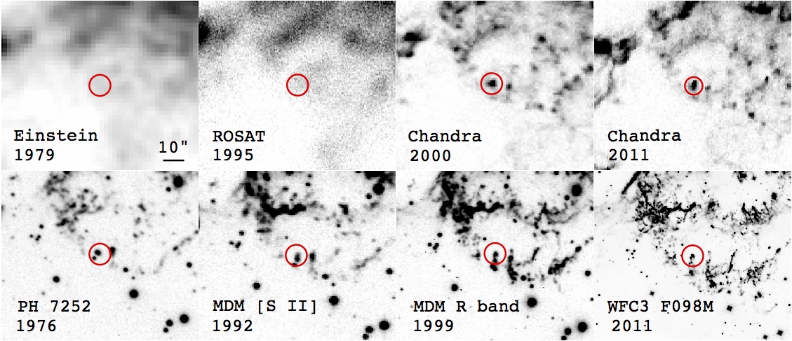
Figure 7.— Comparison of X-ray and optical emission for Feature ‘A’. Upper panels: Einstein, ROSAT and Chandra X-ray images with a circle 10$\arcsec$ in diameter centered on the Feature A’s approximate location. Lower panels: Images of coincident optical emission for this feature. Note: The circles are centered on the emission feature and follow the feature’s proper motion. In the 1976 and 1992 images, the optical knot is seen to cross in front of or behind a brighter stationary QSF emission knot.

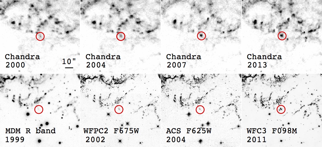
Figure 8.— Comparison of X-ray and optical emission for Feature ‘B’. Upper panels: 2000 to 2013 Chandra X-ray images of Feature B. The red circles (dia. = 10$\arcsec$) are centered on Feature ‘B’. Lower panels: Optical images of the area around Feature ’B’ at the same scale as the X-ray images. The ejecta knot responsible for the X-ray emtting Feature ‘B’ brightened considerably between 1999 and $2002$ in the optical and between 2000 and $2004$ in X-rays. The optical image sections shown are approximately centered on the emission feature but do not follow the feature’s proper motion.

Figure 9.— Comparison of X-ray and optical emission for Feature ‘C’. Upper panels: X-ray images of emission Feature C. The red circles have a diameter of 10$\arcsec$ on the X-ray images. Lower panels: Optical images. The red circle shown here has a diameter of 10$\arcsec$. The optical images are: Palomar 5m images PH3033S, PH5107, PH6249vB, PH7252vB, PH8192vB, PH8206vB, an MDM 1.3m image taken using a broad [S II] interference filter, and an MDM 2.4m image taken with an R filter. The optical image sections shown are approximately centered on the emission feature and follow the feature’s proper motion northward. These images show a dramatic increase in X-ray brightness between 2000 and 2011 and a sharp increase in optical brightness between 1989 and 1992.

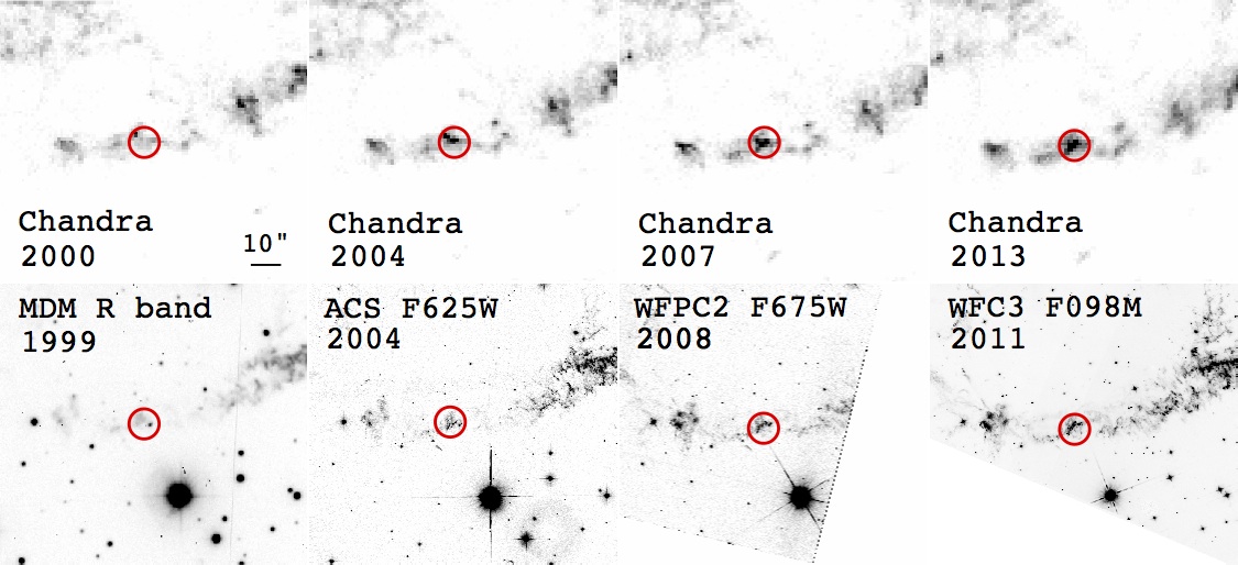
Figure 10.— Comparison of X-ray and optical emission for Feature ‘D’. Upper panels: X-ray images of emission Feature ’D’. The red circles have a diameter of 10$\arcsec$. Lower panels: Optical images of this feature. The images are: Palomar 5m images PH8202vB, a 1992 MDM 1.3m image taken using a broad [S II] interference filter, and an MDM 2.4m image taken with an R filter, and a 2008 HST WFPC2 F675W image. The optical image sections shown are approximately centered on the emission feature and follow the feature’s proper motion northward. These images show a steady increase in X-ray brightness between 2000 and 2011 and a sharp increase in optical brightness between 1992 and 1999.

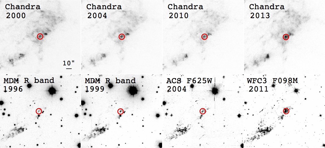
Figure 11.— Comparison of X-ray and optical emission for Feature ‘E’. Upper panels: X-ray images of emission Feature E. The red circles have a diameter of 10$\arcsec$ on the X-ray images. Lower Panels: Optical images of this feature. The images are a 1996 and 1999 MDM 2.4m R band image, a 2004 HST ACS F625W image, and a 2011 HST WFC F098M image. The optical images are approximately centered on the emission features and follow the feature’s proper motion approximately westward. These images show an increase in optical flux after 1996, and appeared in X-rays probably prior to 2000.

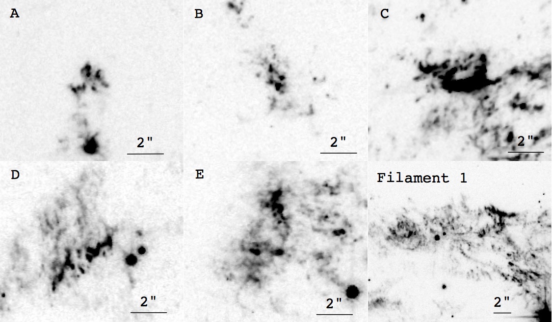
Figure 12.— Enlargements of the March 2004 ACS F625W+F775W merged image showing the detailed optical structures of Features A thru E plus the bright northeastern filament known as Baade and Minkowski’s Filament 1 which is one of the few good X-ray and optical spatial correlations. In all cases, numerous bright compact optical knots are seen embedded within or with considerable surrounding diffuse emission.

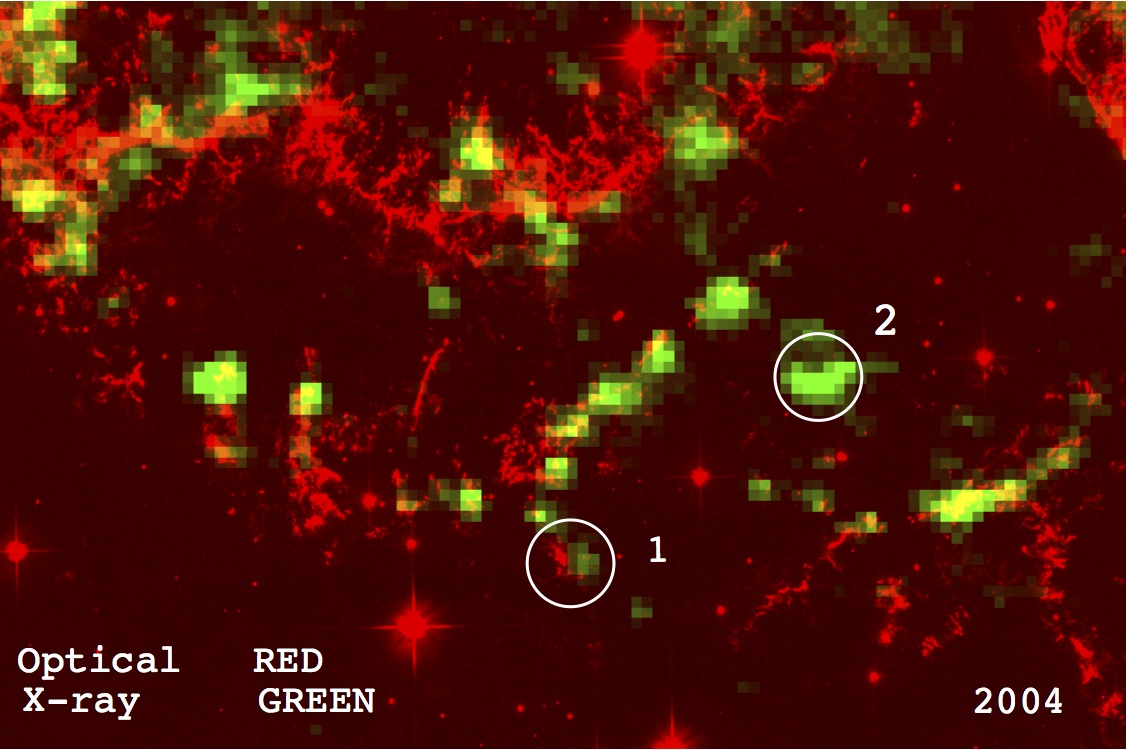
Figure 13.— Color composite of optical and X-ray images for the north-central region of Cas A showing several cases of positional correspondance of optical and X-ray features in 2004. Two small features are marked by white circles (dia. 8^′′) which are discussed in the text. Feature 1 is an example of a positional offset between optical and X-ray emission while Feature 2 marks an area with significant X-ray flux but lacking appreciable optical emission.

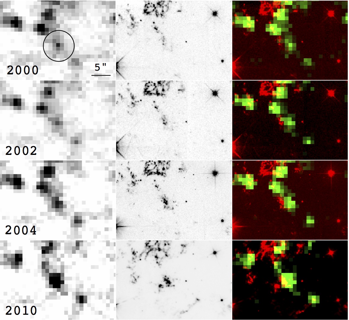
Figure 14.— A mosaic of 2000 – 2010 X-ray and optical images of a brightening ejecta knot (Feature 1; see Figure 13) are shown in Columns 1 and 2 respectively, with a color composite of these images shown in Column 3. The optical images are HST broadband red images while X-ray images (green) are Chandra continuum subtracted Si XIII image. North is up, East to the left. Note the positional offset to the west of the knot’s X-ray emission relative to its optical emission.

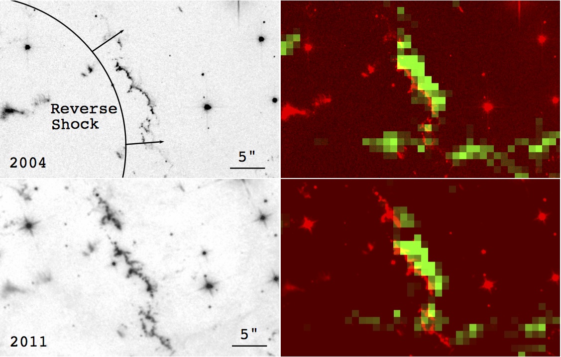
Figure 15.— A comparison of the March 2004 ACS F625W+F775W and the 2011 WFC3 F098M images and 2004 and 2011 Chandra Si XIII X-ray images of a line of ejecta filaments located southeast of the center of Cas A referred to as the ‘Parentheses’ by DeLaney et al. (2010). Note the positional offset on the X-ray emission behind the line of optical emission where there is apparent head-tail structure in these filaments, most visible in the 2011 [S III] HST WFC image. The line labeled reverse shock does not indicate the position of the reverse shock. The reverse shock lies to the northwest of the optical filaments, near the position of the X-ray emission.

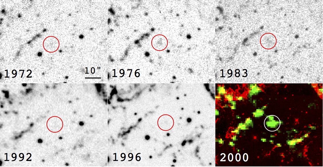
Figure 16.— A mosaic of optical images of Region 2 marked in Figure 13 covering the time span of 1972 to 1996 along with a color composite of a 2000 HST ACS WFC broadband red image (F625W+F775W) and a 2000 Chandra continuum subtracted Si XIII image. North is up, East to the left.

Figure 17.— Comparison of X-ray and optical emission for Cas A’s northwestern rim. The positions of the 30 arcsecond diameter red circles is the same on all X-ray and optical images. Upper panels: X-ray images of a region marked by a red circle where a substantial increase of optical filaments have appeared since the 1970s. Lower panels: A series of red optical images shows the development of a bright band of curved filaments between 1976 and 1999. The optical images shown are Palomar 5m images PH7252vB and PH8206vB, an MDM 1.3m image taken using a broad [S II] interference filter, and a MDM 2.4m image taken with an R filter. Since 1999 and through 2011, this band of bright optical filaments has remained bright and has become more extensive while in comparison only faint X-ray emission is seen in this region.

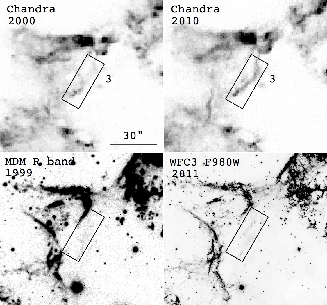
Figure 18.— X-ray and optical images of Cas A’s eastern limb showing the development of a bright X-ray filament with little associated optical emission.

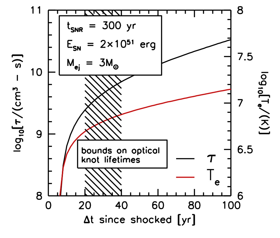
Figure 19.— Ionization parameter (black) and electron temperature (red) as a function of time since shocked. The model assumes an ejecta mass of 3M_☉, explosion energy of 2$\times$10⁵¹ erg, progenitor mass-loss rate of 2$\times$10^-5 M_☉ yr^-1 and a wind speed of 10 km s^-1. Also shown as a hatched region are the bounds on optical knot fading, either by radiative cooling or hydrodynamical destruction.

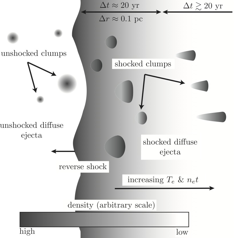
Figure 20.— Schematic representation of the structure of dense ejecta clumps. Dense clumps with density $n_{\mathrm{c}}$ embedded in a more diffuse component with density $n_{\mathrm{ej}}$ cross the reverse shock from left to right. The diffuse ejecta is decelerated to three quarters the unshocked velocity, and a slow shock is driven into the clumps. While a shock is driven into the clumps, they remain largely undecelerated by the reverse shock, due to their small cross section, and behave in a ballistic fashion until they are destroyed by hydrodynamical instabilities. At later times, the clumps have moved away from the reverse shock, and while they begin to fade, the diffuse component becomes bright in X-rays. These knots differ from those in Fig. 21 possibly due to the structure of the envelope which they are embedded in.

Figure 21.— Cartoon representation of dense knot ablation which leads to dense optical knots positioned downstream from X-ray emission, which appears closer to the reverse shock. In panel a, the unshocked knots are overtaken by the reverse shock. In panel b, a radiative shock is driven into the knots, and material is ablated off the sides of the knots, due to Kelvin–Helmholtz instabilities. In panel c, the ablated material appears as tails in optical emission, and as diffuse trailing emission in X-rays. Due to the lower velocity of the ablated material, it remains closer to the reverse shock position.

References

- Araya et al. (2010) Araya, M., Lomiashvili, D., Chang, C., Lyutikov, M., & Cui, W. 2010, ApJ, 714, 396
- Baade & Minkowski (1954) Baade, W., & Minkowski, R. 1954, ApJ, 119, 206
- Besel & Krause (2012) Besel, M.-A., & Krause, O. 2012, A&A, 541, L3
- Blondin & Lufkin (1993) Blondin, J. M., & Lufkin, E. A. 1993, ApJS, 88, 589
- Borkowski et al. (1989) Borkowski, K. J., Shull, J. M., & McKee, C. F. 1989, ApJ, 336, 979
- Chevalier & Kirshner (1978) Chevalier, R. A., & Kirshner, R. P. 1978, ApJ, 219, 931
- Chevalier & Kirshner (1979) Chevalier, R. A., & Kirshner, R. P. 1979, ApJ, 233, 154
- Chevalier & Oishi (2003) Chevalier, R. A., & Oishi, J. 2003, ApJ, 593, L23
- Claeys et al. (2011) Claeys, J. S. W., de Mink, S. E., Pols, O. R., Eldridge, J. J., & Baes, M. 2011, A&A, 528, A131
- DeLaney & Rudnick (2003) DeLaney, T., & Rudnick, L. 2003, ApJ, 589, 818
- DeLaney et al. (2004) DeLaney, T., Rudnick, L., Fesen, R. A., et al. 2004, ApJ, 613, 343
- DeLaney et al. (2010) DeLaney, T., et al. 2010, ApJ, 725, 2038
- DeLaney et al. (2014) DeLaney, T., Kassim, N. E., Rudnick, L., & Perley, R. A. 2014, arXiv:1403.0032
- Eriksen et al. (2009) Eriksen, K. A., Arnett, D., McCarthy, D. W., & Young, P. 2009, ApJ, 697, 29
- Fabian et al. (1980) Fabian, A. C., Willingale, R., Pye, J. P., Murray, S. S., & Fabbiano, G. 1980, MNRAS, 193, 175
- Fesen (2001) Fesen, R. A. 2001, ApJS, 133, 161
- Fesen et al. (2001) Fesen, R. A., Morse, J. A., Chevalier, R. A., et al. 2001, AJ, 122, 2644
- Fesen et al. (2006) Fesen, R. A., et al. 2006, ApJ, 645, 283
- Fesen et al. (2011) Fesen, R. A., Zastrow, J. A., Hammell, M. C., Shull, J. M., & Silvia, D. W. 2011, ApJ, 736, 109
- Finkelstein et al. (2006) Finkelstein, S. L., Morse, J. A., Green, J. C., et al. 2006, ApJ, 641, 919
- Gaetz et al. (2000) Gaetz, T. J., Butt, Y. M., Edgar, R. J., et al. 2000, ApJ, 534, L47
- Ghavamian et al. (2005) Ghavamian, P., Hughes, J. P., & Williams, T. B. 2005, ApJ, 635, 365
- Giacconi et al. (1979) Giacconi, R., Branduardi, G., Briel, U., et al. 1979, ApJ, 230, 540
- Grefenstette et al. (2014) Grefenstette, B. W., Harrison, F. A., Boggs, S. E., et al. 2014, Nature, 506, 339
- Hamilton & Sarazin (1984) Hamilton, A. J. S., & Sarazin, C. L. 1984, ApJ, 287, 282
- Hughes et al. (2000) Hughes, J. P., Rakowski, C. E., Burrows, D. N., & Slane, P. O. 2000, ApJ, 528, L109
- Hurford & Fesen (1996) Hurford, A. P., & Fesen, R. A. 1996, ApJ, 469, 246
- Hwang et al. (2000) Hwang, U., Holt, S. S., & Petre, R. 2000, ApJ, 537, L119
- Hwang & Laming (2003) Hwang, U., & Laming, J. M. 2003, ApJ, 597, 362
- Hwang et al. (2004) Hwang, U., Laming, J. M., Badenes, C., et al. 2004, ApJ, 615, L117
- Hwang & Laming (2009) Hwang, U., & Laming, J. M. 2009, ApJ, 703, 883
- Hwang & Laming (2012) Hwang, U., & Laming, J. M. 2012, ApJ, 746, 130
- Isensee et al. (2010) Isensee, K., Rudnick, L., DeLaney, T., et al. 2010, ApJ, 725, 2059
- Kifonidis et al. (2003) Kifonidis, K., Plewa, T., Janka, H.-T., & Müller, E. 2003, A&A, 408, 621
- Klein et al. (1994) Klein, R. I., McKee, C. F., & Colella, P. 1994, ApJ, 420, 213
- Koralesky et al. (1998) Koralesky, B., Rudnick, L., Gotthelf, E. V., & Keohane, J. W. 1998, ApJ, 505, L27
- Krause et al. (2008) Krause, O., Birkmann, S. M., Usuda, T., Hattori, T., Goto, M., Rieke, G. H., & Misselt, K. A. 2008, Science, 320, 1195
- Laming & Hwang (2003) Laming, J. M., & Hwang, U. 2003, ApJ, 597, 347
- Laming et al. (2006) Laming, J. M., Hwang, U., Radics, B., Lekli, G., & Takács, E. 2006, ApJ, 644, 260
- Lawrence et al. (1995) Lawrence, S. S., MacAlpine, G. M., Uomoto, A., et al. 1995, AJ, 109, 2635
- Laycock et al. (2010) Laycock, S., Tang, S., Grindlay, J., et al. 2010, AJ, 140, 1062
- Markert et al. (1983) Markert, T. H., Clark, G. W., Winkler, P. F., & Canizares, C. R. 1983, ApJ, 268, 134
- Masai (1994) Masai, K. 1994, ApJ, 437, 770
- Milisavljevic & Fesen (2013) Milisavljevic, D., & Fesen, R. A. 2013, ApJ, 772, 134
- Milisavljevic & Fesen (2014) Milisavljevic, D., & Fesen, R. A., 2013, in preparation
- Minkowski (1959) Minkowski, R. 1959, URSI Symp. 1: Paris Symposium on Radio Astronomy, 9, 315
- Morse et al. (2004) Morse, J. A., Fesen, R. A., Chevalier, R. A., et al. 2004, ApJ, 614, 727
- Orlando et al. (2005) Orlando, S., Peres, G., Reale, F., et al. 2005, A&A, 444, 505
- Patnaude & Fesen (2007) Patnaude, D. J., & Fesen, R. A. 2007, AJ, 133, 147
- Patnaude & Fesen (2009) Patnaude, D. J., & Fesen, R. A. 2009, ApJ, 697, 535
- Patnaude et al. (2009) Patnaude, D. J., Ellison, D. C., & Slane, P. 2009, ApJ, 696, 1956
- Patnaude et al. (2011) Patnaude, D. J., Vink, J., Laming, J. M., & Fesen, R. A. 2011, ApJ, 729, L28
- Reed et al. (1995) Reed, J. E., Hester, J. J., Fabian, A. C., & Winkler, P. F. 1995, ApJ, 440, 706
- Rest et al. (2008) Rest, A., et al. 2008, ApJ, 681, L81
- Rest et al. (2011) Rest, A., et al. 2011, ApJ, 732, 3
- Ryle & Smith (1948) Ryle, M., & Smith, F. G. 1948, Nature, 162, 462
- Schure et al. (2008) Schure, K. M., Vink, J., García-Segura, G., & Achterberg, A. 2008, ApJ, 686, 399
- Simcoe et al. (2006) Simcoe, R. J., Grindlay, J. E., Los, E. J., et al. 2006, Proc. SPIE, 6312,
- Smith et al. (2009) Smith, J. D. T., Rudnick, L., Delaney, T., Rho, J., Gomez, H., Kozasa, T., Reach, W., & Isensee, K. 2009, ApJ, 693, 713
- Sutherland & Dopita (1995) Sutherland, R. S., & Dopita, M. A. 1995, ApJ, 439, 381
- Thorstensen et al. (2001) Thorstensen, J. R., Fesen, R. A., & van den Bergh, S. 2001, AJ, 122, 297
- Truelove & McKee (1999) Truelove, J. K., & McKee, C. F. 1999, ApJS, 120, 299
- van den Bergh (1971) van den Bergh, S. 1971, ApJ, 165, 259
- van den Bergh (1971) van den Bergh, S. 1971, ApJ, 165, 457
- van den Bergh & Dodd (1970) van den Bergh, S., & Dodd, W. W. 1970, ApJ, 162, 485
- van den Bergh & Kamper (1985) van den Bergh, S., & Kamper, K. 1985, ApJ, 293, 537
- Vink et al. (1996) Vink, J., Kaastra, J. S., & Bleeker, J. A. M. 1996, A&A, 307, L41
- Vink et al. (1998) Vink, J., Bloemen, H., Kaastra, J. S., & Bleeker, J. A. M. 1998, A&A, 339, 201
- Willingale et al. (2002) Willingale, R., Bleeker, J. A. M., van der Heyden, K. J., Kaastra, J. S., & Vink, J. 2002, A&A, 381, 1039
- Willingale et al. (2003) Willingale, R., Bleeker, J. A. M., van der Heyden, K. J., & Kaastra, J. S. 2003, A&A, 398, 1021
- Wongwathanarat et al. (2013) Wongwathanarat, A., Janka, H.-T., Müller, E. 2013, A&A, 552, A126
- Young et al. (2006) Young, P. A., et al. 2006, ApJ, 640, 891
- Zacharias et al. (2010) Zacharias, N., Finch, C., Girard, T., et al. 2010, AJ, 139, 2184