Fuzzy transformations and extremality of Gibbs measures for the Potts model on a Cayley tree

Abstract.

We continue our study of the full set of translation-invariant splitting Gibbs measures (TISGMs, translation-invariant tree-indexed Markov chains) for the $q$-state Potts model on a Cayley tree. In our previous work [14] we gave a full description of the TISGMs, and showed in particular that at sufficiently low temperatures their number is $2^{q}-1$. In this paper we find some regions for the temperature parameter ensuring that a given TISGM is (non-)extreme in the set of all Gibbs measures. In particular we show the existence of a temperature interval for which there are at least $2^{q-1}+q$ extremal TISGMs. For the Cayley tree of order two we give explicit formulae and some numerical values.

Mathematics Subject Classifications (2010). 82B26 (primary); 60K35 (secondary)

Key words. Potts model, Critical temperature, Cayley tree, Gibbs measure, extreme measure, reconstruction problem.

1. Introduction

For the $q$-state Potts model on a Cayley tree of order $k\geq 2$ it has been known for a long time that at sufficiently low temperatures there are at least $q+1$ translation-invariant Gibbs measures which are also tree-indexed Markov chains [6], [7]. Such translation-invariant tree-indexed measures are equivalently called translation-invariant splitting Gibbs measures (TISGMs). One of the $q+1$ well-known measures mentioned above is obtained as the infinite-volume limit of finite dimensional Gibbs measures with free boundary conditions and each of the remaining $q$ measures is obtained as the limit with homogeneous (constant) spin-configurations as boundary conditions (see the next section for more details).

It is known (see, e.g., [8]) that for all $\beta>0$, the Gibbs measures form a non-empty convex compact set in the space of probability measures. Extreme measures, i.e. extreme points of this set are associated with pure phases. Furthermore, any Gibbs measure is an integral of extreme ones (the extreme decomposition).

The $q$ measures with homogeneous boundary conditions are always extremal in the set of all Gibbs-measures [6], [7], the free boundary condition measure is an extremal Gibbs measure only in an intermediate temperature interval below the transition temperature, and loses its extremality for even lower temperatures [24, Theorem 5.6.].

The non-trivial problem to determine the precise transition value is also equivalent to a reconstruction problem in information theoretic language. Indeed, the reconstruction problem is well-defined for any tree-indexed Markov chain defined in terms of a given transition matrix. The states we will consider are specific examples of such Markov chains. Single out a root vertex and denote by $\Pi^{a}_{n}$ the distribution of spins at distance $n$ from the root which is obtained by conditioning the spin at the root to be $a$. One says that the measure is reconstructable if there is a pair of symbols $a,b$ such that the total variational distance between $\Pi^{a}_{n}$ and $\Pi^{b}_{n}$ stays bounded against zero as the distance $n$ tends to infinity. In other words, some information about the symbol at the root survives a broadcasting even over arbitrary far distances, and this property is equivalent to non-triviality of the tail-sigma algebra, see [21]. It is well-known that non-triviality of the tail-sigma algebra is equivalent to non-extremality.

While the Kesten-Stigum bound gives a sufficient (but not necessary) bound in terms of the second largest eigenvalue of the transition matrix of the chain (and hence the temperature parameter) which ensures non-extremality [12],[25], the opposite problem, namely to ensure extremality in terms of bounds on parameters, is more difficult, and the known methods usually do not lead to sharp results for tree indexed Markov chains. This is true even in simple cases like the general asymmetric binary channel (or Ising model in a magnetic field). For the Potts model in zero field it was proved in [25] that the Kesten-Stigum bound for the free boundary condition measure is not sharp for $q\geq 5$. For some numerical investigations see [19].

For other results related to the Potts model and TISGMs on Cayley trees see [2], [9], [13], [14], [24] and the references therein.

Now, in [14] all TISGMs (tree-indexed Markov chains) for the Potts model are found on the Cayley tree of order $k\geq 2$, and it is shown that at sufficiently low temperatures their number is $2^{q}-1$. In the case $k=2$ the explicit formulae for the critical temperatures and all TISGMs are given.

The analysis was based on the classification of translation-invariant boundary laws which are in one-to-one correspondence with the TISGMs. The boundary laws are length-$q$ vectors with positive entries which satisfy a non-linear fixed-point equation (tree recursion), and a given boundary law defines the transition matrix of the corresponding Markov chain (see the next section for detailed definitions). It is an interesting but different issue to determine natural sets of boundary conditions of spin configurations for which the new states appear as finite volume limits. When chosen deterministically, such boundary conditions could be periodic but non-translation invariant, or they could be chosen from a natural measure to be constructed.

While the fact that these measures can never be nontrivial convex combinations of each other (i.e. extremal in the set of all TISGMs) is almost automatic (see [14, Theorem 2]) it is not clear whether and when they are extremal in the set of all Gibbs measures, including the non-translation invariant Gibbs measures.

In particular, from [14] it was not clear yet, whether the complete set of TISGMs contained any new extremal Gibbs measures beyond the known $q+1$ measures, or whether the new TIGSMs would all be non-extremal Gibbs measures. It is the purpose of this paper to give answers and find regions of parameters where a TISGM is (non-)extreme. To ask immediately for precise transition values, would be too much to ask for, in view of the known difficulty of the aforementioned reconstruction problem already for the free boundary condition measure.

The paper is organized as follows. Section 2 contains preliminaries (necessary definitions and facts). All of our analysis relies heavily on the following useful fact: While the full permutation symmetry of the free boundary condition measure is lost in general, all the $q\times q$ transition matrices which arise in the description of the TISGMs possess a $2\times 2$ block-structure. All possible sizes of blocks can appear, and labels within the blocks are equivalent. This corresponds to a decomposition of the $q$ spin-labels into two classes $1^{\prime}$ and $2^{\prime}$, one of $m$ elements, the other one of $q-m$ elements, with $m\leq q/2$. Such a structure invites the study of the associated fuzzy map (see [10], [13]) which identifies the spin-values within the classes, and which maps the Markov chain to a coarse-grained or fuzzy Markov chain with spin labels $1^{\prime},2^{\prime}$. It is interesting to note that this Markov chain can be interpreted as a splitting Gibbs measure for an effective Ising Hamiltonian with an external field, and that this Hamiltonian is independent of the choice of the Gibbs measure (within the class indexed by $m$). Such a result, namely the independence of the Hamiltonian for a transformed (renormalized) Gibbs measure of the phase, if this renormalized Hamiltonian exists at all, is known to be true for lattice models [3, 15] with proofs which are based on the Gibbs variational principle which holds for lattice systems but does not exist on trees.

Furthermore, [4] provides an explicit counterexample for such a theorem to hold in full generality, by showing that the Gibbs property of a time-evolved Ising tree measure does depend on the phase of the Ising model, in certain parameter regimes. It would be very interesting nevertheless to understand better to what extent the phenomenon of independence of the renormalized Hamiltonian of the phase for measures on trees we find here might generalize beyond the case we find in our example.

Section 3 is devoted to this fuzzy transformation of the Potts model to an Ising model with an external field. There we give a decomposition of the Potts measures in terms of their image measures under fuzzy transformation, and the conditional measure. We also study relations between eigenvalues of the relevant transition matrix given by the Potts model and by the corresponding fuzzy Potts model. We further derive conditions for extremality and non-extremality for the corresponding coarse-grained Markov chain.

We note that non-extremality of the coarse-grained chain already implies non-extremality of the original chain. Indeed, if the coarse-grained chain is not extremal then there is a tail-measurable event for the coarse-grained chain which has probability different from zero or one. But then the preimage of this event under the coarse-graining map is a tail-measurable event that has a probability different from zero or one under the original Potts measure, which therefore must also be not extremal.

Let us mention that sequences of coarse-graining maps to increasingly coarse spaces for which a temporal interpretation is natural have been considered in [11].

Section 4 is related to non-extremality conditions of a TISGM (for the original model), where we check the Kesten-Stigum condition (based on the second largest eigenvalue). We give explicit formulas for critical parameters for the Kesten-Stigum condition to hold. This provides us with sufficient conditions on the temperature to see non-extremality. We cannot expect these conditions to be sharp in general, since the Kesten-Stigum bound is not sharp in most cases, but often the Kesten-Stigum bound is numerically not very far off.

Section 5 deals with extremality conditions for a TISGM. There are various approaches in the literature to finding sufficient conditions for extremality which can be reduced to a finite-dimensional optimization problem based only on the transition matrix, see the percolation method of [18],[20], the symmetric entropy method of [5], or for the binary asymmetric channel (i.e., corresponding to an Ising model with an external field) the readily available bound of Martin [17]. Different techniques are used in [1] to show sharpness of the Kesten-Stigum bound for an Ising channel with very weak asymmetry.

In this paper we employ the approach of [18]. As in a particular temperature region there are many TISGMs which have different transition matrices which all lie in a sufficiently small neighborhood of the transition matrix of the free measure, and we know that extremality holds for the latter, a continuity (of parameters with respect to temperature) argument provides us with a lower bound on the number of extremal TISGMs which have to occur.

2. Preliminaries

Cayley tree. The Cayley tree $\Gamma^{k}$ of order $k\geq 1$ is an infinite tree, i.e., a connected graph without cycles, such that exactly $k+1$ edges originate from each vertex. Let $\Gamma^{k}=(V,L)$ where $V$ is the set of vertices and $L$ the set of edges. Two vertices $x$ and $y$ are called nearest neighbors if there exists an edge $l\in L$ connecting them. We will use the notation $l=\langle x,y\rangle$. A collection of distinct nearest neighbor pairs $\langle x,x_{1}\rangle,\langle x_{1},x_{2}\rangle,...,\langle x_{d-1},y\rangle$ is called a path from $x$ to $y$. The distance $d(x,y)$ on the Cayley tree is the number of edges of the shortest path from $x$ to $y$.

For a fixed $x^{0}\in V$, called the root, we set

$$W_{n}=\{x\in V\,|\,d(x,x^{0})=n\},\qquad V_{n}=\bigcup_{m=0}^{n}W_{m}$$

and denote

$$S(x)=\{y\in W_{n+1}:d(x,y)=1\},\ \ x\in W_{n},$$

the set of direct successors of $x$.

Potts model. We consider the Potts model on a Cayley tree, where to each vertex of the tree a spin variable is assigned which takes values in the local state space $\Phi:=\{1,2,\dots,q\}$. For $A\subseteq V$ a spin configuration $\sigma_{A}$ on $A$ is defined as a function

$$x\in A\to\sigma_{A}(x)\in\Phi.$$

The set of all configurations coincides with $\Omega_{A}=\Phi^{A}$. We denote $\Omega=\Omega_{V}$ and $\sigma=\sigma_{V}.$

The (formal) Hamiltonian of the Potts model is

$$H(\sigma)=-J\sum_{\langle x,y\rangle\in L}\delta_{\sigma(x)\sigma(y)},$$ (2.1)

where $J\in R$ is a coupling constant, $\langle x,y\rangle$ stands for nearest neighbor vertices and $\delta_{ij}$ is the Kroneker’s symbol:

$$\delta_{ij}=\left\{\begin{array}[]{ll}0,\ \ \mbox{if}\ \ i\neq j\\[5.69054pt] 1,\ \ \mbox{if}\ \ i=j.\end{array}\right.$$

In the present paper we only consider the case of ferromagnetic interaction $J>0$.

For a finite domain $D\subset V$ with the boundary condition $\varphi_{D^{c}}$ given on its complement $D^{c}=V\setminus D,$ the conditional Hamiltonian is

$$H(\sigma_{D}\big{|}\varphi_{D^{c}})=-J\sum_{{\langle x,y\rangle,\atop x,y\in D}}\delta_{\sigma(x)\sigma(y)}-J\sum_{{\langle x,y\rangle,\atop x\in D,\,y\in D^{c}}}\delta_{\sigma(x)\varphi(y)}.$$ (2.2)

Gibbs measure. A probability measure $\mu$ on $(\Omega,{\mathcal{B}})$ (where ${\mathcal{B}}$ is the $\sigma$-algebra generated by cylinder subsets of $\Omega$) is called a Gibbs measure (with Hamiltonian $H$) if it satisfies the Dobrushin-Lanford-Ruelle (DLR) equation: for all finite $D\subset V$ and $\sigma_{D}\in\Omega_{D}$:

$$\mu\left(\left\{\omega\in\Omega:\;\omega\big{|}_{D}=\sigma_{D}\right\}\right)=\int_{\Omega}\mu({\rm d}\varphi)\nu^{D}_{\varphi}(\sigma_{D}),$$ (2.3)

where $\nu^{D}_{\varphi}$ is the conditional probability (finite-volume Gibbs measure):

$$\nu^{D}_{\varphi}(\sigma_{D})=\frac{1}{Z_{D,\varphi}}\exp\;\left(-\beta H\left(\sigma_{D}\big{|}\,\varphi_{D^{c}}\right)\right).$$ (2.4)

Here $\beta={1\over T}$, where $T>0$ is the temperature and $Z_{D,\varphi}$ stands for the partition function in $D$, with the boundary condition $\varphi$:

$$Z_{D,\varphi}=\sum_{{\widetilde{\sigma}}_{D}\in\Omega_{D}}\exp\;\left(-\beta H\left({\widetilde{\sigma}}_{D}\,\big{|}\,\varphi_{D^{c}}\right)\right).$$

Splitting Gibbs measure. For $n\geq 1$ we denote by $\sigma_{n}$ a configuration $\sigma_{n}:V_{n}\to\Phi$, i.e., $\sigma_{n}\equiv\sigma_{V_{n}}=\{\sigma(x),x\in V_{n}\}$.

Define a distribution in the volume $V_{n}$ as

$$\mu_{n}(\sigma_{n})=Z_{n}^{-1}\exp\left\{-\beta H_{n}(\sigma_{n})+\sum_{x\in W_{n}}{\tilde{h}}_{\sigma(x),x}\right\},$$ (2.5)

where $Z_{n}^{-1}$ is the normalizing factor, $\{{\tilde{h}}_{x}=({\tilde{h}}_{1,x},\dots,{\tilde{h}}_{q,x})\in R^{q},x\in V\}$ is a collection of vectors and $H_{n}(\sigma_{n})$ is the restriction of the Hamiltonian to $V_{n}$, i.e.

$$H_{n}(\sigma_{n})=-J\sum_{\langle x,y\rangle\in V_{n}}\delta_{\sigma(x)\sigma(y)}.$$

We say that the probability distributions (2.5) are compatible if for all $n\geq 1$ and $\sigma_{n-1}\in\Phi^{V_{n-1}}$:

$$\sum_{\omega_{n}\in\Phi^{W_{n}}}\mu_{n}(\sigma_{n-1}\vee\omega_{n})=\mu_{n-1}(\sigma_{n-1}).$$ (2.6)

Here $\sigma_{n-1}\vee\omega_{n}$ is the concatenation of the configurations $\sigma_{n-1}$ and $\omega_{n}$. In this case, by Kolmogorov’s well-known extension theorem, there exists a unique measure $\mu$ on $\Phi^{V}$ such that, for all $n$ and $\sigma_{n}\in\Phi^{V_{n}}$,

$$\mu\left(\left\{\omega\in\Omega:\;\omega\big{|}_{V_{n}}=\sigma_{n}\right\}\right)=\mu_{n}(\sigma_{n}).$$ (2.7)

Such a measure is called a splitting Gibbs measure (SGM) corresponding to the Hamiltonian (2.1) and the vector-valued function ${\tilde{h}}_{x},x\in V$.

The following statement describes conditions on ${\tilde{h}}_{x}$ guaranteeing compatibility of $\mu_{n}(\sigma_{n})$.

Theorem 2.1.

(see [6], [24, p.106]) The probability distributions $\mu_{n}(\sigma_{n})$, $n=1,2,\ldots$, in (2.5) are compatible iff for any $x\in V\setminus\{x^{0}\}$ the following equation holds:

$$h_{x}=\sum_{y\in S(x)}F(h_{y},\theta),$$ (2.9)

where $F:h=(h_{1},\dots,h_{q-1})\in R^{q-1}\to F(h,\theta)=(F_{1},\dots,F_{q-1})\in R^{q-1}$ is defined as

$$F_{i}=\ln\left({(\theta-1)e^{h_{i}}+\sum_{j=1}^{q-1}e^{h_{j}}+1\over\theta+\sum_{j=1}^{q-1}e^{h_{j}}}\right),$$

$\theta=\exp(J\beta)$, $S(x)$ is the set of direct successors of $x$ and $h_{x}=\left(h_{1,x},\dots,h_{q-1,x}\right)$ with

$$h_{i,x}={\tilde{h}}_{i,x}-{\tilde{h}}_{q,x},\ \ i=1,\dots,q-1.$$ (2.10)

From Theorem 2.1 it follows that for any $h=\{h_{x},\ \ x\in V\}$ satisfying (2.9) there exists a unique SGM $\mu$ for the Potts model.

To compare with the literature we remark that the quantities $\exp(\tilde{h}_{i,x})$ define a boundary law in the sense of Definition 12.10 in Georgii’s book [8]. Here one should take the boundary law $z_{x,y}(i)=\exp(\tilde{h}_{i,x})$, where $y$ is the unique neighbor of $x$ that lies closer to $x^{0}$. Now all the other $z_{x,y}$ s can be calculated inductively from these using the definition of a boundary law, and this always yields a unique and well-defined boundary law.

The equation (2.9) can be written as the equation (12.15) in [8] for $z_{x,y}(i)$ normalized at $q$, i.e, assuming $z_{x,y}(q)\equiv 1$. Note that for a given $h_{x}=(h_{1,x},\dots,h_{q-1,x})$, assuming that $\tilde{h}_{q,x}$ is also some given number one can obtain $\tilde{h}_{i,x}$, $i=1,\dots,q-1$ from (2.10). Here the normalization of the boundary law mentioned above corresponds to the $\tilde{h}_{q,x}\equiv 0$. Thus by the normalization we reduce the $q$ dimensional vector to the $q-1$ dimensional vector. One can normalize the $q$ dimensional vector by the normalization at any other coordinate instead of $q$th coordinate. In this paper for definiteness we only consider the normalization at $q$.

Compare also Theorem 12.2 in [8] which describes the connection between boundary laws and finite-volume marginals of splitting Gibbs measures for general spin models. Formula (2.5) is a special case of this, since it was claimed only for volumes $V_{n}$ which were assumed to be balls on the graph. However, from the defining property of boundary laws as solutions to the fixed point equation it follows immediately that (2.5) extends to general subtrees $V_{n}$ of any shape, where $W_{n}$ is the inner boundary. For marginals on the two-site volumes which consist of two adjacent sites $x,y$, assuming a translation-invariant boundary law $z$ we have in the case of the Potts model

$$\mu(\sigma_{x}=i,\sigma_{y}=j)=\frac{1}{Z}z_{i}\exp(J\beta\delta_{ij})z_{j}.$$

From this the relation between the boundary law and the transition matrix for the associated tree-indexed Markov chain (splitting Gibbs measure) is immediately obtained from the formula of the conditional probability. Indeed, the corresponding transition matrix giving the probability to go from a state $i$ at site $x$ to a state to $j$ at the neighbor $y$ is then

$$P_{ij}={z_{j}\exp(J\beta\delta_{ij})\over\sum_{r=1}^{q}z_{r}\exp(J\beta\delta_{ir})}.$$ (2.11)

In the language of boundary fields: Once we have $\tilde{h}_{x}$ which is independent of $x$, i.e. $\tilde{h}=(\tilde{h}_{1},\dots,\tilde{h}_{q})$, then the tree-indexed Markov chain with states $\{1,2,\dots,q\}$ is given by the transition matrix $\mathbb{P}=(P_{ij})$ with

$$P_{ij}={\exp\left(J\beta\delta_{ij}+\tilde{h}_{j}\right)\over\sum_{r=1}^{q}\exp\left(J\beta\delta_{ir}+\tilde{h}_{r}\right)}.$$

Translation-invariant SGMs. A translation-invariant splitting Gibbs measure (TISGM) corresponds to a solution $h_{x}$ of (2.9) with $h_{x}=h=(h_{1},\dots,h_{q-1})\in R^{q-1}$ for all $x\in V$. Then from equation (2.9) we get $h=kF(h,\theta)$, and denoting $z_{i}=\exp(h_{i}),i=1,\dots,q-1$, the last equation can be written as

$$z_{i}=\left({(\theta-1)z_{i}+\sum_{j=1}^{q-1}z_{j}+1\over\theta+\sum_{j=1}^{q-1}z_{j}}\right)^{k},\ \ i=1,\dots,q-1.$$ (2.12)

In [14] all solutions of the equation (2.12) are given. By these solutions the full set of TISGMs is described. In particular, the following results are obtained which will be the starting point of the present analysis and which we repeat for convenience of the reader.

Theorem 2.2.

[14] For any solution $z=(z_{1},\dots,z_{q-1})$ of the system of equations (2.12) there exist $M\subset\{1,\dots,q-1\}$ and $z^{*}>0$ such that

$$z_{i}=\left\{\begin{array}[]{ll}1,\ \ \mbox{if}\ \ i\notin M\\[8.53581pt] z^{*},\ \ \mbox{if}\ \ i\in M.\end{array}\right.$$

Thus any TISGM of the Potts model corresponds to a solution of the following equation

$$z=f_{m}(z)\equiv\left({(\theta+m-1)z+q-m\over mz+q-m-1+\theta}\right)^{k},$$ (2.13)

for some $m=1,\dots,q-1$.

Remark 2.3.

We note that for each fixed $m$, the equation (2.13) has up to three solutions: $z_{0}=1,z_{i}=z_{i}(\theta,q,m),i=1,2$, with $z_{1}<z_{2}$ (see [14, Step 1 of the proof of Theorem 1]).

Denote

$$\theta_{m}=1+2\sqrt{m(q-m)},\ \ m=1,\dots,q-1.$$ (2.14)

It is easy to see that

$$\theta_{m}=\theta_{q-m}\ \ \mbox{and}\ \ \theta_{1}<\theta_{2}<\dots<\theta_{\lfloor{q\over 2}\rfloor-1}<\theta_{\lfloor{q\over 2}\rfloor}\leq q+1.$$ (2.15)

Proposition 2.4.

[14] Let $k=2$, $J>0$.

• If $\theta<\theta_{1}$ then there exists a unique TISGM;

• If $\theta_{m}<\theta<\theta_{m+1}$ for some $m=1,\dots,\lfloor{q\over 2}\rfloor-1$ then there are $1+2\sum_{s=1}^{m}{q\choose s}$ TISGMs which correspond (by Theorem 2.1) to the solutions $z_{r}\equiv z_{r}(\theta,q,s)=x^{2}_{r}(s,\theta)$, $r=1,2$, $s=1,\dots,m$ of (2.13), for $m=s$, i.e. $f_{s}(z)=z$, where

  $$\begin{array}[]{ll}x_{1}(s,\theta)={\theta-1-\sqrt{(\theta-1)^{2}-4s(q-s)}\over 2s},\\[5.69054pt] x_{2}(s,\theta)={\theta-1+\sqrt{(\theta-1)^{2}-4s(q-s)}\over 2s}.\end{array}$$ (2.16)

• If $\theta_{\lfloor{q\over 2}\rfloor}<\theta\neq q+1$ then there are $2^{q}-1$ TISGMs;

• If $\theta=q+1$ the number of TISGMs is as follows

  $$\left\{\begin{array}[]{ll}2^{q-1},\ \ \mbox{if}\ \ q\ \ \mbox{is odd}\\[5.69054pt] 2^{q-1}-{q-1\choose q/2},\ \ \mbox{if}\ \ q\ \ \mbox{is even;}\end{array}\right.$$

• If $\theta=\theta_{m}$, $m=1,\dots,\lfloor{q\over 2}\rfloor$,  ($\theta_{\lfloor{q\over 2}\rfloor}\neq q+1$) then number of TISGMs is

  $$1+{q\choose m}+2\sum_{s=1}^{m-1}{q\choose s}.$$

Remark 2.5.

We note that constants $\theta_{1}$, $\dots$, $\theta_{\lfloor{q\over 2}\rfloor}$ with similar properties as in Proposition 2.4 can be defined for general $k$, see [14, Theorem 1]. However, for $k\geq 3$ Theorem 1 of [14] gives only the existence of the corresponding solutions to the equation (2.13). To investigate the (non-)extremality for a given TISGM in this paper we need explicit formulas of these solutions, which we have only for $k=2$ by Proposition 2.4.

Remark 2.6.

For each fixed $m\leq\lfloor{q\over 2}\rfloor$, the symmetry of the Potts model allows us to reduce the study to at most three TISGMs: $\mu_{0}$ which corresponds to the solution $h_{x}=(0,\dots,0)$ and two TISGMs $\mu_{1}(\theta,m)$, $\mu_{2}(\theta,m)$ which correspond to the vectors

$$h_{x}=h_{1}=(\underbrace{\ln z_{1},\ln z_{1},\dots,\ln z_{1}}_{m},0,\dots,0),$$

$$h_{x}=h_{2}=(\underbrace{\ln z_{2},\ln z_{2},\dots,\ln z_{2}}_{m},0,\dots,0),$$

where $z_{1}=z_{1}(\theta,m)$ and $z_{2}=z_{2}(\theta,m)$ are solutions of the equation (2.13). Hence, for each given $m$ all TISGMs belong to three classes: the first class contains only $\mu_{0}$, the second class all measures which correspond to vectors obtained by permutations of coordinates of $h_{1}$, the last class contains all TISGMs which correspond to a vector obtained by permutations of $h_{2}$. It should also be noted that in case $m=q/2$ the solutions $h_{1}$ and $h_{2}$ define the same TISGMs after a relabeling of indices and a renormalization of $h_{1}$.

3. Fuzzy transformation to Ising model with an external field

In order to study extremality of a TISGM corresponding to a solution $z>0$, $z\neq 1$ of (2.13), (i.e. to a vector $l=(l_{1},\dots,l_{q})\in R^{q}$ with $m$ coordinates equal to $z$ and $q-m$ coordinates equal to 1) we divide the coordinates of this vector into two classes: We write $l^{\prime}$ and $l^{\prime\prime}$, where $l^{\prime}$ has $m$ coordinates each equal to $z$ and $l^{\prime\prime}$ has $q-m$ coordinates each equal to 1.

This is a particular case of the well-known fuzzy Potts model. The fuzzy Potts model on a given graph is obtained from a standard $q$-valued Potts model on the same graph by regrouping the possible spin-values into $r$ classes with $r<q$. The use of the word ’fuzzy’ suggests that only partial information of the underlying model is kept. To our knowledge this model has appeared for the first time as a lattice model in [16].

For our purposes we will not consider these general fuzzy transformations, but only transformations which are adapted to the symmetry of the Potts tree measures we have constructed. By this we mean that only those colors which behave similarly under the Potts tree measure will be put into the same class, as we will explain now.

Without loss of generality, by relabeling of coordinates, we can take $l$, $l^{\prime}$ and $l^{\prime\prime}$ as follows:

$$l=(\underbrace{z,z,\dots,z}_{m},\underbrace{1,1,\dots,1}_{q-m})=((\underbrace{z,z,\dots,z}_{m}),(\underbrace{1,1,\dots,1}_{q-m}))=(l^{\prime},l^{\prime\prime}).$$

Define a (fuzzy) map $T:\{1,2,\dots,q\}\to\{1^{\prime},2^{\prime}\}$ as

$$T(i)=\left\{\begin{array}[]{ll}1^{\prime},\ \ \mbox{if}\ \ i\leq m\\[5.69054pt] 2^{\prime},\ \ \mbox{if}\ \ i\geq m+1.\end{array}\right.$$ (3.1)

This map identifies spin-values which have the same value of the boundary law and are treated in an equal fashion by the transition matrix. We extend this map to act on infinite-volume spin configurations and measures in the infinite volume, i.e.

$$T(\sigma)(x)=T(\sigma(x)),\ \ T(\mu)(A)=\mu(T^{-1}(A)).$$

We note that a TISGM corresponding to a vector $l\in R^{q}$ is a tree-indexed Markov chain with states $\{1,2,\dots,q\}$ and transition probabilities matrix $\mathbb{P}=(P_{ij})$ with $P_{ij}$ given by (2.11).

From (2.11) we get

$$P_{ij}=\left\{\begin{array}[]{llllll}\theta z/Z_{1},\ \ \mbox{if}\ \ i=j,\,i\in\{1,\dots,m\}\\[5.69054pt] z/Z_{1},\ \ \mbox{if}\ \ i\neq j,\,i,j\in\{1,\dots,m\}\\[5.69054pt] 1/Z_{1},\ \ \mbox{if}\ \ i\in\{1,\dots,m\},j\in\{m+1,\dots,q\}\\[5.69054pt] z/Z_{2},\ \ \mbox{if}\ \ i\in\{m+1,\dots,q\},j\in\{1,\dots,m\}\\[5.69054pt] \theta/Z_{2},\ \ \mbox{if}\ \ i=j,\,i\in\{m+1,\dots,q\}\\[5.69054pt] 1/Z_{2},\ \ \mbox{if}\ \ i\neq j,\,i,j\in\{m+1,\dots,q\},\end{array}\right.$$ (3.2)

where

$$Z_{1}=(\theta+m-1)z+q-m,\ \ \ Z_{2}=mz+\theta+q-m-1.$$

The fuzzy map $T$ reduces the matrix $\mathbb{P}$ to the $2\times 2$ matrix $T(\mathbb{P})=\hat{\mathbb{P}}=(p_{ij})_{i,j=1^{\prime},2^{\prime}}$ with

$$p_{ij}=\left\{\begin{array}[]{llll}{(\theta+m-1)z\over Z_{1}},\ \ \mbox{if}\ \ i=j=1^{\prime}\\[5.69054pt] {q-m\over Z_{1}},\ \ \ \ \ \ \mbox{if}\ \ i=1^{\prime},j=2^{\prime}\\[5.69054pt] {mz\over Z_{2}},\ \ \ \ \ \ \mbox{if}\ \ i=2^{\prime},j=1^{\prime}\\[5.69054pt] {\theta+q-m-1\over Z_{2}},\ \ \mbox{if}\ \ i=j=2^{\prime}.\end{array}\right.$$ (3.3)

More precisely this means: Consider the translation-invariant tree-indexed Markov chain $\mu$ with transition matrix given by (3.2). Then its image measure $T(\mu)$ under the site-wise application of the fuzzy map $T$ is a tree-indexed Markov chain with local state space $1^{\prime},2^{\prime}$ with the transition matrix given by (3.3).

Note that an application to a Gibbs measure which is a Markov chain, of a transformation which is not adapted to the structure of the transition matrix (for example a fuzzy map which identifies spin values which have different values of the boundary law) would in general not give rise to a Markov chain (and possibly not even to a Gibbs measure with an absolutely summable interaction potential).

We also observe the following fact: If a Markov chain $\mu$ is extremal in the set of Gibbs-measures for the Potts model then this implies its triviality on the tail-sigma algebra of the $q$-spin events (see [8, Theorem 7.7]). Indeed, the extremality of Gibbs measures on any graph is equivalently characterized by the triviality of the measure on the tail-sigma algebra. But this implies that the mapped chain $T(\mu)$ is trivial on its tail-sigma algebra (since the latter can be identified with the sub-sigma algebra of events in the tail-sigma algebra of the $q$-spin events which do not distinguish spin-values which have the same values of the fuzzy variable).

It turns out that we can lift the action of the coarse graining to obtain an effective Hamiltonian for the coarse-grained Markov chain which has the interpretation of an Ising model in a magnetic field which is vanishing if and only if $2m=q$. Note that this Hamiltonian will be $z$-independent.

Since $z$ and $m$ define a boundary law $l$, when we say boundary law $z$ we mean the boundary law defined by $z$ for fixed $m$.

We have the following proposition.

Proposition 3.1.

Let $k\geq 2$ be an integer. Consider a translation invariant Markov chain $\mu_{\theta,m,z}$ for the Potts model with coupling constant parameterized by $\theta$ (see (3.2)), for $m\leq q/2$ and a corresponding (to $\mu_{\theta,m,z}$) choice of the (up to three) values of the boundary law $z$ (solution of (2.13)).

Then there exist a coupling constant $J^{\prime}=J^{\prime}(\theta,m)$ and a magnetic field value $h^{\prime}=h^{\prime}(\theta,m)$, where both values are independent of the boundary law $z$, such that the coarse-grained measure $T(\mu_{\theta,m,z})$ is a Gibbs measure for the Hamiltonian

$$H^{\prime}(\phi)=-J^{\prime}\sum_{\langle x,y\rangle}\phi(x)\phi(y)-h^{\prime}\sum_{x}\phi(x)$$ (3.4)

of the corresponding Ising model with spin variables $\phi(x)=\pm 1$ on the Cayley tree of order $k$. The measure $T(\mu_{\theta,m,z})$ is a tree-indexed Markov chain (TISGM) which has a matrix $M$ as its transition matrix. Here we have identified the fuzzy class $1^{\prime}$ with the Ising spin value $+1$ and the fuzzy class $2^{\prime}$ with the Ising spin value $-1$.

For the coupling constant we have

$$\begin{split}e^{4J^{\prime}}=\frac{(\theta+m-1)(\theta+q-m-1)}{(q-m)m}\end{split}$$ (3.5)

For the magnetic field we have

$$\begin{split}e^{\frac{4h^{\prime}}{k+1}}=\frac{(\theta+m-1)m}{(q-m)(\theta+q-m-1)}(\frac{z}{s})^{2}\end{split}$$ (3.6)

where $z$ denotes the value of the boundary law for the Potts model and $(s,1)$ denotes the value of the corresponding boundary law for the Ising model.

The boundary laws for the Potts model and the corresponding Ising model satisfy the relation

$$\begin{split}s=(\frac{m}{q-m})^{\frac{k}{k+1}}z\end{split}$$ (3.7)

which is independent of the choice of the solution at fixed $m$ and makes the magnetic field $h^{\prime}$ independent of the choice of $z$ at fixed $m$.

Moreover, the Hamiltonian (3.4) does not have any TISGM that is not of the form $T(\mu_{\theta,m,z})$.

It is interesting to compare this result with Proposition 4.1 in [13] which states that any fuzzy image of the free b.c. condition Potts measure (which is obtained for $z=1$) is quasilocal. Here we extend this result to the larger class of Markov chains with fixed $m$ and remark that the Hamiltonian of the fuzzy model with classes $m$ and $q-m$ stays the same when we take a different boundary law $z$. Hence it suffices to look at the free measure to construct this Hamiltonian.

Proof.

The transfer matrix of the Ising model whose Hamiltonian is to be constructed has the form

$$\begin{split}\hat{Q}=\Bigl{(}e^{J^{\prime}\phi(x)\phi(y)+\frac{h^{\prime}}{k+1}\phi(x)+\frac{h^{\prime}}{k+1}\phi(y)}\Bigr{)}_{\phi(x)=\pm 1,\phi(y)=\pm 1}=\begin{pmatrix}e^{J^{\prime}+\frac{2h^{\prime}}{k+1}}&e^{-J^{\prime}}\cr e^{-J^{\prime}}&e^{J^{\prime}-\frac{2h^{\prime}}{k+1}}\cr\end{pmatrix}\end{split}$$ (3.8)

(compare e.g. (12.20) of Georgii’s book). The corresponding equation for a boundary law $(s_{x},1)$ (which we allow to be $x$-dependent at this stage) for the Ising model is written as

$$\begin{split}s_{x}=\prod_{y\in S(x)}\frac{e^{J^{\prime}+\frac{2h^{\prime}}{k+1}}s_{y}+e^{-J^{\prime}}}{e^{-J^{\prime}}s_{y}+e^{J^{\prime}-\frac{2h^{\prime}}{k+1}}}.\end{split}$$ (3.9)

Suppose we have a homogeneous solution $s$ of this equation for the boundary law of the Ising model. Then the corresponding transition matrix is

$$\begin{split}\hat{P}_{s}=\begin{pmatrix}\frac{e^{J^{\prime}+\frac{2h^{\prime}}{k+1}}s}{e^{J^{\prime}+\frac{2h^{\prime}}{k+1}}s+e^{-J^{\prime}}}&\frac{e^{-J^{\prime}}}{e^{J^{\prime}+\frac{2h^{\prime}}{k+1}}s+e^{-J^{\prime}}}\cr\\[5.69054pt] \frac{e^{-J^{\prime}}s}{e^{-J^{\prime}}s+e^{J^{\prime}-\frac{2h^{\prime}}{k+1}}}&\frac{e^{J^{\prime}-\frac{2h^{\prime}}{k+1}}}{e^{-J^{\prime}}s+e^{J^{\prime}-\frac{2h^{\prime}}{k+1}}}\cr\end{pmatrix}\end{split}.$$ (3.10)

Recall the form of $M=\hat{P}$ by which we denote the stochastic $2\times 2$-transition matrix we obtained from the application of the fuzzy map $T$ to an $m$- and $z$-dependent splitting Gibbs measure $\mu$ for the Potts model as described above.

Equating this transition matrix with the transition matrix obtained from the coarse-graining of the boundary laws for the Potts model for given $m$ and $z$ we find

$$\begin{split}e^{2J^{\prime}+\frac{2h^{\prime}}{k+1}}s=\frac{p_{11}}{p_{12}}=\frac{\theta+m-1}{q-m}\end{split}$$ (3.11)

and

$$\begin{split}e^{-2J^{\prime}+\frac{2h^{\prime}}{k+1}}s=\frac{p_{21}}{p_{22}}=\frac{m}{\theta+q-m-1}z\end{split}.$$ (3.12)

Taking quotient (respectively product) of these equations the formulas for coupling and magnetic field (3.5) (3.6) follow. To see the relation (3.7) between homogeneous boundary laws of the Potts model and the Ising model we start with the homogeneous version of the Ising boundary law equation (3.9) to obtain

$$\begin{split}s&=s^{-k}\Bigl{(}\frac{e^{2J^{\prime}+\frac{2h^{\prime}}{k+1}}s+1}{1+(se^{-2J^{\prime}+\frac{2h^{\prime}}{k+1}})^{-1}}\Bigr{)}^{k}\cr&=\Bigl{(}\frac{m}{q-m}\frac{z}{s}\Bigr{)}^{k}\left({(\theta+m-1)z+q-m\over mz+q-m-1+\theta}\right)^{k}\cr&=\Bigl{(}\frac{m}{q-m}\frac{z}{s}\Bigr{)}^{k}z,\end{split}$$ (3.13)

where we have substituted in the second line (3.11) and (3.12) to bring the Potts parameters into play and recognized the r.h.s. of the equation for the boundary law of the Potts model $z=f_{m}(z)$ to get the third line. This proves the relation between the boundary laws (3.7) independently of the choice of the solution for $m$ fixed (and independently of temperature of the Potts model).

Let us go back to (3.9) which is the functional (spatially dependent) equation for the boundary law for the Ising model at fixed $J^{\prime},h^{\prime}$. The relation between boundary laws also works for spatially dependent boundary laws and we get that $s_{x}$ is a solution for the Ising model (3.9) if and only if the quantity $z_{x}:=s_{x}\Bigl{(}\frac{q-m}{m}\Bigr{)}^{\frac{k}{k+1}}$ is a solution of the functional equation

$$z_{x}=\prod_{y\in S(x)}{(\theta+m-1)z_{y}+q-m\over mz_{y}+q-m-1+\theta}.$$ (3.14)

The proof of this statement uses the same substitutions as in the homogeneous case.

To give all possible TISGMs of the Hamiltonian (3.4) one has to solve the equation (3.14) in class of constant functions, $z_{x}=z$. Then this equation coincides with the equation (2.13), thus only TISGMs of the form $T(\mu_{\theta,m,z})$ exist. ∎

We come to a structural result which gives another way of looking at the Potts measures, in particular in the case of boundary laws which are different from $1$ in terms of simpler measures.

Theorem 3.2.

Consider the following decomposition of the Potts measures for class size $m$ and one of the values of the boundary law $z$ as an integral over the image measure under the fuzzy map $T$, and the conditional measure

$$\mu_{\theta,m,z}(d\sigma)=\int(T\mu_{\theta,m,z})(d\sigma^{\prime})\mu_{\theta,m,z}(d\sigma|T=\sigma^{\prime}).$$

Let us denote, for given fuzzy configuration $\sigma^{\prime}$ in the infinite volume, the connected components of the level sets $\{v\in V|\sigma^{\prime}(v)=1^{\prime}\}$ and $\{v\in V|\sigma^{\prime}(v)=2^{\prime}\}$ by $C_{i}$ and $G_{j}$ respectively.

Then the conditional measure factorizes,

$$\mu_{\theta,m,z}(d\sigma|T=\sigma^{\prime})=\prod_{i}\mu_{\theta,m,z}(d\sigma_{C_{i}}|T=\sigma^{\prime})\prod_{j}\mu_{\theta,m,z}(d\sigma_{G_{j}}|T=\sigma^{\prime}),$$ (3.15)

where the conditional measures on the fuzzy-spin clusters $C_{i}$ corresponding to the fuzzy-class $1^{\prime}$ take the simple form

$$\mu_{\theta,m,z}(d\sigma_{C_{i}}|T=\sigma^{\prime})=\mu^{\text{free}}_{\{1,\dots,m\},\theta,C_{i}}(d\sigma_{C_{i}}).$$ (3.16)

Here the measure on the r.h.s. is a free boundary condition measure for a Potts model with $m$ spins with possible values $\{1,\dots,m\}$ on the subtree $C_{i}$.

Similarly, the conditional measure on the fuzzy-spin cluster $G_{j}$ corresponding to fuzzy-class $2^{\prime}$ is a free boundary condition Potts measure with states $\{m+1,\dots,q\}$, at parameter $\theta$, and we have

$$\mu_{\theta,m,z}(d\sigma_{G_{j}}|T=\sigma^{\prime})=\mu^{\text{free}}_{\{m+1,\dots,q\},\theta,G_{j}}(d\sigma_{G_{j}}).$$ (3.17)

Remark 3.3.

Note that the level sets $C_{i}$ resp. $G_{j}$ are not required to be finite.

The theorem helps us to get a more intuitive understanding of the Potts measures $\mu_{\theta,m,z}$, for class size $m$ and the various corresponding values of the boundary law $z\neq 1$, in terms of well-known measures obtained from standard boundary conditions.

We already understood that $T\mu_{\theta,m,z}$, for $z\neq 1$, is equal to either the maximal measure corresponding to the Ising-Hamiltonian $H^{\prime}$, or the minimal measure corresponding to $H^{\prime}$. By known properties of the Ising model in an external magnetic field (which will in general be non-zero) these two fuzzy measures can also be obtained as limits of finite-volume Ising measures with homogeneous boundary conditions either equal to $1^{\prime}$ for all sites, or equal to $2^{\prime}$ for all sites. Hence we can obtain the construction of the measure $\mu_{\theta,m,z}$ in terms of the following two steps:

Step A) Given $m$ we first compute the $m$-dependent coarse-grained Hamiltonian $\eqref{H'}$. We choose boundary condition $1^{\prime}$ (or $2^{\prime}$) to construct first the fuzzy measure, which is identical to the well-known minimal (or maximal) Ising measure.

Step B) Given the construction of the coarse-grained measure from step A) we put free states for the Potts model with coupling parameter $\theta$ on each of the connected components of the set of sites of $\sigma^{\prime}\equiv 1^{\prime}$ and of $\sigma^{\prime}\equiv 2^{\prime}$.

Proof.

We verify the desired representation of the conditional measure on all local events of the form $\{\sigma_{V}=\zeta_{V}\}$ for a fixed finite subtree $V$ containing the origin. It suffices to assume that $T(\zeta_{V})=\sigma^{\prime}_{V}$, otherwise both sides of (3.15) are zero. To reduce the computations to finite-volume expressions, we note that in general, by martingale convergence,

$$\begin{split}\mu_{\theta,m,z}(\sigma_{V}=\zeta_{V}|T=\sigma^{\prime})=\lim_{W}\mu_{\theta,m,z}(\sigma_{V}=\zeta_{V}|T(\sigma_{W})=\sigma^{\prime}_{W})\end{split}$$ (3.18)

along any sequence of subtrees $W$ converging to the full vertex set of the tree, for $T\mu_{\theta,m,z}$-a.e- fuzzy configuration in the infinite volume $\sigma^{\prime}$.

For $V$ fixed and $W$ large enough but finite, we use the elementary formula for conditional probabilities to write the expression $\mu_{\theta,m,z}(\sigma_{V}=\zeta_{V}|T(\sigma_{W})=\sigma^{\prime}_{W})$ in terms of finite sums over products of elements of the transition matrix of the Markov chain $\mu_{\theta,m,z}$. Using cancellations between numerator and denominator, we see in this way that it becomes independent of $W$. To see that the factorization (3.15) takes place over the fuzzy-clusters (where we have to take into account only of those clusters which intersect the finite volume $V$) we note that the probabilities $P_{ij}$ defined by (3.2) for $i$ and $j$ which are not in the same class depend only on $T(i)$ and $T(j)$, but not on $i$ and $j$ themselves.

Finally, to see why the free measure $\mu^{\text{free}}_{\{1,\dots,m\},\theta,C_{i}}$ appears in (3.16) let us fix one component $C_{i}$ (which may be infinite or not) and look at the probability of the event $\{\sigma_{V\cap C_{i}}=\zeta_{V\cap C_{i}}\}$ in the measure $\mu_{\theta,m,z}(d\sigma|T=\sigma^{\prime})$. The crucial point of the argument is the following. Each of the entries of the $m\times m$ subblock in the corresponding $z$-dependent full $q\times q$ transition matrix carries a uniform factor $z$ which can be pulled out. In this way one obtains that the conditional measure on $C_{i}$ equals a free measure ($z=1$-measure) for an $m$-state Potts model with states $\{1,\dots,m\}$ on the (in general inhomogeneous) tree $C_{i}$. A similar argument works for the components $G_{j}$. This proves the theorem. ∎

Let us continue by presenting relations between the transition matrices of the Potts model and the mapped model which will be very useful below. As the explicit formulas of eigenvalues are very important in our checking of (non-)extremality, let us calculate these eigenvalues now.

We note that the matrix $\hat{\mathbb{P}}$ has the two eigenvalues $1$ and

$$\lambda_{2}(\hat{\mathbb{P}})={(\theta+m-1)z\over Z_{1}}+{\theta+q-m-1\over Z_{2}}-1.$$ (3.19)

Let us comment on some general properties of transition matrices which have the same type of two-block symmetry as our transition matrix has: Our matrix $\mathbb{P}$ is a stochastic $q\times q$-matrix, in block-form which has as parameters the block size $m$ and can be written as follows in terms of four real parameters $p_{1}$, $p_{2}$, $q_{1}$, $q_{2}$.

Here $p_{1}$ is the transition rate for going from a state in $1^{\prime}$ to a different state in $1^{\prime}$,

$q_{1}$ is the transition rate for going from a state in $2^{\prime}$ to a different state in $2^{\prime}$,

$p_{2}$ is the transition rate for going from a state in $1^{\prime}$ to a state in $2^{\prime}$,

$q_{2}$ is the transition rate for going from a state in $2^{\prime}$ to a state in $1^{\prime}$.

The form is

$$\begin{split}\mathbb{P}=(P_{i,j})_{i,j=1,\dots,q}=\begin{pmatrix}aE_{m}&0\cr 0&bE_{q-m}\cr\end{pmatrix}+\begin{pmatrix}p_{1}I_{m,m}&p_{2}I_{m,q-m}\cr q_{2}I_{q-m,m}&q_{1}I_{q-m,q-m}\cr\end{pmatrix}\end{split}$$ (3.20)

where $I_{k,l}$ is the $k\times l$ matrix which has all matrix elements equal to $1$ and $E_{k}$ is the $k$-dimensional unity matrix. Here necessarily $a=1-mp_{1}-(q-m)p_{2}$ and $b=1-mq_{2}-(q-m)q_{1}$, so that the matrix is stochastic.

We consider the action of the fuzzy map on probability vectors and introduce the linear map from $\mathbb{R}^{q}$ to $\mathbb{R}^{2}$ given by

$$Lv=\left(\begin{array}[]{ll}\sum_{i=1}^{m}v_{i}\\[5.69054pt] \sum_{i=m+1}^{q}v_{i}\end{array}\right).$$

In matrix form we have $L=\begin{pmatrix}I_{1,m}&0\cr 0&I_{1,q-m}\cr\end{pmatrix}.$

The following lemma is straightforward.

Lemma 3.4.

We have

$$L\mathbb{P}=\Bigl{(}\begin{pmatrix}a&0\cr 0&b\cr\end{pmatrix}+\begin{pmatrix}mp_{1}&mp_{2}\cr(q-m)q_{2}&(q-m)q_{1}\cr\end{pmatrix}\Bigr{)}L=:{\mathbb{P}}^{\prime}L.$$

We also have

$$L\mathbb{P}^{t}=\Bigl{(}\begin{pmatrix}a&0\cr 0&b\cr\end{pmatrix}+\begin{pmatrix}mp_{1}&mq_{2}\cr(q-m)p_{2}&(q-m)q_{1}\cr\end{pmatrix}\Bigr{)}L=\hat{\mathbb{P}}^{t}L,$$

where $\hat{\mathbb{P}}$ (see (3.3)) is the transition matrix for the coarse-grained chain with two states $1^{\prime},2^{\prime}$. By ${\mathbb{P}}^{t}$ we denote the transpose of the matrix ${\mathbb{P}}$.

The following proposition which describes all eigenvalues of ${\mathbb{P}}^{t}$ will be very important for us.

Proposition 3.5.

The matrix ${\mathbb{P}}^{t}$ is diagonalisable and has the eigenvalues $1,\lambda_{2}(\hat{\mathbb{P}}),a,b$. The dimension of the eigenspace to $a$ is $m-1$. The dimension of the eigenspace to $b$ is $q-m-1$.

Proof.

Suppose $v$ is a right-eigenvector of ${\mathbb{P}}^{t}$ for the eigenvalue $\lambda$, so ${\mathbb{P}}^{t}v=\lambda v$. Then using Lemma 3.4 we get $\hat{\mathbb{P}}^{t}Lv=L{\mathbb{P}}^{t}v=\lambda Lv$. Two cases are possible:

Case 1: $Lv\neq 0$ and hence $\lambda$ is an eigenvalue for $\hat{\mathbb{P}}$, too. The two eigenvalues for the two-by-two matrix can be easily evaluated, one eigenvalue is equal to $1$, call the other one $\lambda_{2}(\hat{\mathbb{P}})$.

Case 2: $Lv=0$. Then we must have

$$\begin{split}{\mathbb{P}}^{t}v&\equiv{\mathbb{P}}^{t}\begin{pmatrix}u\cr w\cr\end{pmatrix}=\begin{pmatrix}aE_{m}&0\cr 0&bE_{q-m}\cr\end{pmatrix}\begin{pmatrix}u\cr w\cr\end{pmatrix}\cr&=\lambda\begin{pmatrix}u\cr w\cr\end{pmatrix}\end{split}$$ (3.21)

In order to have an eigenvalue $v$ at least one of the components $u$ or $w$ has to be nonzero.

Hence the possible eigenvalues are $a,b$ (which are allowed to be equal or not).

The eigenvectors corresponding to $a$ are of the form $\begin{pmatrix}u\cr 0\cr\end{pmatrix}$ with $\sum_{i=1}^{m}u_{i}=0$. We have $m-1$ linearly independent of them.

The eigenvectors corresponding to $b$ are of the form $\begin{pmatrix}0\cr w\cr\end{pmatrix}$ with $\sum_{i=m+1}^{q}w_{i}=0$. Clearly we have $q-m-1$ of them. ∎

To check the (non-)extremality of a TISGM we will use the explicit formulas for the eigenvalues of the matrix $\mathbb{P}$, which are given by the following corollary of Proposition 3.5.

Corollary 3.6.

The matrix $\mathbb{P}$ defined by (3.2) with $m\leq[q/2]$ has the following eigenvalues

$$\begin{array}[]{ll}\{1,b,\lambda_{2}(\hat{\mathbb{P}})\},\ \ \mbox{if}\ \ m=1\\[8.53581pt] \{1,a,b,\lambda_{2}(\hat{\mathbb{P}})\},\ \ \mbox{if}\ \ m\geq 2,\end{array}$$ (3.22)

where

$$a={(\theta-1)z\over Z_{1}},\ \ b={(\theta-1)\sqrt[k]{z}\over Z_{1}},\ \ \lambda_{2}(\hat{\mathbb{P}})={[\theta-1+(1-\sqrt[k]{z})m]z\over Z_{1}}.$$ (3.23)

Proof.

Since $z$ is a solution to (2.13) we have $Z_{1}=\sqrt[k]{z}Z_{2}$. In case $m=1$ we have $p_{1}=0$ and the above mentioned condition $Lu=0$ gives $u=u_{1}=0$, i.e. $a$ can not be an eigenvalue. For $m\geq 2$ using $a+p_{1}={\theta z\over Z_{1}}$, $p_{1}={z\over Z_{1}}$, $b+q_{1}={\theta\over Z_{2}}$, $q_{1}={1\over Z_{2}}$ and (3.19) we get (3.22). ∎

For $a,b,\lambda_{2}$ given by (3.22) we denote

$${\widehat{\lambda}}={\widehat{\lambda}}(k,q,m,\theta)=\max\{a,b,|\lambda_{2}(\hat{\mathbb{P}})|\}.$$

For $k=2$, using formula (2.16) of $z\in\{x_{1}^{2},x_{2}^{2}\}$, for $m=1$ we obtain $\widehat{\lambda}=b$ and for $m\geq 2$ we have

$$|\lambda_{2}(\hat{\mathbb{P}})|<{\widehat{\lambda}}=\left\{\begin{array}[]{ll}b,\ \ \mbox{if}\ \ z<1\\[5.69054pt] a,\ \ \ \ \ \mbox{if}\ \ z>1.\end{array}\right.$$ (3.24)

Let us continue now with the discussion of properties of the coarse-grained chain.

Recall that for each fixed $m$, the equation (2.13) has up to three solutions: $z_{0}=1,z_{i}=z_{i}(\theta,q,m),i=1,2$ (see [14, Step 1 of the proof of Theorem 1]). Denote by $\mu_{i}=\mu_{i}(\theta,m)$ the TISGM of the Potts model which corresponds to the solution $z_{i}$, and denote by $T(\mu_{i})$ its image measure, which is a Gibbs measure for the Ising model (3.4).

Define

$$g(z)=\sqrt[k]{f_{m}(z)}={(\theta+m-1)z+q-m\over mz+q-m-1+\theta}.$$

By simple analysis we get the following

Lemma 3.7.

• For any $k\geq 2$ and $\theta>1$ the function $g(z)$, $z>0$ has the following properties:

  • $\{z:g^{k}(z)=f_{m}(z)=z\}=\{1,z_{1},z_{2}\}$;

  • $a<g(z)<A,\ \ \mbox{with}\ \ a={q-m\over q+\theta-m-1},\ \ A={\theta+m-1\over m}$;

  • ${d\over dz}g(z)={(\theta-1)(\theta+q-1)\over(mz+\theta+q-m-1)^{2}}>0$;

  • ${d^{2}\over dz^{2}}g(z)<0,\ \ z>0.$

• If $k=2$ and $m\leq q/2$ then, for the solutions $z_{1}$ and $z_{2}$ mentioned in Proposition 2.4, the following statements hold

  $$\begin{array}[]{llll}1<z_{1}=z_{2},\ \ \mbox{if}\ \ \theta=\theta_{m}\\[5.69054pt] 1<z_{1}<z_{2},\ \ \mbox{if}\ \ \theta_{m}<\theta<\theta_{c},\ \ \mbox{with}\ \ \theta_{c}=q+1\\[5.69054pt] 1=z_{1}<z_{2},\ \ \mbox{if}\ \ \theta=q+1\\[5.69054pt] z_{1}<1<z_{2},\ \ \mbox{if}\ \ q+1<\theta.\end{array}$$

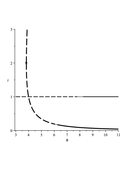
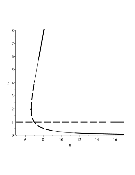
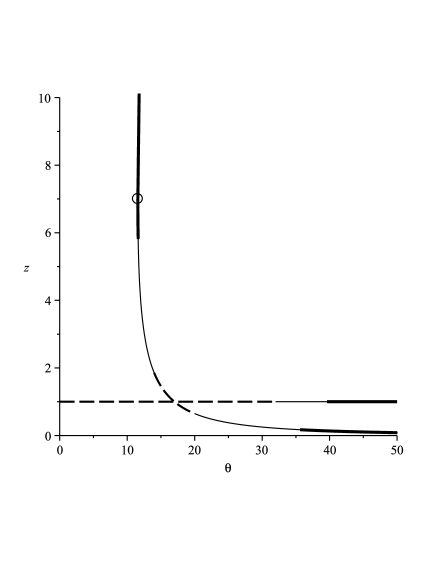
In Figure 1 the functions $z_{i}=x^{2}_{i}(m,\theta)$, $i=1,2$ are shown for $k=2$, $q=8$, $m=1,2,3$.

Figure 1. The graphs of the functions $z_{i}=z_{i}(m,\theta)$, $i=1,2$, for $k=2$, $q=8$ and $m=1,2,3$. The horizontal axis presents $\theta$ and the vertical axis presents $z_{i}$. Circle dots having coordinates $(\theta_{m},{q-m\over m})$, $m=1,2,3$ separate graph of $z_{1}$ from graph of $z_{2}$. The graph of $z_{2}(1,\theta)$ is the curve $I$. The graph of $z_{1}(1,\theta)$ is the curve $II$. $z_{2}(2,\theta)$ is $III$. $z_{1}(2,\theta)$ is $IV$, $z_{2}(3,\theta)$ is $V$. $z_{1}(3,\theta)$ is $VI$. The intersection point of $z_{1}$ functions has coordinate $(\theta_{c},1)=(9,1)$. For $m=4$ the graphs of the functions $z_{i}(4,\theta)$ are similar to the above given graphs, but the circle point separating them coincides with the point $(9,1)$ of the intersections, since $\theta_{\lfloor{8\over 2}\rfloor=4}=\theta_{c}=9$.

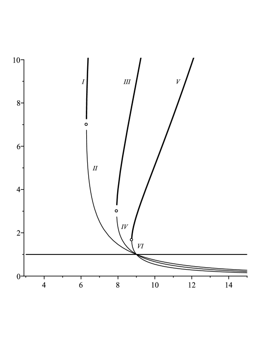
We have the following

Proposition 3.8.

• Each SGM of the model (3.4) corresponds to a solution $z_{x}\in R$, $x\in V$ of the following functional equation

  $$z_{x}=\prod_{y\in S(x)}{(\theta+m-1)z_{y}+q-m\over mz_{y}+q-m-1+\theta}.$$ (3.25)

• If $z_{x}$ is a solution of (3.25) then

  $$\min\{1,z_{1},z_{2}\}\leq z_{x}\leq\max\{1,z_{1},z_{2}\},$$ (3.26)

  where $z_{1}$, $z_{2}$ are solutions to (2.13).

Proof.

1. This was proved already below (3.13) using relations between boundary laws. One can also give a direct proof, as in [24, Theorem 2.1.].

2. For $z>0$ by Lemma 3.7 we have $a<g(z)<A$. Using this inequality from (3.25) we get

$$a^{k}<z_{x}<A^{k}.$$

Now we consider the function $g(z)$ on $[a^{k},A^{k}]$ and on this segment, using Lemma 3.7, we get the bounds $g(a^{k})<g(z)<g(A^{k})$. Then

$$(g(a^{k}))^{k}<z_{x}<(g(A^{k}))^{k}.$$

Iterating this argument we obtain

$$f_{m}^{n}(a^{k})<z_{x}<f_{m}^{n}(A^{k}),$$

where $f_{m}(z)$ is defined in (2.13), and $f_{m}^{n}$ is its $n$th iteration. It is easy to see that $\max\{1,z_{1},z_{2}\}\leq f_{m}^{n}(A^{k})$ and the sequence $a_{n}=f_{m}^{n}(A^{k})$ is decreasing. Indeed, by Lemma 3.7 the function $g$ is increasing, hence $f_{m}(z)=(g(z))^{k}$ is an increasing function too and $f_{m}$ is bounded by $A^{k}$, i.e., $f_{m}(z)<A^{k}$. Writing the last inequality for $z=A^{k}$ we get $a_{1}<A^{k}$. Since $f_{m}$ is an increasing function we obtain from the last inequality $a_{2}=f_{m}(a_{1})<f_{m}(A^{k})=a_{1}$, i.e. $a_{2}<a_{1}$. From this iterating $f_{m}$ again we get $a_{3}<a_{2}$ and so on. Thus the sequence $a_{n}$ has a limit $\alpha$, with $\alpha\geq\max\{1,z_{1},z_{2}\}$. This limit point must be a fixed point for $f_{m}$. But since the function $f_{m}$ has no fixed point in $(\max\{1,z_{1},z_{2}\},+\infty)$ we get that $\alpha=\max\{1,z_{1},z_{2}\}$. ∎

Let $\mathcal{G}(H^{\prime})$ the set of all SGMs of the model (3.4).

Denote

$$\theta_{m}(k)=1+{mx_{*}^{k}+q-m\over x_{*}^{k-1}+x_{*}^{k-2}+\dots+x_{*}},$$ (3.27)

where $x_{*}$ is the unique solution (see Step 3 in proof of Theorem 1 [14]) of the following equation

$$m\sum_{i=1}^{k-1}ix^{2k-i-1}-(q-m)\sum_{i=1}^{k-1}ix^{i-1}=0.$$ (3.28)

Theorem 3.9.

For the Ising model (3.4) on the Cayley tree of order $k\geq 2$ the following statements are true

• If $\theta<\theta_{m}(k)$ then there is unique TISGM $T(\mu_{0})$.

• If $\theta=\theta_{m}(k)$ or $\theta=\theta_{c}={q+k-1\over k-1}$ then there are 2 TISGMs $T(\mu_{0}),T(\mu_{1})$.

• If $\theta_{m}(k)<\theta\neq\theta_{c}$ then there are 3 TISGMs $T(\mu_{0}),T(\mu_{1}),T(\mu_{2})$. Moreover, at least two of these measures are extreme in $\mathcal{G}(H^{\prime})$.

Proof.

The measures $T(\mu_{i})$, $i=0,1,2$ correspond to the solutions $z_{0}=1$, $z_{1}$ and $z_{2}$ of (2.13).

(1) In case $\theta<\theta_{m}(k)$ the equation (2.13) has the unique solution $z=z_{0}=1$. Consequently, by part 2 of Proposition 3.8 we obtain that $z_{x}\equiv 1$ is a unique solution of (3.25). Thus $\mathcal{G}(H^{\prime})=\{T(\mu_{0})\}$.

(2) If $\theta=\theta_{m}(k)$ then $z_{1}=z_{2}$, i.e. there are only two TISGMs $T(\mu_{0}),T(\mu_{1})$; if $\theta=\theta_{c}={q+k-1\over k-1}$ then $z_{0}=z_{1}$ and there are again two TISGMs.

(3) If $\theta_{m}(k)<\theta\neq\theta_{c}$ then all solutions $z_{0}=1$, $z_{1}$ and $z_{2}$ of (2.13) are distinct. The extremality of two of these measures can be deduced using the minimality and maximality of the corresponding values of solutions. Assume that $z_{2}$ is the maximal solution and $T(\mu_{2})$ is non-extreme, with a decomposition

$$T(\mu_{2})=\int T(\mu)(\omega)\nu(d\omega).$$

Then for any vertex $x\in V$ we have

$$z_{2}=\int z_{x}(\omega)\nu(d\omega).$$ (3.29)

By (3.26) and Lemma 3.7 $z_{2}$ is an extreme point in the set of all solutions $z_{x}$, and so (3.29) holds if $z_{x}(\omega)=z_{2}$ for almost all $\omega$. Hence, $T(\mu_{2})$ is extreme. ∎

4. Conditions for non-extremality

Let us continue with the investigation of the coarse-grained chains $T(\mu)$ with a focus on criteria for non-extremality which are based on properties of the corresponding $2\times 2$-transition matrix as it depends on coupling strength of the Potts model, the block-size $m$ and the choice of a branch of the boundary law.

In the case of three solutions, we denote the middle solution by $z_{\rm mid}$, which is unique element of the following set

$$\{1,z_{1},z_{2}\}\setminus\{\min\{1,z_{1},z_{2}\},\max\{1,z_{1},z_{2}\}\}.$$

By Lemma 3.7, for $2m<q$ we have $z_{\rm mid}=\max\{1,z_{1}\}$.

Let $T(\mu_{\rm mid})$ be the TISGM which corresponds to $z_{\rm mid}$. Recall that $\mu_{i}$ is the TISGM of the Potts model which corresponds to the boundary law $z_{i}(m)$, for the branches $i=1,2$.

Define the following numbers:

$$\theta_{0}=1+q+2\sqrt{2m(q-m)},\ \ \hat{\theta}_{0}=1+(\sqrt{2}+1)q,$$

$$\widehat{\theta}=(\sqrt{2}-1)q+2m+1,\ \ \theta^{*}=1+(\sqrt{2}+1)q-2m.$$ (4.1)

Theorem 4.1.

Let $k=2$, $2m<q$. Then the following statements hold.

• If $\theta\geq q+1$ then $T(\mu_{\rm mid})=T(\mu_{0})$ and

  $$T(\mu_{0})\hbox{ is }\left\{\begin{array}[]{ll}{\rm extreme},\ \ \mbox{if}\ \ \theta\leq\theta_{0}\\[8.53581pt] {\rm non-extreme},\ \ \mbox{if}\ \ \theta>\hat{\theta}_{0};\end{array}\right.$$

• Assume one of the following conditions is satisfied:

  • $2\leq m\leq q/7$ and $\theta\in[\theta_{m},\widehat{\theta})$;

  • $\theta\in(\theta^{*},+\infty)$.

  Then $\mu_{1}(\theta,m)$ is non-extreme.

• Assume one of the following conditions is satisfied:

  • $2\leq m\leq q/7$ and $\theta\geq\theta_{m}$;

  • $q<7m$, $m\geq 2$ and $\theta\in(\widehat{\theta},+\infty)$.

  Then $\mu_{2}(\theta,m)$ is non-extreme.(See Fig.3-4)

• If $\theta_{m}\leq\theta<q+1$ then $T(\mu_{\rm mid})=T(\mu_{1})$. Moreover, if $q>85$ then for each $m\leq[{q\over 85}]$ there are two critical values $\bar{\theta},\,\bar{\bar{\theta}}\in(\theta_{m},q+1)$, with $\bar{\theta}<\bar{\bar{\theta}}$ such that $T(\mu_{1})$ is non-extreme if $\theta\in(\bar{\theta},\bar{\bar{\theta}})$. Moreover, $\bar{\theta},\bar{\bar{\theta}}$ are solutions to

  $$(\theta-1)^{3}-(\sqrt{2}-1)q(\theta-1)^{2}-2(2\sqrt{2}-1)m(q-m)(\theta-1)+2qm(q-m)=0.$$ (4.2)

Figure 2. The graphs of the functions $z_{i}=z_{i}(m,\theta)$, $i=1,2$, for $q=3$ and $m=1$. The circle dot having coordinate $(\theta_{1},2)$ separates graph of $z_{1}$ from graph of $z_{2}$. The bold curves correspond to regions of solutions where the corresponding TISGM is non-extreme. This figure corresponds to Part (ii), b) of Theorem 4.1.

Figure 3. The graphs of the functions $z_{i}=z_{i}(m,\theta)$, $i=1,2$, for $q=6$ and $m=2$. The circle dot having coordinate $(\theta_{2},2)$ separates graph of $z_{1}$ from graph of $z_{2}$. The bold lines correspond to regions of solutions where corresponding TISGM is non-extreme. The upper bold curve corresponds to part (iii), d) and the lower bold curve corresponds to part (ii), b) of Theorem 4.1.

Figure 4. The graphs of the functions $z_{i}=z_{i}(m,\theta)$, $i=1,2$, for $q=16$ and $m=2$. The circle dot having coordinate $(\theta_{2},7)$ separates graph of $z_{1}$ from graph of $z_{2}$. The bold lines correspond to regions of solutions where corresponding TISGM is non-extreme. The bold $z_{2}$ corresponds to Part (iii), c); Bold parts of $z_{1}$ correspond to Part (ii), a) (upper bold curve) and Part (ii), b) (lower bold curve) of Theorem 4.1.

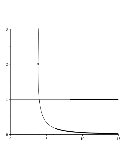
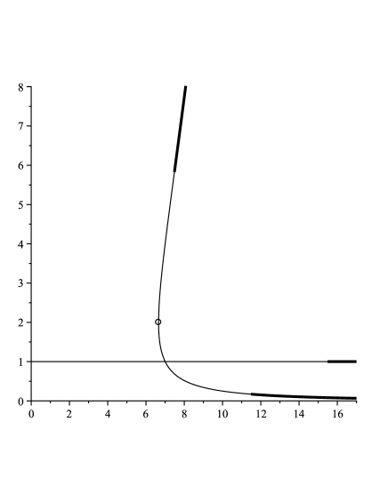
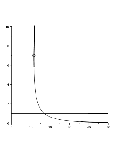
Proof.

(i) The equality $T(\mu_{\rm mid})=T(\mu_{0})$ follows from the second part of Lemma 3.7. To check the extremality we apply arguments used for the reconstruction on trees [5], [12], [17], [20], [21]. Consider Markov chains with states $\{1^{\prime},2^{\prime}\}$ and transition probabilities $p_{ij}$ defined by (3.3). It is known that a sufficient condition for non-extremality (which is equivalent to solvability of the associated reconstruction) of a Gibbs measure $T(\mu)$ corresponding to the matrix $T({\mathbb{P}})$ is that $k\lambda^{2}_{2}>1$, where $\lambda_{2}$ is the second largest (in absolute value) eigenvalue of $T({\mathbb{P}})$ [12]. On the other hand, Martin in [3] gives the following condition for extremality (non-reconstructibility)

$$k\left(\sqrt{T({\mathbb{P}})_{11}T({\mathbb{P}})_{22}}-\sqrt{T({\mathbb{P}})_{12}T({\mathbb{P}})_{21}}\right)^{2}\leq 1.$$

In case $z=1$ the matrix $T({\mathbb{P}})$ is

$$T({\mathbb{P}})={1\over\theta+q-1}\left(\begin{array}[]{cc}\theta+m-1&q-m\\[5.69054pt] m&\theta+q-m-1\end{array}\right).$$ (4.3)

Simple calculations show that above-mentioned conditions of extremality for $T(\mu_{0})$ (i.e. for the matrix (4.3)) are equivalent to the conditions on $\theta$ as mentioned in theorem.

(ii) Case $m\geq 2$.

Subcase: $\theta_{m}\leq\theta<q+1$. In this case by Lemma 3.7 we have $z_{1}>1$. By (3.24) (which requires $m\geq 2$) and Corollary 3.6 we have the second largest (in absolute value) eigenvalue of $\mathbb{P}$ is $a$ so to prove non-extremality we should check the Kesten-Stigum condition $2a^{2}>1$. Since $a>0$ the last inequality is equivalent to $\sqrt{2}a>1$. Denote

$$\gamma_{1}(\theta)=\sqrt{2}a-1=\sqrt{2}{(\theta-1)z_{1}\over(\theta+m-1)z_{1}+q-m}-1,$$

where

$$z_{1}=\left({\theta-1-\sqrt{(\theta-1)^{2}-4m(q-m)}\over 2m}\right)^{2}.$$

We have

$$\gamma_{1}^{\prime}(\theta)={\sqrt{2}(\theta-1)z_{1}\over((\theta+m-1)z_{1}+q-m)^{2}}\left(\sqrt{z_{1}}-{2(q-m)\over\sqrt{(\theta-1)^{2}-4m(q-m)}}\right)$$

$$=-\,{\sqrt{2z_{1}}(\theta-1)^{2}z_{1}\over((\theta+m-1)z_{1}+q-m)^{2}\sqrt{(\theta-1)^{2}-4m(q-m)}}.$$

Thus for any $\theta\geq\theta_{m}$ we have $\gamma_{1}^{\prime}(\theta)<0$. Hence $\gamma_{1}$ is a decreasing function of $\theta$. So to have $\sqrt{2}a>1$ it is necessary that

$$\gamma_{1}(\theta_{m})=\sqrt{2}{\sqrt{q-m}\over\sqrt{q-m}+\sqrt{m}}-1>0,$$

which is satisfied for $q\geq 7m$. Moreover, we have $\gamma_{1}(q+1)=-({\sqrt{2}-1\over\sqrt{2}})<0$. Consequently, there exists a unique $\theta=\widehat{\theta}$ such that $\gamma_{1}(\widehat{\theta})=0$. To find $\widehat{\theta}$ we solve $\gamma_{1}(\widehat{\theta})=0$ and by long (but simple) computations, using the explicit formula for $\gamma_{1}(\theta)$ and the expression for $z_{1}$ we get

$$\widehat{\theta}=(\sqrt{2}-1)q+2m+1.$$

Thus we proved that $2a^{2}>1$ iff $\theta<\widehat{\theta}$.

Subcase: $\theta\geq q+1$. In this case by Lemma 3.7 we have $z_{1}<1$ so by (3.24) and Corollary 3.6 we must check $2b^{2}>1$. Define

$$\xi_{1}(\theta)=\sqrt{2}b-1={(\theta-1)\sqrt{2z_{1}}\over(\theta+m-1)z_{1}+q-m}-1,$$

We have

$$\xi_{1}^{\prime}(\theta)={\sqrt{2z_{1}}(\theta-1)^{2}z_{1}\over((\theta+m-1)z_{1}+q-m)^{2}\sqrt{(\theta-1)^{2}-4m(q-m)}}>0.$$

Hence $\xi_{1}$ is an increasing function of $\theta$. Moreover, we have $\xi_{1}(q+1)=\gamma_{1}(q+1)=-({\sqrt{2}-1\over\sqrt{2}})<0$. Since $\xi_{1}(\theta)$ is increasing it is bounded from above by its limit for $\theta\to+\infty$. So we compute

$$\lim_{\theta\to\infty}\xi_{1}(\theta)=-1+\sqrt{2}\lim_{\theta\to\infty}{(\theta-1)\sqrt{z_{1}}\over(\theta+m-1)z_{1}+q-m}$$

$$=-1+\sqrt{2}\lim_{\theta\to\infty}{1\over\left({\theta+m-1\over\theta-1}\right)\sqrt{z_{1}}+{q-m\over(\theta-1)\sqrt{z_{1}}}}.$$ (4.4)

Using formula (2.16) we get

$$\lim_{\theta\to\infty}\sqrt{z_{1}}=\lim_{\theta\to\infty}{2(q-m)\over\theta-1+\sqrt{(\theta-1)^{2}-4m(q-m)}}=0.$$

$$\lim_{\theta\to\infty}(\theta-1)\sqrt{z_{1}}=\lim_{\theta\to\infty}{2(q-m)\over 1+\sqrt{1-{4m(q-m)\over(\theta-1)^{2}}}}=q-m.$$

Using these formulas we get from (4.4)

$$\lim_{\theta\to\infty}\xi_{1}(\theta)=\sqrt{2}-1>0.$$

Consequently, there exists a unique $\theta=\theta^{*}$ such that $\xi_{1}(\theta^{*})=0$. To find $\theta^{*}$ we solve $\xi_{1}(\theta^{*})=0$ and by simple computations using the explicit formula of $\xi_{1}(\theta)$ we get

$$\theta^{*}=1+(\sqrt{2}+1)q-2m.$$

Thus we proved that $2b^{2}>1$ if $\theta>\theta^{*}$.

Case $m=1$. In this case, as mentioned before (3.24) the second largest eigenvalue is $b$, therefore we have to check $\xi_{1}(\theta)=\sqrt{2}b-1>0$. We note that $\xi_{1}^{\prime}(\theta)>0$ for each $\theta\geq\theta_{m}$, and

$$\xi_{1}(\theta_{m})={\sqrt{2m}\over\sqrt{q-m}+\sqrt{m}}-1<0.$$

Hence again we have $\xi_{1}(\theta)>0$ iff $\theta\in(\theta^{*},+\infty)$.

(iii) Case $m\geq 2$. Since $z_{2}>1$ for any $\theta\geq\theta_{m}$, using (3.24) and Corollary 3.6 we shall check only $2a^{2}>1$. Denote

$$\gamma_{2}(\theta)=\sqrt{2}a-1=\sqrt{2}{(\theta-1)z_{2}\over(\theta+m-1)z_{2}+q-m}-1,$$

where

$$z_{2}=\left({\theta-1+\sqrt{(\theta-1)^{2}-4m(q-m)}\over 2m}\right)^{2}.$$

We have

$$\gamma_{2}^{\prime}(\theta)={\sqrt{2}(\theta-1)z_{2}\over((\theta+m-1)z_{2}+q-m)^{2}}\left(\sqrt{z_{2}}+{2(q-m)\over\sqrt{(\theta-1)^{2}-4m(q-m)}}\right)>0.$$

Thus for any $\theta\geq\theta_{m}$ we have $\gamma_{2}^{\prime}(\theta)>0$. Hence $\gamma_{2}$ is an increasing function of $\theta$. For $q\geq 7m$ we have

$$\gamma_{2}(\theta_{m})=\gamma_{1}(\theta_{m})>0.$$

Hence $\gamma_{2}(\theta)>0$ for all $\theta>\theta_{m}$. Consequently, $\mu_{2}$ is non-extreme.

In case $q\leq 6$ or $q\geq 7$ with $[q/7]<m$ we have $\gamma_{1}(\theta_{m})=\gamma_{2}(\theta_{m})<0$. Since $\gamma_{2}$ is an increasing function $\gamma_{2}(\theta)=0$ has a unique solution, which is equal to $\widehat{\theta}$. Thus $\gamma_{2}(\theta)>0$ for all $\theta>\widehat{\theta}$.

Case $m=1$. Define

$$\xi_{2}(\theta)=\sqrt{2}b-1={(\theta-1)\sqrt{2z_{2}}\over\theta z_{2}+q-1}-1.$$

We have

$$\xi_{2}^{\prime}(\theta)=-{\sqrt{2z_{2}}(\theta-1)^{2}z_{2}\over(\theta z_{2}+q-1)^{2}\sqrt{(\theta-1)^{2}-4(q-1)}}<0.$$

Hence $\xi_{2}$ is a decreasing function of $\theta$. Moreover, we have

$$\xi_{2}(\theta_{m})=\xi_{1}(\theta_{m})=-(1-{\sqrt{2}\over\sqrt{q-1}+1})<0.$$

Thus $\xi_{2}(\theta)<0$ for all $\theta\geq\theta_{m}$.

(iv) In this case the matrix $T({\mathbb{P}})$ is

$$T({\mathbb{P}})=\left(\begin{array}[]{cc}{(\theta+m-1)z\over Z_{1}}&{q-m\over Z_{1}}\\[8.53581pt] {mz\over Z_{2}}&{\theta+q-m-1\over Z_{2}}\end{array}\right),$$ (4.5)

which has eigenvalues $1$ and $\lambda_{2}(\hat{\mathbb{P}})$ given in (3.23). It is easy to check that

$$\theta-1-(\sqrt{z_{i}}-1)m\geq 0,\ \ i=1,2,$$

i.e. $\lambda_{2}(\hat{\mathbb{P}})>0.$

We define the following function

$$\eta_{1}(\theta)=\sqrt{2}{(\theta-1-(\sqrt{z_{1}}-1)m)z_{1}\over(\theta+m-1)z_{1}+q-m}-1.$$

We have

$$\eta_{1}(\theta_{m})=\eta_{1}(q+1)=-{\sqrt{2}-1\over\sqrt{2}}<0.$$

Using the explicit formulas for $z_{1}$ (given in Proposition 2.4) we note that $\eta_{1}(\theta)>0$ iff

$$\psi(\theta)=(\theta-1)^{3}-(\sqrt{2}-1)q(\theta-1)^{2}-2(2\sqrt{2}-1)m(q-m)(\theta-1)+2qm(q-m)<0.$$ (4.6)

It is well known (see [23, p.28]) that the number of positive roots of a polynomial does not exceed the number of sign changes of its coefficients. Using this fact one can see that the equation $\psi(\theta)=0$ has up to two positive roots denoted by $\bar{\theta},\bar{\bar{\theta}}$. Moreover $\psi^{\prime}(\theta)=0$ has the unique positive solution

$$\theta_{0}=1+{q\over 3}(\sqrt{2}-1)+{1\over 3}\sqrt{(3-2\sqrt{2})q^{2}+6(2\sqrt{2}-1)m(q-m)}.$$

Since $\theta>1$, $\psi(1)>0$ and $\psi(\infty)>0$ we have that at $\theta_{0}$ the function $\psi(\theta)$ has minimum. Therefore to have non-empty set of solutions for $\psi(\theta)<0$ it is necessary $\psi(\theta_{0})<0$. Maple solved $\psi(\theta_{0})=0$ with respect to $q$ and gave explicitly four solutions:

$$q=m,\ \ q=2m,\ \ q=m_{1},\ \ q=m_{2},$$

where $m_{1}$ is negative and $m_{2}$ is a linear function of $m$, i.e.,

$$m_{2}=\frac{14\left(14308\sqrt{2}+19845+288\sqrt{2}\sqrt{1055+746\sqrt{2}}+452\sqrt{1055+746\sqrt{2}}\right)}{4015+4768\sqrt{2}-1127\sqrt{1055+746\sqrt{2}}+833\sqrt{2}\sqrt{1055+746\sqrt{2}}}m.$$

We note that $m_{2}\approx 85m$. By our assumption $1\leq m\leq q/2$, the condition $\psi(\theta_{0})<0$ is equivalent to $q>m_{2}$. The last inequality holds for some $m$ (with $1\leq m\leq q/2$) if $q>85$. This completes the proof. ∎

Remark 4.2.

In the case $q=7$ the condition $q\geq 7m$ leaves only the value $m=1$. Then $\theta_{1}=1+2\sqrt{6}\approx 5.898979$ and $\widehat{\theta}=3+7(\sqrt{2}-1)\approx 5.899494$. Hence $\widehat{\theta}-\theta_{1}\approx 0.00051$.

5. Conditions for extremality

We turn our attention to sufficient conditions for extremality (or non-reconstructability in information-theoretic language) of the full chains of the Potts model, depending on coupling strength parameterized by $\theta$, the block size $m$ and the branch of the boundary law $z$.

Recall that by $\mu_{i}(\theta,m)$ we denote the TISGM which corresponds to the values of the boundary law $z_{i}(\theta,m)$, $i=1,2$, which is a solution to (2.13).

5.1. Main results of this section. Let us first give all main results of this section.

Recall $\theta_{1}=1+2\sqrt{q-1}$ (see (2.14)) and $\theta^{*}=1+(\sqrt{2}+1)q-2m$ (see (4.1)).

Theorem 5.1.

If $k=2$, $m=1$ then the following is true.

• • If $q=3,4,\dots,16$ then there exists $\theta^{**}$ such that $\theta_{c}=q+1<\theta^{**}<\theta^{*}$ and the measure $\mu_{1}(\theta,1)$ is extreme for any $\theta\in[\theta_{1},\theta^{**})$. Moreover $\theta^{**}$ is the unique positive solution of the following equation

    $$\theta^{3}-(q-3)\theta^{2}-(2q-7)\theta-(q+5)=0.$$

  • If $q\geq 17$ then there are $\bar{\theta}_{1},\bar{\theta}_{2}\in(\theta_{1},\theta_{c})$ such that $\bar{\theta}_{1}<\bar{\theta}_{2}$ and the measure $\mu_{1}(\theta,1)$ is extreme for any $\theta\in[\theta_{1},\bar{\theta}_{1})\cup(\bar{\theta}_{2},\theta^{**})$. Moreover $\bar{\theta}_{1},\bar{\theta}_{2}$ are positive solutions of the following equation

    $$\theta^{3}-(q-1)\theta^{2}-(2q-3)\theta+(4q^{2}-13q+11)=0.$$

• The measure $\mu_{2}(\theta,1)$ is extreme for any $\theta\geq\theta_{1}$, $q\geq 2$. (see Fig.6)

Remark 5.2.

We are considering the solution of the form $(\underbrace{z,z,\dots,z}_{m},1,\dots,1)$, but of course the results are true for any permutation of the coordinates of this solution. We note that $\mu_{2}(\theta,1)$ corresponds to $m=1$, by the permutations we get $q$ distinct measures similar to $\mu_{2}(\theta,1)$. These measures coincide with the well-known TISGMs considered in [6], because in [6] the author only used the maximal solutions $z_{2}$. Moreover in [6] it was proved that these measures are extreme as soon as they exist. Our proof (that is the proof of the part (b) of Theorem 5.1) is an alternative to the proof of [6]. Since the solutions $z_{1}=z_{1}(\theta,q,m)$ for $m\geq 1$ and $z_{2}=z_{2}(\theta,q,m)$ for $m\geq 2$ were not known before, the extreme measures $\mu_{1}(\theta,m)$, $\mu_{2}(\theta,m)$ corresponding to them which we constructed in our paper, are new.

The following theorem corresponds to the case: $m\geq 2$. From condition $2\leq m\leq[q/2]$ it follows that $q\geq 4$.

Theorem 5.3.

• Let $k=2$.

• If $m=2$ then the following is true.

  • For each $q=4,5,6,7,8$ there exists $\breve{\theta}>\theta_{c}=q+1$ such that the measure $\mu_{1}(\theta,2)$ is extreme for any $\theta\in[\theta_{2},\breve{\theta})$.

  • For each $q\geq 9$ there exists $\theta^{\dagger}\in(\theta_{2},q+1)$ such that the measure $\mu_{1}(\theta,2)$ is extreme for any $\theta\in[\theta^{\dagger},\breve{\theta})$, where $\theta^{\dagger}=\theta^{\dagger}(q)$ is the unique solution of

    $$\theta^{3}-(q+3)\theta^{2}+(6q-17)\theta-(9q-19)=0$$

    and $\breve{\theta}=\breve{\theta}(q)$ is the unique solution of

    $$\theta^{3}-(q+3)\theta^{2}-(2q-15)\theta-(q+13)=0.$$

• If $m=2$ then for each $q=4,5,6,7,8$ there exists $\grave{\theta}=\grave{\theta}(q)$ such that $\theta_{2}<\grave{\theta}\leq q+1$ and $\mu_{2}(\theta,2)$ is extreme for $\theta\in[\theta_{2},\grave{\theta})$ (see Fig.6).

• If $q<{m+1\over 2m}\left[3m+1+\sqrt{m^{2}+6m+1}\right]$ and $m\geq 2$ then the measure $\mu_{1}(\theta_{m},m)=\mu_{2}(\theta_{m},m)$ is extreme.

The following theorems are obtained by a continuity argument.

Theorem 5.4.

• Let $k=2$.

• For each $m\leq[q/2]$ there exists a neighborhood $U_{m}(\theta_{c})$ of $\theta_{c}$ such that the measure $\mu_{1}(\theta,m)$ is extreme if $\theta\in U_{m}(\theta_{c})$ (see Fig.7).

• If $m=1$ or condition (iii) of Theorem 5.3 is satisfied then there exists a neighborhood $V_{m}(\theta_{m})$ of $\theta_{m}$ such that measures $\mu_{i}(\theta,m),$ $i=1,2$ are extreme if $\theta\in V_{m}(\theta_{m})$.

Theorem 5.5.

For the ferromagnetic $q$-state Potts model (with $q\geq 3$) on the Cayley tree of order two, there exists a punctured neighborhood $U(\theta_{c})$ of $\theta_{c}$ such that there are at least $2^{q-1}+q$ extreme TISGMs for each $\theta\in U(\theta_{c})$.

Here the model is called ferromagnetic if $\theta>1$, and as usual a punctured neighborhood of $\theta_{c}$ is an open neighborhood from which the value $\theta_{c}$ was removed.

The proofs of these theorems follow after the following subsection.

Figure 5. The graphs of the functions $z_{i}=z_{i}(m,\theta)$, for $q=3$, $m=1$ and the graph of $z(\theta)\equiv 1$. The bold curves correspond to regions of solutions where the corresponding TISGM is non-extreme (corresponds to part (ii), b) of Theorem 4.1). The dashed bold curves correspond to regions of solutions where the corresponding TISGM is extreme (see parts (a) and (b) of Theorem 5.1). The gaps between the two types of curves are given by thin curves.

Figure 6. The graphs of the functions $z_{i}=z_{i}(m,\theta)$, for $q=6$, $m=2$ and the graph of $z(\theta)\equiv 1$. The types of curves corresponding to certain extremality and certain non-extremality are as in Fig.6 (corresponds to Theorem 5.3).

Figure 7. The graphs of the functions $z_{i}=z_{i}(m,\theta)$, for $q=16$, $m=2$ and the graph of $z(\theta)\equiv 1$. The types of curves are again as in Fig.6 (corresponds to part a) of Theorem 5.4).

5.2. Reconstruction insolvability on trees

We use a result of [18] to establish a bound for reconstruction insolvability corresponding to the matrix (channel) of a solution $z\neq 1$.

Let us first give some necessary definitions from [18]. For $k\geq 2$, let $\mathbb{T}^{k}$ denote a half tree, i.e., the infinite rooted $k$-ary tree (in which every vertex has $k$ children). Consider an initial finite complete subtree $\mathcal{T}$, that is a tree of the following form: in the rooted tree $\mathbb{T}^{k}$, take all vertices at distance $\leq d$ from the root, plus the edges joining them, where $d$ is a fixed constant. We identify subgraphs of $\mathcal{T}$ with their vertex sets and write $E(A)$ for the edges within a subset $A$ and $\partial A$ for the boundary of $A$, i.e., the neighbors of $A$ in $(\mathcal{T}\cup\partial\mathcal{T})\setminus A$.

In [18] the key ingredients are two quantities, $\kappa$ and $\gamma$, which bound the probabilities of percolation of disagreement down and up the tree, respectively. Both are properties of the collection of Gibbs measures $\{\mu^{\tau}_{{\mathcal{T}}}\}$, where the boundary condition $\tau$ is fixed and $\mathcal{T}$ ranges over all initial finite complete subtrees of $\mathbb{T}^{k}$. For a given subtree $\mathcal{T}$ of $\mathbb{T}^{k}$ and a vertex $x\in\mathcal{T}$, we write $\mathcal{T}_{x}$ for the (maximal) subtree of $\mathcal{T}$ rooted at $x$ that is a tree given by $\mathcal{T}\cap\mathbb{T}^{k}_{x}$, with $\mathbb{T}_{x}^{k}$ the half tree with root $x$. We draw the trees with the root at the top and the leaves at the bottom. When $x$ is not the root of $\mathcal{T}$, let $\mu_{\mathcal{T}_{x}}^{s}$ denote the (finite-volume) Gibbs measure in which the parent of $x$ has its spin fixed to $s$ and the configuration on the bottom boundary of ${\mathcal{T}}_{x}$ (i.e., on $\partial{\mathcal{T}}_{x}\setminus\{\mbox{parent\ \ of}\ \ x\}$) is specified by $\tau$.

For two measures $\mu_{1}$ and $\mu_{2}$ on $\Omega$, $\|\mu_{1}-\mu_{2}\|_{x}$ denotes the variation distance between the projections of $\mu_{1}$ and $\mu_{2}$ onto the spin at $x$, i.e.,

$$\|\mu_{1}-\mu_{2}\|_{x}={1\over 2}\sum_{i=1}^{q}|\mu_{1}(\sigma(x)=i)-\mu_{2}(\sigma(x)=i)|.$$

Denote by $\Omega^{\tau}_{\mathcal{T}}$ the set of configurations $\sigma$ given on $\mathcal{T}\cup\partial\mathcal{T}$ that agree with $\tau$ on $\partial\mathcal{T}$, i.e., $\tau$ specifies a boundary condition on $\mathcal{T}$. For any $\eta\in\Omega^{\tau}_{\mathcal{T}}$ and any subset $A\subseteq\mathcal{T}$, the Gibbs distribution on $A$ conditional on the configuration outside $A$ being $\eta$ is denoted by $\mu^{\eta}_{A}$.

Let $\eta^{x,s}$ be the configuration $\eta$ with the spin at $x$ set to $s$.

Let $\mathbb{P}=(P_{ij})$ be a channel on $\mathbb{T}^{k}$, and $\mu$ its associated Gibbs measure. Following [18, page 165] define

$$\kappa={1\over 2}\max_{i,j}\sum_{l}|P_{il}-P_{jl}|;$$ (5.1)

$$\gamma\equiv\gamma(\mu)=\sup_{A\subset\mathbb{T}^{k}}\max\|\mu^{\eta^{y,s}}_{A}-\mu^{\eta^{y,s^{\prime}}}_{A}\|_{x},$$

where the supremum is taken over all subsets $A\subset\mathbb{T}^{k}$, the maximum is taken over all boundary conditions $\eta$, all sites $y\in\partial A$, all neighbors $x\in A$ of $y$, and all spins $s,s^{\prime}\in\{1,\dots,q\}$.

As the main ingredient we apply [18, Theorem 9.3], which is

Theorem 5.6.

For an arbitrary (ergodic and permissive) channel ${\mathbb{P}}=(P_{ij})_{i,j=1}^{q}$ on a tree, the reconstruction of the corresponding tree-indexed Markov chain is impossible if $k\kappa\gamma<1$.

We note that the above mentioned results of [18] are given for a rooted Cayley tree (half tree $\mathbb{T}^{k}$). The following lemma says that the results can be extended for unrooted Cayley tree (full tree $\Gamma^{k}$).

Lemma 5.7.

Consider a tree-indexed Markov chain with a given fixed transition matrix $(P_{ij})$ on two different graphs: First, a Cayley tree where every vertex has $k+1$ nearest neighbors. Second, a rooted tree where only the root has $k$ nearest neighbors and all other vertices have $k+1$ neighbors. Then the chain on the rooted tree is reconstructable if and only if the chain on the Cayley tree is reconstructable.

Proof.

Let us denote by $\rho^{i}_{n}$ the joint probability distribution of the spins $\{\sigma^{i}(v):v\in V,\,d(x_{0},x)=n\}$ which are at the boundary at distance $n$ to the root $x_{0}$ on the rooted tree, this is obtained by sending a symbol $i$ from the root $x_{0}$ using the transition matrix of the Markov chain. It is well known that the chain is non-reconstructable if and only if, for any pair of different symbols $i,j\in\{1,\dots,q\}$, the relative entropy vanishes in the large-$n$ limit, that is we have

$$\lim_{n\rightarrow\infty}S(\rho^{i}_{n}|\rho^{j}_{n})=0.$$

(For more background on this, see Propositions 14 and 15 on page 295 of [22]).

We will show that non-reconstructability on the rooted tree (the root has $k$ adjacent vertices, the half tree) implies non-reconstructability on the Cayley tree (the root has $k+1$ adjacent vertices, the full tree). The other direction is obvious. To do so, we consider the Cayley tree and single out a vertex $x_{0}$ which we will call the root. Let us label its nearest neighbors by $v_{1},\dots,v_{k},v_{k+1}$. The boundary at distance $n$ for the Cayley tree decomposes into a first part which is connected to the root $x_{0}$ via the vertices $v_{1},\dots,v_{k}$ and a second part of those vertices which is connected to $x_{0}$ via $v_{k+1}$. We denote the spin distributions corresponding to this decomposition of boundary vertices by $\rho^{i,<}_{n}$ and $\rho^{i,>}_{n}$, and their joint distribution by $\rho^{i,\text{full}}_{n}$. By the Markov property of the chain the spins on these two parts of the boundary are mutually independent and we can write $\rho^{i,\text{full}}_{n}=\rho^{i,<}_{n}\times\rho^{i,>}_{n}$. As a consequence we have for the relative entropy between measures on the full boundary which are obtained by sending $i\neq j$ that

$$S(\rho^{i,\text{full}}_{n}|\rho^{j,\text{full}}_{n})=S(\rho^{i,<}_{n}|\rho^{j,<}_{n})+S(\rho^{i,>}_{n}|\rho^{j,>}_{n}).$$ (5.2)

We recognize that $\rho^{i,<}_{n}$ is the distribution of boundary sites on the rooted tree where the root has $k$ children. Noting that $\rho^{i,>}_{n}$ is the distribution of boundary sites on a tree where the root has one child, and all other sites have $k$ children, we use the recursion from root to boundary to write $\rho^{i,>}_{n}=\sum_{a=1}^{q}P_{i,a}\rho^{a,<}_{n-1}$ as a sum over the spin-value $a$ of the single vertex $v_{k+1}$ at distance $1$ to the root. Here $\rho^{a,<}_{n-1}$ is the distribution of the boundary sites at distance $n-1$ from $v_{k+1}$ obtained by sending the letter $a$. By convexity of the relative entropy in both arguments we get

$$S(\rho^{i,>}_{n}|\rho^{j,>}_{n})\leq\sum_{a,b}P_{i,a}P_{j,b}S(\rho^{a,<}_{n-1}|\rho^{b,<}_{n-1}).$$ (5.3)

By (5.2) and (5.3) we see now that non-reconstruction on the smaller tree, and hence $\lim_{n\rightarrow\infty}S(\rho^{i,<}_{n}|\rho^{j,<}_{n})=0$ for all $i\neq j$, implies that $\lim_{n\rightarrow\infty}S(\rho^{i,\text{full}}_{n}|\rho^{j,\text{full}}_{n})=0$ for all $i\neq j$, and hence non-reconstruction on the larger tree. ∎

It is easy to see that the channel ${\mathbb{P}}$ corresponding to a TISGM of the Potts model is ergodic and permissive. Thus by Theorem 5.6 and Lemma 5.7 the criterion of extremality of a TISGM is $k\kappa\gamma<1$.

The constant $\gamma$ does not have a clean general formula, but can be estimated in specific models (as Ising, Hard-Core etc.). For example, if ${\mathbb{P}}$ is the channel of the Potts model then (see Theorem 8.1 in page 160 of [18]):

$$\gamma\leq{\theta-1\over\theta+1}.$$ (5.4)

Below we shall use this inequality. Consider the case $z\neq 1$ (where $z=x^{2}$ and $z$ is a solution to (2.13)), fix a solution of (2.12), which has the form $(\underbrace{z,z,\dots,z}_{m},1,\dots,1)$ and the corresponding matrix ${\mathbb{P}}$ given by (3.2). We shall now compute the constant $\kappa$. Recall matrix $\mathbb{P}$ given in (3.2) and $Z_{1}$, $Z_{2}$ given after formula (3.2). Since $z$ is a solution to (2.13) we have $Z_{1}=\sqrt[k]{z}Z_{2}$. Using this formula and (3.2) we get

$${1\over 2}\sum_{l=1}^{q}|P_{il}-P_{jl}|=\left\{\begin{array}[]{lll}a,\ \ \ \ \mbox{if}\ \ i,j=1,\dots,m\\[8.53581pt] b,\ \ \ \ \mbox{if}\ \ i,j=m+1,\dots,q\\[8.53581pt] c,\ \ \mbox{otherwise},\end{array}\right.$$

where $a$ and $b$ are defined in (3.23) and

$$c={1\over 2Z_{1}}\Big{(}z|\theta-\sqrt[k]{z}|+|1-\theta\sqrt[k]{z}|+(z(m-1)+q-m-1)|1-\sqrt[k]{z}|\Big{)}.$$ (5.5)

Hence we arrive at

$$\kappa=\left\{\begin{array}[]{ll}\max\{b,c\},\ \ \mbox{if}\ \ m=1\\[8.53581pt] \max\{a,b,c\}\ \ \mbox{if}\ \ m\geq 2.\end{array}\right.$$ (5.6)

5.3. Proof of Theorem 5.1

Proof.

Write the equation (2.13) for $k=2$, $m=1$ (the conditions of theorem). First take the square root on both sides, then obtain a cubic equation for $\sqrt{z}$ which by dividing out the solution $\sqrt{z}=1$ can be simplified to $z-(\theta-1)\sqrt{z}+q-1=0.$ For the solutions $\sqrt{z_{1}}$, $\sqrt{z_{2}}$ of the last equation one has $\sqrt{z_{1}}+\sqrt{z_{2}}=\theta-1$. Using this equality we get

$$\sqrt{z_{1}}\leq\sqrt{z_{1}}+\sqrt{z_{2}}=\theta-1<\theta.$$

Similarly, one gets $\theta>\sqrt{z_{2}}$. From these inequalities it follows that $|\theta-\sqrt{z_{i}}|=\theta-\sqrt{z_{i}}$. Since $\theta>1$ for $z_{i}\geq 1$ we get

$$|1-\theta\sqrt{z_{i}}|=\theta\sqrt{z_{i}}-1,\ \ |1-\sqrt{z_{i}}|=\sqrt{z_{i}}-1.$$

We can simplify the expression for $c$ (see (5.5), for $k=2$, $m=1$) using the above mentioned equalities for the absolute values present in $c$ and, using that $z_{i}$ is a solution to $z-(\theta-1)\sqrt{z}+q-1=0$ (i.e. replacing $z$ by $(\theta-1)\sqrt{z}-q+1$), finally we obtain

$$c={1\over Z_{1}}\left((\theta+q-2)\sqrt{z_{i}}-(q-1)\right).$$ (5.7)

Recall $b={(\theta-1)\sqrt{z_{i}}\over Z_{1}}$ (see (3.23)). For $z_{i}\geq 1$, using $b$ and $c$ given by (5.7) it is straightforward to see that $b\leq c$ (with equality if and only if $z_{i}=1$). Consequently, using (5.6) under condition $m=1$ we get $\kappa=c$.

(a) Case: $z_{1}\geq 1$. For $\theta\in[\theta_{1},\theta_{c}]=[1+2\sqrt{q-1},q+1]$ we have $z_{1}\geq 1$. By (5.4) and $\kappa=c$ we have

$$2\gamma\kappa\leq 2c{\theta-1\over\theta+1}={2(\theta-1)((\theta+q-2)\sqrt{z_{1}}-(q-1))\over(\theta z_{1}+q-1)(\theta+1)}.$$

Thus, to check $2\gamma\kappa<1$ it is sufficient to check

$${2(\theta-1)((\theta+q-2)\sqrt{z_{1}}-(q-1))\over(\theta z_{1}+q-1)(\theta+1)}<1.$$ (5.8)

Since $z_{1}$ is a solution to $z-(\theta-1)\sqrt{z}+q-1=0$ we can replace in (5.8) $z_{1}$ by $(\theta-1)\sqrt{z_{1}}-q+1$, simplify and put

$$\sqrt{z_{1}}={\theta-1-\sqrt{(\theta-1)^{2}-4(q-1)}\over 2}.$$

Then denoting

$$\psi_{1}(\theta)=(\theta-1)(\theta^{2}-\theta+6-4q)-(\theta^{2}-\theta+4-2q)\sqrt{(\theta-1)^{2}-4(q-1)}$$

we obtain that the inequality (5.8) is equivalent to $\psi_{1}(\theta)>0$, $\theta\in[\theta_{1},\theta_{c})$.

By $(\theta-1)^{2}>4(q-1)$, i.e. $\theta>\theta_{1}$ we get

$$\theta^{2}-\theta+6-4q>0,\ \ \theta^{2}-\theta+4-2q>0.$$

Using these inequalities the inequality $\psi_{1}(\theta)>0$ can be simplified to

$$u(\theta)=\theta^{3}-(q-1)\theta^{2}-(2q-3)\theta+(4q^{2}-13q+11)>0,\ \ \theta\in[\theta_{1},\theta_{c}].$$ (5.9)

The function $u(\theta)$ for $\theta\in(0,\theta_{c})$ has a minimum at $\bar{\theta}=\bar{\theta}(q)=(q-1+\sqrt{q^{2}+4q-8})/3$. Now we calculate the minimal value $u(\bar{\theta})$. Since $\bar{\theta}$ is a solution to

$$u^{\prime}(\theta)=3\theta^{2}-2(q-1)\theta-(2q-3)=0$$

in $u(\bar{\theta})$ we replace $\bar{\theta}^{2}$ by $(1/3)(2(q-1)\bar{\theta}+(2q-3))$ (in this way we reduce the powers of $\bar{\theta}$). We also replace $\bar{\theta}^{3}$ by $(\bar{\theta}/3)(2(q-1)\bar{\theta}+(2q-3))$ and simplifying $u(\bar{\theta})$ we get

$$u(\bar{\theta})=(8-4q-q^{2})\bar{\theta}+(48-56q+17q^{2}).$$

Now using the formula of $\bar{\theta}$ from the last equality we get

$$u(\bar{\theta})=-q^{3}+48q^{2}-156q+136-(q^{2}+4q-8)^{3/2}.$$ (5.10)

From (5.10) we obtain $u(\bar{\theta})>0$ iff $q=3,4,\dots,16$. Consequently, $u(\theta)\geq u(\bar{\theta})>0$ (i.e. $\psi_{1}(\theta)>0$) and $\mu_{1}(\theta,1)$ is extreme for all $\theta\in[1+2\sqrt{q-1},q+1]$, $q=3,4,\dots,16$.

For $q\geq 17$, using the explicit formulas for $\theta_{1},\bar{\theta},\theta_{c}$, one gets $\theta_{1}<\bar{\theta}<\theta_{c}$ and $u(\bar{\theta})<0$. Also we have

$$u(\theta_{1})=4(q+2\sqrt{q-1})>0,\ \ u(\theta_{c})=4((q-1)^{2}+3)>0.$$

Consequently, the equation $u(\theta)=0$ has two solutions $\bar{\theta}_{1}$ and $\bar{\theta}_{2}$ such that

$$\theta_{1}<\bar{\theta}_{1}<\bar{\theta}<\bar{\theta}_{2}<\theta_{c}.$$

Thus $u(\theta)>0$ and the measure $\mu_{1}(\theta,1)$ is extreme for any $\theta\in[\theta_{1},\bar{\theta}_{1})\cup(\bar{\theta}_{2},q+1].$

Case: $z_{1}<1$. In this case, using the explicit formula for $\sqrt{z_{1}}$ and the condition $\theta>\theta_{1}$ we get $\theta\sqrt{z_{1}}>1$. Indeed, this inequality is equivalent to $(q-2)\theta^{2}+\theta+1>0$, which holds for any $\theta>1$. Consequently, using $\theta>\sqrt{z_{1}}$, $\theta\sqrt{z_{1}}>1$ and $z_{1}<1$ from formula (5.5) for $m=1$, for all possible values of $q\geq 2$ we get

$$c={1\over Z_{1}}(\theta\sqrt{z_{1}}-1).$$

Recall again $b={(\theta-1)\sqrt{z_{1}}\over Z_{1}}$. Then

$$b\geq c\ \ \Leftrightarrow{(\theta-1)\sqrt{z_{1}}\over Z_{1}}\geq{1\over Z_{1}}(\theta\sqrt{z_{1}}-1)\ \ \Leftrightarrow(\theta-1)\sqrt{z_{1}}\geq\theta\sqrt{z_{1}}-1\ \ \Leftrightarrow\sqrt{z_{1}}\leq 1.$$

Thus if $z_{1}\leq 1$, i.e., $\theta\in(\theta_{c},+\infty)$ then $b\geq c$. Consequently, $\kappa=b$. So we have

$$2\gamma\kappa\leq 2b\cdot{\theta-1\over\theta+1}.$$

Hence it suffices to check

$$2b\cdot{\theta-1\over\theta+1}={2(\theta-1)^{2}\sqrt{z_{1}}\over(\theta+1)(\theta z_{1}+q-1)}<1.$$ (5.11)

Since $z_{1}$ is a solution to $z_{1}-(\theta-1)\sqrt{z_{1}}+q-1=0$, replacing $z_{1}$ by $(\theta-1)\sqrt{z_{1}}-q+1$ and using the explicit formula for $\sqrt{z_{1}}$ the inequality (5.11) becomes after some simplifications

$$f(\theta)=\theta^{3}-(q+3)\theta^{2}-(2q-7)\theta-(q+5)<0.$$

Using the Descartes rule (compare part (iv) of Theorem 4.1) for $f(\theta)$ we see that the equation $f(\theta)=0$ has at most one positive solution. Moreover, for any $q\geq 3$ we have $f(q+1)=-4q^{2}<0$. Now we show that $f(\theta^{*})>0$, where $\theta^{*}=(\sqrt{2}+1)q-1$ (see (4.1) for $m=1$). Indeed, we have

$$Q(q)\equiv f(\theta^{*})=(4+3\sqrt{2})q^{3}-6(3+2\sqrt{2})q^{2}+16(1+\sqrt{2})q-16$$

and

$$Q^{\prime}(q)=3(4+3\sqrt{2})q^{2}-12(3+2\sqrt{2})q+16(1+\sqrt{2}).$$

The equation $Q^{\prime}(q)=0$ has two positive solutions:

$$q_{\pm}={2\over 3}\cdot{9+6\sqrt{2}\pm\sqrt{33+24\sqrt{2}}\over 4+3\sqrt{2}}.$$

We have $q_{-}<q_{+}<3$. Therefore $Q(q)$ is an increasing function of $q\geq 3$. Consequently, for any $q\geq 3$ we have

$$Q(q)\geq Q(3)=21\sqrt{2}-22>0.$$

So there exists a unique $\theta^{**}$ with $q+1<\theta^{**}<\theta^{*}$ such that $f(\theta^{**})=0$. Thus $f(\theta)<0$ and $\mu_{1}(\theta,1)$ is extreme for $\theta\in[q+1,\theta^{**})$. Summarizing the results for the cases $z_{1}\geq 1$ and $z_{1}<1$ we get assertion (a).

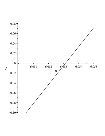
For $q=3$ a numerical analysis shows that $\theta^{**}\approx 6.053$. So $\theta^{*}-\theta^{**}=0.1896$ (see Fig.8). This is the length of the gap between the Kesten-Stigum threshold beyond which non-extremality certainly holds and our bound below which extremality certainly holds.

Figure 8. The graph of the function $f(\theta)$, for $q=3$, given in the interval $[6.05,6.055]$ indicates that the solution of $f(\theta^{**})=0$ is $\theta^{**}\approx 6.053$.

(b) For $\theta\geq\theta_{1}=1+2\sqrt{q-1}$ we have $z_{2}>1$, i.e $z_{2}$ is larger than $1$ as soon as it exists. Similarly as the case (a) we shall check $2c{\theta-1\over\theta+1}<1$. Denoting

$$\psi_{2}(\theta)=(\theta-1)(\theta^{2}-\theta+6-4q)+(\theta^{2}-\theta+4-2q)\sqrt{(\theta-1)^{2}-4(q-1)}$$

and using the fact that $z_{2}$ is a solution to $z_{2}-(\theta-1)\sqrt{z_{2}}+q-1=0$, replacing $z_{2}$ by $(\theta-1)\sqrt{z_{2}}-q+1$ and using the explicit formula

$$\sqrt{z_{2}}={\theta-1+\sqrt{(\theta-1)^{2}-4(q-1)}\over 2}$$

after simplifications we get that the last inequality is equivalent to $\psi_{2}(\theta)>0$, $\theta\geq\theta_{1}$. Note that

$$\theta^{2}-\theta+6-4q\leq\theta^{2}-\theta+4-2q,$$

so if we prove that

$$\theta^{2}-\theta+6-4q>0$$ (5.12)

then it follows that $\psi_{2}(\theta)>0$. Since $\theta>1$ the inequality (5.12) is equivalent to $\theta>(1+\sqrt{16q-23})/2$. Moreover, one can easily check that

$$(1+\sqrt{16q-23})/2<1+2\sqrt{q-1}=\theta_{1}$$

Thus we proved that $\psi_{2}(\theta)>0$ and $\mu_{2}(\theta,1)$ is extreme for any $\theta\geq 1+2\sqrt{q-1}$. ∎

5.4. Proof of Theorem 5.3

Proof.

Write the equation (2.13) for $k=2$, first take the square root on both sides, then obtain a cubic equation for $\sqrt{z}$ which by dividing out the solution $\sqrt{z}=1$ can be simplified to $mz-(\theta-1)\sqrt{z}+q-m=0.$ Using the fact that $z_{i}$ is a solution to $mz-(\theta-1)\sqrt{z}+q-m=0$ we simplify the expression of $c$ given in (5.5) for $m\geq 2$ and $z=z_{i}\geq 1$, $i=1,2$. For the solutions $\sqrt{z_{1}}$, $\sqrt{z_{2}}$ of the last equation one has $\sqrt{z_{1}}+\sqrt{z_{2}}={\theta-1\over m}$. Using this equality we get

$$\sqrt{z_{1}}\leq\sqrt{z_{1}}+\sqrt{z_{2}}={\theta-1\over m}<\theta.$$

Similarly, one gets $\theta>\sqrt{z_{2}}$. From these inequalities it follows that $|\theta-\sqrt{z_{i}}|=\theta-\sqrt{z_{i}}$. Since $\theta>1$ for $z_{i}\geq 1$ we get

$$|1-\theta\sqrt{z_{i}}|=\theta\sqrt{z_{i}}-1,\ \ |1-\sqrt{z_{i}}|=\sqrt{z_{i}}-1.$$

Consequently, repeatedly replacing $z_{i}$ in $c$ by $(1/m)((\theta-1)\sqrt{z_{i}}-q+m)$ and simplifying we obtain

$$c={1\over m^{2}Z_{1}}\left(\{m(\theta^{2}-\theta+q-m)-(\theta-1)^{2}\}\sqrt{z_{i}}-\{(m-1)\theta+1\}(q-m)\right).$$

Recall $a={(\theta-1)z_{i}\over Z_{1}}$ (see (3.23)) and by (3.24) for $z_{i}>1$ we have $b<a$. Now we shall check that $a>c$: replacing $z_{i}$ in $a$ by $(1/m)((\theta-1)\sqrt{z_{i}}-q+m)$ we get the following sequence of equivalent inequalities

$$a>c\ \ \Leftrightarrow\ \ {(\theta-1)((\theta-1)\sqrt{z_{i}}-q+m)\over mZ_{1}}\ \ >$$

$${\{m(\theta^{2}-\theta+q-m)-(\theta-1)^{2}\}\sqrt{z_{i}}-\{(m-1)\theta+1\}(q-m)\over m^{2}Z_{1}}\ \ \Leftrightarrow$$

$$[(m+1)(\theta-1)^{2}-m(\theta^{2}-\theta+q-m)]\sqrt{z_{i}}+(m-1)(q-m)(\theta-1)>0\Leftrightarrow$$

$$[\theta^{2}-(m+2)\theta-m(q-m-1)+1]\sqrt{z_{i}}+(m-1)(q-m)(\theta-1)>0.$$

To show that the last inequality is true for any $\theta>\theta_{m}$ it suffices to prove that

$$\theta^{2}-(m+2)\theta-m(q-m-1)+1>0.$$ (5.13)

This quadratic inequality (with respect to $\theta>1$) is true for any

$$\theta>1+{1\over 2}m+{1\over 2}\sqrt{4mq-3m^{2}}.$$

Now if we prove that

$$1+{1\over 2}m+{1\over 2}\sqrt{4mq-3m^{2}}<\theta_{m}=1+2\sqrt{m(q-m)}$$ (5.14)

then it follows that (5.13) holds for any $\theta>\theta_{m}$. So let us check (5.14):

$$(\ref{akc})\ \ \Leftrightarrow\ \ m+\sqrt{4mq-3m^{2}}<4\sqrt{m(q-m)}\ \ \Leftrightarrow$$

$$m^{2}+2m\sqrt{4mq-3m^{2}}+4mq-3m^{2}<16mq-16m\ \ \Leftrightarrow\sqrt{4mq-3m^{2}}<m+6q-8\ \ \Leftrightarrow$$

$$3q(3q-8)+(m-2)^{2}+2mq+12>0.$$

The last inequality is true for any $q\geq 2$. Thus we proved that

$$\kappa=\max\{a,b,c\}=a,\ \ \mbox{if}\ \ z_{i}>1.$$ (5.15)

(i) Case: $z_{1}\geq 1$. If $z=z_{1}\geq 1$, i.e. $\theta\in[\theta_{m},\theta_{c}]$ then as shown above we have $\kappa=a$. Hence

$$2\gamma\kappa\leq 2a{\theta-1\over\theta+1}={2(\theta-1)^{2}z_{1}\over((\theta+m-1)z_{1}+(q-m))(\theta+1)}.$$

Thus to check $2\gamma\kappa\leq 1$ it suffices to show

$${2(\theta-1)^{2}z_{1}\over((\theta+m-1)z_{1}+(q-m))(\theta+1)}<1.$$ (5.16)

The last inequality can be written as

$$[-\theta^{2}+(m+4)\theta+m-3]z_{1}+(\theta+1)(q-m)>0.$$ (5.17)

Replacing $z_{1}$ in (5.17) by $(1/m)((\theta-1)\sqrt{z_{1}}-q+m)$ we get

$$[-\theta^{2}+(m+4)\theta+m-3]((\theta-1)\sqrt{z_{1}}-q+m)+m(\theta+1)(q-m)>0.$$ (5.18)

By formula of $\sqrt{z_{1}}$ (see (2.16)) we have

$$\sqrt{z_{1}}={\theta-1-\sqrt{(\theta-1)^{2}-4m(q-m)}\over 2m}$$

$$={\left(\theta-1-\sqrt{(\theta-1)^{2}-4m(q-m)}\right)\left(\theta-1+\sqrt{(\theta-1)^{2}-4m(q-m)}\right)\over 2m\left(\theta-1+\sqrt{(\theta-1)^{2}-4m(q-m)}\right)}$$

$$={2(q-m)\over\theta-1+\sqrt{(\theta-1)^{2}-4m(q-m)}}.$$ (5.19)

Using formula (5.19) of $\sqrt{z_{1}}$ we obtain from (5.18)

$$-\theta^{3}+(2m+5)\theta^{2}-7\theta-(2m-3)+(\theta^{2}-4\theta+3)\sqrt{(\theta-1)^{2}-4m(q-m)}>0.$$ (5.20)

We note that

$$-\theta^{3}+(2m+5)\theta^{2}-7\theta-(2m-3)=(\theta-1)[-\theta^{2}+(2m+4)\theta+2m-3],$$

$$\theta^{2}-4\theta+3=(\theta-1)(\theta-3).$$

Using these equalities and dividing both side of (5.20) by $-(\theta-1)$ we get

$$\theta^{2}-(2m+4)\theta-2m+3-(\theta-3)\sqrt{(\theta-1)^{2}-4m(q-m)}<0.$$ (5.21)

For $m=2$ from (5.21) we obtain

$$\theta^{2}-8\theta-1-(\theta-3)\sqrt{(\theta-1)^{2}-8(q-2)}<0.$$ (5.22)

Subcase $\theta^{2}-8\theta-1\leq 0$. Since $\theta\geq\theta_{2}=1+2\sqrt{2(q-2)}>3$, the inequality (5.22) holds if $\theta^{2}-8\theta-1\leq 0$. From the last inequality we get $\theta\leq 4+\sqrt{17}$. Hence we should find $q\geq 4$ such that $1+2\sqrt{2(q-2)}\leq 4+\sqrt{17}$, i.e. $q\leq 8$. Then for $q<8$ we have $q+1<4+\sqrt{17}$ and the inequality (5.22) holds for $\theta$ satisfying

$$1+2\sqrt{2(q-2)}\leq\theta\leq 4+\sqrt{17}.$$

For $q=8$ we have

$$1+2\sqrt{2(q-2)}\leq\theta\leq 4+\sqrt{17}<q+1=9.$$

Thus we proved that the measure $\mu_{1}(\theta,2)$ is extreme

• if $q<8$ and $\theta\in[\theta_{2},q+1]$

• if $q=8$ and $\theta\in[\theta_{2},4+\sqrt{17}]$.

So, for $q=8$ we should check the inequality (5.22) for $\theta\in(4+\sqrt{17},9]$, since for such $\theta$ we have $\theta^{2}-8\theta-1>0$. This verification is included in the following subcase.

Subcase $\theta^{2}-8\theta-1>0$. In this case we have $\theta>4+\sqrt{17}$ which, together with $\theta>\theta_{2}$, gives that we should consider $q\geq 8$. Rewrite (5.22) as

$$\theta^{2}-8\theta-1<(\theta-3)\sqrt{(\theta-1)^{2}-8(q-2)}.$$

Take the square on both sides and simplify up to

$$\varphi(\theta,q)=\theta^{3}-(q+3)\theta^{2}+(6q-17)\theta-(9q-19)>0.$$

First let us check this inequality for $q=8$ and $\theta\in[4+\sqrt{17},9]$. The graph of the function $\varphi(\theta,8)$ is given in Figure 9. Thus we obtain that $\varphi(\theta,8)>0$ and $\mu_{1}(\theta,2)$ is extreme for $q=8$ on $[4+\sqrt{17},9]$ too. Summarizing the results of the previous subcase with the present one, we obtain that this measure is extreme on $[\theta_{2},q+1]$ for any $q\leq 8$.

Figure 9. The graph of the function $\varphi(\theta,q)$, for $q=8$ and $\theta\in[4+\sqrt{17},9]$.

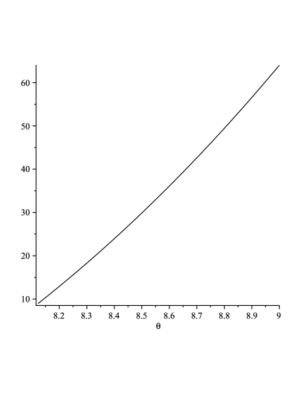
Now we shall consider the case $q\geq 9$. The equation $\varphi^{\prime}(\theta,q)=0$ has two solutions:

$$q_{\pm}={1\over 3}\cdot(q+3\pm\sqrt{q^{2}-12q+60}).$$

Since the coefficient of $\theta^{3}$ in $\varphi$ is positive (=1), the function has a maximum at $q_{-}$ and a minimum at $q_{+}$. The maximal value is

$$\varphi(q_{-},q)=-{2\over 27}[q(q^{2}-18q+144)-(q^{2}-12q+60)^{3/2}].$$

Now we prove that $\varphi(q_{-},q)<0$ for any $q\geq 9$:

$$\varphi(q_{-},q)<0\ \ \Leftrightarrow\ \ q(q^{2}-18q+144)>(q^{2}-12q+60)^{3/2}\ \ \Leftrightarrow$$

$$q^{2}(q^{2}-18q+144)^{2}>(q^{2}-12q+60)^{3}\ \ \Leftrightarrow$$

$$\psi(q)=864q^{3}-15984q^{2}+129600q-216000>0.$$

The last inequality is true for any $q\geq 9$, indeed $\psi^{\prime}(q)>0$ and $\psi(9)=285552$.

Consequently, $\varphi(q_{+},q)<\varphi(q_{-},q)<0$.

For any $q\geq 9$ we have

$$\varphi(\theta_{2},q)=-4(2q^{2}-3q+2(9-3q)\sqrt{2q-4})<0,\ \ \ \ \varphi(q+1,q)=4q(q-6)>0.$$

It follows from these properties that there exists unique $\theta^{\dagger}$ such that $\varphi(\theta^{\dagger},q)=0$ and the inequality $\varphi(\theta,q)>0$ holds for any $\theta\in(\theta^{\dagger},q+1]$, $q\geq 9$ (see Figure 10, for $q=9,10,11$).

Figure 10. The graphs of the functions $\varphi(\theta,q)$, for $q=9$ (left curve), $q=10$ (middle curve) and $q=11$ (right curve), for $\theta\in[\theta_{2}(q),q+1]$.

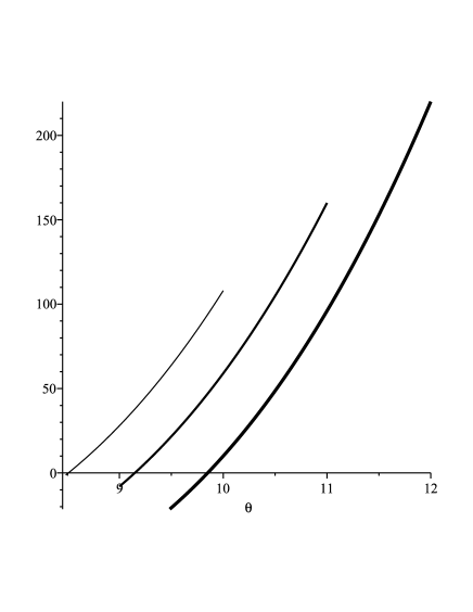
Thus we proved the assertions of (i) corresponding to the case $\theta\leq\theta_{c}=q+1$.

Case: $z_{1}<1$. Using the explicit formula (5.19) of $\sqrt{z_{1}}$ and the condition $\theta>\theta_{m}$ we get $\theta\sqrt{z_{1}}>1$. Indeed,

$$\theta\sqrt{z_{1}}>1\ \ \Leftrightarrow\ \ {2(q-m)\theta\over\theta-1+\sqrt{(\theta-1)^{2}-4m(q-m)}}>1\ \ \Leftrightarrow$$

$$(2(q-m)-1)\theta+1>\sqrt{(\theta-1)^{2}-4m(q-m)}\ \ \Leftrightarrow$$

$$(q-m-1)\theta^{2}+\theta+m>0.$$

The last inequality is true for any $\theta>1$. Consequently, using $\theta>\sqrt{z_{1}}$, $\theta\sqrt{z_{1}}>1$ and $z_{1}<1$ from formula (5.5) replacing in it $z_{1}$ by $(1/m)((\theta-1)\sqrt{z_{1}}-q+m)$, we get independently on the values of $q$ and $m$ that

$$c={1\over Z_{1}}\left(\theta\sqrt{z_{1}}-1\right).$$

For $z_{1}<1$ we have $a<b$ (see (3.24)). Now, to prove that $b>c$ for $z_{1}<1$ (i.e. for $\theta>\theta_{c}$) we note that

$$b={(\theta-1)\sqrt{z_{1}}\over Z_{1}}>c={1\over Z_{1}}\left(\theta\sqrt{z_{1}}-1\right)\ \ \Leftrightarrow$$

$$(\theta-1)\sqrt{z_{1}}>\theta\sqrt{z_{1}}-1\ \ \Leftrightarrow\ \ 1>\sqrt{z_{1}}\ \ \Leftrightarrow\ \ 1>z_{1}.$$

Consequently, $\kappa=\max\{a,b,c\}=b$ and to check $2\gamma\kappa\leq 1$ it suffices that

$${2(\theta-1)^{2}\sqrt{z_{1}}\over(\theta+1)[(\theta+m-1)z_{1}+q-m]}<1.$$ (5.23)

Again using that $z_{1}$ is a solution of $mz_{1}-(\theta-1)\sqrt{z_{1}}+q-m=0$, for $m=2$ one can simplify the inequality (5.23) to the following

$$(\theta^{2}-2\theta+5)\sqrt{z_{1}}-(q-2)(\theta+1)>0.$$

Now, from this inequality, using $\sqrt{z_{1}}=2(q-2)/[\theta-1+\sqrt{(\theta-1)^{2}-8(q-2)}]$ (see (5.19), for $m=2$) we get

$$g(\theta,q)=\theta^{3}-(q+3)\theta^{2}-(2q-15)\theta-(q+13)<0.$$

The equation

$$g^{\prime}(\theta,q)=3\theta^{2}-2(q+3)\theta-(2q-15)=0$$

has two solutions

$$\theta_{\pm}=1+{q\over 3}\pm{1\over 3}\sqrt{q^{2}+12q-36}.$$

Recall $\theta_{c}=q+1$. These solutions satisfy

$$\theta_{-}<\theta_{+}<\theta_{c}=q+1.$$

Thus $g(\theta,q)$ as a function of $\theta\in[\theta_{c},+\infty)$ is an increasing function. We have $g(\theta_{c},q)=-4q(q-2)<0$. Now for $q\geq 4$ we show that $g(\theta^{*},q)>0$, where $\theta^{*}$ is defined in (4.1): We compute

$$P(q)\equiv g(\theta^{*},q)=(3\sqrt{2}+4)q^{3}-4(5\sqrt{2}+8)q^{2}+4(15\sqrt{2}+14)q-112$$

and

$$P^{\prime}(q)=3(3\sqrt{2}+4)q^{2}-8(5\sqrt{2}+8)q+4(15\sqrt{2}+14).$$

The equation $P^{\prime}(q)=0$ has two solutions

$$q_{\pm}={2\over 3}\cdot{10\sqrt{2}+16\pm\sqrt{18+14\sqrt{2}}\over 3\sqrt{2}+4}.$$

These solutions satisfy $q_{-}<q_{+}<3$. Thus the function $P(q)$ is increasing for $q\geq 4$. Consequently,

$$P(q)\geq P(4)=16(7\sqrt{2}-9)>0.$$

This completes the proof of $g(\theta^{*},q)>0$, for any $q\geq 4$.

Consequently $g(\theta,q)=0$ has the unique solution $\breve{\theta}=\breve{\theta}(q)$ for each $q\geq 4$, such that $\theta_{c}<\breve{\theta}<\theta^{*}$. Thus $g(\theta,q)<0$ and $\mu_{1}(\theta,2)$ is extreme for $\theta\in[\theta_{c},\breve{\theta})$.

Summarizing the results for the case $z_{1}\geq 1$ and the case $z_{1}<1$ we get the desired assertions of (i).

Note that for $q=6$ we have $\theta^{*}=3(1+2\sqrt{2})\approx 11.485$ and a numerical analysis shows that $\breve{\theta}\approx 8.903$ (see Fig.11). So $\theta^{*}-\breve{\theta}\approx 2.582$.

Figure 11. The graph of the function $g(\theta,q)$, for $q=6$, given in the small interval $[8.88,8.92]$ show that the solution of $g(\breve{\theta},6)=0$ is $\breve{\theta}\approx 8.903$.

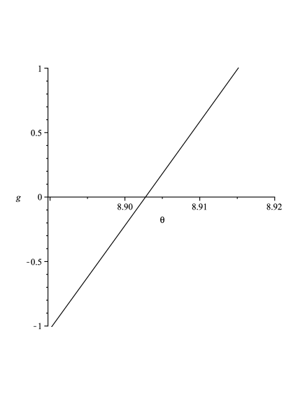
(ii) Note that $z=z_{2}>1$, for each $\theta\in[\theta_{m},+\infty)$, where $\theta_{m}=1+2\sqrt{m(q-m)}$. Recall that for $z_{2}>1$ we have $\kappa=a$ (see (5.15)). Therefore, similarly as in (5.21) we have to check

$$\theta^{2}-(2m+4)\theta-2m+3+(\theta-3)\sqrt{(\theta-1)^{2}-4m(q-m)}<0.$$ (5.24)

For $m=2$ and a given value of $q<9$, from (5.24) we obtain the assertions of (ii).

In the case $q=6$, $m=2$ it is easy to see that the LHS of (5.24) is zero for $\theta=\grave{\theta}=7$ and the inequality is true for any $\theta\in[\theta_{2},7)$. In Theorem 4.1 we proved that $\mu_{2}(\theta,m)$ is non-extreme if $\theta>\widehat{\theta}$ where $\widehat{\theta}$ is defined in (4.1) which now is $\widehat{\theta}=6\sqrt{2}-1\approx 7.4852$. So $\widehat{\theta}-7\approx 0.4852$. This is the length of the gap between the Kesten-Stigum bound of non-extremality and our bound of extremality.

(iii) For $\theta=\theta_{m}$ we have $z_{1}=z_{2}>1$ and from (5.21) we get

$$\theta_{m}^{2}-(2m+4)\theta_{m}-2m+3<0.$$ (5.25)

Using the formula $\theta_{m}=1+2\sqrt{m(q-m)}$ from (5.25) we obtain

$$q<{m+1\over 2m}\left[3m+1+\sqrt{m^{2}+6m+1}\right],\ \ m\geq 2.$$ (5.26)

This completes the proof. ∎

5.5. A continuity argument.

Let us conclude the paper with softer results which are valid for $\theta$ close to the critical value $\theta_{c}$ at which the lower branches of the boundary law $z$ degenerate into the free value $z=1$ and the corresponding Markov chains become close to the free chain.

Proof of Theorem 5.4

Proof.

a) As it was shown above $\gamma$ and $\kappa$ are bounded by continuous functions of $\theta$. For $\theta=\theta_{c}=q+1$ we have $z_{1}=1$, $a=b=c={\theta_{c}-1\over\theta_{c}-1+q}={1\over 2}$, $\gamma\leq{\theta_{c}-1\over\theta_{c}+1}={q\over q+2}$ and $\kappa=a=b=c={1\over 2}$. The measure $\mu_{0}$ (corresponding to the solution $z=(1,1,\dots,1)$) is extreme at $\theta=\theta_{c}$ if $2\gamma\kappa\leq 1$. We have

$$2\gamma\kappa\leq 2a{\theta_{c}-1\over\theta_{c}+1}={q\over q+2}<1,\ \ \mbox{for all}\ \ q\geq 2.$$

Hence $\mu_{0}$ is extreme at $\theta=\theta_{c}$. Since $\mu_{1}(\theta_{c},m)=\mu_{0}$, by the above-mentioned continuity in a sufficiently small neighborhood of $\theta_{c}$ the measure $\mu_{1}(\theta,m)$ is extreme.

b) This follows from Theorem 5.3 using the continuity similarly as in case a). ∎

Proof of Theorem 5.5

Proof.

By Proposition 2.4 we know that for $\theta_{[q/2]}<\theta\neq\theta_{c}$ there are $2^{q}-1$ TISGMs. One of them corresponds to $z=1$. Half of the remaining $2^{q}-2$, i.e. $2^{q-1}-1$, TISGMs are generated by $z_{1}$ and the other $2^{q-1}-1$ TISGMs are generated by $z_{2}$. By the above-mentioned results we know that $\mu_{2}(\theta,1)$ is extreme. The number of such measures is $q$. By Theorem 5.4, in a sufficiently small punctured neighborhood of $\theta_{c}$ all measures $\mu_{1}(\theta,m)$ are extreme. Thus the total number of extremal TISGM is at least $2^{q-1}+q$. ∎

References

- [1] C. Borgs, J. Chayes, E. Mossel, S. Roch, The Kesten-Stigum reconstruction bound is tight for roughly symmetric binary channels, FOCS, 2006, 47th Annual IEEE Conference on Foundations of Computer Science, 2006, pp. 518-530. Preprint available at arXiv:math/0604366v1.
- [2] G.R. Brightwell, P. Winkler, Graph homomorphisms and phase transitions, J. Combin. Theory Ser. B 77(2) (1999), 221–262.
- [3] A.C.D. van Enter, R. Fernández, A.D. Sokal, Regularity properties and pathologies of position-space renormalization-group transformations: Scope and limitations of Gibbsian theory, J. Stat. Phys. 72 (1993), 879–1167
- [4] A.C.D. van Enter, V. N. Ermolaev, G. Iacobelli, C. Külske, Gibbs-non-Gibbs properties for evolving Ising models on trees. Ann. Inst. Henri Poincar Probab. Stat.48(3) (2012), 774–791.
- [5] M. Formentin, C. Külske, A symmetric entropy bound on the non-reconstruction regime of Markov chains on Galton-Watson trees. Electron. Commun. Probab. 14 (2009), 587–596.
- [6] N.N. Ganikhodjaev, On pure phases of the three-state ferromagnetic Potts model on the second-order Bethe lattice. Theor. Math. Phys. 85(2) (1990), 1125–1134.
- [7] N.N. Ganikhodjaev, On pure phases of the ferromagnetic Potts model Bethe lattices, Dokl. AN Uzbekistan. No. 6-7 (1992), 4–7.
- [8] H.O. Georgii, Gibbs Measures and Phase Transitions, Second edition. de Gruyter Studies in Mathematics, 9. Walter de Gruyter, Berlin, 2011.
- [9] O. Häggström, The random-cluster model on a homogeneous tree, Probab. Theory and Relat. Fields 104 (1996) 231–253.
- [10] O. Häggström, Is the fuzzy Potts model Gibbsian? Ann. Inst. H. Poincare Probab. Statist. 39 (2003), 891–917.
- [11] B.Jahnel, C.Külske, E.Rudelli, J.Wegener, Gibbsian and non-Gibbsian properties of the generalized mean-field fuzzy Potts model. Markov Processes and Related Fields, 20 (2014) 601–632.
- [12] H. Kesten, B.P. Stigum, Additional limit theorem for indecomposable multi-dimensional Galton-Watson processes, Ann. Math. Statist. 37 (1966), 1463–1481.
- [13] O. Häggström, C. Külske, Gibbs properties of the fuzzy Potts model on trees and in mean field, Markov Proc. Rel. Fields 10(3) (2004), 477–506.
- [14] C. Külske, U.A. Rozikov, R.M. Khakimov, Description of the translation-invariant splitting Gibbs measures for the Potts model on a Cayley tree, Jour. Stat. Phys. 156(1) (2014), 189-200.
- [15] C. Külske, Regularity properties of potentials for joint measures of random spin systems, Markov Proc.Rel.Fields 10 (1) (2004) 75–88.
- [16] C. Maes, V.K. Vande, The fuzzy Potts model. J. Phys. A 28(15) (1995), 4261–4270.
- [17] J.B. Martin, Reconstruction thresholds on regular trees. Discrete random walks (Paris, 2003), 191–204 (electronic), Discrete Math. Theor. Comput. Sci. Proc., AC, Assoc. Discrete Math. Theor. Comput. Sci., Nancy, 2003.
- [18] F. Martinelli, A. Sinclair, D. Weitz, Fast mixing for independent sets, coloring and other models on trees. Random Structures and Algoritms, 31 (2007), 134-172.
- [19] M. Mézard, A. Montanari, Reconstruction on trees and spin glass transition. J. Stat. Phys. 124 (2006), 1317–1350.
- [20] E. Mossel, Y. Peres, Information flow on trees, Ann. Appl. Probab. 13(3) (2003), 817–844.
- [21] E. Mossel, Survey: Information flow on trees. Graphs, morphisms and statistical physics, 155–170, DIMACS Ser. Discrete Math. Theoret. Comput. Sci., 63, Amer. Math. Soc., Providence, RI, 2004.
- [22] E. Mossel, Reconstruction on trees: Beating the second eigenvalue, Annals Appl. Probab. 11(1) (2001), 285–300.
- [23] V.V. Prasolov, Polynomials (Springer-Verlag Berlin Heidelberg, 2004)
- [24] U.A. Rozikov, Gibbs measures on Cayley trees. World Sci. Publ. Singapore. 2013.
- [25] A. Sly, Reconstruction for the Potts model. Ann. Probab. 39 (2011), 1365–1406.