Models with Hidden Regular Variation:
generation and detection

Bikramjit Das Bikramjit Das
ESD
Singapore University of Technology and Design, Singapore
bikram@sutd.edu.sg
 and  Sidney I. Resnick Sidney I. Resnick
School of ORIE, Cornell University, Ithaca, NY 14853 USA
sir1@cornell.edu
Abstract.

We review definitions of multivariate regular variation (MRV) and hidden regular variation (HRV) for distributions of random vectors and then summarize methods for generating models exhibiting both properties. We also discuss diagnostic techniques that detect these properties in multivariate data and indicate when models exhibiting both MRV and HRV are plausible fits for the data. We illustrate our techniques on simulated data and also two real Internet data sets.

Key words and phrases:
regular variation, multivariate heavy tails, hidden regular variation, tail estimation, conditional extreme value model
2010 Mathematics Subject Classification:
28A33,60G17,60G51,60G70
B. Das was supported by SRG-ESD-2012-047. S. Resnick was supported by Army MURI grant W911NF-12-1-0385 to Cornell University. Resnick acknowledges hospitality, space and support from SUTD during a visit January 2014.

1. Introduction

Data exhibiting heavy tails appear naturally in many contexts, for example hydrology [1], finance [26], insurance [11], Internet traffic and telecommunication [4] and risk assessment [7, 16]. Often the observed data are multi-dimensional with heavy tailed marginal distributions and come from complex systems and we must study the dependence structure among the components.

The study of multivariate heavy-tailed models is facilitated by the ability to generate such models. Moreover, a generation technique helps in stress-testing worst-case scenarios. In the first part of this paper we consider several generation techniques and discuss their strengths and weaknesses.

A second theme of this paper is the development of diagnostics for detecting and identifying multivariate heavy tailed models prior to estimating model parameters. The second part of this paper deals with this.

1.1. Outline

The mathematical framework for the study of multivariate heavy tails is regular variation of measures. We provide a careful review of the definitions of multivariate regular variation (MRV) and hidden regular variation (HRV) in Section 1.2 and list the notations we use in Section 1.3. In Section 2 we discuss methods for generating regularly varying models on 𝔼=[0,)2{(0,0)}𝔼superscript0200\mathbb{E}=[0,\infty)^{2}\smallsetminus\{(0,0)\} and 𝔼0=(0,)2subscript𝔼0superscript02\mathbb{E}_{0}=(0,\infty)^{2} when the asymptotic limit measures are specified. The described methods are relatively easy to implement.

In Section 3 we discuss how to create models that exhibit both MRV and HRV. Both MRV and HRV are asymptotic models with curious properties which are often ignored or misinterpreted when attempting to generate finite samples exhibiting such properties. We review three model generation methods that yield the asymptotic properties of both MRV on 𝔼𝔼\mathbb{E} and HRV on 𝔼0subscript𝔼0\mathbb{E}_{0} and discuss characteristics of each method. These methods are called (i) the mixture method, (ii) the multiplication method and (iii) the additive method. We give particular attention to the recently proposed additive generation method of [27] and show that there are identifiability issues in the sense that asymptotic parameters may not be coming from the anticipated summand of the representation. Accompanying simulation examples illustrate our discussion.

Section 4 gives techniques for detecting when data is consistent with a model exhibiting MRV and HRV. These techniques rely on the fact that under broad conditions, if a vector 𝑿𝑿\boldsymbol{X} has a multivariate regularly varying distribution on a cone \mathbb{C}, then under a generalized polar coordinate transformation (see (1.4)), the transformed vector satisfies a conditional extreme value (CEV) model for which detection techniques exist from [6]. This methodology goes beyond one dimensional techniques such as checking one dimensional marginal distributions are heavy tailed or checking one dimensional functions of the data vector such as maximum and minimum component are heavy tailed.

In Section 5, we give two examples of our detection and model estimation techniques applied to Internet downloads and HTTP response data.

1.2. Regularly varying distributions on cones.

We review material from [15, 8, 18] describing the framework for the definition of MRV and HRV and then specialize to two dimensions.

Let 𝕏𝕏\mathbb{X} be a metric space with metric d(𝒙,𝒚)𝑑𝒙𝒚d(\boldsymbol{x},\boldsymbol{y}) satisfying

(1.1) d(c𝒙,c𝒚)=cd(𝒙,𝒚),c>0,(𝒙,𝒚)𝕏×𝕏.formulae-sequence𝑑𝑐𝒙𝑐𝒚𝑐𝑑𝒙𝒚formulae-sequence𝑐0𝒙𝒚𝕏𝕏d(c\boldsymbol{x},c\boldsymbol{y})=cd(\boldsymbol{x},\boldsymbol{y}),\qquad c>0,(\boldsymbol{x},\boldsymbol{y})\in\mathbb{X}\times\mathbb{X}.

If d(,)𝑑d(\cdot,\cdot) is defined by a norm, (1.1) is satisfied. Hence in finite dimensional Euclidean space, (1.1) can always be satisfied. A flexible framework for discussing regular variation is measure convergence defined by 𝕄𝕄\mathbb{M}-convergence [18, 8]) on a closed cone 𝕏𝕏\mathbb{C}\subset\mathbb{X} with a closed cone 0subscript0\mathbb{C}_{0}\subset\mathbb{C} deleted. The concept of a cone requires specifying a definition of scalar multiplication (c,𝒙)c𝒙maps-to𝑐𝒙𝑐𝒙(c,\boldsymbol{x})\mapsto c\boldsymbol{x} from +×𝕏𝕏maps-tosubscript𝕏𝕏\mathbb{R}_{+}\times\mathbb{X}\mapsto\mathbb{X}. In this paper, the metric space is Euclidean and scalar multiplication is the usual one. A cone \mathbb{C} is closed under scalar multiplication: If 𝒙𝒙\boldsymbol{x}\in\mathbb{C} then c𝒙𝑐𝒙c\boldsymbol{x}\in\mathbb{C} for c>0𝑐0c>0. A subset Λ0Λsubscript0\Lambda\subset\mathbb{C}\smallsetminus\mathbb{C}_{0} is bounded away from 0subscript0\mathbb{C}_{0} if d(Λ,0)>0𝑑Λsubscript00d(\Lambda,\mathbb{C}_{0})>0. The two cases of most interest are

  1. (1)

    =+2superscriptsubscript2\mathbb{C}=\mathbb{R}_{+}^{2} and 0={𝟎}subscript00\mathbb{C}_{0}=\{\boldsymbol{0}\}. Then 𝔼:=0=+2{𝟎}assign𝔼subscript0superscriptsubscript20\mathbb{E}:=\mathbb{C}\smallsetminus\mathbb{C}_{0}=\mathbb{R}_{+}^{2}\smallsetminus\{\boldsymbol{0}\} is the space for defining 𝕄𝕄\mathbb{M}-convergence appropriate for regular variation of distributions of positive random vectors.

  2. (2)

    =+2superscriptsubscript2\mathbb{C}=\mathbb{R}_{+}^{2} and 0={𝒙:i=12xi=0}:=[axes]subscript0conditional-set𝒙superscriptsubscript𝑖12subscript𝑥𝑖0assigndelimited-[]axes\mathbb{C}_{0}=\{\boldsymbol{x}:\wedge_{i=1}^{2}x_{i}=0\}:=[\text{axes}]. Then 𝔼0:=0assignsubscript𝔼0subscript0\mathbb{E}_{0}:=\mathbb{C}\smallsetminus\mathbb{C}_{0}, the first quadrant without its axes, is the space for defining 𝕄𝕄\mathbb{M}-convergence appropriate for HRV.

A random vector 𝒁𝟎𝒁0\boldsymbol{Z}\geqslant\boldsymbol{0} is regularly varying on 0subscript0\mathbb{C}\smallsetminus\mathbb{C}_{0} if there exists a regularly varying function b(t)RV1/α𝑏𝑡𝑅subscript𝑉1𝛼b(t)\in RV_{1/\alpha}, α>0𝛼0\alpha>0 called the scaling function and a measure ν()𝕄(0)𝜈𝕄subscript0\nu(\cdot)\in\mathbb{M}(\mathbb{C}\smallsetminus\mathbb{C}_{0}) called the limit or tail measure such that as t𝑡t\to\infty,

(1.2) t𝐏[𝒁/b(t)]ν(),𝑡𝐏delimited-[]𝒁𝑏𝑡𝜈t\mathbf{P}[\boldsymbol{Z}/b(t)\in\cdot\,]\to\nu(\cdot),

in 𝕄(0)𝕄subscript0\mathbb{M}(\mathbb{C}\smallsetminus\mathbb{C}_{0}), the set of measures on 0subscript0\mathbb{C}\smallsetminus\mathbb{C}_{0} which are finite on sets bounded away from 0subscript0\mathbb{C}_{0} [8, 15, 18]. We write 𝒁MRV(α,b(t),ν,0)𝒁𝑀𝑅𝑉𝛼𝑏𝑡𝜈subscript0\boldsymbol{Z}\in MRV(\alpha,b(t),\nu,\mathbb{C}\smallsetminus\mathbb{C}_{0}). Since b(t)RV1/α𝑏𝑡𝑅subscript𝑉1𝛼b(t)\in RV_{1/\alpha}, ν()𝜈\nu(\cdot) has a scaling property

(1.3) ν(c)=cαν(),c>0.\nu(c\cdot)=c^{-\alpha}\nu(\cdot),\qquad c>0.

When =+2superscriptsubscript2\mathbb{C}=\mathbb{R}_{+}^{2}, 0={𝟎}subscript00\mathbb{C}_{0}=\{\boldsymbol{0}\} and ν𝜈\nu satisfies ν(𝒙,)=0𝜈𝒙0\nu(\boldsymbol{x},\boldsymbol{\infty})=0 for all 𝒙>𝟎𝒙0\boldsymbol{x}>\boldsymbol{0} so that ν𝜈\nu concentrates on the axes, we say 𝒁𝒁\boldsymbol{Z} possesses asymptotic independence [23, 9, 24]. It is convenient to translate (1.2) and (1.3) using generalized polar coordinates [18, 8]. Set 0={𝒙0:d(𝒙,0)=1},subscriptsubscript0conditional-set𝒙subscript0𝑑𝒙subscript01\aleph_{\mathbb{C}_{0}}=\{\boldsymbol{x}\in\mathbb{C}\smallsetminus\mathbb{C}_{0}:d(\boldsymbol{x},\mathbb{C}_{0})=1\}, the locus of points at distance 1 from the deleted region 0subscript0\mathbb{C}_{0}. Define GPOLAR:0(0,)×0:GPOLARmaps-tosubscript00subscriptsubscript0\text{GPOLAR}:\mathbb{C}\smallsetminus\mathbb{C}_{0}\mapsto(0,\infty)\times\aleph_{\mathbb{C}_{0}} by

(1.4) GPOLAR(𝒙)=(d(𝒙,0),𝒙d(𝒙,0))GPOLAR𝒙𝑑𝒙subscript0𝒙𝑑𝒙subscript0\text{GPOLAR}(\boldsymbol{x})=\Bigl{(}d(\boldsymbol{x},\mathbb{C}_{0}),\frac{\boldsymbol{x}}{d(\boldsymbol{x},\mathbb{C}_{0})}\Bigr{)}

Then ([8, 18]) (1.2) and (1.3) are equivalent to

(1.5) t𝐏[GPOLAR(𝒁)/b(t)]να×S()=νGPOLAR1,𝑡𝐏delimited-[]GPOLAR𝒁𝑏𝑡subscript𝜈𝛼𝑆𝜈superscriptGPOLAR1t\mathbf{P}[\text{GPOLAR}(\boldsymbol{Z})/b(t)\in\cdot\,]\to\nu_{\alpha}\times S(\cdot){=\nu\circ\text{GPOLAR}^{-1}},

in 𝕄((0,)×0)𝕄0subscriptsubscript0\mathbb{M}\bigl{(}(0,\infty)\times\aleph_{\mathbb{C}_{0}}\bigr{)} where να(x,)=xα,x>0,α>0formulae-sequencesubscript𝜈𝛼𝑥superscript𝑥𝛼formulae-sequence𝑥0𝛼0\nu_{\alpha}(x,\infty)=x^{-\alpha},\,x>0,\,\alpha>0 and S()𝑆S(\cdot) is a probability measure on 0subscriptsubscript0\aleph_{\mathbb{C}_{0}}. One should note that the transformation GPOLAR depends on the cone 0subscript0\mathbb{C}_{0}; this dependence should be understood from the context.

We focus on regular variation for p=2𝑝2p=2 and the two choices of \mathbb{C} and 0subscript0\mathbb{C}_{0} which yield the spaces

  1. (1)

    𝔼:=+2{𝟎}assign𝔼superscriptsubscript20\mathbb{E}:=\mathbb{R}_{+}^{2}\smallsetminus\{\boldsymbol{0}\}.

  2. (2)

    𝔼0=+2{𝒙:x1x2=0}=:+2[axes].\mathbb{E}_{0}=\mathbb{R}_{+}^{2}\smallsetminus\{\boldsymbol{x}:x_{1}\wedge x_{2}=0\}=:\mathbb{R}_{+}^{2}\smallsetminus[\text{axes}].

Then 𝒁𝒁\boldsymbol{Z} is regularly varying on 𝔼𝔼\mathbb{E} and has hidden regular variation (HRV) on 𝔼0subscript𝔼0\mathbb{E}_{0} if there exist 0<αα00𝛼subscript𝛼00<\alpha\leqslant\alpha_{0}, scaling functions b(t)RV1/α𝑏𝑡𝑅subscript𝑉1𝛼b(t)\in RV_{1/\alpha} and b0RV1/α0subscript𝑏0𝑅subscript𝑉1subscript𝛼0b_{0}\in RV_{1/\alpha_{0}} with b(t)/b0(t)𝑏𝑡subscript𝑏0𝑡b(t)/b_{0}(t)\to\infty and limit measures ν,ν0𝜈subscript𝜈0\nu,\,\nu_{0} such that

𝒁MRV(α,b(t),ν,𝔼)MRV(α0,b0(t),ν0,𝔼0)𝒁MRV𝛼𝑏𝑡𝜈𝔼MRVsubscript𝛼0subscript𝑏0𝑡subscript𝜈0subscript𝔼0\boldsymbol{Z}\in\text{MRV}(\alpha,b(t),\nu,\mathbb{E})\cap\text{MRV}(\alpha_{0},b_{0}(t),\nu_{0},\mathbb{E}_{0})

so that unpacking the notation we get,

(1.6) t𝐏[𝒁/b(t)]ν(), in 𝕄(𝔼)𝑡𝐏delimited-[]𝒁𝑏𝑡𝜈 in 𝕄𝔼t\mathbf{P}[\boldsymbol{Z}/b(t)\in\cdot\,]\to\nu(\cdot),\quad\text{ in }\mathbb{M}(\mathbb{E})

and

(1.7) t𝐏[𝒁/b0(t)]ν0(), in 𝕄(𝔼0).𝑡𝐏delimited-[]𝒁subscript𝑏0𝑡subscript𝜈0 in 𝕄subscript𝔼0t\mathbf{P}[\boldsymbol{Z}/b_{0}(t)\in\cdot\,]\to\nu_{0}(\cdot),\quad\text{ in }\mathbb{M}(\mathbb{E}_{0}).

On 𝔼𝔼\mathbb{E} we may take 𝟎={𝒙:𝒙=1}subscript0conditional-set𝒙norm𝒙1\aleph_{\boldsymbol{0}}=\{\boldsymbol{x}:\|\boldsymbol{x}\|=1\} for a convenient choice of d(𝒙,𝒚)=𝒙𝒚𝑑𝒙𝒚norm𝒙𝒚d(\boldsymbol{x},\boldsymbol{y})=\|\boldsymbol{x}-\boldsymbol{y}\| and on 𝔼0subscript𝔼0\mathbb{E}_{0},

[axes]:={𝒙𝔼:x1x2=1}assignsubscriptdelimited-[]axesconditional-set𝒙𝔼subscript𝑥1subscript𝑥21\aleph_{[\text{axes}]}:=\{\boldsymbol{x}\in\mathbb{E}:x_{1}\wedge x_{2}=1\}

is the appropriate unit sphere. Then using GPOLAR (1.6) and (1.7) become,

(1.8) t𝐏[(𝒁/b(t),𝒁/𝒁)]να×S(), in 𝕄((0,)×𝟎)𝑡𝐏delimited-[]norm𝒁𝑏𝑡𝒁norm𝒁subscript𝜈𝛼𝑆 in 𝕄0subscript0t\mathbf{P}\bigl{[}\bigl{(}\|\boldsymbol{Z}\|/b(t),\boldsymbol{Z}/\|\boldsymbol{Z}\|\bigr{)}\in\cdot\,\bigr{]}\to\nu_{\alpha}\times S(\cdot),\quad\text{ in }\mathbb{M}((0,\infty)\times\aleph_{\boldsymbol{0}})

and

(1.9) t𝐏[(Z1Z2b0(t),𝒁Z1Z2)]να0×S0() in 𝕄((0,)×[axes])𝑡𝐏delimited-[]subscript𝑍1subscript𝑍2subscript𝑏0𝑡𝒁subscript𝑍1subscript𝑍2subscript𝜈subscript𝛼0subscript𝑆0 in 𝕄0subscriptdelimited-[]axest\mathbf{P}\Bigl{[}\Bigl{(}\frac{Z_{1}\wedge Z_{2}}{b_{0}(t)},\frac{\boldsymbol{Z}}{Z_{1}\wedge Z_{2}}\Bigr{)}\in\cdot\Bigr{]}\to\nu_{\alpha_{0}}\times S_{0}(\cdot)\qquad\text{ in }\mathbb{M}\bigl{(}(0,\infty)\times\aleph_{[\text{axes}]}\bigr{)}

and S𝑆S and S0subscript𝑆0S_{0} are probability measures on 𝟎subscript0\aleph_{\boldsymbol{0}} and [axes]subscriptdelimited-[]axes\aleph_{[\text{axes}]} respectively. Note

(𝒛z1z2)={(1,z2/z1), if z1z2,(z1/z2,1), if z2<z1𝒛subscript𝑧1subscript𝑧2cases1subscript𝑧2subscript𝑧1 if subscript𝑧1subscript𝑧2subscript𝑧1subscript𝑧21 if subscript𝑧2subscript𝑧1\Bigl{(}\frac{\boldsymbol{z}}{z_{1}\wedge z_{2}}\Bigr{)}=\begin{cases}(1,z_{2}/z_{1}),&\text{ if }z_{1}\leqslant z_{2},\\ (z_{1}/z_{2},1),&\text{ if }z_{2}<z_{1}\end{cases}

and

[axes]=([1,)×{1})({1}×[1,)).subscriptdelimited-[]axes1111\aleph_{[\text{axes}]}=\bigl{(}[1,\infty)\times\{1\}\bigr{)}\cup\bigl{(}\{1\}\times[1,\infty)\bigr{)}.

So we may rewrite (1.9) as two statements: For x1𝑥1x\geqslant 1,

(1.10) t𝐏[Z1b0(t)>r,Z2Z1>x]rα0S0{(1,z):z>x}=:rα0pG¯1(x),\displaystyle t\mathbf{P}[\frac{Z_{1}}{b_{0}(t)}>r,\frac{Z_{2}}{Z_{1}}>x]\to r^{-\alpha_{0}}S_{0}\{(1,z):z>x\}=:r^{-\alpha_{0}}p\bar{G}_{1}(x),
(1.11) t𝐏[Z2b0(t)>r,Z1Z2>x]rα0S0{(z,1):z>x}=:rα0qG¯2(x),\displaystyle t\mathbf{P}[\frac{Z_{2}}{b_{0}(t)}>r,\frac{Z_{1}}{Z_{2}}>x]\to r^{-\alpha_{0}}S_{0}\{(z,1):z>x\}=:r^{-\alpha_{0}}q\bar{G}_{2}(x),

where p:=S0{{1}×[1,)},assign𝑝subscript𝑆011p:=S_{0}\{\{1\}\times[1,\infty)\}, q:=S0{[1,)×{1}}=1passign𝑞subscript𝑆0111𝑝q:=S_{0}\{[1,\infty)\times\{1\}\}=1-p and G1,G2subscript𝐺1subscript𝐺2G_{1},G_{2} are probability distributions on [1,)1[1,\infty). We also have

(1.12) t𝐏[Z1Z2b0(t)>r,(Z1Z2Z2Z1)>x]rα0(pG¯1(x)+qG¯2(x)).𝑡𝐏delimited-[]formulae-sequencesubscript𝑍1subscript𝑍2subscript𝑏0𝑡𝑟subscript𝑍1subscript𝑍2subscript𝑍2subscript𝑍1𝑥superscript𝑟subscript𝛼0𝑝subscript¯𝐺1𝑥𝑞subscript¯𝐺2𝑥\displaystyle t\mathbf{P}[\frac{Z_{1}\wedge Z_{2}}{b_{0}(t)}>r,\left(\frac{Z_{1}}{Z_{2}}\bigvee\frac{Z_{2}}{Z_{1}}\right)>x]\to r^{-\alpha_{0}}\left(p\bar{G}_{1}(x)+q\bar{G}_{2}(x)\right).

Traditionally [23], regular variation on 𝔼𝔼\mathbb{E} has been studied using the one point uncompactification, vague convergence and the polar coordinate transform 𝒙(𝒙,𝒙/𝒙).maps-to𝒙norm𝒙𝒙norm𝒙\boldsymbol{x}\mapsto(\|\boldsymbol{x}\|,\boldsymbol{x}/\|\boldsymbol{x}\|). On 𝔼𝔼\mathbb{E} this works fine because {𝒙𝔼:𝒙=1}conditional-set𝒙𝔼norm𝒙1\{\boldsymbol{x}\in\mathbb{E}:\|\boldsymbol{x}\|=1\} is compact and lines through \boldsymbol{\infty} cannot carry mass. However, on 𝔼0subscript𝔼0\mathbb{E}_{0} the traditional unit sphere {𝒙𝔼0:𝒙=1}conditional-set𝒙subscript𝔼0norm𝒙1\{\boldsymbol{x}\in\mathbb{E}_{0}:\|\boldsymbol{x}\|=1\} is no longer compact. Hence, Radon measures on {𝒙𝔼0:𝒙=1}conditional-set𝒙subscript𝔼0norm𝒙1\{\boldsymbol{x}\in\mathbb{E}_{0}:\|\boldsymbol{x}\|=1\} may not be finite and for estimation problems the approach relying on vague convergence is a dead end if estimation of a possibly infinite measure is required. More details on why an approach without compactification is desirable are in [15, 8, 18]. We emphasize it is difficult to discuss MRV on 𝔼0subscript𝔼0\mathbb{E}_{0} with the conventional unit sphere and it is preferable to use [axes]subscriptdelimited-[]axes\aleph_{[\text{axes}]}.

1.3. Basic notation

Here is a notation and concept summary.

RVβRegularly varying functions with index β>0. We can and doassume such functions are continuous and strictly increasing.𝔼2{𝟎}.[axes]{0}×++×{0}.𝔼02[axes].𝕄(0)The set of all non-zero measures on 0 which are finite on subsets bounded away from 0.𝒞(0)Continuous, bounded, positive functions on 0 whose supportsare bounded away from 0. Without loss of generality [18], we mayassume the functions are uniformly continuous.μnμConvergence in 𝕄(0) means μn(f)μ(f) for allf𝒞(0). See [15, 8, 18].{𝒙:d(𝒙,)=1}.𝟎{𝒙𝔼:d(𝒙,{𝟎})=1}.[axes]{𝒙𝔼0:d(𝒙,[axes])=1}={1}×[1,)[1,)×{1}.MRVmultivariate regular variation; for this paper, it means regular variation on 𝔼.HRVhidden regular variation; for this paper, it means regular variation on 𝔼0.GPOLARPolar co-ordinate transformation relative to the deleted cone 0,GPOLAR(𝒙)=(d(𝒙,0),𝒙/d(𝒙,0)). See [18, 8].𝑿𝒀The random elements 𝑿,𝒀 are independent.𝑅subscript𝑉𝛽Regularly varying functions with index β>0. We can and domissing-subexpressionmissing-subexpressionmissing-subexpressionassume such functions are continuous and strictly increasing.missing-subexpressionmissing-subexpression𝔼superscript20missing-subexpressionmissing-subexpressiondelimited-[]axes0subscriptsubscript0missing-subexpressionmissing-subexpressionsubscript𝔼0superscript2delimited-[]axesmissing-subexpressionmissing-subexpression𝕄subscript0The set of all non-zero measures on 0 which are finite onmissing-subexpressionmissing-subexpressionmissing-subexpression subsets bounded away from 0.missing-subexpressionmissing-subexpression𝒞subscript0Continuous, bounded, positive functions on 0 whose supportsmissing-subexpressionmissing-subexpressionmissing-subexpressionare bounded away from 0. Without loss of generality [18], we maymissing-subexpressionmissing-subexpressionmissing-subexpressionassume the functions are uniformly continuous.missing-subexpressionmissing-subexpressionsubscript𝜇𝑛𝜇Convergence in 𝕄(0) means μn(f)μ(f) for allmissing-subexpressionmissing-subexpressionmissing-subexpressionformulae-sequence𝑓𝒞subscript0 See [15, 8, 18].missing-subexpressionmissing-subexpressionsubscriptconditional-set𝒙𝑑𝒙1missing-subexpressionmissing-subexpressionsubscript0conditional-set𝒙𝔼𝑑𝒙01missing-subexpressionmissing-subexpressionsubscriptdelimited-[]axesconditional-set𝒙subscript𝔼0𝑑𝒙delimited-[]axes11111missing-subexpressionmissing-subexpressionMRVmultivariate regular variation; for this paper, it means regular variation on 𝔼missing-subexpressionmissing-subexpressionHRVhidden regular variation; for this paper, it means regular variation on 𝔼0missing-subexpressionmissing-subexpressionGPOLARPolar co-ordinate transformation relative to the deleted cone 0,missing-subexpressionmissing-subexpressionmissing-subexpressionformulae-sequenceGPOLAR𝒙𝑑𝒙subscript0𝒙𝑑𝒙subscript0 See [18, 8].missing-subexpressionmissing-subexpressionperpendicular-toabsentperpendicular-to𝑿𝒀The random elements 𝑿,𝒀 are independent.missing-subexpressionmissing-subexpression\begin{array}[]{llll}RV_{\beta}&\text{Regularly varying functions with index $\beta>0$. We can and do}\\ &\text{assume such functions are continuous and strictly increasing.}\\[5.69054pt] \mathbb{E}&\mathbb{R}^{2}\smallsetminus\{\boldsymbol{0}\}.\\[5.69054pt] [\text{axes}]&\{0\}\times\mathbb{R}_{+}\cup\mathbb{R}_{+}\times\{0\}.\\[5.69054pt] \mathbb{E}_{0}&\mathbb{R}^{2}\smallsetminus[\text{axes}].\\[5.69054pt] \mathbb{M}(\mathbb{C}\smallsetminus\mathbb{C}_{0})&\text{The set of all non-zero measures on $\mathbb{C}\smallsetminus\mathbb{C}_{0}$ which are finite on}\\ &\text{ subsets bounded away from $\mathbb{C}_{0}$.}\\[5.69054pt] \mathcal{C}(\mathbb{C}\smallsetminus\mathbb{C}_{0})&\text{Continuous, bounded, positive functions on $\mathbb{C}\smallsetminus\mathbb{C}_{0}$ whose supports}\\ &\text{are bounded away from $\mathbb{C}_{0}$. Without loss of generality \cite[citep]{[\@@bibref{Number}{lindskog:resnick:roy:2013}{}{}]}, we may}\\ &\text{assume the functions are uniformly continuous.}\\[5.69054pt] \mu_{n}\to\mu&\text{Convergence in $\mathbb{M}(\mathbb{C}\smallsetminus\mathbb{C}_{0})$ means $\mu_{n}(f)\to\mu(f)$ for all}\\ &f\in\mathcal{C}(\mathbb{C}\smallsetminus\mathbb{C}_{0}).\text{ See \cite[cite]{[\@@bibref{Number}{hult:lindskog:2006a, das:mitra:resnick:2013, lindskog:resnick:roy:2013}{}{}]}.}\\[5.69054pt] \aleph_{\mathbb{C}}&\{\boldsymbol{x}:d(\boldsymbol{x},\mathbb{C})=1\}.\\[5.69054pt] \aleph_{\boldsymbol{0}}&\{\boldsymbol{x}\in\mathbb{E}:d(\boldsymbol{x},\{\boldsymbol{0}\})=1\}.\\[5.69054pt] \aleph_{[\text{axes}]}&\{\boldsymbol{x}\in\mathbb{E}_{0}:d(\boldsymbol{x},[\text{axes}])=1\}=\{1\}\times[1,\infty)\cup[1,\infty)\times\{1\}.\\[5.69054pt] \text{MRV}&\text{multivariate regular variation; for this paper, it means regular variation on $\mathbb{E}$}.\\[5.69054pt] \text{HRV}&\text{hidden regular variation; for this paper, it means regular variation on $\mathbb{E}_{0}$}.\\[5.69054pt] \text{GPOLAR}&\text{{Polar co-ordinate transformation} relative to the deleted cone $\mathbb{C}_{0}$,}\\ &\text{GPOLAR}(\boldsymbol{x})=\bigl{(}d(\boldsymbol{x},\mathbb{C}_{0}),\boldsymbol{x}/d(\boldsymbol{x},\mathbb{C}_{0})\bigr{)}.\text{ See \cite[cite]{[\@@bibref{Number}{lindskog:resnick:roy:2013, das:mitra:resnick:2013}{}{}]}.}\\[5.69054pt] \boldsymbol{X}\mathchoice{\mathrel{\hbox to0.0pt{$\displaystyle\perp$\hss}\mkern 2.0mu{\displaystyle\perp}}}{\mathrel{\hbox to0.0pt{$\textstyle\perp$\hss}\mkern 2.0mu{\textstyle\perp}}}{\mathrel{\hbox to0.0pt{$\scriptstyle\perp$\hss}\mkern 2.0mu{\scriptstyle\perp}}}{\mathrel{\hbox to0.0pt{$\scriptscriptstyle\perp$\hss}\mkern 2.0mu{\scriptscriptstyle\perp}}}\boldsymbol{Y}&\text{The random elements $\boldsymbol{X},\boldsymbol{Y}$ are independent.}\end{array}

2. Generating Regularly Varying Models

We outline schemes for generating regular variation. These schemes generate the full totality of asymptotic limits but not the full totality of pre-asymptotic models; so there can be many other ways to get the same asymptotic models.

2.1. Generating regular variation on 𝔼𝔼\mathbb{E}.

The easiest way to obtain a regularly varying model on 𝔼𝔼\mathbb{E} with scaling function b(t)𝑏𝑡b(t) and limit measure ν()=να×SGPOLAR𝜈subscript𝜈𝛼𝑆GPOLAR\nu(\cdot)=\nu_{\alpha}\times S\circ{\text{GPOLAR}} is as follows: Suppose R𝑅R is a random element of (0,)0(0,\infty) with a regularly varying tail and scaling function b(t)𝑏𝑡b(t):

t𝐏[R/b(t)>x]xα,x>0,α>0.formulae-sequence𝑡𝐏delimited-[]𝑅𝑏𝑡𝑥superscript𝑥𝛼formulae-sequence𝑥0𝛼0t\mathbf{P}[R/b(t)>x]\to x^{-\alpha},\quad x>0,\,\alpha>0.

Let 𝚯𝚯\boldsymbol{\Theta} be a random element of 𝟎subscript0\aleph_{\boldsymbol{0}} with distribution S𝑆S

𝐏[𝚯]=S()𝐏delimited-[]𝚯𝑆\mathbf{P}[\boldsymbol{\Theta}\in\cdot\,]=S(\cdot)

and which is independent of R𝑅R. Then 𝒁:=R𝚯=GPOLAR(R,𝚯)assign𝒁𝑅𝚯superscriptGPOLAR𝑅𝚯\boldsymbol{Z}:=R\boldsymbol{\Theta}=\text{GPOLAR}^{\leftarrow}(R,\boldsymbol{\Theta}) is regularly varying on 𝔼𝔼\mathbb{E} with limit measure ν=να×SGPOLAR𝜈subscript𝜈𝛼𝑆GPOLAR\nu=\nu_{\alpha}\times S\circ{\text{GPOLAR}} on 𝔼𝔼\mathbb{E} because (1.8) and consequently (1.6) hold. Note GPOLAR is defined relative to the deleted cone {𝟎}0\{\boldsymbol{0}\}.

2.2. Generating regular variation on 𝔼0subscript𝔼0\mathbb{E}_{0} (and sometimes also on 𝔼𝔼\mathbb{E}).

As suggested in [19], we may follow the same scheme as in Section 2.1. Let R0subscript𝑅0R_{0} be a random element of (0,)0(0,\infty) that is regularly varying with index α0subscript𝛼0\alpha_{0} and scaling function b0(t)subscript𝑏0𝑡b_{0}(t). Let 𝚯0subscript𝚯0\boldsymbol{\Theta}_{0} be a random element of [axes]subscriptdelimited-[]axes\aleph_{[\text{axes}]} with distribution S0subscript𝑆0S_{0} and independent of R0subscript𝑅0R_{0}. Then 𝒁=R0𝚯0=GPOLAR(R0,𝚯0)𝒁subscript𝑅0subscript𝚯0superscriptGPOLARsubscript𝑅0subscript𝚯0\boldsymbol{Z}=R_{0}\boldsymbol{\Theta}_{0}=\text{GPOLAR}^{\leftarrow}(R_{0},\boldsymbol{\Theta}_{0}) is regularly varying with scaling function b0(t)subscript𝑏0𝑡b_{0}(t) and limit measure ν0:=να0×S0GPOLAR1assignsubscript𝜈0subscript𝜈subscript𝛼0subscript𝑆0superscriptGPOLAR1\nu_{0}:=\nu_{\alpha_{0}}\times S_{0}\circ\text{GPOLAR}^{-1} on 𝔼0subscript𝔼0\mathbb{E}_{0} because (1.9) and therefore (1.7) hold.

In practice we specify the measure S0subscript𝑆0S_{0} on [axes]subscriptdelimited-[]axes\aleph_{[\text{axes}]} as follows: Let G1,G2subscript𝐺1subscript𝐺2G_{1},G_{2} be two probability measures on (1,)1(1,\infty) and define

(2.1) 𝚯0=B(Θ1,1)+(1B)(1,Θ2)subscript𝚯0𝐵subscriptΘ111𝐵1subscriptΘ2\boldsymbol{\Theta}_{0}=B(\Theta_{1},1)+(1-B)(1,\Theta_{2})

where B,Θ1,Θ2𝐵subscriptΘ1subscriptΘ2B,\Theta_{1},\Theta_{2} are independent, B𝐵B is a Bernoulli switching variable with P[B=1]=p=1P[B=0]𝑃delimited-[]𝐵1𝑝1𝑃delimited-[]𝐵0P[B=1]=p=1-P[B=0] and ΘisubscriptΘ𝑖\Theta_{i} has distribution Gisubscript𝐺𝑖G_{i}, i=1,2𝑖12i=1,2. So G1subscript𝐺1G_{1} smears probability mass on the horizontal line emanating from (1,1)11(1,1) and G2subscript𝐺2G_{2} does the same thing for the vertical line.

For estimation purposes, note for s>1𝑠1s>1 that

(2.2) G¯1(s)subscript¯𝐺1𝑠\displaystyle\bar{G}_{1}(s) =G1(s,)=ν0{𝒙𝔼0:x1/x2>s},absentsubscript𝐺1𝑠subscript𝜈0conditional-set𝒙subscript𝔼0subscript𝑥1subscript𝑥2𝑠\displaystyle=G_{1}(s,\infty)=\nu_{0}\{\boldsymbol{x}\in\mathbb{E}_{0}:x_{1}/x_{2}>s\},
(2.3) G¯2(s)subscript¯𝐺2𝑠\displaystyle\bar{G}_{2}(s) =G2(s,)=ν0{𝒙𝔼0:x2/x1>s}.absentsubscript𝐺2𝑠subscript𝜈0conditional-set𝒙subscript𝔼0subscript𝑥2subscript𝑥1𝑠\displaystyle=G_{2}(s,\infty)=\nu_{0}\{\boldsymbol{x}\in\mathbb{E}_{0}:x_{2}/x_{1}>s\}.

Depending on the moments of Gisubscript𝐺𝑖G_{i}, i=1,2𝑖12i=1,2, it may be possible to extend the regular variation constructed on 𝔼0subscript𝔼0\mathbb{E}_{0} to 𝔼𝔼\mathbb{E} so that the marginals Z1,Z2subscript𝑍1subscript𝑍2Z_{1},Z_{2} individually have tails which are regularly varying. This means [19]

ν0{𝒙𝔼0:𝒙>1}<,subscript𝜈0conditional-set𝒙subscript𝔼0norm𝒙1\nu_{0}\{\boldsymbol{x}\in\mathbb{E}_{0}:\|\boldsymbol{x}\|>1\}<\infty,

which occurs when

i=121sα01G¯i(s)𝑑s<,superscriptsubscript𝑖12superscriptsubscript1superscript𝑠subscript𝛼01subscript¯𝐺𝑖𝑠differential-d𝑠\bigvee_{i=1}^{2}\int_{1}^{\infty}s^{\alpha_{0}-1}\bar{G}_{i}(s)ds<\infty,

and is thus a somewhat restricted case. Regular variation on 𝔼0subscript𝔼0\mathbb{E}_{0} by itself does not in general imply one dimensional regular variation of the marginals. Also if the tails of Gisubscript𝐺𝑖G_{i} are heavier than the tail of R𝑅R, we can have regular variation on 𝔼0subscript𝔼0\mathbb{E}_{0} with index α0subscript𝛼0\alpha_{0} but the tails of Z1subscript𝑍1Z_{1} and Z2subscript𝑍2Z_{2} may be regularly varying with a smaller index α𝛼\alpha. Full discussion is in [19].

3. Generating models that have both multivariate regular variation on 𝔼𝔼\mathbb{E} and HRV on 𝔼0subscript𝔼0\mathbb{E}_{0}.

We summarize several methods for generating models possessing both MRV on 𝔼𝔼\mathbb{E} and HRV on 𝔼0subscript𝔼0\mathbb{E}_{0}.

3.1. Mixture method.

This method [19, 23] expresses the random vector 𝒁𝒁\boldsymbol{Z} as

𝒁=B𝒀+(1B)𝑽,𝒁𝐵𝒀1𝐵𝑽\boldsymbol{Z}=B\boldsymbol{Y}+(1-B)\boldsymbol{V},

a mixture where 𝒀𝒀\boldsymbol{Y} gives the regular variation on 𝔼𝔼\mathbb{E} and 𝑽𝑽\boldsymbol{V} gives the regular variation on 𝔼0subscript𝔼0\mathbb{E}_{0}. Since HRV implies that MRV on 𝔼𝔼\mathbb{E} must include asymptotic independence [22, 23], we need 𝒀𝒀\boldsymbol{Y} to model MRV with index α𝛼\alpha on 𝔼𝔼\mathbb{E} and have asymptotic independence. So we take 𝒀𝒀\boldsymbol{Y} to concentrate on [axes]delimited-[]axes[\text{axes}] and

(3.1) 𝒀=B1(ξ1,0)+(1B2)(0,ξ2)𝒀subscript𝐵1subscript𝜉101subscript𝐵20subscript𝜉2\boldsymbol{Y}=B_{1}(\xi_{1},0)+(1-B_{2})(0,\xi_{2})

where B1,ξ1,ξ2subscript𝐵1subscript𝜉1subscript𝜉2B_{1},\xi_{1},\xi_{2} are independent, B1subscript𝐵1B_{1} is a Bernoulli switching variable and

(3.2) t𝐏[ξi/b(t)>x]xα,x>0,α>0,t.formulae-sequence𝑡𝐏delimited-[]subscript𝜉𝑖𝑏𝑡𝑥superscript𝑥𝛼formulae-sequence𝑥0formulae-sequence𝛼0𝑡t\mathbf{P}[\xi_{i}/b(t)>x]\to x^{-\alpha},\quad x>0,\,\alpha>0,\,t\to\infty.

Construct 𝑽𝑽\boldsymbol{V} by the scheme of Section 2.2 to be regularly varying on 𝔼0subscript𝔼0\mathbb{E}_{0} with limit measure ν0subscript𝜈0\nu_{0} and scaling function b0(t)subscript𝑏0𝑡b_{0}(t). The resulting 𝒁𝒁\boldsymbol{Z} has both MRV on 𝔼𝔼\mathbb{E} and HRV on 𝔼0subscript𝔼0\mathbb{E}_{0}:

𝒁MRV(α,b(t),ν,𝔼)MRV(α0,b0(t),ν0,𝔼0).𝒁MRV𝛼𝑏𝑡𝜈𝔼MRVsubscript𝛼0subscript𝑏0𝑡subscript𝜈0subscript𝔼0\boldsymbol{Z}\in\text{MRV}(\alpha,b(t),\nu,\mathbb{E})\cap\text{MRV}(\alpha_{0},b_{0}(t),\nu_{0},\mathbb{E}_{0}).

3.2. Additive method.

Weller and Cooley [27] advocate an additive model of the form

𝒁=𝒀+𝑽,𝒁𝒀𝑽\boldsymbol{Z}=\boldsymbol{Y}+\boldsymbol{V},

where 𝒀MRV(α,b(t),ν,𝔼)𝒀MRV𝛼𝑏𝑡𝜈𝔼\boldsymbol{Y}\in\text{MRV}(\alpha,b(t),\nu,\mathbb{E}) and 𝑽𝑽\boldsymbol{V} has HRV and 𝑽MRV(α0,b0(t),ν0,𝔼0)𝑽MRVsubscript𝛼0subscript𝑏0𝑡subscript𝜈0subscript𝔼0\boldsymbol{V}\in\text{MRV}(\alpha_{0},b_{0}(t),\nu_{0},\mathbb{E}_{0}) and 𝒀𝑽perpendicular-toabsentperpendicular-to𝒀𝑽\boldsymbol{Y}\mathchoice{\mathrel{\hbox to0.0pt{$\displaystyle\perp$\hss}\mkern 2.0mu{\displaystyle\perp}}}{\mathrel{\hbox to0.0pt{$\textstyle\perp$\hss}\mkern 2.0mu{\textstyle\perp}}}{\mathrel{\hbox to0.0pt{$\scriptstyle\perp$\hss}\mkern 2.0mu{\scriptstyle\perp}}}{\mathrel{\hbox to0.0pt{$\scriptscriptstyle\perp$\hss}\mkern 2.0mu{\scriptscriptstyle\perp}}}\boldsymbol{V}. They argue there are advantages for estimating the parameters and the additive model overcomes the undesireable and usually unrealistic feature of the mixture method that points are installed directly on the axes. However, as we will see, the additive model does not always successfully separate the HRV piece in a way that is identifiable.

3.2.1. Simple case: 𝒀𝒀\boldsymbol{Y} has no HRV and there is a finite hidden angular measure.

We start with the simplest result.

Proposition 3.1.

Suppose

  1. (1)

    𝒀𝒀\boldsymbol{Y} has the structure given in (3.1) (so that 𝒀𝒀\boldsymbol{Y} has no HRV) and (3.2) holds.

  2. (2)

    𝑽𝑽\boldsymbol{V} has MRV on 𝔼𝔼\mathbb{E} (not 𝔼0subscript𝔼0\mathbb{E}_{0}) with index α0αsubscript𝛼0𝛼\alpha_{0}\geqslant\alpha, scaling function b0(t)=o(b(t))subscript𝑏0𝑡𝑜𝑏𝑡b_{0}(t)=o(b(t)), limit measure ν0M(𝔼)subscript𝜈0𝑀𝔼\nu_{0}\in M(\mathbb{E}) and no asymptotic independence. Regular variation of 𝑽𝑽\boldsymbol{V} on 𝔼𝔼\mathbb{E} has the consequence that for i=1,2𝑖12i=1,2,

    (3.3) t𝐏[Vi>b0(t)x]cixα0,x>0,t,ci0,c1c2>0.formulae-sequence𝑡𝐏delimited-[]subscript𝑉𝑖subscript𝑏0𝑡𝑥subscript𝑐𝑖superscript𝑥subscript𝛼0formulae-sequence𝑥0formulae-sequence𝑡formulae-sequencesubscript𝑐𝑖0subscript𝑐1subscript𝑐20t\mathbf{P}[V_{i}>b_{0}(t)x]\to c_{i}x^{-\alpha_{0}},\,x>0,\,t\to\infty,\,c_{i}\geqslant 0,\,c_{1}\vee c_{2}>0.

Then 𝐙:=𝐘+𝐕assign𝐙𝐘𝐕\boldsymbol{Z}:=\boldsymbol{Y}+\boldsymbol{V} has

  1. (1)

    MRV on 𝔼𝔼\mathbb{E}: 𝒁MRV(α,b(t),ν,𝔼)𝒁MRV𝛼𝑏𝑡𝜈𝔼\boldsymbol{Z}\in\text{MRV}(\alpha,b(t),\nu,\mathbb{E}) and 𝒁𝒁\boldsymbol{Z} has asymptotic independence.

  2. (2)

    HRV on 𝔼0subscript𝔼0\mathbb{E}_{0}: 𝒁MRV(α0,b0(t),ν0|𝔼0,𝔼0)\boldsymbol{Z}\in\text{MRV}(\alpha_{0},b_{0}(t),{\nu_{0}}_{|_{\mathbb{E}_{0}}},\mathbb{E}_{0}). The limit measure ν0|𝔼0{\nu_{0}}_{|_{\mathbb{E}_{0}}} is ν0subscript𝜈0\nu_{0} restricted to 𝔼0subscript𝔼0\mathbb{E}_{0} and

    (3.4) ν0{𝒙𝔼0:𝒙1}<.subscript𝜈0conditional-set𝒙subscript𝔼0norm𝒙1\nu_{0}\{\boldsymbol{x}\in\mathbb{E}_{0}:\|\boldsymbol{x}\|\geqslant 1\}<\infty.

The last condition means the hidden limit measure ν0subscript𝜈0\nu_{0} has finite spectral measure with respect to the conventional unit sphere since 𝑽𝑽\boldsymbol{V} has MRV on 𝔼𝔼\mathbb{E}. So the construction in Proposition 3.1 yields only a special case of HRV since there are many cases where (3.4) fails.

Proof.

The statement about MRV on 𝔼𝔼\mathbb{E} can be deduced from known results, eg. Resnick [23, p. 230], Jessen and Mikosch [17], Resnick [21]. (Note, it would not be enough to assume 𝑽MRV(α0,b0,ν0,𝔼0)𝑽MRVsubscript𝛼0subscript𝑏0subscript𝜈0subscript𝔼0\boldsymbol{V}\in\text{MRV}(\alpha_{0},b_{0},\nu_{0},\mathbb{E}_{0}).) To prove HRV of 𝒁𝒁\boldsymbol{Z} on 𝔼0subscript𝔼0\mathbb{E}_{0}, we apply criterion (ii) of the Portmanteau Theorem 2.1 in [18] and let f𝒞((0,)2)𝑓𝒞superscript02f\in\mathcal{C}((0,\infty)^{2}) and without loss of generality suppose f𝑓f is bounded by a constant fnorm𝑓\|f\|, uniformly continuous and

f(𝒙)=0, if x1x2<η,formulae-sequence𝑓𝒙0 if subscript𝑥1subscript𝑥2𝜂f(\boldsymbol{x})=0,\quad\text{ if }x_{1}\wedge x_{2}<\eta,

for some η>0𝜂0\eta>0. Uniform continuity of f𝑓f means that the modulus of continuity

ωf(δ):=sup{|f(𝒙)f(𝒚)|:𝒙𝒚<δ}0,(δ0).\omega_{f}(\delta):=\sup\{|f(\boldsymbol{x})-f(\boldsymbol{y})|:\|\boldsymbol{x}-\boldsymbol{y}\|<\delta\}\to 0,\quad(\delta\to 0).

Since 𝑽𝑽\boldsymbol{V} has MRV on 𝔼𝔼\mathbb{E} we have

t𝐄f(𝑽/b0(t))ν0(f),𝑡𝐄𝑓𝑽subscript𝑏0𝑡subscript𝜈0𝑓t\mathbf{E}f(\boldsymbol{V}/b_{0}(t))\to\nu_{0}(f),

and so it suffices to show as t𝑡t\to\infty.

(3.5) t𝐄f(𝒀+𝑽b0(t))t𝐄f(𝑽b0(t))0.𝑡𝐄𝑓𝒀𝑽subscript𝑏0𝑡𝑡𝐄𝑓𝑽subscript𝑏0𝑡0t\mathbf{E}f\Bigl{(}\frac{\boldsymbol{Y}+\boldsymbol{V}}{b_{0}(t)}\Bigr{)}-t\mathbf{E}f\Bigl{(}\frac{\boldsymbol{V}}{b_{0}(t)}\Bigr{)}\to 0.

Because of the special structure of 𝒀𝒀\boldsymbol{Y}, the absolute value of the difference on the previous line is bounded by

t2𝐄|f(\displaystyle\frac{t}{2}\mathbf{E}\Bigl{|}f\Bigl{(} ξ1+V1b0(t),V2b0(t))f(𝑽/b0(t))|+t2𝐄|f(V1b0(t),ξ2+V2b0(t))f(𝑽/b0)|\displaystyle\frac{\xi_{1}+V_{1}}{b_{0}(t)},\frac{V_{2}}{b_{0}(t)}\Bigr{)}-f(\boldsymbol{V}/b_{0}(t))\Bigr{|}+\frac{t}{2}\mathbf{E}\Bigl{|}f\Bigl{(}\frac{V_{1}}{b_{0}(t)},\frac{\xi_{2}+V_{2}}{b_{0}(t)}\Bigr{)}-f(\boldsymbol{V}/b_{0})\Bigr{|}
=\displaystyle= I+II.𝐼𝐼𝐼\displaystyle I+II.

For δ<η𝛿𝜂\delta<\eta, write

2I=t𝐄||1[ξ1/b0(t)<δ]+t𝐄||1[ξ1/b0(t)>δ]=2Ia+2Ib.2I=t\mathbf{E}|\cdot|1_{[\xi_{1}/b_{0}(t)<\delta]}+t\mathbf{E}|\cdot|1_{[\xi_{1}/b_{0}(t)>\delta]}=2Ia+2Ib.

To keep both terms of the difference from being zero we write

2Ia=t𝐄|f(\displaystyle 2Ia=t\mathbf{E}\Bigl{|}f\Bigl{(} ξ1+V1b0(t),V2b0(t))f(𝑽/b0)|1[ξ1<b0(t)δ,V1>b0(t)(ηδ)]\displaystyle\frac{\xi_{1}+V_{1}}{b_{0}(t)},\frac{V_{2}}{b_{0}(t)}\Bigr{)}-f(\boldsymbol{V}/b_{0})\Bigr{|}1_{[\xi_{1}<b_{0}(t)\delta,V_{1}>b_{0}(t)(\eta-\delta)]}
\displaystyle\leqslant ωf(δ)t𝐏[V1>b0(t)(ηδ)]ωf(δ)c1(ηδ)α0(t),subscript𝜔𝑓𝛿𝑡𝐏delimited-[]subscript𝑉1subscript𝑏0𝑡𝜂𝛿subscript𝜔𝑓𝛿subscript𝑐1superscript𝜂𝛿subscript𝛼0𝑡\displaystyle\omega_{f}(\delta)t\mathbf{P}[V_{1}>b_{0}(t)(\eta-\delta)]\to\omega_{f}(\delta)c_{1}(\eta-\delta)^{-\alpha_{0}}\quad(t\to\infty),
\displaystyle\to 0(δ0),0𝛿0\displaystyle 0\quad(\delta\to 0),

where we used (3.3).

For 2Ib2𝐼𝑏2Ib, in order to keep both terms of the difference from being zero, we write,

2Ib=2𝐼𝑏absent\displaystyle 2Ib= t2𝐄|f(ξ1+V1b0(t),V2b0(t))f(𝑽/b0)|1[ξ1>b0(t)δ,V2>b0(t)δ]\displaystyle\frac{t}{2}\mathbf{E}\Bigl{|}f\Bigl{(}\frac{\xi_{1}+V_{1}}{b_{0}(t)},\frac{V_{2}}{b_{0}(t)}\Bigr{)}-f(\boldsymbol{V}/b_{0})\Bigr{|}1_{[\xi_{1}>b_{0}(t)\delta,V_{2}>b_{0}(t)\delta]}
\displaystyle\leqslant 2ft𝐏[V2>b0(t)δ]𝐏[ξ1>b0(t)δ]2norm𝑓𝑡𝐏delimited-[]subscript𝑉2subscript𝑏0𝑡𝛿𝐏delimited-[]subscript𝜉1subscript𝑏0𝑡𝛿\displaystyle 2\|f\|t\mathbf{P}[V_{2}>b_{0}(t)\delta]\mathbf{P}[\xi_{1}>b_{0}(t)\delta]
and as t𝑡t\to\infty this is
similar-to\displaystyle\sim 2fc2δα0𝐏[ξ1>b0(t)δ]0(t).2norm𝑓subscript𝑐2superscript𝛿subscript𝛼0𝐏delimited-[]subscript𝜉1subscript𝑏0𝑡𝛿0𝑡\displaystyle 2\|f\|c_{2}\delta^{-\alpha_{0}}\mathbf{P}[\xi_{1}>b_{0}(t)\delta]\to 0\quad(t\to\infty).

We handle II𝐼𝐼II similarly.∎

Example 3.1.

Suppose 𝒀𝒀\boldsymbol{Y} has the structure given in (3.1) where ξ1,ξ2subscript𝜉1subscript𝜉2\xi_{1},\xi_{2} are iid Pareto distributed with index α𝛼\alpha. Assume 𝑽=R0𝚯0𝑽subscript𝑅0subscript𝚯0\boldsymbol{V}=R_{0}\boldsymbol{\Theta}_{0} where R0subscript𝑅0R_{0} is Pareto distributed index α0>αsubscript𝛼0𝛼\alpha_{0}>\alpha and 𝚯0subscript𝚯0\boldsymbol{\Theta}_{0} has the structure given in (2.1) where Θi=1+𝐄isubscriptΘ𝑖1subscript𝐄𝑖\Theta_{i}=1+\mathbf{E}_{i} and E1,E2subscript𝐸1subscript𝐸2E_{1},E_{2} are two standard iid exponential random variables. Then 𝑽=R0𝚯0MRV(α0,b0(t),ν0,𝔼)𝑽subscript𝑅0subscript𝚯0MRVsubscript𝛼0subscript𝑏0𝑡subscript𝜈0𝔼\boldsymbol{V}=R_{0}\boldsymbol{\Theta}_{0}\in\text{MRV}(\alpha_{0},b_{0}(t),\nu_{0},\mathbb{E}) and

ν0=να0×𝐏[𝚯]GPOLAR1.subscript𝜈0subscript𝜈subscript𝛼0𝐏delimited-[]𝚯superscriptGPOLAR1\nu_{0}=\nu_{\alpha_{0}}\times\mathbf{P}[\boldsymbol{\Theta}\in\cdot\,]\circ\text{GPOLAR}^{-1}.

This construction makes the marginals of 𝑽=(V1,V2)𝑽subscript𝑉1subscript𝑉2\boldsymbol{V}=(V_{1},V_{2}) regularly varying with index α0subscript𝛼0\alpha_{0} which is consistent with 𝑽𝑽\boldsymbol{V} being MRV on 𝔼𝔼\mathbb{E} rather than just 𝔼0subscript𝔼0\mathbb{E}_{0}:

𝐏[V1>x]=𝐏delimited-[]subscript𝑉1𝑥absent\displaystyle\mathbf{P}[V_{1}>x]= p𝐏[R(1+E1)>x]+q𝐏[R>x]𝑝𝐏delimited-[]𝑅1subscript𝐸1𝑥𝑞𝐏delimited-[]𝑅𝑥\displaystyle p\mathbf{P}[R(1+E_{1})>x]+q\mathbf{P}[R>x]
similar-to\displaystyle\sim pxα0𝐄((1+E1)α0)+qxα0,𝑝superscript𝑥subscript𝛼0𝐄superscript1subscript𝐸1subscript𝛼0𝑞superscript𝑥subscript𝛼0\displaystyle px^{-\alpha_{0}}\mathbf{E}\bigl{(}(1+E_{1})^{\alpha_{0}}\bigr{)}+qx^{-\alpha_{0}},
(where the similar-to\sim results from an application of Breiman’s theorem [2] on products)
=\displaystyle= (const)xα0.𝑐𝑜𝑛𝑠𝑡superscript𝑥subscript𝛼0\displaystyle(const)x^{-\alpha_{0}}.

Here p=1q=P(𝚯0((1,)×{1}))𝑝1𝑞𝑃subscript𝚯011p=1-q=P(\boldsymbol{\Theta}_{0}\in((1,\infty)\times\{1\})).

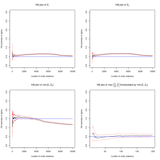
To check whether we can get identify the distributions of 𝒀𝒀\boldsymbol{Y} and 𝑽𝑽\boldsymbol{V} from a data sample of 𝒁=𝒀+𝑽𝒁𝒀𝑽\boldsymbol{Z}=\boldsymbol{Y}+\boldsymbol{V}, we simulate data following this model for three different choices of α𝛼\alpha while keeping α0subscript𝛼0\alpha_{0} fixed. We then check whether we can estimate back the values of α𝛼\alpha and α0subscript𝛼0\alpha_{0}. In all the three cases α0=2subscript𝛼02\alpha_{0}=2 with Θ1=dΘ2superscriptdsubscriptΘ1subscriptΘ2\Theta_{1}\stackrel{{\scriptstyle\lower 0.60275pt\hbox{$\scriptscriptstyle\mathrm{d}$}}}{{=}}\Theta_{2} with (Θ11)subscriptΘ11(\Theta_{1}-1) following an iid standard exponential distribution and p=0.5𝑝0.5p=0.5. In each case we simulate 10000 iid samples from 𝒁𝒁\boldsymbol{Z}. Then we create Hill plots for the marginals of Z1subscript𝑍1Z_{1} and Z2subscript𝑍2Z_{2} to identify the value of α𝛼\alpha. To detect the hidden part we create a Hill plot for min(Z1,Z2)subscript𝑍1subscript𝑍2\min(Z_{1},Z_{2}) to find the value of α0subscript𝛼0\alpha_{0}. Referencing (1.12), we also make a QQ plot of max(Z1/Z2,Z2/Z1)subscript𝑍1subscript𝑍2subscript𝑍2subscript𝑍1\max(Z_{1}/Z_{2},Z_{2}/Z_{1}) for the 100 highest values of min(Z1,Z2)subscript𝑍1subscript𝑍2\min(Z_{1},Z_{2}) against the quantiles of standard exponential which is the distribution of Θ1subscriptΘ1\Theta_{1} and Θ2subscriptΘ2\Theta_{2}. We discuss the cases below.

  1. Case 1:

    α=1𝛼1\alpha=1. The top panel of Figure 1 indicates that we can identify the tails of 𝒁𝒁\boldsymbol{Z} to be heavy tailed. The correct index α=1𝛼1\alpha=1 is slightly overestimated. The Hill plot of min(Z1,Z2)subscript𝑍1subscript𝑍2\min(Z_{1},Z_{2}) also indicates HRV on 𝔼0subscript𝔼0\mathbb{E}_{0} with index close to α0=2subscript𝛼02\alpha_{0}=2. The QQ plot of max(Z1/Z2,Z2/Z1)subscript𝑍1subscript𝑍2subscript𝑍2subscript𝑍1\max(Z_{1}/Z_{2},Z_{2}/Z_{1}) thresholded by the 100 largest values of min(Z1,Z2)subscript𝑍1subscript𝑍2\min(Z_{1},Z_{2}) against standard exponential shows a decent fit.

    Refer to caption
    Figure 1. Exploratory plots for Example 3.1, case 1, with α=1,α0=2formulae-sequence𝛼1subscript𝛼02\alpha=1,\alpha_{0}=2. Top panel: Hill plots for the marginals Z1subscript𝑍1Z_{1} and Z2subscript𝑍2Z_{2}. Bottom left: Hill plot for min{Z1,Z2}subscript𝑍1subscript𝑍2\min{\{Z_{1},Z_{2}\}}. Bottom right: exponential QQ plot of max{Z1/Z2,Z2/Z1}subscript𝑍1subscript𝑍2subscript𝑍2subscript𝑍1\max{\{Z_{1}/Z_{2},Z_{2}/Z_{1}\}} thresholded by the 100 largest values of min{Z1,Z2}subscript𝑍1subscript𝑍2\min\{Z_{1},Z_{2}\}.
  2. Case 2:

    α=1.5𝛼1.5\alpha=1.5. The top panel of Figure 2 again indicates that we can identify the tails of 𝒁𝒁\boldsymbol{Z} to be heavy tailed. The index α𝛼\alpha is again overestimated, this time more than in the previous case, perhaps because of the closeness of α𝛼\alpha to α0subscript𝛼0\alpha_{0}. The Hill plot of min{Z1,Z2}subscript𝑍1subscript𝑍2\min\{Z_{1},Z_{2}\} also indicates HRV on 𝔼0subscript𝔼0\mathbb{E}_{0} with index close to α0=2subscript𝛼02\alpha_{0}=2. The QQ plot of max{Z1/Z2,Z2/Z1}subscript𝑍1subscript𝑍2subscript𝑍2subscript𝑍1\max\{Z_{1}/Z_{2},Z_{2}/Z_{1}\} thresholded by the 100 largest values of min{Z1,Z2}subscript𝑍1subscript𝑍2\min\{Z_{1},Z_{2}\} against standard exponential shows a decent fit again.

    Refer to caption
    Figure 2. Exploratory plots for Example 3.1, case 2, with α=1.5,α0=2formulae-sequence𝛼1.5subscript𝛼02\alpha=1.5,\alpha_{0}=2. Top panel: Hill plots for the marginals Z1subscript𝑍1Z_{1} and Z2subscript𝑍2Z_{2}. Bottom left: Hill plot for min{Z1,Z2}subscript𝑍1subscript𝑍2\min\{Z_{1},Z_{2}\}. Bottom right: exponential QQ plot of max{Z1/Z2,Z2/Z1}subscript𝑍1subscript𝑍2subscript𝑍2subscript𝑍1\max\{Z_{1}/Z_{2},Z_{2}/Z_{1}\} thresholded by the 100 largest values of min{Z1,Z2}subscript𝑍1subscript𝑍2\min\{Z_{1},Z_{2}\}.
  3. Case 3:

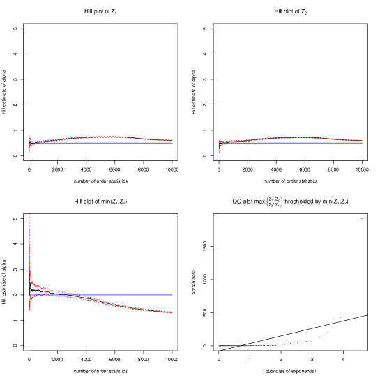
    α=0.5𝛼0.5\alpha=0.5. In this case too, the top panel of Figure 3 indicates heavy tailed behavior of 𝒁𝒁\boldsymbol{Z}. The Hill plot of min(Z1,Z2)subscript𝑍1subscript𝑍2\min(Z_{1},Z_{2}) also indicates hidden regular variation. The indices α=0.5𝛼0.5\alpha=0.5 and α0=2subscript𝛼02\alpha_{0}=2 are reasonably estimated here, presumably because the original values of α𝛼\alpha and α0subscript𝛼0\alpha_{0} are far apart. However, the exponential QQ plot of max{Z1/Z2,Z2/Z1}subscript𝑍1subscript𝑍2subscript𝑍2subscript𝑍1\max\{Z_{1}/Z_{2},Z_{2}/Z_{1}\} for the 100 largest values of min{Z1,Z2}subscript𝑍1subscript𝑍2\min\{Z_{1},Z_{2}\} struggles to indicate an exponential fit.
    Refer to caption
    Figure 3. Exploratory plots for Example 3.1, case 3, with α=0.5,α0=2formulae-sequence𝛼0.5subscript𝛼02\alpha=0.5,\alpha_{0}=2. Top panel: Hill plots for the marginals Z1subscript𝑍1Z_{1} and Z2subscript𝑍2Z_{2}. Bottom left: Hill plot for min{Z1,Z2}subscript𝑍1subscript𝑍2\min\{Z_{1},Z_{2}\}. Bottom right: exponential QQ plot of max{Z1/Z2,Z2/Z1}subscript𝑍1subscript𝑍2subscript𝑍2subscript𝑍1\max\{Z_{1}/Z_{2},Z_{2}/Z_{1}\} thresholded by the 100 maximum values of min(Z1,Z2)subscript𝑍1subscript𝑍2\min(Z_{1},Z_{2}).

3.2.2. What happens if 𝒀𝒀\boldsymbol{Y} has HRV but 𝑽𝑽\boldsymbol{V} has no HRV

In Proposition 3.1, we can remove the restriction that 𝒀=(Y1,Y2)𝒀subscript𝑌1subscript𝑌2\boldsymbol{Y}=(Y_{1},Y_{2}) concentrates on the axes at the expense of a tail condition on 𝒀𝒀\boldsymbol{Y} that guarantees the tails of 𝑽𝑽\boldsymbol{V} and 𝒀𝒀\boldsymbol{Y} do not interact in such as way as to obscure the fact that the hidden angular measure of 𝒁𝒁\boldsymbol{Z} is that of 𝑽𝑽\boldsymbol{V}. Continue to suppose 𝒁=𝒀+𝑽𝒁𝒀𝑽\boldsymbol{Z}=\boldsymbol{Y}+\boldsymbol{V} with 𝒀𝑽perpendicular-toabsentperpendicular-to𝒀𝑽\boldsymbol{Y}\mathchoice{\mathrel{\hbox to0.0pt{$\displaystyle\perp$\hss}\mkern 2.0mu{\displaystyle\perp}}}{\mathrel{\hbox to0.0pt{$\textstyle\perp$\hss}\mkern 2.0mu{\textstyle\perp}}}{\mathrel{\hbox to0.0pt{$\scriptstyle\perp$\hss}\mkern 2.0mu{\scriptstyle\perp}}}{\mathrel{\hbox to0.0pt{$\scriptscriptstyle\perp$\hss}\mkern 2.0mu{\scriptscriptstyle\perp}}}\boldsymbol{V}.

Proposition 3.2.

Suppose

  1. (1)

    𝒀MRV(α,b(t),ν,𝔼)𝒀MRV𝛼𝑏𝑡𝜈𝔼\boldsymbol{Y}\in\text{MRV}(\alpha,b(t),\nu,\mathbb{E}) and exhibits asymptotic independence.

  2. (2)

    𝑽𝑽\boldsymbol{V} has MRVon 𝔼𝔼\mathbb{E} (not 𝔼0subscript𝔼0\mathbb{E}_{0}) with index α0αsubscript𝛼0𝛼\alpha_{0}\geqslant\alpha, scaling function b0(t)=o(b(t))subscript𝑏0𝑡𝑜𝑏𝑡b_{0}(t)=o(b(t)), limit measure ν0M(𝔼)subscript𝜈0𝑀𝔼\nu_{0}\in M(\mathbb{E}) with no asymptotic independence so that

    t𝐏[𝑽/b0(t)]ν0 in 𝕄(𝔼).𝑡𝐏delimited-[]𝑽subscript𝑏0𝑡subscript𝜈0 in 𝕄𝔼t\mathbf{P}[\boldsymbol{V}/b_{0}(t)\in\cdot\,]\to\nu_{0}\quad\text{ in }\mathbb{M}(\mathbb{E}).
  3. (3)

    The interaction of the tails of 𝒀𝒀\boldsymbol{Y} and 𝑽𝑽\boldsymbol{V} is controlled by the condition

    (3.6) t𝐏[Y1Y2>b0(t)x]0,t,x>0.formulae-sequence𝑡𝐏delimited-[]subscript𝑌1subscript𝑌2subscript𝑏0𝑡𝑥0formulae-sequence𝑡𝑥0t\mathbf{P}[Y_{1}\wedge Y_{2}>b_{0}(t)x]\to 0,\quad t\to\infty,\,x>0.

Then 𝐙=𝐘+𝐕𝐙𝐘𝐕\boldsymbol{Z}=\boldsymbol{Y}+\boldsymbol{V} has

  1. (1)

    MRV(α,b(t),ν,𝔼)MRV𝛼𝑏𝑡𝜈𝔼\text{MRV}(\alpha,b(t),\nu,\mathbb{E}) and asymptotic independence.

  2. (2)

    HRV on 𝔼0subscript𝔼0\mathbb{E}_{0} with index α0subscript𝛼0\alpha_{0}, scaling function b0(t)subscript𝑏0𝑡b_{0}(t), limit measure ν0subscript𝜈0\nu_{0} restricted to 𝔼0subscript𝔼0\mathbb{E}_{0}.

Remarks: For the 𝒀𝒀\boldsymbol{Y} defined in Proposition 3.1, Y1Y2=0subscript𝑌1subscript𝑌20Y_{1}\wedge Y_{2}=0 so (3.6) is automatic. If Y1,Y2subscript𝑌1subscript𝑌2Y_{1},Y_{2} are iid with 𝐏[Yi>x]RVα𝐏delimited-[]subscript𝑌𝑖𝑥𝑅subscript𝑉𝛼\mathbf{P}[Y_{i}>x]\in RV_{-\alpha}, 𝒀𝒀\boldsymbol{Y} itself has HRV [22, 23] with index α0=2αsubscript𝛼02𝛼\alpha_{0}=2\alpha and condition (3.6) is needed to guarantee the HRV of 𝒁𝒁\boldsymbol{Z} comes from 𝑽𝑽\boldsymbol{V} and not 𝒀𝒀\boldsymbol{Y}. Condition (3.6) is equivalent in this case to

(3.7) (𝐏[Y1>x])2𝐏[V1V2>x]0,(x).superscript𝐏delimited-[]subscript𝑌1𝑥2𝐏delimited-[]subscript𝑉1subscript𝑉2𝑥0𝑥\frac{(\mathbf{P}[Y_{1}>x])^{2}}{\mathbf{P}[V_{1}\wedge V_{2}>x]}\to 0,\quad(x\to\infty).

and it is sufficient that

α02<α<α0.subscript𝛼02𝛼subscript𝛼0\frac{\alpha_{0}}{2}<\alpha<\alpha_{0}.

This is seen by noting that for Y1,Y2subscript𝑌1subscript𝑌2Y_{1},Y_{2} iid index α𝛼\alpha, (3.6) is

t(𝐏[Y1>b0(t)x])2=𝑡superscript𝐏delimited-[]subscript𝑌1subscript𝑏0𝑡𝑥2absent\displaystyle t\Bigl{(}\mathbf{P}[Y_{1}>b_{0}(t)x]\Bigr{)}^{2}= t(𝐏[Y1>b(b(b0(t)))x])2𝑡superscript𝐏delimited-[]subscript𝑌1𝑏superscript𝑏subscript𝑏0𝑡𝑥2\displaystyle t\Bigl{(}\mathbf{P}[Y_{1}>b\bigl{(}b^{\leftarrow}(b_{0}(t))\bigr{)}x]\Bigr{)}^{2}
=\displaystyle= tb(b0(t))(b(b0(t))𝐏[Y1>b(b(b0(t)))x])2𝑡superscript𝑏subscript𝑏0𝑡superscriptsuperscript𝑏subscript𝑏0𝑡𝐏delimited-[]subscript𝑌1𝑏superscript𝑏subscript𝑏0𝑡𝑥2\displaystyle\frac{t}{b^{\leftarrow}(b_{0}(t))}\Bigl{(}b^{\leftarrow}(b_{0}(t))\mathbf{P}[Y_{1}>b\bigl{(}b^{\leftarrow}(b_{0}(t))\bigr{)}x]\Bigr{)}^{2}
and since b(b0(t))superscript𝑏subscript𝑏0𝑡b^{\leftarrow}(b_{0}(t))\to\infty and b()𝑏b(\cdot) is the scaling function of Y1subscript𝑌1Y_{1}, this is asymptotic to
similar-to\displaystyle\sim tb(b0(t))x2α.𝑡superscript𝑏subscript𝑏0𝑡superscript𝑥2𝛼\displaystyle\frac{t}{b^{\leftarrow}(b_{0}(t))}x^{-2\alpha}.

We need limtt/b(b0(t))=0subscript𝑡𝑡superscript𝑏subscript𝑏0𝑡0\lim_{t\to\infty}{t}/{b^{\leftarrow}(b_{0}(t))}=0 and unwinding this condition yields (3.7).

Proof.

As in Proposition 3.1, we focus on the HRV claim. Again assume f𝒞((0,)2)𝑓𝒞superscript02f\in\mathcal{C}((0,\infty)^{2}) and f𝑓f is bounded by fnorm𝑓\|f\|, uniformly continuous with

f(𝒙)=0, if x1x2<η,formulae-sequence𝑓𝒙0 if subscript𝑥1subscript𝑥2𝜂f(\boldsymbol{x})=0,\quad\text{ if }x_{1}\wedge x_{2}<\eta,

for some η>0𝜂0\eta>0. We need to show (3.5). For any small δ>0𝛿0\delta>0 with δ<η𝛿𝜂\delta<\eta, the absolute value of the difference in (3.5) is

tE||1[Y1Y2>b0(t)δ]+tE||1[Y1Y2<b0(t)δ,V1V2>b0(t)(ηδ)]=I+II,tE|\cdot|1_{[Y_{1}\vee Y_{2}>b_{0}(t)\delta]}+tE|\cdot|1_{[Y_{1}\vee Y_{2}<b_{0}(t)\delta,V_{1}\wedge V_{2}>b_{0}(t)(\eta-\delta)]}=I+II,

since for the second term, the only way the difference can be non-zero is if 𝑽𝑽\boldsymbol{V} is sufficiently large. Term II is dominated by

II𝐼𝐼absent\displaystyle{II}\leqslant ωf(δ)t𝐏[V1V2>b0(t)(ηδ)]subscript𝜔𝑓𝛿𝑡𝐏delimited-[]subscript𝑉1subscript𝑉2subscript𝑏0𝑡𝜂𝛿\displaystyle\omega_{f}(\delta)t\mathbf{P}[V_{1}\wedge V_{2}>b_{0}(t)(\eta-\delta)]
similar-to\displaystyle\sim ωf(δ)(const)(ηδ)α0,(t)subscript𝜔𝑓𝛿𝑐𝑜𝑛𝑠𝑡superscript𝜂𝛿subscript𝛼0𝑡\displaystyle\omega_{f}(\delta)(const)(\eta-\delta)^{-\alpha_{0}},\quad(t\to\infty)
\displaystyle\to 0, as δ0.0 as 𝛿0\displaystyle 0,\qquad\text{ as }\delta\to 0.

For I𝐼I we have

I𝐼absent\displaystyle I\leqslant tE||(1[Y1Y2>b0(t)δ]]+1[Y1>b0(t)δ,Y2b0(t)δ]]+1[Y2>b0(t)δ,Y1<b0(t)δ]])\displaystyle tE|\cdot|\Bigl{(}1_{[Y_{1}\wedge Y_{2}>b_{0}(t)\delta]]}+1_{[Y_{1}>b_{0}(t)\delta,Y_{2}\leqslant b_{0}(t)\delta]]}+1_{[Y_{2}>b_{0}(t)\delta,Y_{1}<b_{0}(t)\delta]]}\Bigr{)}
=\displaystyle= Ia+Ib+Ic.𝐼𝑎𝐼𝑏𝐼𝑐\displaystyle Ia+Ib+Ic.

The term Ia𝐼𝑎Ia can be quickly killed,

Ia2ft𝐏[Y1Y2>b0(t)δ]0,(t)formulae-sequence𝐼𝑎2norm𝑓𝑡𝐏delimited-[]subscript𝑌1subscript𝑌2subscript𝑏0𝑡𝛿0𝑡Ia\leqslant 2\|f\|t\mathbf{P}[Y_{1}\wedge Y_{2}>b_{0}(t)\delta]\to 0,\quad(t\to\infty)

from (3.6). The term Ib𝐼𝑏Ib is dominated by

Ib𝐼𝑏absent\displaystyle Ib\leqslant 2ft𝐏[Y1>b0(t)δ,V2>b0(t)(ηδ)]2norm𝑓𝑡𝐏delimited-[]formulae-sequencesubscript𝑌1subscript𝑏0𝑡𝛿subscript𝑉2subscript𝑏0𝑡𝜂𝛿\displaystyle 2\|f\|t\mathbf{P}[Y_{1}>b_{0}(t)\delta,V_{2}>b_{0}(t)(\eta-\delta)]
=\displaystyle= 2ft𝐏[V2>b0(t)(ηδ)]𝐏[Y1>b0(t)δ]2norm𝑓𝑡𝐏delimited-[]subscript𝑉2subscript𝑏0𝑡𝜂𝛿𝐏delimited-[]subscript𝑌1subscript𝑏0𝑡𝛿\displaystyle 2\|f\|t\mathbf{P}[V_{2}>b_{0}(t)(\eta-\delta)]\mathbf{P}[Y_{1}>b_{0}(t)\delta]
similar-to\displaystyle\sim f(ηδ)α0𝐏[Y1>b0(t)δ](t),norm𝑓superscript𝜂𝛿subscript𝛼0𝐏delimited-[]subscript𝑌1subscript𝑏0𝑡𝛿𝑡\displaystyle\|f\|(\eta-\delta)^{-\alpha_{0}}\mathbf{P}[Y_{1}>b_{0}(t)\delta]\quad(t\to\infty),
\displaystyle\to 0(t).0𝑡\displaystyle 0\qquad(t\to\infty).

Term Ic𝐼𝑐Ic is handled similarly. ∎

3.2.3. What happens if 𝒀𝒀\boldsymbol{Y} has no HRV but 𝑽𝑽\boldsymbol{V} has HRV

A problem with the additive model is the tail weights contributing to MRV on 𝔼𝔼\mathbb{E} and HRV on 𝔼0subscript𝔼0\mathbb{E}_{0} can be confounded between 𝒀𝒀\boldsymbol{Y} and 𝑽𝑽\boldsymbol{V} and it is possible for 𝑽𝑽\boldsymbol{V} to have MRV on 𝔼𝔼\mathbb{E}, HRV on 𝔼0subscript𝔼0\mathbb{E}_{0} but the hidden measure of 𝒁=𝒀+𝑽𝒁𝒀𝑽\boldsymbol{Z}=\boldsymbol{Y}+\boldsymbol{V} is not the hidden measure of 𝑽𝑽\boldsymbol{V}.

To focus on the influence of 𝑽𝑽\boldsymbol{V}, we again assume 𝒀𝒀\boldsymbol{Y} has the structure (3.1) used in Proposition 3.1.

Proposition 3.3.

Suppose

  1. (1)

    𝒀𝒀\boldsymbol{Y} has form (3.1) where ξ1,ξ2subscript𝜉1subscript𝜉2\xi_{1},\xi_{2} are iid, each with distributions having regularly varying tails with index α𝛼\alpha and scaling function b(t)𝑏𝑡b(t).

  2. (2)

    𝑽𝑽\boldsymbol{V} has both MRV on 𝔼𝔼\mathbb{E} and HRV on 𝔼0subscript𝔼0\mathbb{E}_{0}:

    1. (a)

      𝑽MRV(α,b(t),ν,𝔼)𝑽MRVsubscript𝛼subscript𝑏𝑡𝜈𝔼\boldsymbol{V}\in\text{MRV}(\alpha_{*},b_{*}(t),\nu,\mathbb{E}) and has asymptotic independence.

    2. (b)

      𝑽MRV(α0,b0(t),ν0,𝔼0)𝑽MRVsubscript𝛼0subscript𝑏0𝑡subscript𝜈0subscript𝔼0\boldsymbol{V}\in\text{MRV}(\alpha_{0},b_{0}(t),\nu_{0},\mathbb{E}_{0}).

  3. (3)

    The parameters α,α,α0𝛼subscript𝛼subscript𝛼0\alpha,\,\alpha_{*},\,\alpha_{0} are related by ααα0𝛼subscript𝛼subscript𝛼0\alpha\leqslant\alpha_{*}\leqslant\alpha_{0} and the scaling functions b(t),b(t),b0(t)𝑏𝑡subscript𝑏𝑡subscript𝑏0𝑡b(t),b_{*}(t),b_{0}(t) satisfy b(t)=o(b(t)),b0(t)=o(b(t))formulae-sequencesubscript𝑏𝑡𝑜𝑏𝑡subscript𝑏0𝑡𝑜subscript𝑏𝑡b_{*}(t)=o(b(t)),\,b_{0}(t)=o(b_{*}(t)).

  4. (4)

    Define a scaling function h(t)𝑡h(t) through its inverse h(t)superscript𝑡h^{\leftarrow}(t) by

    (3.8) h(t)=:b(t)b(t)(const)1𝐏[ξ1>t]𝐏[V1>t].h^{\leftarrow}(t)=:b^{\leftarrow}(t)b_{*}^{\leftarrow}(t)\sim(const)\frac{1}{\mathbf{P}[\xi_{1}>t]\mathbf{P}[V_{1}>t]}.

Then

  1. (1)

    If

    (3.9) h(t)/b0(t),𝑡subscript𝑏0𝑡h(t)/b_{0}(t)\to\infty,

    𝒁MRV(α,b(t),ν,𝔼)𝒁MRV𝛼𝑏𝑡𝜈𝔼\boldsymbol{Z}\in\text{MRV}(\alpha,b(t),\nu,\mathbb{E}) with asymptotic independence and has HRV on 𝔼0subscript𝔼0\mathbb{E}_{0} with index α+α𝛼subscript𝛼\alpha+\alpha_{*} and limit measure (different than the hidden measure of 𝑽𝑽\boldsymbol{V}):

    (3.10) ν𝒁,hidden:=12(να×να+να×να).assignsubscript𝜈𝒁hidden12subscript𝜈𝛼subscript𝜈subscript𝛼subscript𝜈subscript𝛼subscript𝜈𝛼\nu_{\boldsymbol{Z},\text{hidden}}:=\frac{1}{2}\bigl{(}\nu_{\alpha}\times\nu_{\alpha_{*}}+\nu_{\alpha_{*}}\times\nu_{\alpha}\bigr{)}.

    A sufficient condition for (3.9) is α<α0α.subscript𝛼subscript𝛼0𝛼\alpha_{*}<\alpha_{0}-\alpha.

  2. (2)

    If

    (3.11) h(t)/b0(t)0,𝑡subscript𝑏0𝑡0h(t)/b_{0}(t)\to 0,

    then 𝒁MRV(α,b(t),ν,𝔼)MRV(α0,b0(t),ν0,𝔼0)𝒁MRV𝛼𝑏𝑡𝜈𝔼MRVsubscript𝛼0subscript𝑏0𝑡subscript𝜈0subscript𝔼0\boldsymbol{Z}\in\text{MRV}(\alpha,b(t),\nu,\mathbb{E})\cap\text{MRV}(\alpha_{0},b_{0}(t),\nu_{0},\mathbb{E}_{0}) and 𝒁𝒁\boldsymbol{Z} has asymptotic independence and has HRV and the hidden limit measure ν0subscript𝜈0\nu_{0} of 𝒁𝒁\boldsymbol{Z} is the hidden measure of 𝑽𝑽\boldsymbol{V}. A sufficient condition for (3.11) is α>α0αsubscript𝛼subscript𝛼0𝛼\alpha_{*}>\alpha_{0}-\alpha

  3. (3)

    If

    (3.12) h(t)/b0(t)c(0,),𝑡subscript𝑏0𝑡𝑐0h(t)/b_{0}(t)\to c\in(0,\infty),

    then 𝒁MRV(α,b(t),ν,𝔼\boldsymbol{Z}\in\text{MRV}(\alpha,b(t),\nu,\mathbb{E}) with asymptotic independence and 𝒁𝒁\boldsymbol{Z} has HRV with index α+α𝛼subscript𝛼\alpha+\alpha_{*} and hidden measure which is a sum of the measure given in (3.10) and ν0subscript𝜈0\nu_{0}, the hidden measure of 𝑽𝑽\boldsymbol{V},

    (3.13) ν𝒁subscript𝜈𝒁\displaystyle\nu_{\boldsymbol{Z}} =12(να×να+να×να)+ν0.absent12subscript𝜈𝛼subscript𝜈subscript𝛼subscript𝜈subscript𝛼subscript𝜈𝛼subscript𝜈0\displaystyle=\frac{1}{2}\bigl{(}\nu_{\alpha}\times\nu_{\alpha_{*}}+\nu_{\alpha_{*}}\times\nu_{\alpha}\bigr{)}+\nu_{0}.

    A sufficient condition for (3.11) is α=α0α.subscript𝛼subscript𝛼0𝛼\alpha_{*}=\alpha_{0}-\alpha.

Proof.

Begin with the following observations for all cases: As t𝑡t\to\infty,

(3.14) t𝐏[(ξ1h(t),V2h(t))]να×να𝑡𝐏delimited-[]subscript𝜉1𝑡subscript𝑉2𝑡subscript𝜈𝛼subscript𝜈subscript𝛼\displaystyle t\mathbf{P}[\Bigl{(}\frac{\xi_{1}}{h(t)},\frac{V_{2}}{h(t)}\Bigr{)}\in\cdot\,]\to\nu_{\alpha}\times\nu_{\alpha_{*}}
(3.15) t𝐏[(V1h(t),ξ2h(t))]να×να𝑡𝐏delimited-[]subscript𝑉1𝑡subscript𝜉2𝑡subscript𝜈subscript𝛼subscript𝜈𝛼\displaystyle t\mathbf{P}[\Bigl{(}\frac{V_{1}}{h(t)},\frac{\xi_{2}}{h(t)}\Bigr{)}\in\cdot\,]\to\nu_{\alpha_{*}}\times\nu_{\alpha}

in 𝕄((0,)2)𝕄superscript02\mathbb{M}((0,\infty)^{2}). To see this, write for x>0,y>0formulae-sequence𝑥0𝑦0x>0,\,y>0,

t𝐏[ξ1>h(t)x,\displaystyle t\mathbf{P}[\xi_{1}>h(t)x, V2>h(t)y]=t𝐏[ξ1>bb(h)x]𝐏[V2>bb(h)y]\displaystyle V_{2}>h(t)y]=t\mathbf{P}[\xi_{1}>b\circ b^{\leftarrow}(h)x]\mathbf{P}[V_{2}>b_{*}\circ b_{*}^{\leftarrow}(h)y]
=\displaystyle= tb(h)b(h)b(h)𝐏[ξ1>bb(h)x]𝑡superscript𝑏superscriptsubscript𝑏superscript𝑏𝐏delimited-[]subscript𝜉1𝑏superscript𝑏𝑥\displaystyle\frac{t}{b^{\leftarrow}(h)b_{*}^{\leftarrow}(h)}b^{\leftarrow}(h)\mathbf{P}[\xi_{1}>b\circ b^{\leftarrow}(h)x]
b(h)𝐏[V2>bb(h)y]superscriptsubscript𝑏𝐏delimited-[]subscript𝑉2subscript𝑏superscriptsubscript𝑏𝑦\displaystyle\qquad\qquad b_{*}^{\leftarrow}(h)\mathbf{P}[V_{2}>b_{*}\circ b_{*}^{\leftarrow}(h)y]
similar-to\displaystyle\sim tb(h)b(h)xαyα𝑡superscript𝑏superscriptsubscript𝑏superscript𝑥𝛼superscript𝑦subscript𝛼\displaystyle\frac{t}{b^{\leftarrow}(h)b_{*}^{\leftarrow}(h)}x^{-\alpha}y^{-\alpha_{*}}
similar-to\displaystyle\sim να(x,)να(y,).subscript𝜈𝛼𝑥subscript𝜈subscript𝛼𝑦\displaystyle\nu_{\alpha}(x,\infty)\nu_{\alpha_{*}}(y,\infty).

The proof of (3.15) is the same.

Now assume f𝒞((0,)2)𝑓𝒞superscript02f\in\mathcal{C}((0,\infty)^{2}) and f𝑓f is bounded by fnorm𝑓\|f\|, uniformly continuous with

f(𝒙)=0, if x1x2<η,formulae-sequence𝑓𝒙0 if subscript𝑥1subscript𝑥2𝜂f(\boldsymbol{x})=0,\quad\text{ if }x_{1}\wedge x_{2}<\eta,

for some η>0𝜂0\eta>0. Write

(3.16) tEf(𝒀+𝑽h(t))=t2Ef(ξ1+V1h(t),V2h(t))+t2Ef(V1h(t),ξ2+V2h(t))=A+B𝑡𝐸𝑓𝒀𝑽𝑡𝑡2𝐸𝑓subscript𝜉1subscript𝑉1𝑡subscript𝑉2𝑡𝑡2𝐸𝑓subscript𝑉1𝑡subscript𝜉2subscript𝑉2𝑡𝐴𝐵tEf\Bigl{(}\frac{\boldsymbol{Y}+\boldsymbol{V}}{h(t)}\Bigr{)}=\frac{t}{2}Ef\Bigl{(}\frac{\xi_{1}+V_{1}}{h(t)},\frac{V_{2}}{h(t)}\Bigr{)}+\frac{t}{2}Ef\Bigl{(}\frac{V_{1}}{h(t)},\frac{\xi_{2}+V_{2}}{h(t)}\Bigr{)}=A+B

For case (1) where (3.9) holds, we get a limit for A𝐴A by writing

tE|f(ξ1+V1h(t),V2h(t))\displaystyle tE\Bigl{|}f\Bigl{(}\frac{\xi_{1}+V_{1}}{h(t)},\frac{V_{2}}{h(t)}\Bigr{)}- f(ξ1h(t),V2h(t))|=tE||1[V1<h(t)δ,ξ1>h(t)(ηδ),V2>h(t)η]\displaystyle f\Bigl{(}\frac{\xi_{1}}{h(t)},\frac{V_{2}}{h(t)}\Bigr{)}\Bigr{|}=tE\Bigl{|}\cdot\Bigr{|}1_{[V_{1}<h(t)\delta,\xi_{1}>h(t)(\eta-\delta),V_{2}>h(t)\eta]}
+tE||1V1>h(t)δ,V2>h(t)η]=I+II.\displaystyle+tE\Bigl{|}\cdot\Bigr{|}1_{V_{1}>h(t)\delta,V_{2}>h(t)\eta]}=I+II.

Now

I𝐼absent\displaystyle I\leqslant ωf(δ)t𝐏[ξ1>h(t)(ηδ),V2>h(t)η]subscript𝜔𝑓𝛿𝑡𝐏delimited-[]formulae-sequencesubscript𝜉1𝑡𝜂𝛿subscript𝑉2𝑡𝜂\displaystyle\omega_{f}(\delta)t\mathbf{P}[\xi_{1}>h(t)(\eta-\delta),V_{2}>h(t)\eta]
\displaystyle\to ωf(δ)να((ηδ),)να(η,)subscript𝜔𝑓𝛿subscript𝜈𝛼𝜂𝛿subscript𝜈subscript𝛼𝜂\displaystyle\omega_{f}(\delta)\nu_{\alpha}((\eta-\delta),\infty)\nu_{\alpha_{*}}(\eta,\infty)
from (3.14)
\displaystyle\to 0(δ0).0𝛿0\displaystyle 0\qquad(\delta\to 0).

We can control II𝐼𝐼II by observing

II𝐼𝐼absent\displaystyle II\leqslant 2ft𝐏[V1>h(t)δ,V2>h(t)η]2norm𝑓𝑡𝐏delimited-[]formulae-sequencesubscript𝑉1𝑡𝛿subscript𝑉2𝑡𝜂\displaystyle 2\|f\|t\mathbf{P}[V_{1}>h(t)\delta,V_{2}>h(t)\eta]
\displaystyle\leqslant 2ftb0(h(t))b0(h(t))𝐏[V1V2>b0b0(h(t))δη]2norm𝑓𝑡superscriptsubscript𝑏0𝑡superscriptsubscript𝑏0𝑡𝐏delimited-[]subscript𝑉1subscript𝑉2subscript𝑏0superscriptsubscript𝑏0𝑡𝛿𝜂\displaystyle 2\|f\|\frac{t}{b_{0}^{\leftarrow}(h(t))}b_{0}^{\leftarrow}(h(t))\mathbf{P}[V_{1}\wedge V_{2}>b_{0}\circ b_{0}^{\leftarrow}(h(t))\delta\wedge\eta]
\displaystyle\to 0(t),0𝑡\displaystyle 0\qquad(t\to\infty),

from (3.9). The second term of (3.10) comes from B𝐵B in a similar way to the derivation of A𝐴A, relying on (3.15). This completes case (1) where (3.9) holds.

For Case (2) when (3.11) holds, replace h(t)𝑡h(t) with b0(t)subscript𝑏0𝑡b_{0}(t) in (3.16) and focus on A𝐴A. We compare with f(𝑽/b0(t))𝑓𝑽subscript𝑏0𝑡f(\boldsymbol{V}/b_{0}(t)):

t𝐄|f(\displaystyle t\mathbf{E}\Bigl{|}f\Bigl{(} ξ1+V1b0(t),V2b0(t))f(𝑽b0(t))|\displaystyle\frac{\xi_{1}+V_{1}}{b_{0}(t)},\frac{V_{2}}{b_{0}(t)}\Bigr{)}-f\Bigl{(}\frac{\boldsymbol{V}}{b_{0}(t)}\Bigr{)}\Bigr{|}
=\displaystyle= t𝐄||1[ξ1<b0(t)δ,V1>b0(ηδ),V2>b0η]+t𝐄||1[ξ1>b0(t)δ,V2>b0η]=I+II.\displaystyle t\mathbf{E}|\cdot|1_{[\xi_{1}<b_{0}(t)\delta,V_{1}>b_{0}(\eta-\delta),V_{2}>b_{0}\eta]}+t\mathbf{E}|\cdot|1_{[\xi_{1}>b_{0}(t)\delta,V_{2}>b_{0}\eta]}=I+II.

Since t𝐄f(𝑽/b0(t))f𝑑ν0,𝑡𝐄𝑓𝑽subscript𝑏0𝑡𝑓differential-dsubscript𝜈0t\mathbf{E}f(\boldsymbol{V}/b_{0}(t))\to\int fd\nu_{0}, we only have to show that both I𝐼I and II𝐼𝐼II go to zero. For I𝐼I we have

I𝐼absent\displaystyle I\leqslant ωf(δ)t𝐏[V1V2>bo(t)(ηδ)η]ωf(δ)((ηδ)η)α0subscript𝜔𝑓𝛿𝑡𝐏delimited-[]subscript𝑉1subscript𝑉2subscript𝑏𝑜𝑡𝜂𝛿𝜂subscript𝜔𝑓𝛿superscript𝜂𝛿𝜂subscript𝛼0\displaystyle\omega_{f}(\delta)t\mathbf{P}[V_{1}\wedge V_{2}>b_{o}(t)(\eta-\delta)\wedge\eta]\to\omega_{f}(\delta)((\eta-\delta)\wedge\eta)^{-\alpha_{0}}
\displaystyle\to 0(δ0).0𝛿0\displaystyle 0\qquad(\delta\to 0).

Also using (3.11),

II2ftb(b0)b(b0)(b(b0)𝐏[ξ1>bb(b0)δ]b(b0)𝐏[V2>bb(b0)η])𝐼𝐼2norm𝑓𝑡superscript𝑏subscript𝑏0superscriptsubscript𝑏subscript𝑏0superscript𝑏subscript𝑏0𝐏delimited-[]subscript𝜉1𝑏superscript𝑏subscript𝑏0𝛿superscriptsubscript𝑏subscript𝑏0𝐏delimited-[]subscript𝑉2subscript𝑏superscriptsubscript𝑏subscript𝑏0𝜂\displaystyle II\leqslant 2\|f\|\frac{t}{b^{\leftarrow}(b_{0})b_{*}^{\leftarrow}(b_{0})}\Bigl{(}b^{\leftarrow}(b_{0})\mathbf{P}[\xi_{1}>b\circ b^{\leftarrow}(b_{0})\delta]b_{*}^{\leftarrow}(b_{0})\mathbf{P}[V_{2}>b_{*}\circ b_{*}^{\leftarrow}(b_{0})\eta]\Bigr{)}
(const)tb(b0)b(b0)=(const)th(b0)0.similar-toabsent𝑐𝑜𝑛𝑠𝑡𝑡superscript𝑏subscript𝑏0superscriptsubscript𝑏subscript𝑏0𝑐𝑜𝑛𝑠𝑡𝑡superscriptsubscript𝑏00\displaystyle\sim(const)\frac{t}{b^{\leftarrow}(b_{0})b_{*}^{\leftarrow}(b_{0})}=(const)\frac{t}{h^{\leftarrow}(b_{0})}\to 0.

We can deal with the term B𝐵B similarly so this completes treatment of Case (2).

Now consider Case (3) where (3.12) holds. Again replace h(t)𝑡h(t) by b0(t)subscript𝑏0𝑡b_{0}(t) in (3.16) and consider A𝐴A. Write

2A=2𝐴absent\displaystyle 2A= t𝐄f(ξ1+V1h(t),V2h(t))(1[ξ1b0(t)δ]+1[ξ1>b0(t)δ])𝑡𝐄𝑓subscript𝜉1subscript𝑉1𝑡subscript𝑉2𝑡subscript1delimited-[]subscript𝜉1subscript𝑏0𝑡𝛿subscript1delimited-[]subscript𝜉1subscript𝑏0𝑡𝛿\displaystyle t\mathbf{E}f\Bigl{(}\frac{\xi_{1}+V_{1}}{h(t)},\frac{V_{2}}{h(t)}\Bigr{)}\Bigl{(}1_{[\xi_{1}\leqslant b_{0}(t)\delta]}+1_{[\xi_{1}>b_{0}(t)\delta]}\Bigr{)}
=\displaystyle= t𝐄f(ξ1+V1h(t),V2h(t))f(𝑽h(t))1[ξ1b0(t)δ]𝑡𝐄𝑓subscript𝜉1subscript𝑉1𝑡subscript𝑉2𝑡𝑓𝑽𝑡subscript1delimited-[]subscript𝜉1subscript𝑏0𝑡𝛿\displaystyle t\mathbf{E}f\Bigl{(}\frac{\xi_{1}+V_{1}}{h(t)},\frac{V_{2}}{h(t)}\Bigr{)}-f\Bigl{(}\frac{\boldsymbol{V}}{h(t)}\Bigr{)}1_{[\xi_{1}\leqslant b_{0}(t)\delta]}
+t𝐄f(ξ1+V1h(t),V2h(t))f(ξ1h(t),V2h(t))1[ξ1>b0(t)δ]𝑡𝐄𝑓subscript𝜉1subscript𝑉1𝑡subscript𝑉2𝑡𝑓subscript𝜉1𝑡subscript𝑉2𝑡subscript1delimited-[]subscript𝜉1subscript𝑏0𝑡𝛿\displaystyle\qquad+t\mathbf{E}f\Bigl{(}\frac{\xi_{1}+V_{1}}{h(t)},\frac{V_{2}}{h(t)}\Bigr{)}-f\Bigl{(}\frac{\xi_{1}}{h(t)},\frac{V_{2}}{h(t)}\Bigr{)}1_{[\xi_{1}>b_{0}(t)\delta]}
+tEf(𝑽/b0(t))1[ξ1b0(t)δ]+t𝐄f(ξ1h(t),V2h(t))1[ξ1>b0(t)δ]𝑡𝐸𝑓𝑽subscript𝑏0𝑡subscript1delimited-[]subscript𝜉1subscript𝑏0𝑡𝛿𝑡𝐄𝑓subscript𝜉1𝑡subscript𝑉2𝑡subscript1delimited-[]subscript𝜉1subscript𝑏0𝑡𝛿\displaystyle\qquad+tEf(\boldsymbol{V}/b_{0}(t))1_{[\xi_{1}\leqslant b_{0}(t)\delta]}+t\mathbf{E}f\Bigl{(}\frac{\xi_{1}}{h(t)},\frac{V_{2}}{h(t)}\Bigr{)}1_{[\xi_{1}>b_{0}(t)\delta]}
=\displaystyle= a+b+c+d.𝑎𝑏𝑐𝑑\displaystyle a+b+c+d.

We have cf(𝒙)ν0(d𝒙)𝑐𝑓𝒙subscript𝜈0𝑑𝒙c\to\int f(\boldsymbol{x})\nu_{0}(d\boldsymbol{x}) since 𝐏[ξ1b0(t)δ]1.𝐏delimited-[]subscript𝜉1subscript𝑏0𝑡𝛿1\mathbf{P}[\xi_{1}\leqslant b_{0}(t)\delta]\to 1. For d𝑑d note

d=t𝐄f(ξ1h(t),V2h(t))f𝑑να×να𝑑𝑡𝐄𝑓subscript𝜉1𝑡subscript𝑉2𝑡𝑓differential-dsubscript𝜈𝛼subscript𝜈𝛼d=t\mathbf{E}f\Bigl{(}\frac{\xi_{1}}{h(t)},\frac{V_{2}}{h(t)}\Bigr{)}\to\int fd\nu_{\alpha}\times\nu_{\alpha*}

using (3.14) and the fact that (3.12) is equivalent to h(t)/b0(t)c1.superscript𝑡superscriptsubscript𝑏0𝑡superscript𝑐1h^{\leftarrow}(t)/b_{0}^{\leftarrow}(t)\to c^{-1}. Take the absolute value of a𝑎a and add to the indicator the event [V1>b0(t)(ηδ)]delimited-[]subscript𝑉1subscript𝑏0𝑡𝜂𝛿[V_{1}>b_{0}(t)(\eta-\delta)] (otherwise both terms in the difference are zero) and

|a|𝑎absent\displaystyle|a|\leqslant ωf(δ)t𝐏[V1V2>b0(t)(ηδ)]subscript𝜔𝑓𝛿𝑡𝐏delimited-[]subscript𝑉1subscript𝑉2subscript𝑏0𝑡𝜂𝛿\displaystyle\omega_{f}(\delta)t\mathbf{P}[V_{1}\wedge V_{2}>b_{0}(t)(\eta-\delta)]
\displaystyle\to ωf(δ)(ηδ)α0(t)subscript𝜔𝑓𝛿superscript𝜂𝛿subscript𝛼0𝑡\displaystyle\omega_{f}(\delta)(\eta-\delta)^{-\alpha_{0}}\quad(t\to\infty)
\displaystyle\to 0(δ0).0𝛿0\displaystyle 0\qquad(\delta\to 0).

For b𝑏b write

|b|𝑏absent\displaystyle|b|\leqslant t𝐄|f(ξ1+V1h(t),V2h(t))f(ξ1h(t),V2h(t))|1[ξ1>b0(t)δ,V1b0(t)δ]\displaystyle t\mathbf{E}\Bigl{|}f\Bigl{(}\frac{\xi_{1}+V_{1}}{h(t)},\frac{V_{2}}{h(t)}\Bigr{)}-f\Bigl{(}\frac{\xi_{1}}{h(t)},\frac{V_{2}}{h(t)}\Bigr{)}\Bigr{|}1_{[\xi_{1}>b_{0}(t)\delta,V_{1}\leqslant b_{0}(t)\delta]}
+t𝐄||1[ξ1>b0(t)δ,V1>b0(t)δ]=|b1|+|b2|.\displaystyle\qquad+t\mathbf{E}|\cdot|1_{[\xi_{1}>b_{0}(t)\delta,V_{1}>b_{0}(t)\delta]}=|b1|+|b2|.

We dominate |b1|𝑏1|b1| by using the modulus of continuity

|b1|𝑏1absent\displaystyle|b1|\leqslant ωf(δ)t𝐏[ξ1>b0(t)δ,V2>b0(t)η]subscript𝜔𝑓𝛿𝑡𝐏delimited-[]formulae-sequencesubscript𝜉1subscript𝑏0𝑡𝛿subscript𝑉2subscript𝑏0𝑡𝜂\displaystyle\omega_{f}(\delta)t\mathbf{P}[\xi_{1}>b_{0}(t)\delta,V_{2}>b_{0}(t)\eta]

where we added the condition on V2subscript𝑉2V_{2} because otherwise, the probability would be zero due to the support of f𝑓f being bounded away from the axes. Let t𝑡t\to\infty, apply (3.14) and condition (3.12) and then let δ0𝛿0\delta\to 0. Dominate |b2|𝑏2|b2| by

|b2|𝑏2absent\displaystyle|b2|\leqslant 2f𝐏[ξ>b0(t)δ]t𝐏[V1V2>b0(t)δ]2norm𝑓𝐏delimited-[]𝜉subscript𝑏0𝑡𝛿𝑡𝐏delimited-[]subscript𝑉1subscript𝑉2subscript𝑏0𝑡𝛿\displaystyle 2\|f\|\mathbf{P}[\xi>b_{0}(t)\delta]t\mathbf{P}[V_{1}\wedge V_{2}>b_{0}(t)\delta]
similar-to\displaystyle\sim (const)δα0𝐏[ξ>b0(t)δ]0(t).𝑐𝑜𝑛𝑠𝑡superscript𝛿subscript𝛼0𝐏delimited-[]𝜉subscript𝑏0𝑡𝛿0𝑡\displaystyle(const)\delta^{-\alpha_{0}}\mathbf{P}[\xi>b_{0}(t)\delta]\to 0\quad(t\to\infty).

The terms involving B𝐵B are handled similarly. ∎

Example 3.2.
Refer to caption
Figure 4. Exploratory plots for Example 3.2, Case 1, with α=0.5,α=1,α0=2formulae-sequence𝛼0.5formulae-sequencesuperscript𝛼1subscript𝛼02\alpha=0.5,\alpha^{*}=1,\alpha_{0}=2. Top panel: Hill plots for the marginals Z1subscript𝑍1Z_{1} and Z2subscript𝑍2Z_{2}. Bottom left: Hill plot for min{Z1,Z2}subscript𝑍1subscript𝑍2\min\{Z_{1},Z_{2}\}. Bottom right: Hill plot for max{Z1/Z2,Z2/Z1}subscript𝑍1subscript𝑍2subscript𝑍2subscript𝑍1\max\{Z_{1}/Z_{2},Z_{2}/Z_{1}\} thresholded by the 200 largest values of min{Z1,Z2}subscript𝑍1subscript𝑍2\min\{Z_{1},Z_{2}\}.

We illustrate instances of the three cases given in Proposition 3.3. We simulate data samples from three different regimes as discussed in the Proposition 3.3 and estimate back the parameters of the additive model from which the data was generated.

Case 1:

α<α0αsubscript𝛼subscript𝛼0𝛼{\alpha_{*}<\alpha_{0}-\alpha}. Let α=0.5,α=1,α0=2formulae-sequence𝛼0.5formulae-sequencesubscript𝛼1subscript𝛼02\alpha=0.5,\,\alpha_{*}=1,\,\alpha_{0}=2 and then α=1<1.5=α0αsubscript𝛼11.5subscript𝛼0𝛼\alpha_{*}=1<1.5=\alpha_{0}-\alpha. Let 𝒀𝒀\boldsymbol{Y} have the form (3.1) where ξ1,ξ2subscript𝜉1subscript𝜉2\xi_{1},\xi_{2} are iid Pareto random variables with parameter α=0.5𝛼0.5\alpha=0.5. For 𝑽𝑽\boldsymbol{V} it is simplest to take 𝑽=(V1,V2)𝑽subscript𝑉1subscript𝑉2\boldsymbol{V}=(V_{1},V_{2}) iid Pareto α=1superscript𝛼1\alpha^{*}=1 random variables and hence we do so. Then α0subscript𝛼0\alpha_{0} is the index of V1V2subscript𝑉1subscript𝑉2V_{1}\wedge V_{2} and so α0=2subscript𝛼02\alpha_{0}=2. It is easy to see that 𝒁=𝒀+𝑽MRV(α=0.5,t2,ϵ{0}×ν1/2+ν1/2×ϵ{0},𝔼)𝒁𝒀𝑽MRV𝛼0.5superscript𝑡2subscriptitalic-ϵ0subscript𝜈12subscript𝜈12subscriptitalic-ϵ0𝔼\boldsymbol{Z}=\boldsymbol{Y}+\boldsymbol{V}\in\text{MRV}(\alpha=0.5,t^{2},\epsilon_{\{0\}}\times\nu_{1/2}+\nu_{1/2}\times\epsilon_{\{0\}},\mathbb{E}) with asymptotic independence of the marginals.

To verify that 𝒁MRV(α+α,t1/(α+α),ν𝒁,hidden,𝔼0)=MRV(3/2,t2/3,ν𝒁,hidden,𝔼0)𝒁MRV𝛼subscript𝛼superscript𝑡1𝛼subscript𝛼subscript𝜈𝒁hiddensubscript𝔼0MRV32superscript𝑡23subscript𝜈𝒁hiddensubscript𝔼0\boldsymbol{Z}\in\text{MRV}(\alpha+\alpha_{*},t^{1/(\alpha+\alpha_{*})},\nu_{\boldsymbol{Z},\text{hidden}},\mathbb{E}_{0})=\text{MRV}(3/2,t^{2/3},\nu_{\boldsymbol{Z},\text{hidden}},\mathbb{E}_{0}) ab initio, take 𝒛>𝟎𝒛0\boldsymbol{z}>\boldsymbol{0} and then

t𝐏[𝒁>t2/3𝒛]=𝑡𝐏delimited-[]𝒁superscript𝑡23𝒛absent\displaystyle t\mathbf{P}[\boldsymbol{Z}>t^{2/3}\boldsymbol{z}]= t2𝐏[ξ1+V1>t2/3z1,V2>t2/3z2]𝑡2𝐏delimited-[]formulae-sequencesubscript𝜉1subscript𝑉1superscript𝑡23subscript𝑧1subscript𝑉2superscript𝑡23subscript𝑧2\displaystyle\frac{t}{2}\mathbf{P}[\xi_{1}+V_{1}>t^{2/3}z_{1},V_{2}>t^{2/3}z_{2}]
+t2𝐏[V1>t2/3z1,ξ2+V2>t2/3z2]=I+II.𝑡2𝐏delimited-[]formulae-sequencesubscript𝑉1superscript𝑡23subscript𝑧1subscript𝜉2subscript𝑉2superscript𝑡23subscript𝑧2𝐼𝐼𝐼\displaystyle\qquad+\frac{t}{2}\mathbf{P}[V_{1}>t^{2/3}z_{1},\xi_{2}+V_{2}>t^{2/3}z_{2}]=I+II.

Focus on I𝐼I as treatment of II𝐼𝐼II is almost the same. We have

2Isimilar-to2𝐼absent\displaystyle 2I\sim t(t2/3z1)1/2(t2/3z2)1=tt2/3t1/3z11/2z21𝑡superscriptsuperscript𝑡23subscript𝑧112superscriptsuperscript𝑡23subscript𝑧21𝑡superscript𝑡23superscript𝑡13superscriptsubscript𝑧112superscriptsubscript𝑧21\displaystyle t(t^{2/3}z_{1})^{-1/2}(t^{2/3}z_{2})^{-1}=tt^{-2/3}t^{-1/3}z_{1}^{-1/2}z_{2}^{-1}
=\displaystyle= z11/2z21,superscriptsubscript𝑧112superscriptsubscript𝑧21\displaystyle z_{1}^{-1/2}z_{2}^{-1},

which is the first piece of the limit in (3.10).

Hence we can check that the limit measure ν𝒁,hiddensubscript𝜈𝒁hidden\nu_{\boldsymbol{Z},\text{hidden}} in (3.10) has density

14z13/2z22+14z12z23/2,z1>0,z2>0formulae-sequence14superscriptsubscript𝑧132superscriptsubscript𝑧2214superscriptsubscript𝑧12superscriptsubscript𝑧232subscript𝑧10subscript𝑧20\frac{1}{4}z_{1}^{-3/2}z_{2}^{-2}+\frac{1}{4}z_{1}^{-2}z_{2}^{-3/2},\quad z_{1}>0,z_{2}>0

from which one can readily compute G1subscript𝐺1G_{1} from (1.10) for s>1𝑠1s>1 as

G¯1(s)=ν𝒁,hidden{𝒛𝔼0:z1/z2>s}=(const)s1/2.subscript¯𝐺1𝑠subscript𝜈𝒁hiddenconditional-set𝒛subscript𝔼0subscript𝑧1subscript𝑧2𝑠𝑐𝑜𝑛𝑠𝑡superscript𝑠12\bar{G}_{1}(s)=\nu_{\boldsymbol{Z},\text{hidden}}\{\boldsymbol{z}\in\mathbb{E}_{0}:z_{1}/z_{2}>s\}=(const)s^{-1/2}.

A similar calculation will lead to G2(s)=(const)s1/2,s>1formulae-sequencesubscript𝐺2𝑠𝑐𝑜𝑛𝑠𝑡superscript𝑠12𝑠1G_{2}(s)=(const)s^{-1/2},s>1 meaning both G1subscript𝐺1G_{1} and G2subscript𝐺2G_{2} have regularly varying tail distributions with index 1/2121/2. In fact they are both Pareto (1/2) distributions.
Refer to caption
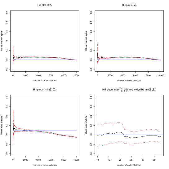
Figure 5. Exploratory plots for Example 3.2, Case 2, with α=0.5,α=1,α0=1.25formulae-sequence𝛼0.5formulae-sequencesuperscript𝛼1subscript𝛼01.25\alpha=0.5,\alpha^{*}=1,\alpha_{0}=1.25. Top panel: Hill plots for the marginals Z1subscript𝑍1Z_{1} and Z2subscript𝑍2Z_{2}. Bottom left: Hill plot for min{Z1,Z2}subscript𝑍1subscript𝑍2\min\{Z_{1},Z_{2}\}. Bottom right: Hill plot for max{Z1/Z2,Z2/Z1}subscript𝑍1subscript𝑍2subscript𝑍2subscript𝑍1\max\{Z_{1}/Z_{2},Z_{2}/Z_{1}\} thresholded by the 200 largest values of min{Z1,Z2}subscript𝑍1subscript𝑍2\min\{Z_{1},Z_{2}\}.

We generate 10000 iid samples following the construction of 𝒁=𝒀+𝑽𝒁𝒀𝑽\boldsymbol{Z}=\boldsymbol{Y}+\boldsymbol{V} described above and check whether we can estimate the regular variation index α=0.5𝛼0.5\alpha=0.5, the hidden regular variation index α+α=1.5𝛼superscript𝛼1.5\alpha+\alpha^{*}=1.5 and the tail index of G1subscript𝐺1G_{1} and G2subscript𝐺2G_{2} from the sample. Figure 4 shows Hill plots for Z1subscript𝑍1Z_{1} and Z2subscript𝑍2Z_{2} in the top panel, both of which indicate that the marginals are heavy tailed with parameter α=0.5𝛼0.5\alpha=0.5. The Hill plot of min{Z1,Z2}subscript𝑍1subscript𝑍2\min\{Z_{1},Z_{2}\} correctly identifies the HRV parameter α+α=1.5𝛼superscript𝛼1.5\alpha+\alpha^{*}=1.5. The final Hill plot of max{Z1/Z2,Z2/Z1}subscript𝑍1subscript𝑍2subscript𝑍2subscript𝑍1\max\{Z_{1}/Z_{2},Z_{2}/Z_{1}\} for the 200 highest order statistics of min{Z1,Z2}subscript𝑍1subscript𝑍2\min\{Z_{1},Z_{2}\} clearly indicates a heavy tail with a tail index of 1/2121/2 for both G1subscript𝐺1G_{1} and G2subscript𝐺2G_{2}. Note since G1=G2subscript𝐺1subscript𝐺2G_{1}=G_{2}, (1.12) allows doing the estimation using the thresholded maxima of the component ratios.

Case 2:

α+α>α0𝛼subscript𝛼subscript𝛼0\alpha+\alpha_{*}>\alpha_{0}. Let α=0.5,α=1,α0=1.25formulae-sequence𝛼0.5formulae-sequencesubscript𝛼1subscript𝛼01.25\alpha=0.5,\,\alpha_{*}=1,\,\alpha_{0}=1.25 and then α=1>0.75=α0αsubscript𝛼10.75subscript𝛼0𝛼\alpha_{*}=1>0.75=\alpha_{0}-\alpha. We generate 𝒀𝒀\boldsymbol{Y} in exactly the same way as in Case 1. For 𝑽𝑽\boldsymbol{V} we generate R𝑅R, a Pareto α0=1.25subscript𝛼01.25\alpha_{0}=1.25 random variable, B𝐵B a Bernoulli (1/2) random variable and θ𝜃\theta a Pareto α=1superscript𝛼1\alpha^{*}=1 random variable. Now define:

𝑽=BR(θ,1)+(1B)R(1,θ).𝑽𝐵𝑅𝜃11𝐵𝑅1𝜃\boldsymbol{V}=BR(\theta,1)+(1-B)R(1,\theta).

As in Case 1, 𝒁=𝒀+𝑽MRV(α=0.5,t2,ϵ{0}×ν1/2+ν1/2×ϵ{0},𝔼)𝒁𝒀𝑽MRV𝛼0.5superscript𝑡2subscriptitalic-ϵ0subscript𝜈12subscript𝜈12subscriptitalic-ϵ0𝔼\boldsymbol{Z}=\boldsymbol{Y}+\boldsymbol{V}\in\text{MRV}(\alpha=0.5,t^{2},\epsilon_{\{0\}}\times\nu_{1/2}+\nu_{1/2}\times\epsilon_{\{0\}},\mathbb{E}) and furthermore 𝒁=𝒀+𝑽MRV(α0,t1/α0,𝔼0)=MRV(1.25,t1/1.25,𝔼0)𝒁𝒀𝑽MRVsubscript𝛼0superscript𝑡1subscript𝛼0subscript𝔼0MRV1.25superscript𝑡11.25subscript𝔼0\boldsymbol{Z}=\boldsymbol{Y}+\boldsymbol{V}\in\text{MRV}(\alpha_{0},t^{1/\alpha_{0}},\mathbb{E}_{0})=\text{MRV}(1.25,t^{1/1.25},\mathbb{E}_{0}). Moreover by construction we have G1(s)=G2(s)=s1,s>1formulae-sequencesubscript𝐺1𝑠subscript𝐺2𝑠superscript𝑠1𝑠1G_{1}(s)=G_{2}(s)=s^{-1},s>1. Of course this is also clear from Proposition 3.3.

We generate 10000 iid samples using the construction of 𝒁=𝒀+𝑽𝒁𝒀𝑽\boldsymbol{Z}=\boldsymbol{Y}+\boldsymbol{V} and from this sample we estimate the regular variation index α=0.5𝛼0.5\alpha=0.5, the hidden regular variation index α0=1.25subscript𝛼01.25\alpha_{0}=1.25 and the tail index of G1subscript𝐺1G_{1} and G2subscript𝐺2G_{2} which is 111. The top panels in Figure 5 display Hill plots for Z1subscript𝑍1Z_{1} and Z2subscript𝑍2Z_{2} that indicate the same tail index of α=0.5𝛼0.5\alpha=0.5. The Hill plot for min{Z1,Z2}subscript𝑍1subscript𝑍2\min\{Z_{1},Z_{2}\} correctly indicates a tail index of α0=1.25subscript𝛼01.25\alpha_{0}=1.25. Finally, the Hill plot of max{Z1/Z2,Z2/Z1}subscript𝑍1subscript𝑍2subscript𝑍2subscript𝑍1\max\{Z_{1}/Z_{2},Z_{2}/Z_{1}\} for the 200 highest order statistics of min{Z1,Z2}subscript𝑍1subscript𝑍2\min\{Z_{1},Z_{2}\} indicates a tail index of α=1superscript𝛼1\alpha^{*}=1 for both G1G2subscript𝐺1subscript𝐺2G_{1}\equiv G_{2}.

Refer to caption
Figure 6. Exploratory plots for Example 3.2, Case 3, with α=0.5,α=1,α0=1.5formulae-sequence𝛼0.5formulae-sequencesuperscript𝛼1subscript𝛼01.5\alpha=0.5,\alpha^{*}=1,\alpha_{0}=1.5. Top panel: Hill plots for the marginals Z1subscript𝑍1Z_{1} and Z2subscript𝑍2Z_{2}. Bottom left: Hill plot for min{Z1,Z2}subscript𝑍1subscript𝑍2\min\{Z_{1},Z_{2}\}. Bottom right: Hill plot for max{Z1/Z2,Z2/Z1}subscript𝑍1subscript𝑍2subscript𝑍2subscript𝑍1\max\{Z_{1}/Z_{2},Z_{2}/Z_{1}\} thresholded by the 200 largest values of min{Z1,Z2}subscript𝑍1subscript𝑍2\min\{Z_{1},Z_{2}\}.
Case 3:

α+α=α0𝛼subscript𝛼subscript𝛼0\alpha+\alpha_{*}=\alpha_{0}. Let α=0.5,α=1,α0=1.5formulae-sequence𝛼0.5formulae-sequencesubscript𝛼1subscript𝛼01.5\alpha=0.5,\,\alpha_{*}=1,\,\alpha_{0}=1.5 which satisfies α+α=1.5=α0𝛼subscript𝛼1.5subscript𝛼0\alpha+\alpha_{*}=1.5=\alpha_{0}. We generate 𝒀𝒀\boldsymbol{Y} as in Case 1 or 2 and generate 𝑽𝑽\boldsymbol{V} using the method of Case 2, except that now R𝑅R is generated from a Pareto α0=1.5subscript𝛼01.5\alpha_{0}=1.5 distribution. We verify that 𝒁=𝒀+𝑽MRV(α=0.5,t2,ϵ{0}×ν1/2+ν1/2×ϵ{0},𝔼)𝒁𝒀𝑽MRV𝛼0.5superscript𝑡2subscriptitalic-ϵ0subscript𝜈12subscript𝜈12subscriptitalic-ϵ0𝔼\boldsymbol{Z}=\boldsymbol{Y}+\boldsymbol{V}\in\text{MRV}(\alpha=0.5,t^{2},\epsilon_{\{0\}}\times\nu_{1/2}+\nu_{1/2}\times\epsilon_{\{0\}},\mathbb{E}) and 𝒁=𝒀+𝑽MRV(1.5,t1/1.5,ν𝒁,𝔼0)𝒁𝒀𝑽MRV1.5superscript𝑡11.5subscript𝜈𝒁subscript𝔼0\boldsymbol{Z}=\boldsymbol{Y}+\boldsymbol{V}\in\text{MRV}(1.5,t^{1/1.5},\nu_{\boldsymbol{Z}},\mathbb{E}_{0}). Getting the distribution of G1subscript𝐺1G_{1} and G2subscript𝐺2G_{2} is more difficult in this case since the hidden limit measure for 𝒁𝒁\boldsymbol{Z} is more complicated as can be seen in (3.13). A careful calculation shows that G1subscript𝐺1G_{1} and G2subscript𝐺2G_{2} have regularly varying tails with index 0.50.50.5.

We generate 10000 iid samples of 𝒁=𝒀+𝑽𝒁𝒀𝑽\boldsymbol{Z}=\boldsymbol{Y}+\boldsymbol{V} using this model . In Figure 6 the Hill plots for Z1subscript𝑍1Z_{1} and Z2subscript𝑍2Z_{2} are in the neighborhood of α=0.5𝛼0.5\alpha=0.5 and the Hill plot for min{Z1,Z2}subscript𝑍1subscript𝑍2\min\{Z_{1},Z_{2}\} correctly indicates a tail index of α0=1.5subscript𝛼01.5\alpha_{0}=1.5 The Hill plot of max{Z1/Z2,Z2/Z1}subscript𝑍1subscript𝑍2subscript𝑍2subscript𝑍1\max\{Z_{1}/Z_{2},Z_{2}/Z_{1}\} for the 200 highest order statistics of min{Z1,Z2}subscript𝑍1subscript𝑍2\min\{Z_{1},Z_{2}\} indicates a tail index of α=0.5superscript𝛼0.5\alpha^{*}=0.5 for both G1G2subscript𝐺1subscript𝐺2G_{1}\equiv G_{2} which was what we were expecting.

4. Detection and estimation: regular variation and hidden regular variation

What diagnostic tools exist to help us verify that multivariate data come from a distribution possessing regular variation on some domain? Since regular variation is only an asymptotic tail property, the task of deciding to use a multivariate regularly varying model is challenging.

Suppose we have 𝒁=(Z1,Z2)𝒁subscript𝑍1subscript𝑍2\boldsymbol{Z}=(Z_{1},Z_{2}) multivariate regularly varying on 𝔼=[0,)2{𝟎}𝔼superscript020\mathbb{E}=[0,\infty)^{2}\smallsetminus\{\boldsymbol{0}\}. Under the transformation GPOLAR as defined in (1.4), 𝒁norm𝒁\|\boldsymbol{Z}\| is regularly varying with some tail index α𝛼\alpha and (1.5) holds. Diagnostics that investigate if 𝒁𝒁\boldsymbol{Z} is regularly varying often reduce the data to one dimension for instance by taking norms or max-linear combinations of 𝒁𝒁\boldsymbol{Z} [23, Chapter 8] and then apply one dimensional heavy tail diagnostics such as Hill or QQ plotting. We propose further diagnostics for the viability of a multivariate regularly varying model using the GPOLAR transformation since GPOLAR converts a regularly varying model to a conditional extreme value (CEV) model for which detection techniques exist [6].

4.1. Detecting multivariate regular variation using the CEV model

The conditional extreme value model [13, 5, 6] requires at least one of the marginals of the distribution be in the domain of attraction of an extreme value distribution. In this section we discuss a modified version of the CEV model for bivariate random vectors in the non-negative orthant where convergences are described according to the notion of 𝕄𝕄\mathbb{M}-convergence [18, 8]. Define

𝔼:=(0,)×[0,)=[0,)2([0,)×{0}).assignsubscript𝔼square-original-of00superscript0200\mathbb{E}_{\sqsupset}:=(0,\infty)\times[0,\infty)=[0,\infty)^{2}\smallsetminus\left([0,\infty)\times\{0\}\right).
Definition 4.1.

Suppose (ξ,η)+2𝜉𝜂superscriptsubscript2(\xi,\eta)\in\mathbb{R}_{+}^{2} is a random vector and there exist functions a(t),b(t)>0formulae-sequence𝑎𝑡𝑏𝑡0a(t)\to\infty,\,b(t)>0 for t>0𝑡0t>0 and a non-null measure μ𝕄(𝔼)𝜇𝕄subscript𝔼square-original-of\mu\in\mathbb{M}(\mathbb{E}_{\sqsupset}) such that in

(4.1) tP[(ξa(t),ηb(t))]μ(), in 𝕄(𝔼).𝑡𝑃delimited-[]𝜉𝑎𝑡𝜂𝑏𝑡𝜇 in 𝕄subscript𝔼square-original-of\displaystyle tP\left[\left(\frac{\xi}{{a}(t)},\frac{\eta}{{b}(t)}\right)\in\;\cdot\;\right]\to\mu(\cdot),\qquad\text{ in }\mathbb{M}(\mathbb{E}_{\sqsupset}).

Additionally assume that

  • (a)

    μ((r,]×[0,s])𝜇𝑟0𝑠\mu((r,\infty]\times[0,s]) is a non-degenerate measure in s[0,)𝑠0s\in[0,\infty) for any fixed r>0𝑟0r>0, and,

  • (b)

    H(s):=μ((1,×[0,s]))assign𝐻𝑠𝜇10𝑠H(s):=\mu((1,\infty\times[0,s])) is a probability distribution.

Then we say (ξ,η)𝜉𝜂(\xi,\eta) satisfies a conditional extreme value model and write (ξ,η)CEV(a,b,μ)𝜉𝜂CEV𝑎𝑏𝜇(\xi,\eta)\in\text{CEV}({a,b},\mu).

Remark 4.1.

The definition has some consequences [13, Section 2]:

  1. (1)

    Convergence in (4.1) implies that ξ𝜉\xi is regularly varying with some tail index α>0𝛼0\alpha>0. Consequently a(t)RV1/α𝑎𝑡𝑅subscript𝑉1𝛼a(t)\in RV_{1/\alpha}.

  2. (2)

    The limit μ𝜇\mu is a product measure of the form

    μ((r,)×[0,s])=rαH(s)=:να(r,)H(s)\mu((r,\infty)\times[0,s])=r^{-\alpha}H(s)=:\nu_{\alpha}(r,\infty)H(s)

    for all (r,s)𝔼𝑟𝑠subscript𝔼square-original-of(r,s)\in\mathbb{E}_{\sqsupset} if and only if

    limtb(tc)b(t)=1.subscript𝑡𝑏𝑡𝑐𝑏𝑡1\lim_{t\to\infty}\frac{b(tc)}{b(t)}=1.
  3. (3)

    If a(t)=b(t),t>0formulae-sequence𝑎𝑡𝑏𝑡𝑡0a(t)=b(t),t>0 then (ξ,η)𝜉𝜂(\xi,\eta) is multivariate regularly varying on 𝔼subscript𝔼square-original-of\mathbb{E}_{\sqsupset} with limit measure μ𝜇\mu. (In such a case μ𝜇\mu cannot be a product measure).

Remark 4.2.

Statistical plots that check whether bivariate data can be modelled by a CEV model were derived in [5] and are based on the Hillish, Pickandsish and Kendall’s Tau statistics. If data is generated from a CEV model, these statistics tend to a constant as the sample size increases. We concentrate on the Hillish and Pickandsish statistics for this paper. We will further specialize to the case where μ𝜇\mu is a product measure μ=να×H𝜇subscript𝜈𝛼𝐻\mu=\nu_{\alpha}\times H for reasons that will be clear in the next subsection.

Suppose (ξi,ηi);1insubscript𝜉𝑖subscript𝜂𝑖1𝑖𝑛(\xi_{i},\eta_{i});1\leqslant i\leqslant n are iid samples in +2subscriptsuperscript2\mathbb{R}^{2}_{+} and (ξ1,η1)CEV(a,b,μ)subscript𝜉1subscript𝜂1CEV𝑎𝑏𝜇(\xi_{1},\eta_{1})\in\text{CEV}(a,b,\mu) for some a(t),b(t)>0formulae-sequence𝑎𝑡𝑏𝑡0a(t)\to\infty,b(t)>0 and μ𝕄(𝔼)𝜇𝕄subscript𝔼square-original-of\mu\in\mathbb{M}(\mathbb{E}_{\sqsupset}). We use the following notation:

ξ(1)ξ(n)The decreasing order statistics of ξ1,,ξn.ηi,1inThe η-variable corresponding to ξ(i), also called the concomitant of ξ(i).Nik=l=ik𝟏{ηlηi}Rank of ηi among η1,,ηk. We write Ni=Nik.η1:kη2:kηk:kThe increasing order statistics of η1,,ηk.subscript𝜉1subscript𝜉𝑛The decreasing order statistics of ξ1,,ξn.missing-subexpressionmissing-subexpressionsuperscriptsubscript𝜂𝑖1𝑖𝑛The η-variable corresponding to ξ(i), also calledmissing-subexpressionmissing-subexpressionmissing-subexpression the concomitant of ξ(i).missing-subexpressionmissing-subexpressionsuperscriptsubscript𝑁𝑖𝑘superscriptsubscript𝑙𝑖𝑘subscript1superscriptsubscript𝜂𝑙superscriptsubscript𝜂𝑖Rank of ηi among η1,,ηk. We write Ni=Nik.missing-subexpressionmissing-subexpressionsuperscriptsubscript𝜂:1𝑘superscriptsubscript𝜂:2𝑘superscriptsubscript𝜂:𝑘𝑘The increasing order statistics of η1,,ηk.missing-subexpressionmissing-subexpression\begin{array}[]{llll}\xi_{(1)}\geqslant\ldots\geqslant\xi_{(n)}&\text{The decreasing order statistics of $\xi_{1},\ldots,\xi_{n}$.}\\[5.69054pt] \eta_{i}^{*},~{}1\leqslant i\leqslant n&\text{The $\eta$-variable corresponding to $\xi_{(i)}$, also called}\\[5.69054pt] &\text{ the concomitant of $\xi_{(i)}$.}\\[5.69054pt] N_{i}^{k}=\sum\limits_{l=i}^{k}\boldsymbol{1}_{\{\eta_{l}^{*}\leqslant\eta_{i}^{*}\}}&\text{Rank of $\eta^{*}_{i}$ among $\eta_{1}^{*},\ldots,\eta_{k}^{*}$. We write $N_{i}=N_{i}^{k}$.}\\[5.69054pt] \eta_{1:k}^{*}\leqslant\eta_{2:k}^{*}\leqslant\ldots\leqslant\eta_{k:k}^{*}&\text{The increasing order statistics of $\eta_{1}^{*},\ldots,\eta_{k}^{*}$.}\\[8.53581pt] \end{array}

Hillish statistic. For 1kn1𝑘𝑛1\leqslant k\leqslant n, the Hillish statistic is

(4.2) Hillishk,n=Hillishk,n(ξ,η):=1kj=1klogkjlogkNjksubscriptHillish𝑘𝑛subscriptHillish𝑘𝑛𝜉𝜂assign1𝑘superscriptsubscript𝑗1𝑘𝑘𝑗𝑘superscriptsubscript𝑁𝑗𝑘\displaystyle\text{Hillish}_{k,n}=\text{Hillish}_{k,n}(\mathbb{\xi},\mathbb{\eta}):=\frac{1}{k}\sum\limits_{j=1}^{k}\log\frac{k}{j}\log\frac{k}{N_{j}^{k}}
Proposition 4.1 (Proposition 2.2 and Proposition 2.3 [6]).

Suppose (ξi,ηi);subscript𝜉𝑖subscript𝜂𝑖(\xi_{i},\eta_{i}); 1in1𝑖𝑛1\leqslant i\leqslant n are iid observations from the CEV(a,b,μ)CEV𝑎𝑏𝜇\text{CEV}(a,b,\mu) model as in Definition 4.1 and suppose H𝐻H is continuous. If k=k(n),nformulae-sequence𝑘𝑘𝑛𝑛k=k(n)\to\infty,\,n\to\infty and k/n0𝑘𝑛0k/n\to 0, then

(4.3) Hillishk,nP11μ((r1α,)×[0,H(s1)])drrdss=:Iμ.\displaystyle\text{Hillish}_{k,n}\stackrel{{\scriptstyle\lower 0.60275pt\hbox{$\scriptscriptstyle\it{P}$}}}{{\rightarrow}}\int\limits_{1}^{\infty}\int\limits_{1}^{\infty}\mu((r^{\frac{1}{\alpha}},\infty)\times[0,H^{\leftarrow}(s^{-1})])\frac{dr}{r}\frac{ds}{s}=:I_{\mu}.

Moreover μ𝜇\mu is a product measure if and only if both

Hillishk,n(ξ,η)P1andHillishk,n(ξ,η)P1.formulae-sequencesuperscript𝑃subscriptHillish𝑘𝑛𝜉𝜂1andsuperscript𝑃subscriptHillish𝑘𝑛𝜉𝜂1\displaystyle\text{Hillish}_{k,n}(\mathbb{\xi},\mathbb{\eta})\stackrel{{\scriptstyle\lower 0.60275pt\hbox{$\scriptscriptstyle\it{P}$}}}{{\rightarrow}}1\quad\text{and}\quad\text{Hillish}_{k,n}(\mathbb{\xi},-\mathbb{\eta})\stackrel{{\scriptstyle\lower 0.60275pt\hbox{$\scriptscriptstyle\it{P}$}}}{{\rightarrow}}1.

Proof. The proof follows from Propositions 2.2 and 2.3 in [6]. The only difference here is the use of measure μ𝜇\mu instead of μsuperscript𝜇\mu^{*} and the roles of the first and the second components are switched.

Pickandsish statistic. This statistic gives another way to check the suitability of the CEV assumption and to detect a product measure in the limit. The Pickandsish statistic is based on ratios of differences of ordered concomitants and is patterned on the Pickands estimate for the scale parameter of an extreme value distribution (Pickands [20], de Haan and Ferreira [9, page 83], Resnick [23, page 93]). For notational convenience for st𝑠𝑡s\leqslant t write ηs:t:=ηs:tassignsubscriptsuperscript𝜂:𝑠𝑡subscriptsuperscript𝜂:𝑠𝑡\eta^{*}_{s:t}:=\eta^{*}_{\lceil s\rceil:\lceil t\rceil}. We define the Pickandsish statistic for 0<q<10𝑞10<q<1 as

(4.4) Pickandsishk,n(q):=ηqk:kηqk/2:k/2ηqk:kηqk/2:k.assignsubscriptPickandsish𝑘𝑛𝑞superscriptsubscript𝜂:𝑞𝑘𝑘superscriptsubscript𝜂:𝑞𝑘2𝑘2superscriptsubscript𝜂:𝑞𝑘𝑘superscriptsubscript𝜂:𝑞𝑘2𝑘\displaystyle\text{Pickandsish}_{k,n}(q):=\frac{\eta_{qk:k}^{*}-\eta_{qk/2:k/2}^{*}}{\eta_{qk:k}^{*}-\eta_{qk/2:k}^{*}}.
Proposition 4.2 (Proposition 2.4 and Corollary 2.5 [6]).

Suppose (ξi,ηi);subscript𝜉𝑖subscript𝜂𝑖(\xi_{i},\eta_{i}); 1in1𝑖𝑛1\leqslant i\leqslant n are iid observations from the CEV(a,b,μ)CEV𝑎𝑏𝜇\text{CEV}(a,b,\mu) model as in Definition 4.1. Assume that k=k(n),nformulae-sequence𝑘𝑘𝑛𝑛k=k(n)\to\infty,\,n\to\infty and k/n0𝑘𝑛0k/n\to 0. Then

(4.5) Pickandsishk,n(q)subscriptPickandsish𝑘𝑛𝑞\displaystyle\text{Pickandsish}_{k,n}(q) PH(q)(12ρ)H(q)H(q/2),superscript𝑃absentsuperscript𝐻𝑞1superscript2𝜌superscript𝐻𝑞superscript𝐻𝑞2\displaystyle\stackrel{{\scriptstyle\lower 0.60275pt\hbox{$\scriptscriptstyle\it{P}$}}}{{\rightarrow}}\frac{H^{\leftarrow}(q)(1-2^{\rho})}{H^{\leftarrow}(q)-H^{\leftarrow}(q/2)},

provided H(q)H(q/2)0superscript𝐻𝑞superscript𝐻𝑞20H^{\leftarrow}(q)-H^{\leftarrow}(q/2)\neq 0. Here ρ=(log(c))1log(limtb(tc)b(t))𝜌superscript𝑐1subscript𝑡𝑏𝑡𝑐𝑏𝑡\rho=(\log(c))^{-1}\log\left(\lim\limits_{t\to\infty}\frac{b(tc)}{b(t)}\right). Moreover, μ𝜇\mu is a product measure if and only if

Pickandsishk,n(q)P0superscript𝑃subscriptPickandsish𝑘𝑛𝑞0\text{Pickandsish}_{k,n}(q)\stackrel{{\scriptstyle\lower 0.60275pt\hbox{$\scriptscriptstyle\it{P}$}}}{{\rightarrow}}0

for some 0<q<10𝑞10<q<1 where H(q)H(q/2)0superscript𝐻𝑞superscript𝐻𝑞20H^{\leftarrow}(q)-H^{\leftarrow}(q/2)\neq 0.

Proof. The proof follows from Proposition 2.4 in [6]. The second part is immediate from (4.5).

4.2. Relating MRV and CEV

We have methods to detect a CEV model and indicate when the limit is a product measure. What is the connection with multivariate regular variation? This connection is given in (1.6)–(1.9). Regular variation of a vector 𝒁𝒁\boldsymbol{Z} on 𝔼𝔼\mathbb{E} and 𝔼0subscript𝔼0\mathbb{E}_{0} with scaling functions b(t)RV1/α𝑏𝑡𝑅subscript𝑉1𝛼b(t)\in RV_{1/\alpha} and b0(t)RV1/α0subscript𝑏0𝑡𝑅subscript𝑉1subscript𝛼0b_{0}(t)\in RV_{1/\alpha_{0}} respectively with 0<αα00𝛼subscript𝛼00<\alpha\leqslant\alpha_{0} is equivalent to:

(4.6) tP[(𝒁/b(t),𝒁/𝒁)]να×S(), in 𝕄((0,)×𝟎)𝑡𝑃delimited-[]norm𝒁𝑏𝑡𝒁norm𝒁subscript𝜈𝛼𝑆 in 𝕄0subscript0\displaystyle tP\bigl{[}\bigl{(}\|\boldsymbol{Z}\|/b(t),\boldsymbol{Z}/\|\boldsymbol{Z}\|\bigr{)}\in\cdot\,\bigr{]}\to\nu_{\alpha}\times S(\cdot),\quad\text{ in }\mathbb{M}((0,\infty)\times\aleph_{\boldsymbol{0}})
and
(4.7) tP[(Z1Z2b0(t),𝒁Z1Z2)]να0×S0() in 𝕄((0,)×[axes]).𝑡𝑃delimited-[]subscript𝑍1subscript𝑍2subscript𝑏0𝑡𝒁subscript𝑍1subscript𝑍2subscript𝜈subscript𝛼0subscript𝑆0 in 𝕄0subscriptdelimited-[]axes\displaystyle tP\Bigl{[}\Bigl{(}\frac{Z_{1}\wedge Z_{2}}{b_{0}(t)},\frac{\boldsymbol{Z}}{Z_{1}\wedge Z_{2}}\Bigr{)}\in\cdot\Bigr{]}\to\nu_{\alpha_{0}}\times S_{0}(\cdot)\qquad\text{ in }\mathbb{M}\bigl{(}(0,\infty)\times\aleph_{[\text{axes}]}).

If 𝟎subscript0\aleph_{\boldsymbol{0}} and [axes]subscriptdelimited-[]axes\aleph_{[\text{axes}]} were subsets of [0,)0[0,\infty) we could conclude that (4.6) and (4.7) describe CEV models and modest changes, described in the next two results, allow use of the CEV model diagnostics.

Proposition 4.3.

Suppose 𝐙𝐙\boldsymbol{Z} is a random element of +2.superscriptsubscript2\mathbb{R}_{+}^{2}. Fix a norm for 𝐳+2:(z1,z2)=z1+z2:𝐳superscriptsubscript2normsubscript𝑧1subscript𝑧2subscript𝑧1subscript𝑧2\boldsymbol{z}\in\mathbb{R}_{+}^{2}:\|(z_{1},z_{2})\|=z_{1}+z_{2}. Then 𝐙MRV(α,b(t),ν,𝔼)𝐙MRV𝛼𝑏𝑡𝜈𝔼\boldsymbol{Z}\in\text{MRV}(\alpha,b(t),\nu,\mathbb{E}) (which means (1.8) also holds) if and only if (Z,Z1Z)CEV(b,1,μ)norm𝑍subscript𝑍1norm𝑍𝐶𝐸𝑉𝑏1𝜇\left(\|Z\|,\frac{Z_{1}}{\|Z\|}\right)\in CEV(b,1,\mu) with limit measure μ=να×S¯𝜇subscript𝜈𝛼¯𝑆\mu=\nu_{\alpha}\times\bar{S} where S¯(A)=S((x,y)𝟎:xA)\bar{S}(A)=S((x,y)\in\aleph_{\boldsymbol{0}}:x\in A) for any A[0,)𝐴0A\in\mathcal{B}[0,\infty).

Proof. The proof is easily deducible from the relationship between S𝑆S and S¯¯𝑆\bar{S}.

Proposition 4.4.

Suppose 𝐙0𝐙0\boldsymbol{Z}\geqslant 0 is regularly varying on 𝔼𝔼\mathbb{E} with function b(t)RV1/α𝑏𝑡𝑅subscript𝑉1𝛼b(t)\in RV_{1/\alpha}. Then 𝐙𝐙\boldsymbol{Z} exhibits HRV on 𝔼0subscript𝔼0\mathbb{E}_{0} with scaling function b0(t)RV1/α0,α0αformulae-sequencesubscript𝑏0𝑡𝑅subscript𝑉1subscript𝛼0subscript𝛼0𝛼b_{0}(t)\in RV_{1/\alpha_{0}},\alpha_{0}\geqslant\alpha if and only if

(Z1Z2,(Z1Z2Z2Z1))CEV(b0,1,μ0)subscript𝑍1subscript𝑍2subscript𝑍1subscript𝑍2subscript𝑍2subscript𝑍1CEVsubscript𝑏01subscript𝜇0\left(Z_{1}\wedge Z_{2},\left(\frac{Z_{1}}{Z_{2}}\bigvee\frac{Z_{2}}{Z_{1}}\right)\right)\in\text{CEV}(b_{0},1,\mu_{0})

with limit measure given by μ0=να0×(pG1+(1p)G2)subscript𝜇0subscript𝜈subscript𝛼0𝑝subscript𝐺11𝑝subscript𝐺2\mu_{0}=\nu_{\alpha_{0}}\times\left(pG_{1}+(1-p)G_{2}\right) where G1(s)=S0([1,s]×{1})subscript𝐺1𝑠subscript𝑆01𝑠1G_{1}(s)=S_{0}([1,s]\times\{1\}) and G2(s)=S0({1}×[1,s])subscript𝐺2𝑠subscript𝑆011𝑠G_{2}(s)=S_{0}(\{1\}\times[1,s]) for s1𝑠1s\geqslant 1 and G1(s)=G2(s)=0,s1.formulae-sequencesubscript𝐺1𝑠subscript𝐺2𝑠0𝑠1G_{1}(s)=G_{2}(s)=0,s\leqslant 1.

Proof.

The proof follows from the connection between S0subscript𝑆0S_{0} and G1,G2subscript𝐺1subscript𝐺2G_{1},G_{2}. ∎

5. Testing for MRV and HRV: data examples

Here we analyze data sets to see whether a multivariate regularly varying model is a valid assumption. We also look for asymptotic independence and if it exists we test for the existence of hidden regular variation.

Example 5.1.

Boston University: HTTP downloads.
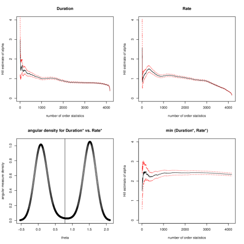
Refer to caption
Figure 7. BU dataset. Top panel: Hill plots of tail parameters for D𝐷D and R𝑅R. Bottom left plot: angular density of (D,R)superscript𝐷superscript𝑅(D^{*},R^{*}). Bottom right plot: Hill plot for min(D,R)superscript𝐷superscript𝑅\min(D^{*},R^{*}).

The first data set is obtained from a now classical Boston University study [3] which suggested self-similarity and heavy tails in web-traffic data. Our dataset was created from HTTP downloads in sessions initiated by logins at a Boston University computer laboratory. It consists of 8 hours 20 minutes worth of downloads in February 1995 after applying an aggregation rule to downloads to associate machine triggered actions with human requests and is discussed in [12, page 176]. The result of the aggregation is 4161 downloads which are characterized by the following variables:

  • S=𝑆absentS= the size of the download in kilobytes,

  • D=𝐷absentD= the duration of the download in seconds,

  • R=𝑅absentR= throughput of the download; that is, =S/Dabsent𝑆𝐷=S/D.

Previous studies [23, page 299, 316] indicate heavy tailed behavior of all three variables and asymptotic independence between D𝐷D and R𝑅R. We concentrate on the variables (D,R)𝐷𝑅(D,R) so our data is {(Di,Ri);1i4161}subscript𝐷𝑖subscript𝑅𝑖1𝑖4161\{(D_{i},R_{i});1\leqslant i\leqslant 4161\}. Moreover the rank-transformed variables are denoted:

Disuperscriptsubscript𝐷𝑖\displaystyle D_{i}^{*} =j=14161𝟏{DiDj},absentsuperscriptsubscript𝑗14161subscript1subscript𝐷𝑖subscript𝐷𝑗\displaystyle=\sum_{j=1}^{4161}\boldsymbol{1}_{\{D_{i}\geqslant D_{j}\}}, Ri=j=14161𝟏{RiRj}.superscriptsubscript𝑅𝑖superscriptsubscript𝑗14161subscript1subscript𝑅𝑖subscript𝑅𝑗\displaystyle R_{i}^{*}=\sum_{j=1}^{4161}\boldsymbol{1}_{\{R_{i}\geqslant R_{j}\}}.

for 1i41611𝑖41611\leqslant i\leqslant 4161 with the generic rank-transformed variables denoted Dsuperscript𝐷D^{*} and Rsuperscript𝑅R^{*} respectively.

Refer to caption
Figure 8. BU dataset. Top panel (D>Rsuperscript𝐷superscript𝑅D^{*}>R^{*}): Hillish plots for (A,θ1)𝐴subscript𝜃1(A,\theta_{1}) and (A,θ1)𝐴subscript𝜃1(A,-\theta_{1}) and Pickandsish plot for (A,θ1)𝐴subscript𝜃1(A,\theta_{1}) at q=0.8𝑞0.8q=0.8. Bottom panel (D<Rsuperscript𝐷superscript𝑅D^{*}<R^{*}): Hillish plots for (A,θ2)𝐴subscript𝜃2(A,\theta_{2}) and (A,θ2)𝐴subscript𝜃2(A,-\theta_{2}) and Pickandsish plot for (A,θ2)𝐴subscript𝜃2(A,\theta_{2}) at q=0.8𝑞0.8q=0.8.

In Figure 7 we plot Hill estimates of the tail parameters of D𝐷D and R𝑅R for increasing number of order statistics of their respective univariate data values. Both plots are consistent with D𝐷D and R𝑅R being heavy tailed with tail parameters αDsubscript𝛼𝐷\alpha_{D} and αRsubscript𝛼𝑅\alpha_{R} greater than 1. (This is confirmed [23, 10, 25] by altHill and QQ plots–not shown–showing α^D=1.4subscript^𝛼𝐷1.4\hat{\alpha}_{D}=1.4 and α^R=1.2subscript^𝛼𝑅1.2\hat{\alpha}_{R}=1.2.) The angular density plot of (D,R)superscript𝐷superscript𝑅(D^{*},R^{*}) shows data concentration near 00 and π/2𝜋2\pi/2 consistent with asymptotic independence of the quantities. Asymptotic independence does not automatically imply HRV so we check for HRV on 𝔼0subscript𝔼0\mathbb{E}_{0}.

Refer to caption
Figure 9. BU dataset. Proportion of data with Di>Risuperscriptsubscript𝐷𝑖superscriptsubscript𝑅𝑖D_{i}^{*}>R_{i}^{*} for order statistics of Ai=min{Di,Ri}subscript𝐴𝑖superscriptsubscript𝐷𝑖superscriptsubscript𝑅𝑖A_{i}=\min\{D_{i}^{*},R_{i}^{*}\}.
Refer to caption
Figure 10. BU dataset. Top panel: QQ plot of log(D/R)superscript𝐷superscript𝑅\log(D^{*}/R^{*}) when Ai>A(100)subscript𝐴𝑖subscript𝐴100A_{i}>A_{(100)} and Hill plots of D/Rsuperscript𝐷superscript𝑅D^{*}/R^{*} when Ai>A(100)subscript𝐴𝑖subscript𝐴100A_{i}>A_{(100)} and Ai>A(400)subscript𝐴𝑖subscript𝐴400A_{i}>A_{(400)}. Bottom panel: Histogram of D/Rsuperscript𝐷superscript𝑅D^{*}/R^{*} when Ai>A(100)subscript𝐴𝑖subscript𝐴100A_{i}>A_{(100)} and kernel density estimates of D/Rsuperscript𝐷superscript𝑅D^{*}/R^{*} when Ai>A(100)subscript𝐴𝑖subscript𝐴100A_{i}>A_{(100)} and Ai>A(400)subscript𝐴𝑖subscript𝐴400A_{i}>A_{(400)}.
Refer to caption
Figure 11. BU dataset. Top panel: QQ plot of log(R/D)superscript𝑅superscript𝐷\log(R^{*}/D^{*}) when Ai>A(100)subscript𝐴𝑖subscript𝐴100A_{i}>A_{(100)} along with Hill plots of R/Dsuperscript𝑅superscript𝐷R^{*}/D^{*} when Ai>A(100)subscript𝐴𝑖subscript𝐴100A_{i}>A_{(100)} and Ai>A(400)subscript𝐴𝑖subscript𝐴400A_{i}>A_{(400)}. Bottom panel: Histogram of R/Dsuperscript𝑅superscript𝐷R^{*}/D^{*} when Ai>A(100)subscript𝐴𝑖subscript𝐴100A_{i}>A_{(100)} and kernel density estimates of R/Dsuperscript𝑅superscript𝐷R^{*}/D^{*} when Ai>A(100)subscript𝐴𝑖subscript𝐴100A_{i}>A_{(100)} and Ai>A(400).subscript𝐴𝑖subscript𝐴400A_{i}>A_{(400)}.

The rank transformation causes (D,R)superscript𝐷superscript𝑅(D^{*},R^{*}) to be standard regularly varying with α=1𝛼1\alpha=1 and Proposition 4.4 implies (D,R)superscript𝐷superscript𝑅(D^{*},R^{*}) has hidden regular variation on 𝔼0subscript𝔼0\mathbb{E}_{0} if (and only if)

(A,θ):=(min{D,R},max{DR,RD})CEV(b0,1,μ0)assign𝐴𝜃superscript𝐷superscript𝑅superscript𝐷superscript𝑅superscript𝑅superscript𝐷CEVsubscript𝑏01subscript𝜇0(A,\theta):=\left(\min\{D^{*},R^{*}\},\max\left\{\frac{D^{*}}{R^{*}},\frac{R^{*}}{D^{*}}\right\}\right)\in\text{CEV}(b_{0},1,\mu_{0})

for some function b0subscript𝑏0b_{0}. We proceed by testing the following:

  1. (1)

    Is the variable A=min{D,R}𝐴superscript𝐷superscript𝑅A=\min\{D^{*},R^{*}\} regularly varying with parameter greater than 1? The bottom right plot in Figure 7 plots Hill estimates for increasing number of order statistics of A𝐴A and stabilizes between 2 and 3 indicating the desired heavy tail behavior.

  2. (2)

    For D>Rsuperscript𝐷superscript𝑅D^{*}>R^{*}, we check whether (A,θ1):=(min{D,R},DR)assign𝐴subscript𝜃1superscript𝐷superscript𝑅superscript𝐷superscript𝑅(A,\theta_{1}):=(\min\{D^{*},R^{*}\},\frac{D^{*}}{R^{*}}) follows a CEV model. In the top panel of Figure 8, the Hillish plots of (A,θ1)𝐴subscript𝜃1(A,\theta_{1}) and (A,θ1)𝐴subscript𝜃1(A,-\theta_{1}) are close to 1 near the left side of their plots. Moreover we observe that the Pickandsish estimate at q=0.8𝑞0.8q=0.8 also remains near 0. From Propositions 4.1 and 4.2, this is consistent with (A,θ1)CEV(b0,1,μ0)𝐴subscript𝜃1CEVsubscript𝑏01subscript𝜇0(A,\theta_{1})\in\text{CEV}(b_{0},1,\mu_{0}) with a limit measure of the CEV being a product measure.

  3. (3)

    For D<Rsuperscript𝐷superscript𝑅D^{*}<R^{*}, we similarly check whether (A,θ2):=(min{R,D},RD)assign𝐴subscript𝜃2superscript𝑅superscript𝐷superscript𝑅superscript𝐷(A,\theta_{2}):=(\min\{R^{*},D^{*}\},\frac{R^{*}}{D^{*}}) follows a CEV model. In the bottom panel of Figure 8 we observe that the Hillish plots of (A,θ2)𝐴subscript𝜃2(A,\theta_{2}) and (A,θ2)𝐴subscript𝜃2(A,-\theta_{2}) are close to 1 near the left side of their plots. We also observe that the Pickandsish estimate at q=0.8𝑞0.8q=0.8 remains near 0. Hence we again conclude that the evidence is consistent with (A,θ2)CEV(b0,1,μ0)𝐴subscript𝜃2CEVsubscript𝑏01subscript𝜇0(A,\theta_{2})\in\text{CEV}(b_{0},1,\mu_{0}) with a limit measure of the CEV being a product measure.

Thus modeling the joint distribution of (D,R)𝐷𝑅(D,R) using MRV and HRV is consistent with the data. The next step is to estimate the distributions of θ1G1similar-tosubscript𝜃1subscript𝐺1\theta_{1}\sim G_{1} and θ2G2similar-tosubscript𝜃2subscript𝐺2\theta_{2}\sim G_{2} as well as q𝑞q defined in Proposition 4.4. Figure 9 plots q^k=1ki=14161𝟏{Di>Ri,Ai>A(k)},k=2,,4161,formulae-sequencesubscript^𝑞𝑘1𝑘superscriptsubscript𝑖14161subscript1formulae-sequencesuperscriptsubscript𝐷𝑖superscriptsubscript𝑅𝑖subscript𝐴𝑖subscript𝐴𝑘𝑘24161\hat{q}_{k}=\frac{1}{k}\sum_{i=1}^{4161}\boldsymbol{1}_{\{D_{i}^{*}>R_{i}^{*},A_{i}>A_{(k)}\}},\quad k=2,\ldots,4161, where Ai=min{Ri,Di}subscript𝐴𝑖subscriptsuperscript𝑅𝑖subscriptsuperscript𝐷𝑖A_{i}=\min\{R^{*}_{i},D^{*}_{i}\} and A(1)A(2)subscript𝐴1subscript𝐴2A_{(1)}\geqslant A_{(2)}\geqslant\ldots form order statistics from Ai;1i4161subscript𝐴𝑖1𝑖4161A_{i};1\leqslant i\leqslant 4161. Observing Figure 9 for k𝑘k near 0, an estimate of q𝑞q is q^=0.6^𝑞0.6\hat{q}=0.6.

To find the distribution of θ1subscript𝜃1\theta_{1} we make a standard exponential QQ plot of log(Di/Ri)subscriptsuperscript𝐷𝑖subscriptsuperscript𝑅𝑖\log(D^{*}_{i}/R^{*}_{i}) where Ai=min(Di,Ri)>A(100)subscript𝐴𝑖subscriptsuperscript𝐷𝑖subscriptsuperscript𝑅𝑖subscript𝐴100A_{i}=\min(D^{*}_{i},R^{*}_{i})>A_{(100)}, which serves as an exploratory diagnostic for heavy tails. We also create Hill plots for Di/Risubscriptsuperscript𝐷𝑖subscriptsuperscript𝑅𝑖D^{*}_{i}/R^{*}_{i} where Ai>A(k)subscript𝐴𝑖subscript𝐴𝑘A_{i}>A_{(k)} for two choices of k𝑘k. The top panels of Figure 10 give the QQ plot for k=100𝑘100k=100 (left) and the Hill plots for k=100𝑘100k=100 and 400400400 (middle and right). The bottom panels in Figure 10 have a histogram of Di/Risuperscriptsubscript𝐷𝑖superscriptsubscript𝑅𝑖D_{i}^{*}/R_{i}^{*} for Ai>A(100)subscript𝐴𝑖subscript𝐴100A_{i}>A_{(100)} (left) and kernel density plots of Di/Risuperscriptsubscript𝐷𝑖superscriptsubscript𝑅𝑖D_{i}^{*}/R_{i}^{*} for Ai>A(100)subscript𝐴𝑖subscript𝐴100A_{i}>A_{(100)} (middle) and Ai>A(100)subscript𝐴𝑖subscript𝐴100A_{i}>A_{(100)} (right). The plots indicate G1subscript𝐺1G_{1} is heavy tailed with an index between 1.5 and 2 and we can provide a density estimate for the distribution of θ1subscript𝜃1\theta_{1}.

We create the same set of plots for finding G2subscript𝐺2G_{2} in Figure 11 which also indicates towards a similar conclusion of heavy tailed behavior for G2subscript𝐺2G_{2} with an index close to but less than 222.

Example 5.2.

UNC Chapel Hill HTTP response data.
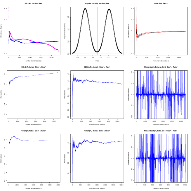
Refer to caption
Figure 12. UNC HTTP responses dataset. Top panel: (Left:) Hill plots of tail parameters for S𝑆S(blue), R𝑅R(magenta); (Middle:) angular density of (S,R)superscript𝑆superscript𝑅(S^{*},R^{*}); (Right:) Hill plot for min(S,R))\min(S^{*},R^{*})). Middle panel (S>Rsuperscript𝑆superscript𝑅S^{*}>R^{*}): Hillish plots for (A,θ1)𝐴subscript𝜃1(A,\theta_{1}) and (A,θ1)𝐴subscript𝜃1(A,-\theta_{1}) and Pickandsish plot for (A,θ1)𝐴subscript𝜃1(A,\theta_{1}) at q=0.8𝑞0.8q=0.8. Bottom panel (S<Rsuperscript𝑆superscript𝑅S^{*}<R^{*}): Hillish plots for (A,θ2)𝐴subscript𝜃2(A,\theta_{2}) and (A,θ2)𝐴subscript𝜃2(A,-\theta_{2}) and Pickandsish plot for (A,θ2)𝐴subscript𝜃2(A,\theta_{2}) at q=0.8𝑞0.8q=0.8.

A response is the data transfer resulting from an HTTP request. The data set [14] consists of 21,828 thresholded responses bigger than 100 kilobytes measured between 1:00pm and 5:00pm on 25th April, 2001. We use similar notation as in Example 5.1.

  • S=𝑆absentS= HTTP response size; total size of packets transferred in kilobytes,

  • D=𝐷absentD= the elapsed duration between first and last packets in seconds of the response,

  • R=𝑅absentR= throughput of the response =S/Dabsent𝑆𝐷=S/D.

    Refer to caption
    Figure 13. UNC HTTP responses. Proportion of data with Si>Risuperscriptsubscript𝑆𝑖superscriptsubscript𝑅𝑖S_{i}^{*}>R_{i}^{*} for order statistics of Ai=min{Si,Ri}subscript𝐴𝑖superscriptsubscript𝑆𝑖superscriptsubscript𝑅𝑖A_{i}=\min\{S_{i}^{*},R_{i}^{*}\}.

Thus, the data set consists of {(Si,Di,Ri);1i21828}subscript𝑆𝑖subscript𝐷𝑖subscript𝑅𝑖1𝑖21828\{(S_{i},D_{i},R_{i});1\leqslant i\leqslant 21828\}. Our interest is in the variables (S,R)𝑆𝑅(S,R) which exhibit heavy tails and asymptotic independence [14]. Denote the rank-transformed variables:

(Si=j=121828𝟏{SiSj},Ri=j=121828𝟏{RiRj}),1i21828,formulae-sequencesuperscriptsubscript𝑆𝑖superscriptsubscript𝑗121828subscript1subscript𝑆𝑖subscript𝑆𝑗superscriptsubscript𝑅𝑖superscriptsubscript𝑗121828subscript1subscript𝑅𝑖subscript𝑅𝑗1𝑖21828\Bigl{(}S_{i}^{*}=\sum_{j=1}^{21828}\boldsymbol{1}_{\{S_{i}\geqslant S_{j}\}},R_{i}^{*}=\sum_{j=1}^{21828}\boldsymbol{1}_{\{R_{i}\geqslant R_{j}\}}\Bigr{)},\quad 1\leqslant i\leqslant 21828,

with the generic rank-transformed variables denoted Ssuperscript𝑆S^{*} and Rsuperscript𝑅R^{*} respectively. The top left plots in Figure 12 give Hill plots of the tail indices of the distributions of S𝑆S and R𝑅R and suggest these indices are between 1 and 2. Asymptotic independence of S,R𝑆𝑅S,R is exhibited in the angular density plot (top middle plot) for (S,R)superscript𝑆superscript𝑅(S^{*},R^{*}).

We next inquire if HRV exists on 𝔼0subscript𝔼0\mathbb{E}_{0}. The Hill plot for min(S,R)superscript𝑆superscript𝑅\min(S^{*},R^{*}) on the upper right panel of Figure 12 gives a tail estimate α^0subscript^𝛼0\hat{\alpha}_{0} clearly greater than 1 and is consistent with HRV. We transform the data {(S,R); 1i21828}superscript𝑆superscript𝑅1𝑖21828\{(S^{*},R^{*});\,1\leqslant i\leqslant 21828\} with the transformation GPOLAR) to obtain:

(A,θ):=GPOLAR(S,R)=(min{S,R},max{SR,RS}).assign𝐴𝜃GPOLARsuperscript𝑆superscript𝑅superscript𝑆superscript𝑅superscript𝑆superscript𝑅superscript𝑅superscript𝑆(A,\theta):=\text{GPOLAR}(S^{*},R^{*})=\left(\min\{S^{*},R^{*}\},\max\left\{\frac{S^{*}}{R^{*}},\frac{R^{*}}{S^{*}}\right\}\right).

From Proposition 4.4 we know (A,θ)CEV(b0,1,μ0)𝐴𝜃CEVsubscript𝑏01subscript𝜇0(A,\theta)\in\text{CEV}(b_{0},1,\mu_{0}) for some function b0subscript𝑏0b_{0} and measure μ0subscript𝜇0\mu_{0} on 𝔼0subscript𝔼0\mathbb{E}_{0}. For both the cases S>Rsuperscript𝑆superscript𝑅S^{*}>R^{*} (see middle panels in Figure 12) and S<Rsuperscript𝑆superscript𝑅S^{*}<R^{*} (see bottom panels in Figure 12), we employ the Hillish and Pickandsish diagnostics to check consistency of (A,θ1):=(min{S,R},S/R)assign𝐴subscript𝜃1superscript𝑆superscript𝑅superscript𝑆superscript𝑅(A,\theta_{1}):=(\min\{S^{*},R^{*}\},{S^{*}}/{R^{*}}) and (A,θ2):=(min{S,R},R/S)assign𝐴subscript𝜃2superscript𝑆superscript𝑅superscript𝑅superscript𝑆(A,\theta_{2}):=(\min\{S^{*},R^{*}\},{R^{*}}/{S^{*}}) with the CEV model with product limit measure. The Hillish plots are reasurringly hovering at height 1 and the Pickandsish plots center at 0.
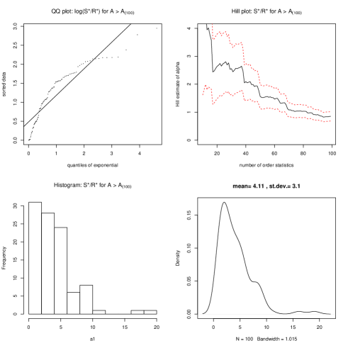
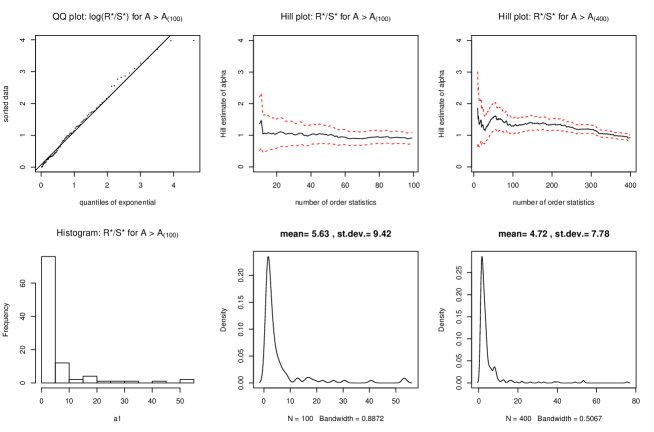
Refer to caption
Figure 14. UNC HTTP responses: Top: QQ plot of log(S/R)superscript𝑆superscript𝑅\log(S^{*}/R^{*}) when Ai>A(100)subscript𝐴𝑖subscript𝐴100A_{i}>A_{(100)} along with Hill plots of S/Rsuperscript𝑆superscript𝑅S^{*}/R^{*} when Ai>A(100)subscript𝐴𝑖subscript𝐴100A_{i}>A_{(100)} and Ai>A(400)subscript𝐴𝑖subscript𝐴400A_{i}>A_{(400)}. Bottom: Histogram and kernel density estimates of S/Rsuperscript𝑆superscript𝑅S^{*}/R^{*} when Ai>A(100)subscript𝐴𝑖subscript𝐴100A_{i}>A_{(100)}
Refer to caption
Figure 15. UNC HTTP responses. Top: QQ plot of log(R/S)superscript𝑅superscript𝑆\log(R^{*}/S^{*}) when Ai>A(100)subscript𝐴𝑖subscript𝐴100A_{i}>A_{(100)} and Hill plots of R/Ssuperscript𝑅superscript𝑆R^{*}/S^{*} when Ai>A(100)subscript𝐴𝑖subscript𝐴100A_{i}>A_{(100)} and Ai>A(400)subscript𝐴𝑖subscript𝐴400A_{i}>A_{(400)}. Bottom: Histogram of R/Ssuperscript𝑅superscript𝑆R^{*}/S^{*} when Ai>A(100)subscript𝐴𝑖subscript𝐴100A_{i}>A_{(100)} and kernel density estimates of R/Ssuperscript𝑅superscript𝑆R^{*}/S^{*} for Ai>A(100)subscript𝐴𝑖subscript𝐴100A_{i}>A_{(100)} and Ai>A(400).subscript𝐴𝑖subscript𝐴400A_{i}>A_{(400)}.

So we have accumulated evidence that the data is consistent with an HRV model on 𝔼0subscript𝔼0\mathbb{E}_{0}. Now we proceed to provide some estimates on the structure of the hidden angular measure, which boils down to estimating three things

  1. (1)

    The proportion q𝑞q appearing in μ0subscript𝜇0\mu_{0} in Proposition 4.4: this can be estimated by

    q^k=1ki=121828𝟏{Si>Ri,Ai>A(k)},k=2,,21,828.formulae-sequencesubscript^𝑞𝑘1𝑘superscriptsubscript𝑖121828subscript1formulae-sequencesuperscriptsubscript𝑆𝑖superscriptsubscript𝑅𝑖subscript𝐴𝑖subscript𝐴𝑘𝑘221828\hat{q}_{k}=\frac{1}{k}\sum_{i=1}^{21828}\boldsymbol{1}_{\{S_{i}^{*}>R_{i}^{*},A_{i}>A_{(k)}\}},\quad k=2,\ldots,21,828.

    where Ai=min{Si,Ri}subscript𝐴𝑖subscriptsuperscript𝑆𝑖subscriptsuperscript𝑅𝑖A_{i}=\min\{S^{*}_{i},R^{*}_{i}\} and A(1)A(2)subscript𝐴1subscript𝐴2A_{(1)}\geqslant A_{(2)}\geqslant\ldots form order statistics from Ai;1i21,828formulae-sequencesubscript𝐴𝑖1𝑖21828A_{i};1\leqslant i\leqslant 21,828 as in Figure 13. Looking at the plot for k𝑘k near zero, we can estimate p^=0.55^𝑝0.55\hat{p}=0.55.

  2. (2)

    The distribution of θ1G1similar-tosubscript𝜃1subscript𝐺1\theta_{1}\sim G_{1}: see Figure 14. First we make a standard exponential QQ plot of log(Si/Ri)subscriptsuperscript𝑆𝑖superscriptsubscript𝑅𝑖\log(S^{*}_{i}/R_{i}^{*}) when Ai>A(100)subscript𝐴𝑖subscript𝐴100A_{i}>A_{(100)}. This acts as a diagnostic for heavy-tails. This plot clearly indicates against heavy-tails as does a Hill plot of Si/Risubscriptsuperscript𝑆𝑖superscriptsubscript𝑅𝑖S^{*}_{i}/R_{i}^{*} when Ai>A(100)subscript𝐴𝑖subscript𝐴100A_{i}>A_{(100)}. A histogram and kernel density estimate plot of (Si/Ri)subscriptsuperscript𝑆𝑖superscriptsubscript𝑅𝑖(S^{*}_{i}/R_{i}^{*}) for Ai>A(100)subscript𝐴𝑖subscript𝐴100A_{i}>A_{(100)} points towards a light-tailed distribution.

  3. (3)

    The distribution of θ2G2similar-tosubscript𝜃2subscript𝐺2\theta_{2}\sim G_{2}: see Figure 15. As before, first we make a standard exponential QQ plot of log(Ri/Si)subscriptsuperscript𝑅𝑖superscriptsubscript𝑆𝑖\log(R^{*}_{i}/S_{i}^{*}) when Ai>A(100)subscript𝐴𝑖subscript𝐴100A_{i}>A_{(100)}, and the points nicely hug a straight line which indicates presence of heavy-tails. The Hill plots of Ri/Sisubscriptsuperscript𝑅𝑖superscriptsubscript𝑆𝑖R^{*}_{i}/S_{i}^{*} when Ai>A(100)subscript𝐴𝑖subscript𝐴100A_{i}>A_{(100)} and Ai>A(400)subscript𝐴𝑖subscript𝐴400A_{i}>A_{(400)} provide an estimate of the tail index to be between 1 and 1.5. The histograms and kernel density estimates seem to support that the distribution of G2subscript𝐺2G_{2} is heavy-tailed.

6. Conclusion

In this paper we have discussed different techniques to generate models which exhibit both regular variation and hidden regular variation. We have seen some simulated examples where we can estimate the parameters of both MRV and HRV but there are also examples where it is difficult to correctly estimate parameters. We restricted ourselves to the two dimensional non-negative orthant here, but clearly some of the generation techniques can be extended to higher dimensions. Moreover, the detection techniques for HRV on 𝔼0subscript𝔼0\mathbb{E}_{0} using the CEV model can also be extended to detect HRV on other types of cones especially in two dimensions but perhaps even more. Overall this paper serves as a starting point for methods of generating and detecting multivariate heavy tailed models having tail dependence explained by HRV.

References

  • Anderson and Meerschaert [1998] P. L. Anderson and M. M. Meerschaert. Modeling river flows with heavy tails. Water Resources Research, 34(9):2271–2280, 1998. ISSN 1944-7973. doi: 10.1029/98WR01449. URL http://dx.doi.org/10.1029/98WR01449.
  • Breiman [1965] L. Breiman. On some limit theorems similar to the arc-sin law. Theory Probab. Appl., 10:323–331, 1965.
  • Crovella and Bestavros [1996] M. Crovella and A. Bestavros. Self-similarity in world wide web traffic: evidence and possible causes. In Proceedings of the ACM SIGMETRICS ’96 International Conference on Measurement and Modeling of Computer Systems, volume 24, pages 160–169, 1996.
  • Crovella et al. [1999] M. Crovella, A. Bestavros, and M.S. Taqqu. Heavy-tailed probability distributions in the world wide web. In M.S. Taqqu R. Adler, R. Feldman, editor, A Practical Guide to Heavy Tails: Statistical Techniques for Analysing Heavy Tailed Distributions. Birkhäuser, Boston, 1999.
  • Das and Resnick [2011a] B. Das and S.I. Resnick. Conditioning on an extreme component: Model consistency with regular variation on cones. Bernoulli, 17(1):226–252, 2011a. ISSN 1350-7265. doi: 10.3150/10-BEJ271.
  • Das and Resnick [2011b] B. Das and S.I. Resnick. Detecting a conditional extreme value model. Extremes, 14(1):29–61, 2011b.
  • Das et al. [2013] B. Das, P. Embrechts, and V. Fasen. Four theorems and a financial crisis. The International Journal of Approximate Reasoning, 54(6):701–716, 2013.
  • Das et al. [2013] B. Das, A. Mitra, and S. Resnick. Living on the multi-dimensional edge: Seeking hidden risks using regular variation. Advances in Applied Probability, 45(1):139–163, 2013. ArXiv e-prints 1108.5560.
  • de Haan and Ferreira [2006] L. de Haan and A. Ferreira. Extreme Value Theory: An Introduction. Springer-Verlag, New York, 2006.
  • Drees et al. [2000] H. Drees, L. de Haan, and S.I. Resnick. How to make a Hill plot. Ann. Statist., 28(1):254–274, 2000.
  • Embrechts et al. [1997] P. Embrechts, C. Kluppelberg, and T. Mikosch. Modelling Extreme Events for Insurance and Finance. Springer-Verlag, Berlin, 1997.
  • Guerin et al. [2003] C.A. Guerin, H. Nyberg, O. Perrin, S.I. Resnick, H. Rootzén, and C. Stărică. Empirical testing of the infinite source poisson data traffic model. Stochastic Models, 19(2):151–200, 2003.
  • Heffernan and Resnick [2007] J.E. Heffernan and S.I. Resnick. Limit laws for random vectors with an extreme component. Ann. Appl. Probab., 17(2):537–571, 2007. ISSN 1050-5164. doi: 10.1214/105051606000000835.
  • Hernandez-Campos et al. [2005] F. Hernandez-Campos, K. Jeffay, C. Park, J. S. Marron, and S.I. Resnick. Extremal dependence: internet traffic applications. Stoch. Models, 21(1):1–35, 2005. ISSN 1532-6349.
  • Hult and Lindskog [2006] H. Hult and F. Lindskog. Regular variation for measures on metric spaces. Publ. Inst. Math. (Beograd) (N.S.), 80(94):121–140, 2006. ISSN 0350-1302. doi: 10.2298/PIM0694121H. URL http://dx.doi.org/10.2298/PIM0694121H.
  • Ibragimov et al. [2011] R. Ibragimov, D.. Jaffee, and J. Walden. Divesification disasters. Journal of Financial Economics, 99(2):333–348, 2011. doi: 10.1016/j.jfineco.2010.08.015.
  • Jessen and Mikosch [2006] A.H. Jessen and T. Mikosch. Regularly varying functions. Publ. Inst. Math. (Beograd) (N.S.), 80(94):171–192, 2006.
  • Lindskog et al. [2013] F. Lindskog, S.I. Resnick, and J. Roy. Regularly varying measures on metric spaces: Hidden regular variation and hidden jumps. Technical report, School of ORIE, Cornell University, 2013. URL http://arxiv.org/abs/1307.5803.
  • Maulik and Resnick [2005] K. Maulik and S.I. Resnick. Characterizations and examples of hidden regular variation. Extremes, 7(1):31–67, 2005.
  • Pickands [1975] J. Pickands. Statistical inference using extreme order statistics. Ann. Statist., 3:119–131, 1975.
  • Resnick [1986] S.I. Resnick. Point processes, regular variation and weak convergence. Adv. Applied Probability, 18:66–138, 1986.
  • Resnick [2002] S.I. Resnick. Hidden regular variation, second order regular variation and asymptotic independence. Extremes, 5(4):303–336 (2003), 2002. ISSN 1386-1999.
  • Resnick [2007] S.I. Resnick. Heavy Tail Phenomena: Probabilistic and Statistical Modeling. Springer Series in Operations Research and Financial Engineering. Springer-Verlag, New York, 2007. ISBN: 0-387-24272-4.
  • Resnick [2008] S.I. Resnick. Extreme Values, Regular Variation and Point Processes. Springer, New York, 2008. ISBN 978-0-387-75952-4. Reprint of the 1987 original.
  • Resnick and Stărică [1997] S.I. Resnick and C. Stărică. Smoothing the Hill estimator. Adv. Applied Probab., 29:271–293, 1997.
  • Smith [2003] R.L. Smith. Statistics of extremes, with applications in environment, insurance and finance. In B. Finkenstadt and H. Rootzén, editors, SemStat: Seminaire Europeen de Statistique, Exteme Values in Finance, Telecommunications, and the Environment, pages 1–78. Chapman-Hall, London, 2003.
  • Weller and Cooley [2013] G.B. Weller and D. Cooley. A sum characterization of hidden regular variation with likelihood inference via expectation-maximization. Biometrika (to appear), 2013.