Calibration and performance of the photon sensor response of FACT –
The First G-APD Cherenkov telescope

Abstract

The First G-APD Cherenkov Telescope (FACT) is the first in-operation test of the performance of silicon photo detectors in Cherenkov Astronomy. For more than two years it is operated on La Palma, Canary Islands (Spain), for the purpose of long-term monitoring of astrophysical sources. For this, the performance of the photo detectors is crucial and therefore has been studied in great detail. Special care has been taken for their temperature and voltage dependence implementing a correction method to keep their properties stable. Several measurements have been carried out to monitor the performance. The measurements and their results are shown, demonstrating the stability of the gain below the percent level. The resulting stability of the whole system is discussed, nicely demonstrating that silicon photo detectors are perfectly suited for the usage in Cherenkov telescopes, especially for long-term monitoring purpose.

1 Introduction

The First G-APD Cherenkov telescope (FACT) is the first Imaging air-Cherenkov telescope to use silicon based sensors for photo detection. Commencing operation in October 2011, the telescope is operated remotely and automatic. A complete introduction and detailed description of its hardware and software can be found in [2].

1.1 General introduction

The telescope is dedicated to the monitoring of the brightest known gamma-ray sources, mainly Active Galactic Nuclei (AGN) with their highly variable flux. Combining the observed energy spectrum with the spectral information obtained at other wavelengths (e.g. radio or X-ray data) gives an insight on cosmic particle acceleration. To understand the highly variable flaring behaviour on all time scales continuous monitoring for several months or years is necessary. Although other, much more sensitive instruments are currently available as the H.E.S.S., MAGIC and VERITAS telescopes, their high discovery potential is best used for the detection of new sources at TeV energies and precision studies of known sources. For long-term and especially continous monitoring the observation time of those instruments is too expensive which suggests the construction of an inexpensive instrument with an adapted sensitivity, c.f. [3]. In addition, the application of silicon based photo sensors promised the increase of available observation time due to their robustness against light exposure as string moon light.

The presented study is one of the first long-term tests of these sensors under real environmental conditions. The Imaging Air-Cherenkov Technique is an indirect measurement method where Cherenkov light flashes emitted by atmospheric particle cascades induced from cosmic ray particles are imaged. The camera comprises 1440 photo sensors each read out individually. As photo sensors, Geiger-mode avalanche photo diodes (G-APDs) are used. These silicon based devices are fast and sensitive photo sensors with a high potential and future impact. Consequently, they are an ideal alternative to photo multiplier-tubes for all new projects such as the Cherenkov Telescope Array (CTA, [4, 5]). In contrast to photo multipliers, silicon photo sensors can easily be operated under bright light conditions as moon lit nights allowing a significant increase in duty cycle especially important for long-term monitoring. Although current sensors usually have a sensitive area of not more than 60 mm², the rapidly decreasing prices allow for several sensors to be put together in a single channel. This enables their application also in large scale detectors such as the large-size telescopes planned for CTA as shown in [6].

A primary goal of building the FACT camera was to prove the applicability of G-APDs under real environmental conditions. It had to be shown that the properties of G-APDs can be kept under control, despite their strong dependence on temperature and applied voltage. Equally important is the proof that their intrinsic properties, such as their internal crosstalk behavior, does not negatively affect the data quality in Cherenkov telescopes. Initial data analysis (see [7]) show that previous conclusions drawn about their applicability in Cherenkov astronomy hold. The following chapters will discuss measurement techniques and results demonstrating the excellent performance achieved.

1.2 Overview

As of today there are already significantly improved sensors available on the market, still, either a temperature stabilization or an adequate voltage correction is necessary. While a temperature stabilization usually involves mechanical parts like fans, a correction can be implemented as well by an adjustment of the support voltage. To simplify maintenance, mechanical parts in or at the camera should be avoided in general. Consequently, no active temperature control was implemented for the FACT camera. A general overview of the properties of G-APD sensors is given later in section 1.3 including a discussion of the applicability of these sensors in Cherenkov telescopes. A summary of the camera hardware and a detailed description of the implemented feedback system are given in section 1.4.

To understand the system in details, three different methods have been applied: the analysis of dark count spectra, measurements of the amplitude of an external light pulser and the dependency of the trigger rate from the applied threshold. Due to the detailedness, each method and the derived results is described individually in the following. After two applications made possible by the obtained stability of the system, common conclusions are drawn at the end of the paper.

Dark count spectra

Dark count spectra at different temperatures and voltages have been measured. To calibrate and monitor the system, Dark count spectra histogram the discharge induced from thermal excitation without the background of impinging photons. Although G-APD sensors consist of many individual diodes, each of them issues nearly identical signals. Therefore, dark count spectra are a direct measurement of the gain. Crosstalk between individual diodes can induce higher order multiplicities which renders the determination of the gain independent from the precise knowledge of the baseline. From these measurements taken under varying conditions the correlation of the sensor properties as a function of temperature and voltage is derived. This dependency is used for a fine tuning of the voltage calibration allowing to push the precision of the voltage setting to the limit defined by the hardware. Merging the results from all measurements, an average dark count spectrum extending to high multiplicities is extracted with very high precision. In addition, the exact pulse shape can be deduced. The method used and the obtained results are presented in chapter 2.1.1. The function which describes the distribution of higher order multiplicities very precisely, is derived in appendix A.

Light pulser measurements

Although measurements of dark count spectra already allow a precise determination of many of the sensor properties, they are not suited as a crosscheck for measurements during bright light conditions where the noise introduced from background photons dominates. To prove the stability of the system for measurements during varying light conditions, an external light pulser is used. The method used and the obtained result are discussed in chapter 3.

Ratescans

While light pulser measurements rely on the stability and precision of the light pulser, a source completely independent of the instrumentation is available: the dominating background of cosmic ray induced air showers. Using the trigger system of the telescope with varying thresholds allows for the determination of the trigger rate as a function of the trigger threshold. As the cosmic ray background is independent of temperature and sky brightness, it provides a direct measurement of the independence of the system from these variables. Furthermore, any deviation from the expected rates is an indication for additional attenuation in the atmosphere and facilitates a direct measurement of the atmospheric conditions. Ratescans are discussed in more detail in chapter 4.

Applications

A parametrization of the rates as a function of the current, i.e. a measure for the sky brightness, permits to derive the ideal trigger threshold directly from the measurement. This is shown in chapter 5. Once a correlation between current and threshold is available, a prediction of the current derived from sky properties enables a more efficient observation scheduling. In addition, the comparison between the predicted and the eventually measured current provides an additional tool to assess the sky quality. The current prediction is introduced in chapter 6.

1.3 Geiger-mode avalanche photo diodes

To avoid confusion due to different naming conventions used by different communities or experiments, the following paragraphs summarize the most important properties of Geiger-mode avalanche photo diode (G-APD) based sensors and introduce the notations used in this paper.

The sensors

When an avalanche photo-diode operates above the breakdown voltage, an incident photon induces a complete discharge. The probability for this process is the Geiger-probability in the following simply called photo detection efficiency. Random discharges induced by thermal excitation of electron-hole pairs are called dark counts. The discharge occurs in form of an avalanche originating from the primary electron-hole pair. To stop the cascade, an internal quenching resistor will decrease the voltage below the breakdown voltage. While the breakdown voltage is temperature dependent, the released charge depends on the physical properties of the cell and the voltage difference between the applied voltage and the breakdown voltage: the overvoltage. This process makes the released charge a unique property of each cell and independent of the angle and the energy of the impacting photon. In the following, the charge, released by a single breakdown, will also be called photon equivalent (p.e.). After a breakdown, for a short time which is on the order of nanoseconds, no further cascade can be induced in the diode, commonly known as dead time. After this short time, the cell is re-charged, also known as recovery time. During the re-charging process, the charge released by another potential breakdown is decreased accordingly.

In the literature, several definitions of the breakdown voltage are suggested. Hereafter, the voltage at which the extrapolated gain is zero will be referred to as the breakdown voltage.

In some cases, trapped charges left over from an avalanche can be released later and potentially trigger another discharge in the same cell. The probability for such a delayed release decreases in the first order exponentially with a decay time on the order of several times the recovery time. These spurious signals are called afterpulses. A detailed measurement of their properties is discussed in [8].

In a photo sensor, many G-APD cells are combined. The industrial production and the high precision of silicon processing ensures a small parameter spread between them. During the discharge of a single cell, every avalanche process itself emits a random number of photons proportional to the charge released in the avalanche. Some of these photons can directly or indirectly trigger a discharge in neighboring cells. This process is known as optical crosstalk, often simply called crosstalk. While afterpulses are delayed, crosstalk induced signals are usually prompt. The fraction of signals with at least two synchronous avalanches out of the total number of signals is called crosstalk probability. A detailed characterization of the single cell response and the detailed properties of optical crosstalk can be found in [9].

The common voltage applied to the sensor, hereafter bias voltage, is usually distributed using a passive filter network. To apply the correct bias voltage, the voltage drop at the serial resistance needs to be known. Any breakdown induces also a voltage drop at the serial resistance. Due to AC coupling, high enough rates induce a DC current. If the rate of breakdowns is changing, a direct or indirect measurement of the voltage drop is mandatory to correct this and keep the overvoltage stable. The necessary ability to change the bias voltage accordingly also enables the possibility to compensate for the change of the breakdown voltage due to temperature.

Application in Cherenkov astronomy

In Cherenkov astronomy, flashes of Cherenkov light emitted by particle cascades, which are induced in the atmosphere by very high energy cosmic ray particles, are observed with pixelized photon detectors. While the light flashes are of nano-second duration, the number of recorded photons in an image can range from a few to a few thousand. The limiting factor for a trigger and a good image reconstruction is the contrast of the image to the night-sky background. While on clear moonless nights, the rate of detected photons per pixel is on the order of tens of MHz, it can exceed ten GHz during full moon. As long as the rate of random signals induced by dark counts in each channel is well below the photon rate from the night-sky background, dark counts have no significant influence on the data. In most of today’s analysis methods, image reconstruction relies on a mainly statistical analysis of the measured light distribution. Consequently, for a reasonably low statistical error on the obtained parameters, at least a few tens of photons need to be detected. Optical crosstalk just increases this signal statistically. The increase in fluctuation can be neglected compared to the intrinsic fluctuations in the shower and the Poisson fluctuation of the signal. The influence of afterpulses can be eliminated completely by choosing the charge integration time small enough. This is discussed in more detail in [10]. yet

1.4 The feedback system

Motivation

In Cherenkov astronomy, an estimate of the energy of the primary particle can only be obtained from detailed Monte Carlo simulations of the shower image. Therefore, a good agreement of the simulation with the data is necessary. In turn, a very detailed understanding of the detector is needed. In view of the sensors, this requires a systematic assessment of the gain and the probability for optical crosstalk. While the quality of simulations only influences the quality of the analysis result, the stability of the gain directly influences the quality of the recorded data.

An inhomogeneous gain over the camera requires a local adaption of the trigger threshold to keep the physics response homogeneous throughout the camera. This results in a complicated system difficult to calibrate and operate, or in an effort required for reasonable simulations which exceed the available resources significantly. To avoid this, best effort is made to keep the threshold as homogeneous as possible over the camera and stable within reasonable time intervals. To suppress the remaining effect of instabilities of the gain, the threshold is increased artificially in the analysis. This achieves a homogeneous and stable response which is easy to simulate. Consequently, a more stable gain directly translates to a lower energy threshold.

As a rough estimate, a change in gain at constant trigger threshold converts to a change in energy threshold linearly to quadratically. In order to avoid a significant influence on the energy threshold, a stability of the gain on a percent level is required.

Concept

The gain of G-APDs depends directly on the sensor temperature and indirectly on the background light level. For the sensors in use, an uncorrected temperature difference of 10 ℃ as well as the typical current during a three-quarter moon night, would reduce the gain by $\sim$50%. To correct the effect of both, a real-time feedback system was implemented. As feedback values, temperature sensors in the sensor compartment and the current readout of each bias voltage channel are available.

Since the temperature effect on the breakdown voltage is linear, well defined and to first order identical for all channels, the bias voltage can be adapted with a unique coefficient of 55 mV/K. This is done every 15 s being small compared to the temperature gradient induced from changes in the ambient temperature. For a more precise correction, the temperature for each bias voltage patch is interpolated or extrapolated from the available sensor readout. For details on the interpolation algorithm, see [10].

To compensate for the voltage drop induced by varying background light, the current readout of each bias voltage channel is used. From the current measured at a rate of 1 Hz and averaged over three seconds, the voltage drop is calculated and the voltage adapted accordingly. This time interval is still short compared to the expected change induced from bright stars and the rotating star field. A detailed description of the feedback algorithm can be found in [10] and a sketch in [11] as well.

Hardware

In the following paragraphs, the main characteristics of the hardware are repeated briefly for completeness. A detailed overview of the hardware is given in [2].

The camera uses sensors from Hamamatsu (MPPC S10362-33-50C [12]). The sensors have an active area of 3 mm x 3 mm and a total number of 3600 Geiger-mode avalanche photo diodes each 50 $\mu$m x 50 $\mu$m in size. They are supposed to be operated at their nominal operation voltage $U_{op}$ as provided individually for each sensor by the manufacturer. Whether this is the ideal operation voltage for application in a Cherenkov telescope is out of the scope of this paper. The dark count rate of these sensors does not exceed 1 MHz/mm², even during the summer months when the temperature can rise up to 30 ℃ at night. This rate is negligible, compared to a count rate of more than 30 MHz per sensor from the diffuse night-sky background light.

The data acquisition system is based on the domino ring-sampler [13] (DRS 4) with its nine readout channels. It facilitates one readout channel per sensor. The bias voltage is provided by 320 bias voltage channels of which 160 serve four and the other 160 five sensors at a time. To avoid large discrepancies between the sensors in one bias channel, the sensors for each channel were selected to have very similar operation voltages. The voltage can be set up to 90 V in 4096 steps corresponding to a resolution of $\sim$22 mV. It is created using an op-amp OPA454 as programmable voltage source, fed by a 12 bit current source. Each bias voltage channel has its own current readout with a resolution of 12 bit in the range up to 5 mA. The trigger system comprises 160 trigger channels where each is the discriminated sum of nine signal channels corresponding to two bias voltage channels.

To measure the temperature, 31 PT-1000 temperature sensors have been distributed homogeneously in the sensor compartment close to the photo sensors. Since three temperature sensors showed problems after assembly, only 28 are available for readout. Their signals are digitized with a precision of 1 mV which corresponds to 0.26 ℃.

Although not a single readout channel has failed since assembly, in total, 12 readout channels show diverse problems [2]. These channels, and their corresponding bias voltage channels, are excluded from the following considerations and studies, so that only 1428 will be refered in the following.

Systematic error

The precision of the gain control is ultimately limited by harware specifications, more precisely: the resolution of the temperature measurement, the current readout, the bias voltage setting, the operation voltage as supplied by the manufacturer and the precision of the temperature coefficient. Numbers for these are given in table 1 converted into a corresponding bias voltage setting.

	$\Delta U$	$U_{ov}$=1.1 V	$U_{ov}$=1.4 V
Temperature sensor	14 mV	1.3%	1.0%
Current measurement	3.5 mV	0.4%	0.3%
Operation voltage $U_{op}$	10 mV	0.9%	0.7%
Bias voltage setting	22 mV	2.0%	1.6%
Temperature coefficient	1 mV/K	0.9%/10 K	0.7%/10 K
Resistors		O(1%)
Pre-amplifier		O(1%)

Table 1: Precision of voltage correction originating from different sources. Numbers are given as absolute values $\Delta U$ and as the corresponding relative error in gain assuming operation at an over-voltage of 1.1 V and 1.4 V. Not directly related to the voltage supply, but still influencing the charge measurement is the pre-amplifier.

The values for the temperature sensors, current measurement and voltage settings do not include calibration accuracy. Even if all erros were added linearly, a maximum systmatic error of not more than $\sim$5% is expected.

2 Calibration and monitoring with dark count spectra

To achieve a maximum precision around the breakdown voltage, an accurate calibration of the absolute voltage and the current readout of each bias voltage channel is important. The details of the calibration procedure are given in [10]. Applying the calibration procedure described therein, it turned out that the very high precision of $\sim$22 mV at $\sim$70 V corresponding to 0.3‰ was still not achieved. A possible reason could be that the temperature of the room where the power supply is located during calibration and operation was different, see also section 2.2.2. Therefore, another voltage offset was introduced derived from an indirect measurement of the average breakdown voltage of the sensors in each channel. This calibration is obtained from gain measurements as a function of voltage. For gain determination, dark count spectra are used, as well as to monitor the sensor properties. Measurement and analyis of the dark count spectra and the obtained results are discussed hereafter.

2.1 Method

2.1.1 Dark count spectrum

Due to the excellent single-p.e. resolution of G-APDs, most of their properties can be extracted from their dark count spectrum. To obtain a dark count spectrum, randomly triggered data is recorded and the signals are extracted. To avoid a bias on the extraction from overlapping pulses, the camera lid is kept closed. Consequently, only dark counts with their crosstalk and afterpulse signals are recorded. Dark count spectra recorded with open lid during dark time would show an order of magnitude higher count rates. Due to the higher probability for random coincidences, this complicates the analysis significantly and reduced the quality of the result. It is therefore avoided. While the effect of afterpulses is suppressed by the way the signals are extracted, coincident crosstalk events create signals with higher multiplicities. In this context, a reasonable amount of crosstalk is essential for calibration purpose.

Although the current increases with dark count rate, i.e. with rising temperature, the induced voltage drop is still negligible and below the resolution of the voltage setting. Dark count spectra are therefore ideally suited to measure the dependency of the sensor properties from the temperature without a significant bias from the induced voltage drop.

Measurement

Dark count spectra are recorded as single runs at the beginning and end of the night or during bad weather periods when no observations can be scheduled. Since the ambient temperature can not be controlled, the measurement is limited to the temperature range provided by the environment on site. For each run, 10,000 events are triggered at a rate of 77 Hz reading out the maximum sampling depth of 1024 samples per channel at a rate of 2 Gsample/s. The trigger rate is chosen close to the saturation limit of the data acquisition system to keep the run short limiting ambient temperature changes to a minimum. The number of events was chosen to have good statistics at multiplicities $N>2$ even at low temperatures. Before further processing, the data is calibrated to correct for properties of the DRS 4 ring sampler and convert the digital values to physical units, see [13].

2.1.2 Signal extraction

To extract charges from the recorded data, for each run and channel, a baseline is determined and subtracted, and a pulse extraction algorithm is applied. The baseline is determined, from a histogram filled with the calibrated ADC values. Calculating the maximum of a second order polynomial from the logarithm of the three maximum bins, provides a refined position for the position of maximum. This is identical to fitting a Gaussian to these three bins.

Figure 1: Illustration of the signal extraction algorithm using the shown pulse (black) as example. The algorithm, based on the a sliding average filtered pulse (blue) and the reference lines are described in details in the text.

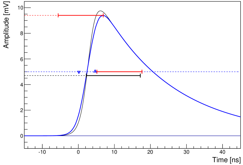
To illustrate the pulse extraction algorithm, an example pulse for a single discharge is shown in figure 1 as a thin black line.

The first twenty and last ten samples of each event are discarded because they suffer from additional noise. Before pulse extraction a sliding average filter of ten samples is applied, which is possible due to oversampling. This improves the signal-to-noise ratio and eliminates some occasional noise with a corresponding frequency. The resulting pulse shape is shown in blue. To identify the pulses, the samples are scanned for a leading edge defined as a threshold crossing between two consecutive samples. Studies have shown that good results are obtained with a threshold of 5 mV (dashed blue line). In addition, it is required that the amplitude four samples before and after the threshold crossing, is still below, respectively above the threshold, indicated by the two blue arrows. A local maximum is searched between five and 35 samples after the threshold crossing (bottom red line). Within a range of 30 samples before the determined maximum (top, red line), the last sample which does not fall below 50% of that maximum is sought. The position of this sample is called arrival time hereafter. If the distance between the maximum and the arrival time exceeds 14 samples (7 ns), the pulse is discarded as wrong identification. Starting from the arrival time, 30 samples of the raw signal are integrated, hereafter called extracted signal. The next search starts at the end of the integration window. To allow for a proper calculation of the dark count rate, the number of searched samples is computed as well.

An example of a spectrum obtained from a single channel in a single run is shown in figure 2.

2.1.3 Parameter extraction

In the obtained spectrum, the distance between two consecutive peaks represents a measurement for the charge released in a single breakdown, i.e. the gain. Higher order multiplicities reflect the process in which optical crosstalk spreads from a primary breakdown. The total number of detected signals is a measure of the dark count rate.

To get a more precise estimate of these properties, the spectrum of each individual pixel is fit to a corresponding distribution function. Empirically, it has been found that the best fit is obtained with a slightly modified Erlang distribution. This distribution describes the probability to measure a multiplicity of $N$ synchronous signals induced by a single primary breakdown. A more detailed discussion can be found in appendix A.

Spectrum function

While the modified Erlang distribution describes the distribution of the multiplicity $N$, for the proper description of a real measurement additional noise components have to be taken into account. Measuring a real sensor, the fluctuations on the released charge and electronics noise smear out the distribution. While electronics noise can be considered independent of the number of breakdowns, the fluctuation on the released charge scales with the multiplicity. Both types of noise are assumed to be Gaussian with width $\sigma_{el}$ for the constant noise and $\sigma_{pe}$ for the amplitude dependent noise.

The resulting distribution can be expressed as a sum of Gaussian functions for multiplicity $N$, each with the gain $g$ and a baseline shift $x_{0}$. The gain $g$ corresponds to charge extracted from a single avalanche. Therefore, in the following gain and extracted charge will be used interchangeably.

$$f(x)=A_{1}\cdot a_{1}\sum\limits_{n=1}^{n=\infty}P_{n}\,\frac{e^{-\frac{1}{2}\,\left[\frac{x-x_{n}}{\sigma_{n}}\right]^{2}}}{a_{n}}$$ (1)

with the offsets $x_{n}$, the width $\sigma_{n}$ and the normalization $a_{n}$

$$x_{n}=x_{0}+ng\,,\qquad\sigma_{n}=\sqrt{n\,\sigma_{pe}^{2}+\sigma_{el}^{2}}\qquad\mbox{and}\qquad a_{n}=\sigma_{n}\,\sqrt{2\pi}$$ (2)

and the modified Erlang distribution (see equation 25) as the distribution function $P_{n}$

$$P_{n}=\frac{(nq)^{n-1}}{\left[(n-1)!\right]^{\nu}}\qquad\mbox{with}\qquad q=p\cdot e^{-p}\,.$$ (3)

For easier determination of start values in a fit, the function is written such that $A_{1}$ denotes the amplitude of the single-p.e. peak. The normalized amplitude $A_{1}^{\prime}$ independent of the bin-width $w$ of the fitted histogram is then given as $A_{1}^{\prime}=A_{1}/w$.

Knowing the effective on-time $T_{eff}$ from the pulse-extraction, the dark count rate $R$ can be estimated as

$$R=\frac{A_{1}^{\prime}\cdot a_{1}\sum\limits_{n=1}^{n=\infty}P_{n}}{T_{eff}}\,.$$ (4)

The crosstalk probability $p_{xt}$ is

$$p_{xt}=\frac{\sum\limits_{n=2}^{n=\infty}P_{n}}{\sum\limits_{n=1}^{n=\infty}P_{n}}\,.$$ (5)

Fit procedure

Figure 2: Example for the spectrum of charges extracted from a single run and one pixel fitted with a modified Erlang distribution (red line). The plateaus close to the x-axis are artifacts introduced by the used plotting tool.

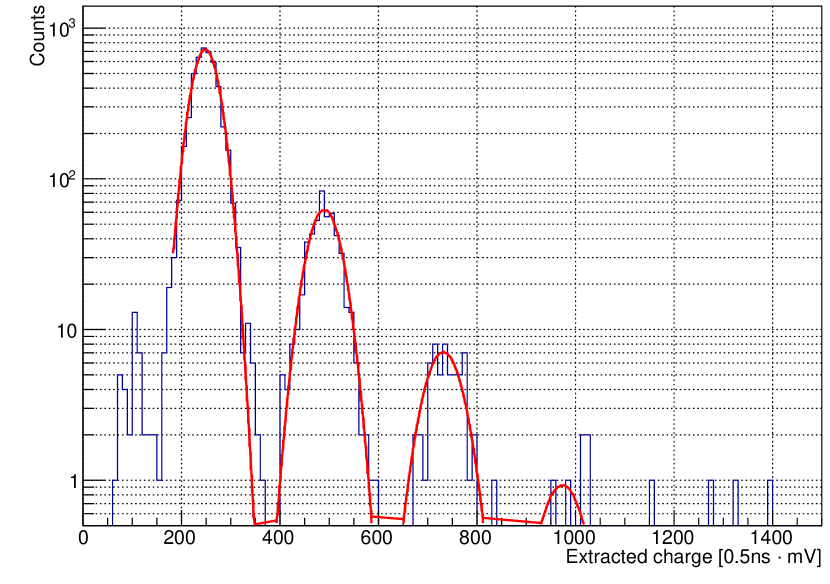
To obtain reasonable fit results, meaningful start values need to be obtained for all channels. This is achieved by fitting a high statistics spectrum, combined from all channels. An example of a randomly selected single pixel spectrum with the corresponding fit is shown in figure 2.

2.1.4 Offset calibration

Although during measurement, the feedback system keeps the gain stable, it does not yet calibrate its absolute value. Such a systematic offset can, for example, originate from inaccurate knowledge of the serial resistances or other systematic errors as mentioned in table 1. Since the sum of all systematic errors can easily exceed the precision of the voltage setting, an additional absolute calibration is required. Strictly speaking, a correction not only for offset but also for slope is necessary, for both, temperature and current coefficient. The influence of an imprecise slope can be neglected for the operational range of only a few volts. A simple voltage offset per channel is already enough to push the systematic error below the precision of the voltage setting.

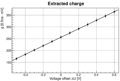
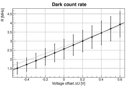
To calculate these offsets, the gain is determined from data taken at different voltages. An example of such a measurement is shown in figure 3 (top left). The data represents the average obtained from all channels and measurements taken at the same voltage, the error bars the standard deviation. From a linear fit to this average, the nominal gain at $\Delta U=0$ V is obtained. To obtain a reference for each individual bias voltage channel, the readout channels belonging to one bias channel are averaged and fit linearly as well. From these fit and the nominal gain, a voltage offset for each channel is calculated and applied.

2.2 Results

With the determined offsets applied, measurements were taken to determine also the dependency of the variables on voltage. Dark count spectra obtained from runs taken at varying ambient temperatures allow for the determination of the dependency on the sensor temperature.

2.2.1 Voltage dependency

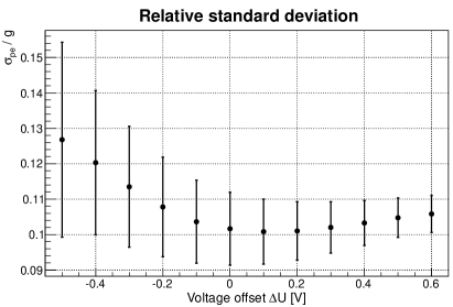
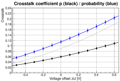
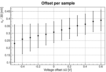
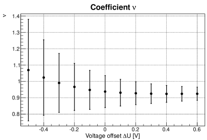
To derive the voltage dependency, in total 10 measurements where taken at 14 voltages, each between 14/03/2014 and 17/03/2014 at average sensor temperatures between 8.4 °C and 10.7 °C. From the parameters obtained by the fit, their average for each voltage is calculated. The results are shown in figure 3. The error bars represent the standard deviation of the parameters obtained from all measurements and channels. The larger ones are dominated by the change of the parameters with sensor temperature, see section 2.2.2. The increasing standard deviation and fluctuations towards lower voltages are due to a significantly decreasing fit quality introduced by a worsening in separation of the individual peaks in the spectrum.

To describe the voltage dependency of all variables, the following function has been fit to the dark count rate, the gain, the noise relative to the gain, the crosstalk coefficient and the crosstalk probability as shown in figure 3. The baseline and the coefficient $\nu$ of the modified Erlang distribution can be considered constant within the obtained statistical errors.

Par($\Delta U$)	$c_{0}$	$c_{1}$	$c_{2}$
Dark count rate $R$	(1.8 $\pm$ 4.7) MHz	1.4 $\pm$ 2.2	1.1 $\pm$ 2.0
Extracted charge $g$	181 $\pm$ 6	1.42 $\pm$ 0.04	1 (fixed)
Crosstalk coefficient $p$	0.03 $\pm$ 0.03	1.5 $\pm$ 0.6	1.8 $\pm$ 0.7
Crosstalk probability $p_{xt}$	0.07 $\pm$ 0.05	1.4 $\pm$ 0.5	1.62 $\pm$ 0.6

Table 2: Coefficients obtained from the fits of the function given in equation 6 to the measurements as shown in figure 3.

Figure 3: Average of the fit parameters of all channels obtained from several measurements. Each measurement contains data taken at 14 different voltages. An offset of 0 V corresponds to the operation voltage of the sensors. Error bars show the standard deviation of the obtained parameters. Data was taken at sensor temperatues between 8.4 °C and 10.7 °C. The gray dashed lines are measurements taken by [8] for a similar sensor type. Their dark count rate measured for a 1 mm² sensor was scaled linearly to 9 mm² for an easier comparison. The crosstalk values refer to the probability $p$ as obtained from the fit (black) and the crosstalk probability (blue).

$$Par(\Delta U)=c_{0}\cdot\left[\frac{\Delta U}{\mbox{V}}+c_{1}\right]^{c_{2}}$$ (6)

The resulting coefficients are summarized in table 2.

For comparison, measurements obtained in [8] for the dark count rate and the crosstalk probability are shown as gray dashed line. As their measurements have been carried out for a slightly different type of sensor (50 $\mu$m cell size, 400 cells) a perfect match is not expected. To achieve comparability, their dark count rates have been scaled up linearly to an area of 9 mm². It is known, that dark count rates for the same sensor type can change already from production to production due to the purity of the silicon. Taking also into account that both measurements have most probably been taken at different temperatures, their slopes and even their absolute values fit surprisingly well.

Overvoltage

From the extrapolated voltage offset at which dark count rate, gain and crosstalk vanish, the overvoltage can be derived. While dark count rate and crosstalk depend on absolute temperature as well, the effect on the gain is fully compensated by the feedback system. This is illustrated by the small error bars demonstrating the small variation between the measurements. Therefore, the gain is the best measurement for the overvoltage consistent with the results obtained from the other parameters. Using the definition of overvoltage from section 1.3, the fit shown in figure 3 (top left) and the corresponding fit as presented in table 2 suggest that the operation voltage of the sensors correspond to an overvoltage of 1.4 V which is consistent with the datasheet of the devices.

2.2.2 Temperature dependency

The temperature dependency of the coefficients is derived from 295 runs taken between 11/01/2014 and 21/03/2014 at average sensor temperatures ranging from 4 °C to 19 °C. From the fit results to all measurements, average and standard deviation of all channels are calculated.

Figure 4: The average of the extracted charge obtained from all channels versus the air temperature in the container hosting the bias power supply. A clear linear dependency can be seen corresponding to less than 1‰/°C in absolute voltage. The effect most probably originates from the calibration resistor or the op-amp driving the power supply circuit.

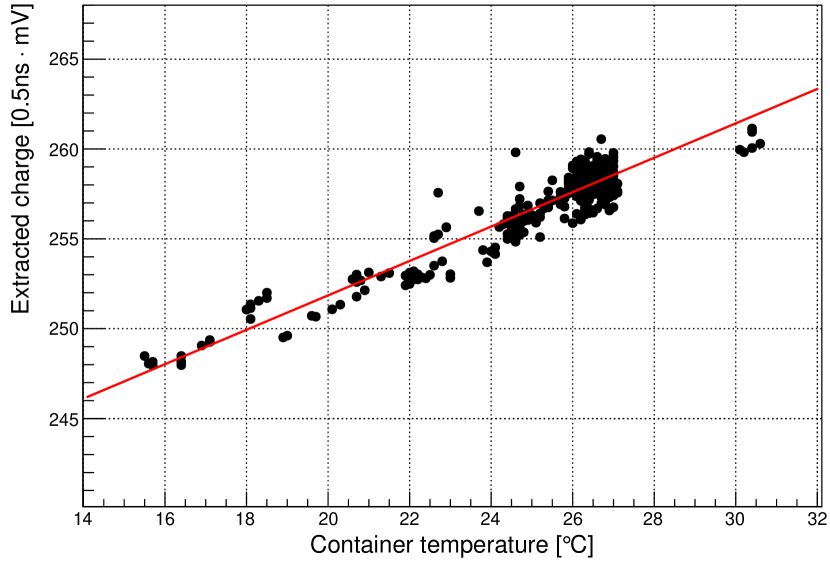
Surprisingly, a dependence of the gain on the air temperature of the container in which the bias power supply is hosted has been found, as shown in figure 4. Investigating the data further, it turns out that only a fraction of the bias channels show this effect while channels hosted on two boards out of eleven are not affected. This makes an individual calibration of every channel necessary. Although this is doable, the missing control over the temperature renders a calibration very difficult. The most reasonable explanation is that two different charges of either the calibration resistor or the op-amp have been used in assembly and one of them has a higher temperature gradient. The observed dependency is about 4% over 10 °C corresponding to less than 1‰ in absolute voltage which is on the order of the typical temperature gradient of some commercial resistors. Fortunately, the container is air conditioned and heat waste from the electronics generates a stable temperature most of the time. In special conditions like strong winds, clouds or fog on exceptionally cold days, the temperature can still drop which creates the observed effect. Although this affects the gain only on a few days a year, it is planned to either replace the boards or stabilized the temperature. To get an unbiased result, runs taken at measured container temperatures below 25.5 °C and above 27 °C have been rejected so that for the analysis the whole range is restricted to roughly 1 °C. This range contains the majority of the data points, as it can be seen in figure 4.

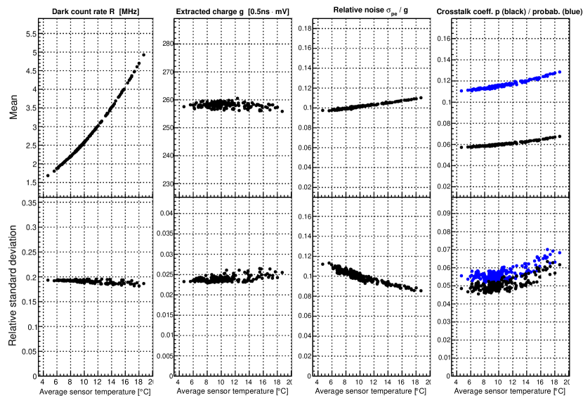
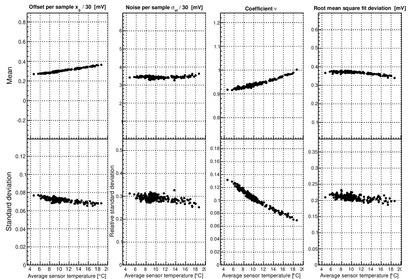
An overview of the results of the measurement of the temperature dependecy is shown in figure 5. The crosstalk shows a small residual temperature dependency. This can be interpreted as a dependency on the absolute voltage. In this study, both effects can not be disentangled. The dark count rate shows the dependency on temperature expected from the data-sheet. The distribution coefficient $\nu$ shows a dependency, although this affects only multiplicities larger than $N\sim 7$. It might as well be related to small changes in the efficiency of the charge extraction algorithm for $N=1$.

Fitting a polynomial of second order to the dark count rate and the crosstalk coefficient yields the results given in table 3.

Figure 5: Result from the fit to the recorded dark count spectra at different sensor temperatures. Shown is the average and standard deviation of the values obtained from all channels for one run. For all values except the offset $x_{0}$ the standard deviation is expressed relative to the mean.

	$c_{0}$	$c_{1}$	$c_{2}$
Dark count rate/MHz	1.263 $\pm$ 0.006	0.0587 $\pm$ 0.0012	0.00730 $\pm$0.00005
Crosstalk coefficient	0.0558 $\pm$ 0.0003	(1.7 $\pm$ 0.5)$\cdot 10^{-4}$	(2.362 $\pm$0.022)$\cdot 10^{-5}$

Table 3: Coeffients of a fit of a second oder polynomial to the temperature dependence of dark count rate $R$ and crosstalk coefficient $p$ as shown in figure 5.

The distribution of most fit values in the camera scales nicely with the value itself so that the relative standard deviation is mainly temperature independent. The distribution of the relative noise $\sigma_{pe}$ and the coeffiecient $\nu$ becomes smaller with increasing temperature which can be attributed to the increased number of available freedoms to fit, more precisely the higher multiplicities available in the distributions. This is an effect of the increased crosstalk probability. It is also supported by the slightly increasing fit quality expressed by the root mean deviation between the distribution and the fit function.

2.2.3 Gain stability

Figure 6: Run-wise mean (top) and standard deviation (bottom) of the extracted charge $g$ of all channels versus average sensor compartment temperature (left) and as distributions (right). No significant dependency on temperature is visible. The width of the distribution of means is $\sim$3‰. Two gray dashed lines denote the mean $\pm$1%. The average standard deviation is around 2.4%.

Figure 7: Randomly selected example distributions. The left plot shows the distribution of the gain of all individual channels normalized to the average gain. The standard deviation of this distribution is $\sim$2.4%. The right distribution shows the standard deviation of the gain per bias channel relative to its average. For an operation voltage which corresponds to an overvoltage of 1.4 V, its average of 2.1% corresponds to a voltage of $\sim$29 mV.

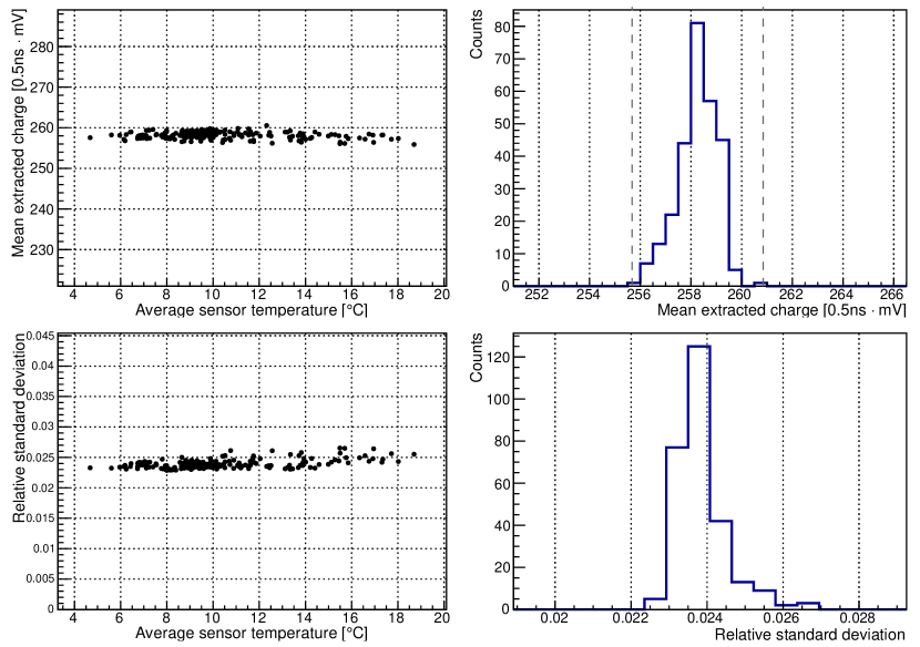
One of the most important results for this project and for future detectors is the stability obtained for the gain using G-APDs under real environmental conditions. In figure 6, the mean and standard deviation of the average extracted charge over all channels is shown versus average sensor temperature together with their corresponding distributions. The standard deviation of the distribution of the measured average gain values is $\sim$3‰. The average of the standard deviation of the distribution of the gain values in the camera 2.4%. Although this standard deviation is in the order of the expectation from the precision of the hardware and feedback values, it still means that the maximum deviating channels reach out to almost $\pm$10% due to the high number of channels. The average standard deviation within single patches is on the order of 2.1% and independent of the temperature. For an assumed overvoltage of 1.4 V this corresponds to 29 mV. This value fits reasonably well with the precision with which the operation voltages was specified by the manufacturer used to sort the sensors into patches and the precision of the individual serial resistors. An example distribution for the gain of all channels relative to the average gain and an example distribution for the patch standard deviation is shown in figure 7. For single sensors, this result means that they stay within the achievable limit defined by the hardware voltage setting, otherwise the standard deviation would be increased. Apart from the large number of sensors, the full width of the distribution can be explained with the standard deviation of values within patches of up to 4% plus the 2.2% shift introduced from a single voltage step.

2.2.4 Sum spectra

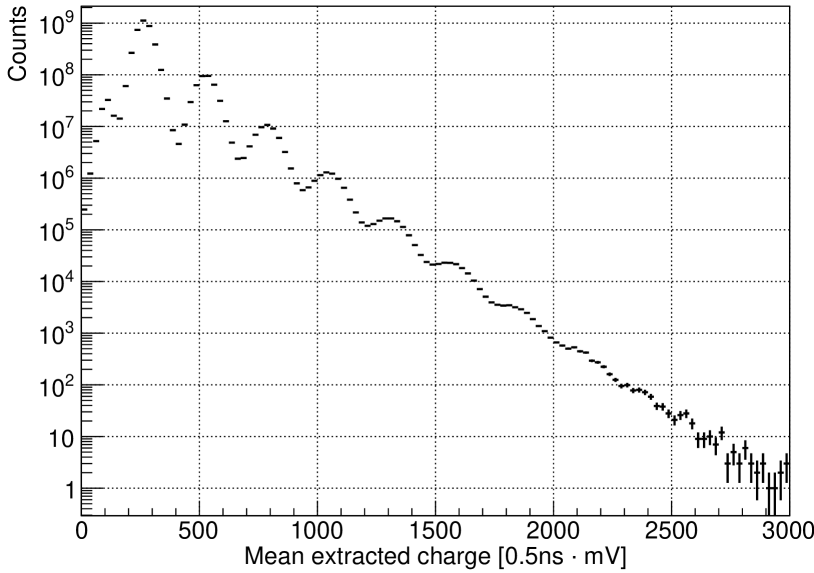
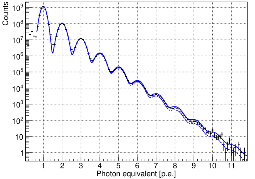
Due to the very small variation of the gain, all measured spectra can be combined into a single spectrum, as shown in figure 8 (top). The peaks from individual breakdowns can easily be distinguished up to a multiplicity of $N\sim 7$. This result improves further, when all individual spectra are offset ($x_{0}$) subtracted and normalized with the determined gain $g$. This result is shown in figure 8 (bottom). Here, multiplicities up to at least $N=10$ can be distinguished. The high level of similarity between the scaled and unscaled distributions proves not only the stability of the system and the successful operation of the feedback system but also the precision of the applied charge extraction. The overlaid fit of a modified Erlang distribution (solid) and a standard Erlang distribution (dashed) proves the applicability of these distributions up to very high multiplicities. A difference between both is only visible for multiplicities $N>5$.

The fit results for the modified Erlang distribution with $g=1$ and $x_{0}=0$ are summarized in table 4. The relative errors of all parameters are in the order of $10^{-4}$ or smaller. The corresponding crosstalk probability $p_{xt}$ according to equation 5 is 11.7%.

Parameter	$A_{1}$	$\sigma_{pe}$	$\sigma_{el}$	$p$	$\nu$
Value	$1.2282\cdot 10^{9}$	0.10469	0.060770	0.070314	0.93715

Table 4: Resulting coefficients from fitting a modified Erlang distribution to the sum spectrum shown in 8. All significant digits according to the obtained statistical errors are provided.

If in a camera with 1440 sensors, a rate of avalanches per channel between 50 MHz and 2 GHz induced by night-sky background photons is expected, this gives a total rate between 72 GHz and 2.9 THz. Taking the fit result for the spectrum in figure 8, this yields roughly one event per second with a multiplicity of $N$ = 15 in low light conditions and one with $N$ = 18 for bright light conditions excluding possible pile-up from the night sky itself. Including fluctuations, it can be assumed that with a trigger threshold of at least 20 p.e. ($N$ = 20) not more than one trigger per second is induced by optical crosstalk events.

Figure 8: Top: The sum of all dark count spectra. Different peaks can easily be distinguished up to $N\sim 7$. Bottom: Sum of the same spectra, but each one normalized individually with the extracted offset and gain. Overlayed is a fit of a modified Erlang distribution (solid line, top) and an Erlang distribution (dashed line, bottom). More detail given in the text.

2.2.5 Pulse shape

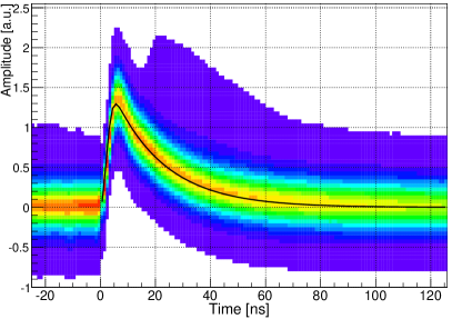
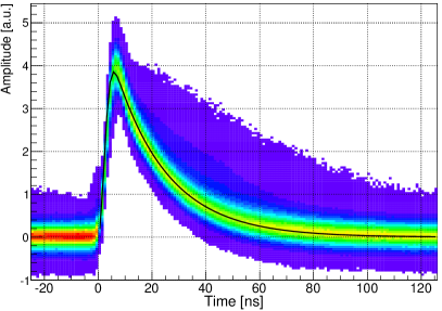
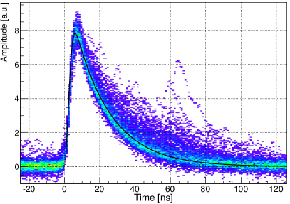
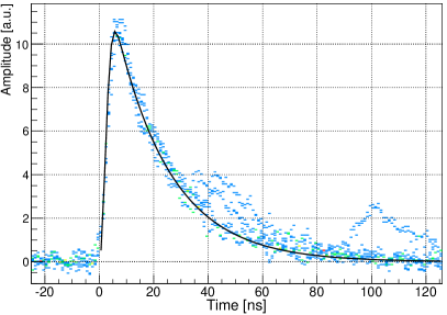
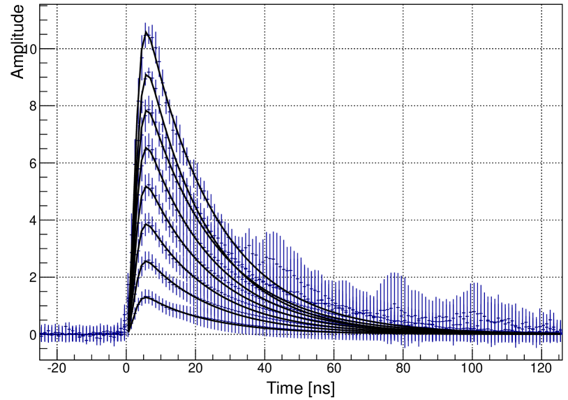
The average gain of each channel can be used to scale the extracted pulses and overlay them shifted by their arrival time. From this, two dimensional histograms were filled and profiles calculated, separated for different multiplicities, for example, for multiplicity $N$ = 1 for extracted signals between $0.5g$ and $1.5g$. The result for a randomly selected run at nominal operation voltage can be seen in figure 9. A very good match of individual pulses is evident. Also visible is the influence from afterpulses. Since their amplitude is attenuated by the amount of remaining charge in the cell and at the same time their probability is exponentially decreasing, they show an activity maximum a few nanoseconds after the primary pulse. If the range in which a pulse is integrated is chosen carefully, the bias from afterpulses can be suppressed completely.

To all profiles, the following function has been fit between 1 ns and 25 ns:

$$A(t/\mbox{ns},N)=c\,N\cdot(1-\frac{1}{1+e^{\frac{t-t_{0}}{\tau}}})\cdot e^{-\frac{t-t_{0}}{\lambda}}$$ (7)

The shift of function with respect to the extracted arrival time is a priori unknown, therefore a free parameter for the time shift $t_{0}$ is introduced. If the charge scales with the multiplicity $N$ as expected, the normalization $c$ should be independent of the multiplicity. The rise and fall times are described by $\tau$ and $\lambda$ respectively. Its maximum is reached at $t=t_{0}+\tau\log(\lambda/\tau-1)$. The fit range was chosen to suppress the effect of afterpulses and optical crosstalk events induced from afterpulses. The results of the fits for different multiplicities are summarized in the table 5.

N	$c$	$t_{0}$/ns	$\tau$/ns	$\lambda$/ns
1	1.57 $\pm$ 0.20	2.7  $\pm$ 0.5	0.9  $\pm$ 0.3	19 $\pm$ 5
2	1.57 $\pm$ 0.13	2.8  $\pm$ 0.3	1.05 $\pm$ 0.19	19 $\pm$ 3
3	1.59 $\pm$ 0.10	2.8  $\pm$ 0.3	1.07 $\pm$ 0.16	19.3 $\pm$ 2.6
4	1.60 $\pm$ 0.08	2.8  $\pm$ 0.3	1.07 $\pm$ 0.16	19.4 $\pm$ 2.2
5	1.62 $\pm$ 0.07	2.86 $\pm$ 0.23	1.09 $\pm$ 0.14	19.4 $\pm$ 1.9
6	1.62 $\pm$ 0.07	2.91 $\pm$ 0.23	1.14 $\pm$ 0.14	19.9 $\pm$ 1.9
7	1.63 $\pm$ 0.03	3.00 $\pm$ 0.14	1.04 $\pm$ 0.08	18.2 $\pm$ 0.7
8	1.62 $\pm$ 0.04	2.74 $\pm$ 0.20	1.07 $\pm$ 0.10	20 $\pm$ 1.0

Table 5: Resulting coefficients of fitting the pulse shape described by equation 7 to the pulse profiles as shown in figure 9.

Applying the signal extraction used for the dark count spectrum to the fit functions, or integrating the pulse from half-height-maximum for 15 ns, leads to a charge consistent with the expected linear behavior within errors. This match is illustrated by the good match of all eight pulses re-normalized with $c_{0}$ = 1, $c_{1}$ = 0 and $N$ = 1. This is shown in the inlay in figure 9 (bottom). This is consistent with the expectations taking the band width of the readout chain into account.

Figure 9: Two dimensional histograms (top) of the sampled waveform. The color scale starts at 0.5% of the maximum bin. The shown multiplicities are 1, 3, 6 and 8 (top left to bottom right). For all multiplicities between one and eight, a profile histogram has been filled (bottom). Fits to the profile histogram are shown as black lines. The inlay shows all eight fits re-normalized with $c_{0}$ = 1, $c_{1}$ = 0 and $N$ = 1. A good agreement is visible.

3 Light pulser measurements

The evaluation of dark count spectra taken with closed lids cannot measure the dependence of the gain from the current, i.e. the ambient light condition. Instead, the measured amplitude of an external light pulser is used. The light pulser is installed in the center of the reflector dish. Its light yield is temperature stabilized.

For each measurement, the light pulser is flashed one thousand times with a rate of 25 Hz. The readout is self-triggered by the camera’s trigger system. To avoid triggers on showers, the time window for each trigger is only 12 ns and a trigger signal from at least 25 out of 40 trigger boards is required.

Light pulser runs are currently taken roughly every 20 minutes during standard data taking. The data from the 650 analyzed runs presented here were taken between 31/12/2013 and 21/03/2014. During all measurements the feedback system was in operation.

3.1 Method

Signal extraction

After the digital values have been converted to physical units, the signal is extracted by a peak-search and an integration of 5 ns before and 80 ns after the half-height leading edge. To determine the maximum and the position of the half-height leading edge, a 3 order spline interpolation is applied. For each channel, the average amplitude of all events is calculated.

The emitted pulses have a typical length of 50 ns with an average amplitude of $\sim$30 p.e. per pixel. Although the event-to-event fluctuation of the amplitude is comparably large, it is stable on average.

Light pulser properties

Laboratory measurements have shown that a small temperature dependency of the light yield still remains. As the correlation of the measured amplitude on the ambient temperature is stronger than on the sensor temperature, it can be assumed that this is an effect of the light pulser exposed to ambient temperature rather than of the gain of the sensors. This is also justified because the amplitude increases with increasing temperature. In the case that this would be an effect of the gain of the sensors, the measured temperature had to be higher than the real temperature of the sensor so that the feedback system would apply a too high voltage. As the main heat source in the sensor compartment are the sensors themselves, there is no reason to assume that with increasing current a temperature measured close to the sensors is overestimated. Therefore, the residual temperature dependency has been fitted with a line with a slope corresponding to $\sim$5%/$100\,\mu$A and the data has been corrected accordingly.

The light emitted by the pulser is spatially inhomogeneous on the camera surface to within a few percent. The light distribution is approximated with an average amplitude distribution from all data taken under moonless conditions with $I<7\,\mu$A for which the smallest influence is expected. For this study, it has then been subtracted patch-wise from all runs.

Another bias on the measurement is the tidiness of the light-emitting diode. Small jumps of the measured amplitude are observed between consecutive nights, especially after rain, fog or snow.

3.2 Results

Figure 10: Run-wise mean (top) and standard deviation (bottom) of the light pulser amplitude from 1428 channels versus median per-sensor current (left) and as distribution (right). Blue denotes the standard deviation of the amplitude distribution, corrected for the inhomogeneous illumination of the camera surface.

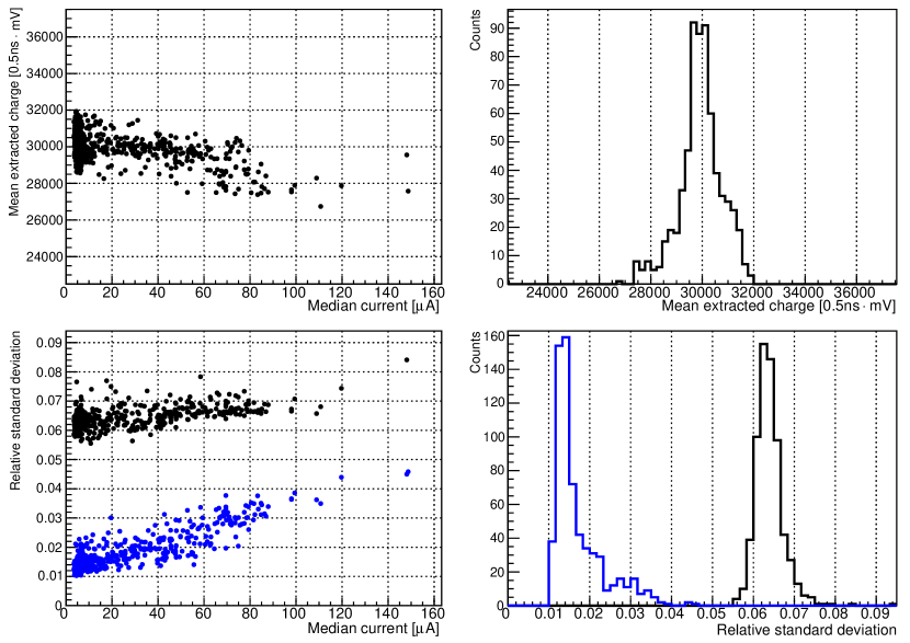
The results of the measurements are shown in figure 10. Each entry represents the mean (top) or sigma (bottom) of a Gaussian fitted to the distribution of the average amplitude of all 1428 channels per run. Black denotes the uncorrected distribution, blue denotes the distribution corrected for the average light distribution. In the following, the indicated current is the average of the currents determined for the individual sensors to avoid the ambiguity from a different number of pixels served by different voltage channels. A current of 100 $\mu$A therefore gives a current in the bias channel of 400 $\mu$A or 500 $\mu$A depending on whether four or five sensors are served by this channel. While the mean (top left) shows a decrease between new moon ($\sim$5 $\mu$A) and bright moon light conditions ($\sim$100 $\mu$A), the sigma (bottom, left) shows an increase.

The decrease of the average amplitude between new moon and bright moon light conditions is on the order of 5%. This trend is independent of the applied temperature correction. The standard deviation of the distribution is smaller than 3%.

Both trends are due to inhomogeneities in the amplitude distribution appearing in the camera with increasing current. Looking into the data in more detail, it turns out that while the majority of the pixels still shows the nominal expected value, large scale patterns which show lower amplitude exist. Runs taken at different pointing directions and different moon positions show different patterns.

The reasonable explanation found for the decrease with increasing current, could be that the temperature of the sensor compartment is dominated by the waste heat of the sensors themselves. At a voltage of $\sim$70 V and a current of 100 $\mu$A per sensor, the sensors dissipate a total power of $\sim$10 W. Generally, waste heat is dissipated through the solid cones, the photo sensor’s carrier and the air. Especially at high currents, a fraction of the waste heat is lost through the solid cones. Therefore the temperature at the temperature sensors slightly smaller than of the photo sensors themselves which in turn facilitates a too low applied voltage. While an 8% decrease can be explained with the temperature difference of only 2 °C, a mismatch in resistor value or current measurement of 8% is unlikely within the small range of operation compared to the full available range. Former studies did not show this trend hidden by the larger spread of the data due to the lower resolution of the applied analysis.

Another possible explanation could be the decrease of detection efficiency at bright light conditions because on average a finite number of G-APD cells recently suffered a breakdown and are recharged. Taking the spectrum of the diffuse night-sky background and the spectral response of the instrument into account, the rate of induced avalanches per sensor under new moon conditions does not exceed 50 MHz, corresponding to $\sim$5 $\mu$A. The brightest conditions, corresponding to a $\sim$98% illumination of the moon disk, produced a current of not more than 200 $\mu$A. Which is the maximum at which regular observations have been carried out so far. For a dark count rate of 5 MHz and a dark current of 0.5 $\mu$A a corresponding rate of $\sim$2 GHz for breakdowns per sensor can be deduced. Taking the determined pulse shape as reference with a half-value time of 20 ns, this yields on average 1% of cells which show no or a significantly reduced response. Taking 100 ns until the cell is fully recharged, on average another 4% of all cells will show an attenuated signal. That means that even during the brightest observations ever recorded, the detector efficiency was not reduced by more than 5%. Taking the average of the released charge, the decrease will not be more than 2%. Consequently, at 100 $\mu$A the effect is negligible and cannot explain the measured 5% decrease.

The uncorrected standard deviation in the camera is between 6.5% and 7%. Correcting for the average light distribution during new moon nights, it increases from $\sim$1% to a maximum of 4% during bright moon light conditions. This increase is expected for several reasons: The brighter the ambient light gets the more inhomogeneous the background light yield in the camera becomes due to direct moon light, reflections and shadowing. While the purpose of the feedback is to correct this effect, it can only be corrected on average per bias voltage channel, but not for the individual sensors connected to each channel. Consequently, the distribution is expected to get broader, the more inhomogeneous the background light becomes. In addition, the noise in the readout increases with the square-root of the background light flux which directly affects the variation of the reconstructed amplitude especially at bright light conditions. This is supported by the fact that at low currents the event-to-event variation correlates with the average amplitude. This effect vanishes towards higher currents. A possible underestimation of the sensor temperature has been discussed previously.

4 Ratescans

With the measurement of the dark count spectrum and the light pulser amplitude, the stability of the system in terms of temperature and ambient light conditions has been demonstrated. In both cases, only the response of a fraction of the whole system is taken into account and the light pulser measurement shows influence from the properties of the light pulser itself. Instead, ratescans offer the possibility to directly measure the detector response on ambient light and air showers. Ratescans determine the detector’s trigger rate as a function of the trigger threshold. At low thresholds, this rate is completely dominated by triggers induced randomly from night-sky background photons. At high thresholds, triggers by air showers or their secondary particles dominate. At low thresholds, the total trigger rate is the sum of the triggers of all trigger channels because triggers of individual channels are independent. At high thresholds, the total trigger rate is lower than the sum of the individual trigger channels because in most cases several patches trigger in coincidence.

To understand this in more detail, the trigger hardware is outlined hereafter. A more detailed description is available in [2].

4.1 Method

Trigger system

First, an analog sum of the nine signals of the channels corresponding to one four- and one five-pixel bias voltage channel is performed. Clipping is used to shorten the length of the output signal. Next in line is a comparator whose threshold is set by a 12 bit digital-to-analog converter. Roughly 15 counts correspond to the amplitude of a single photon equivalent. As the conversion is not precise but depends on many factors, as for example the gain of the sensors, in the following only counts are used, although this number allows for an estimate of the amplitude in units of photon equivalents. The comparator signal from four patches is summed serving as input for a 1-out-of-4 discriminator logic. Requiring a minimum length of its input signal, this logic suppresses electronics noise. The final trigger decision is a simple OR of the incoming discriminator signals, more precisely the result of a N-out-of-40 logic realized in a Field Programmable Gate Array (FPGA) with N = 1.

To monitor the rate of all trigger channels, a counter for all comparator and discriminator outputs as well as a counter for the final trigger decision is implemented in the controlling FPGAs. Their readout time is set to once every second during ratescans and once every five seconds during data taking.

Measurement

Under normal data taking conditions, one or two ratescans are performed every night. They typically last about five to ten minutes. For a pointing direction, a sky region without bright stars is chosen with a zenith distance not more than 25°. This avoids bias from bright stars in the field-of-view and increased attenuation towards the horizon. Ratescans taken under verifiable non-ideal weather conditions have been discarded. Each measured point contains at least 400 triggers so that a statistical error of at least 5% is achieved for the total trigger rate. Ratescans are started at a threshold of 100 and stopped when the time needed to collect enough data to achieve the 5% statistical error exceeds 2.5 minutes.

4.2 Results

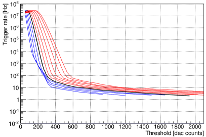
To better understand the effect of different gains on the rates, ratescans with different bias voltage settings were taken. The measurements in figure 11 (left) were recorded during a single dark night at voltage offsets from the operation voltage between -0.4 V and +0.6 V in steps of 0.1 V corresponding to an overvoltage between 1.0 V and 2.0 V. These ratescans have been taken at zenith distances smaller than 20°. Each ratescan typically shows three different regions. At very low thresholds, a saturation of the counter is visible, followed by a steep slope dominated by triggers induced from ambient photons. After a transition, a long and flat tail is visible representing air showers induced from cosmic rays.

Figure 11: Ratescans taken in one night (01/02/2014) during good atmospheric conditions with different applied voltages. The applied voltage has an offset from the nominal voltage between -0.4 V and 0.6 V in steps of 0.1 V. Curves with voltages lower than the nominal voltage are shown in blue, curves with higher voltages in red. The curve at nominal voltage is shown in black. The left plot shows the curves as recorded, the right after applying a scale factor. The scale factor was determined manually for best fit and then fitted (bottom). A good match of the shower tail is observed. More visible details are explained in the text.

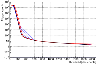
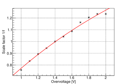
As the change in voltage implies a change in gain and respectively in threshold, it should be possible to rescale the threshold value according to the applied voltage to match one another. To obtain this match, an additional artificial scale factor $f$ is necessary, to correct for changes in photo detection efficiency and crosstalk probability. Such an artificial factor has been applied manually until all curves matched the reference curve at nominal voltage. The derived scale factors are shown in figure 11 (bottom). They have been fitted with $1/f=(2.15\pm 0.13)[1-e^{(0.45\pm 0.04)\cdot U}]$ and the corresponding resulting factors applied. The scaled curves are shown in figure 11 (right). The cavity visible around the kink for low voltages originates from noise of the digital electronics and is related to the readout of the counters and the switching of the comparators and discriminators.

The good match of the scaled curves proves the stability of the system. The unscaled curves show that a change in gain would generate a rescaling of the threshold value appearing as a shift of the shower tail.

The small gap in the falling edges is due to the change of pointing direction which induced a small change in ambient light level. Generally, a small shift towards higher thresholds and a steepening of the slope is visible with increasing voltage. This is most probably a direct effect of the increase of photo detection efficiency and crosstalk probability.

The curves with the highest overvoltages show a saturation at around 2 Hz for high thresholds. It is assumed that this originates from two faulty channels. In these channels, the serial resistor is too low and therefore the voltage at the G-APDs far higher than nominal. Consequently, they show a significant increase in crosstalk probability and a finite probability that a single breakdown eventually induces a discharge of all cells in the sensor. Although the trigger input for these two channels is disabled, such a high signal leads to electronic crosstalk in neighboring channels. Under normal data taking conditions, this can be neglected because the induced random triggers are well below normal data taking rates. With the additional increase of voltage, it becomes significant and is therefore visible in the plots as a saturation at high thresholds.

Figure 12: Ratescans taken close to zenith at good atmospheric conditions (left) but at ambient light levels ranging from new moon to almost full moon. The blue line is a selected reference ratescan. A good agreement of the shower tail independent of the ambient light level can be seen. The right plot shows ratescans taken under known poor atmospheric conditions as clouds (blue) and Calima (red). For comparison, the reference ratescan is shown as well (black). The effect of non ideal conditions is apparent. For easier comparison, the bottom plot shows two ratescans taken under comparable conditions at two different nights: Jan. 1 2014 (blue) and Feb. 1 2014 (black). The gray curves show the 40 individual board rates. An almost perfect match is visible. The small difference in the falling edge is due to a slightly different background light level.

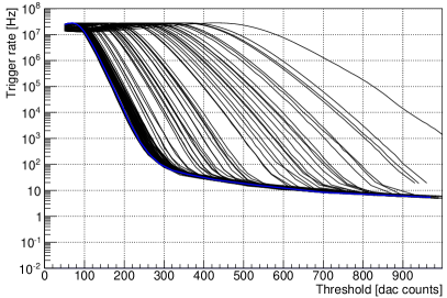
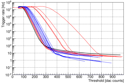
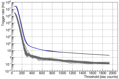
To prove a stable shower tail independent of light conditions, ratescans have been recorded between 08/10/2013 and 21/07/2014 at different light levels. They are shown in figure 12 (left). The light conditions range from new moon to more than 90% moon disk. A very good agreement of the shower tail of all curves is visible. At the same time, the changing light levels produce a shift of the falling edge. They all agree well within their statistical error which is in the order of 15% for low count rates. As an example for the good match, two ratescans taken in two different nights one month apart are shown (bottom) including the 40 discriminator rates. For comparison, the right plot shows selected rate scans taken under poor weather conditions such as thin cloud layers (blue) or Calima (red), a dust layer of Saharan sand in the atmosphere, c.f. [14], and the reference ratescan (black) from the left plot. Clearly visible is the strong influence of increased absorption in the atmosphere on the shower tail. Consequently, comparing the measured shower rate at a given threshold within the shower tail with the expected shower rate can reveal valuable information about data quality and for data analysis, c.f. [15].

5 Threshold parametrization

To better understand the relation between the kink of the ratescans and the ambient light level, all ratescans were parametrized and fitted. The parameters obtained from the fits were used to determine a relation between the measured current and the threshold.

Method

A function of the rate $R$ versus threshold $t$ has been fitted to all ratescans:

$$R(t)/\mbox{Hz}=R_{0}(t)+R_{1}(t)$$ (8)

with

$$R_{0}(t)=e^{m\cdot(t-t_{0})}\qquad\mbox{and}\qquad R_{1}(t)=1.8\cdot 10^{9}\ t^{-3}+3.5$$ (9)

Figure 13: Coefficients from the fit to several ratescans at different ambient light level. Details and the result of the fits (red) can be found in the text.

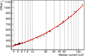
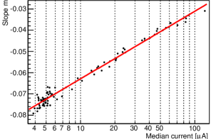
The function $R_{0}$ denotes the rate of triggers from random photons and $R_{1}$ the rate of triggers from coincident photons, or ambient light and showers, resp. The function $R_{1}$ was fit independently for $t$ ¿ 350 on the reference ratescan shown in figure 12. The starting point of all fits is chosen such that only the mainly exponential part of the falling edge just before the kink is considered.

Result

The resulting coefficients $m$ and $t_{0}$ are shown in figure 13 as a function of the median current of all bias voltage channels. Fits to the data yield

$$m=(-0.0947\pm 0.0005)+(0.0318\pm 0.0005)\cdot\mbox{ln}\left(\frac{I}{\mu\mbox{A}}\right)$$ (10)

and

$$t_{0}=(192.0\pm 1.6)\left(\frac{I}{\mu\mbox{A}}\right)^{0.3500\pm 0.0024}\,.$$ (11)

Figure 14: From the fits to all ratescans, the point at which the trigger rate from background photons falls below $1/e$ of the rate from the shower tail is determined. The result for the corresponding thresholds is shown versus the median current in the camera. Details on the function which was fit to the data (red) can be found in the text.

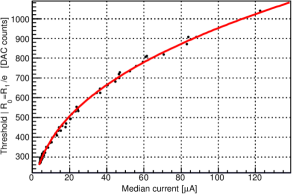
For each fit, the threshold at which the condition $R_{1}=R_{0}/e$ is fulfilled is determined. The result is shown in figure 14. A fit to the data provides the following relation for the threshold $t$:

$$t=(156.3\pm 1.2)\left(\frac{I}{\mu\mbox{A}}\right)^{0.3925\pm 0.0022}$$ (12)

This result does not describe the attenuation of the shower tail by changing atmospheric conditions or with increasing zenith distance. Both effects are neglected in view of the very steep edge induced by triggers from background photons.

Application

For more than a year, the obtained relation between threshold and current is used during data taking to set the trigger threshold of all comparators. Just before a run is started, the median current is determined and the threshold level set accordingly. To avoid a bias on the analysis due to changing thresholds, the threshold level is kept constant during runs. Only single channels with high rates due to direct star light are continuously regulated. Due to the fast changing ambient light level during twilight, runs with only one minute instead of the usual five minutes are taken. Under normal circumstances, all other fluctuations during the night are slow enough to not result in too high rates within this five minute interval. In rare cases of sudden rise of brightness, like overclouding or direct light from cars passing by on the nearby road, it can happen that the data acquisition saturates, but in these cases data are not suited for further analysis anyway.

The application of the derived threshold has lead to very stable rates and observation conditions. Currently, exceptionally high rates from single patches, like bright stars, are still suppressed with an algorithm based on the measured patch rates, but efforts are ongoing to base that on their individual currents as well. The lowest threshold achieved during clear new moon nights is on the order of 300 counts which corresponds to roughly 20 p.e. per trigger patch or $\sim$2.2 p.e. per pixel.

6 Current prediction

The measured currents in the camera are directly correlated with the light flux detected by the sensors. Consequently, the currents are an ideal measure for the sky brightness. As shown in the previous section 5, they directly define the trigger threshold which itself is linked with the energy threshold of each observation. If it is possible to estimate the expected currents from environmental conditions, the comparison with the measured currents can directly be used as a quality monitor for the data and as weather monitor. Being able to predict the energy threshold of each observation in advance also allows for a further improved scheduling optimizing sensitivity on all targets.

Method

The main influence on the sky brightness are moon and sun properties. Effects which can easily be included, because they are predictable, are: moon phase, moon and sun position as well as pointing direction. Effects which are difficult to include, because they are difficult to predict or unpredictable, are: zodiacal light, backlighting, Albedo, or the different increase of light towards the horizon depending on weather conditions. Especially, during sunrise and sunset atmospheric scattering can significantly increase the light yield.

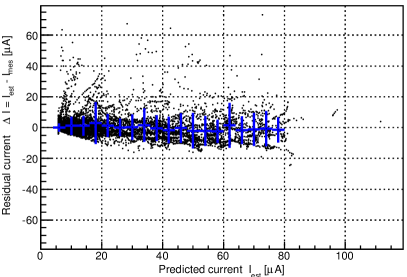
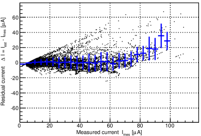
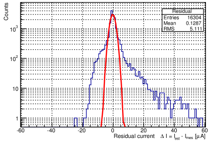
To derive a prediction of the median current in the camera, all physics triggered data taken between 01/09/2013 and 22/07/2014 have been used. Only a single night was excluded due to snow on the ground which significantly increased the background light yield. From these data, relations from the measured current have been derived. Generally, all effects can be described by physical formulas. The disadvantage of such an approach is that instrumental effects like the angular acceptance of the light guides are not included and need additional components. It is unclear, if an easy formula can be derived this way. Formulas to describe the brightness of moonlight have been suggested in literature, e.g. [16], but describe the measured current less accurate than the presented empirical model, c.f. [17]. To derive such an empirical model, the residual between the predicted current and the measured current has been used versus the Sun’s zenith distance $\Theta$, the illuminated fraction $f$ of the moon disk, the Moon’s altitude $\alpha$, the Moon’s distance $d$ from the earth relative to its semi-major axis $d_{0}$ = 384,400 km, and the angular separation $\delta$ between the moon position and the pointing direction. The following fit was achieved:

$$I_{est}/\,\mu A=5.7+95.8\cdot\frac{f^{2.73}\cdot\sin^{0.70}\alpha}{(\frac{d}{d_{0}})^{2}}e^{0.77\cos^{4}\delta}+e^{-97.9+105.9\sin^{2}\Theta}$$ (13)

Figure 15: All three plots show the residual between the predicted current and the measured current. The left plot shows the distribution. The majority of the data is well predictable, presumably the data with good quality. The tails on both sides correspond to non ideal observations conditions. Enhanced current is due to scattering and reflection, while reduced currents are due to attenuation. The fit of a Gaussian yields a sigma of $\sim$1.6 $\mu$A. The central plot shows the residual as a function of the predicted current overlaid with a profile (blue) which error bars denote the standard deviation of the distribution. No significant structure is visible. The right plot is compiled as the central plot but shows the residual versus the measured current. An overestimation of high currents is visible.

Result

In figure 15, the distribution of residuals between the resulting prediction and the measured currents are shown. While the majority of the data shows a residual of less than $\pm$5 $\mu$A, higher residuals are visible originating from attenuation, increased scattering or reflections. For high currents, the prediction is usually overestimating the measured current which is an effect of the exponential increase of light when the Sun is just below the horizon.

While in the above formula some dependencies are easy to fit, such as the dependency of the moon brightness, others like the dependency on sun brightness and angular separation are difficult because of very limited statistics. An additional complication is that in case of the Sun, already small changes in atmospheric scattering imply significant changes in absolute light flux. Due to the exponential behavior, this limits the quality of a simple prediction. This can be verified with the data which shows a significant increase of background light towards sunset and sunrise even during dark time, so called zodiacal light.

Figure 16: The five plots show the average median current (black) per run (5 min) versus time (UTC) compared to the corresponding current prediction (blue) for the nights 26/10/2013, 12/11/2013, 11/01/2014, 12/01/2014 and 13/01/2014 (top to bottom) with a maximum illuminated fraction of the moon disk of roughly 47%, 73%, 84%, 91% and 96% respectively. Poor weather conditions like high humidity and clouds can be seen as short time variation. Smooth variations on longer time scales are assumed to be an effect from reflections. Generally, a good agreement is visible.

In figure 16, some examples are shown, comparing measured and predicted current. The measured current is the median over the camera. The maximum illuminated fraction of the Moon ranges from 47% to 96%. The Moon culminates at a zenith distance of $\sim$10°. Pointing directions are between 10° and 70° zenith distance. The smallest angular distance to the Moon is around 10°.

It is apparent that unexpected events are easy to recognize. While static reflections moving into or out from the field-of-view usually introduce a slow change, reflections from clouds introduce a noise like shape. In other cases, clouds or additional attenuation in the atmosphere show a current drop compared to the prediction. Evaluating this not only visually but also with statistical methods are an ideal tool for data quality checks needed for a stable long term monitoring.

Furthermore, the predicted current is directly related to the energy threshold which can be derived from the trigger threshols, c.f. [18]. This can be used to optimize observation schedule.

7 Conclusions and Outlook

The results presented in this article prove that the FACT camera can be operated under low light conditions with a gain variation of its sensors better than 0.5% on average while providing a homogenous response over the camera of better than 2.5% at the same time. The achieved homogeneity is close to the limit provided by the power supply. This result was derived from measurements of the dark count spectra of the sensors. A special achievement is that for the data analysis, a distribution function, the modified Erlang distribution, was introduced which fits the dark count spectrum even at high multiplicities extremely well. A simple Monte Carlo simulation of the dark count spectrum shows matching results allowing for a proper detector simulation in the data analysis chain. Investigations of the temperature and voltage dependence of the obtained parameters gave a very valuable overview of the behavior of the sensors under varying conditions. Measurements with an external light pulser proved that this stability is maintained on a few percent level up to the brightest light conditions.

It was demonstrated that measurements during bright moon light (see also [15, 17, 18]) are possible under stable trigger conditions.

For these successes, no external calibration device was needed. Even for monitoring purpose the existing light pulser can be omitted because a decrease of sensor properties taking place only at bright light conditions, is not very likely and can therefore be monitored with the dark count spectra. It turned out that a very detailed characterization of the sensors in a laboratory is not necessary and can be done measuring their dark count spectra under varying conditions in the field.

The excellent stability of the gain in space and time also demonstrates that for the existing system the precision of the gain is ultimately limited only by the resolution of the voltage setting. It can be assumed that a more precise voltage supply and knowledge of the voltage applied to the sensor itself can further improve the stability. On the other hand, the presented results show that a power supply which needs to achieve a precision better than 0.5‰ at voltages above 70 V needs a very careful design or detailed characterization especially to avoid any temperature gradients. When several sensors share the same support voltage, it is essential that they are carefully selected in advance, even more if thousands are used. In any case a power supply must be designed to provide currents in the order of a hundred to several hundred $\mu$A per channel if the sensors should be operated during bright light conditions.

In the new generation of G-APDs appearing on the market, most of their features are improved. A new material for the internal quenching resistor reduces the temperature gradient which lowers the requirement for the precision of the temperature measurement and voltage setting. Higher purity of the silicon facilitates a reduction of dark counts and afterpulses. The application of trenches between G-APD cells allows to order sensors with reduced optical crosstalk with the drawback of a reduced active area. Allowing for the same level of crosstalk as in recent sensors, the applied voltage can be increased operating the sensor in a regime in which photo-detection efficiency shows a weaker dependence on temperature and is close to saturation. Through-Silicon Via technology allows to tile several sensors together with almost no gap in between, but also for the price of a small decrease in active area.

This study has impressively proven that even sensors which have been on the market already for several years can be used with high precision for photo detection in cameras even when operated under varying environmental conditions. Regular operations during bright moon light without any hint for decreasing performance since assembly have proven the durability of G-APDs. Although, several hardware failures happened during 2013, as a leaking pump, a blown professional power supply and a broken lid actuator, not a single problem was related to the sensors themselves.

Future projects will strongly benefit from this experience. Already today, several sub projects within the Cherenkov Telescope Array (CTA) project are developing new G-APD based cameras. For a project which is going to operate about one hundred telescopes, especially their stability will lower maintanance costs. The discussed improvements in technology will simplify their application further and at the same improve the achieved performance and consequently simpify data analysis. The very stable operation facilitates an analysis threshold closer to the trigger.

Appendix A The distribution function for the dark count spectrum

A.1 The distribution function

To fit the dark count spectrum measured from a G-APD sensor, a proper distribution function has to be used. The distribution function describes the probability to measure a charge which corresponds to $N$ times the charge released by a single breakdown as a function of $N$. In the following, several distribution functions which come into question are presented and discussed. Some of them have been rearranged to emphasize their common basis.

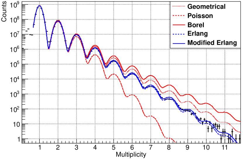
In figure 17, example fits to existing data for the distributions discussed in the following are shown.

Figure 17: A measured single-p.e. spectrum overlayed with several different distribution function fitted to the data. The pure Poisson distribution significantly underestimates the data, while the Borel distribution clearly overestimates the data. The geometrical distribution by chance gets very close to the data. A good fit is obtained by the Erlang and modified Erlang distribution.

Geometric distribution

The most simple distribution function is the geometric distribution. It describes the probability to measure $N$ breakdowns in total, if every breakdown introduces a maximum of one additional breakdown, each with a probability $p$

$$P(N)=p^{N}(1-p)\propto p^{N-1}$$ (14)

$$\Rightarrow\frac{P(N+1)}{P(N)}=p$$ (15)

Poisson distribution

In reality, every avalanche emits several photons which can initiate an additional number $p$ of breakdowns on average. Such a process is described by a Poisson distribution.

$$P(N)=\frac{p^{N}}{N!}e^{-p}\propto\frac{p^{N-1}}{N!}$$ (16)

$$\Rightarrow\frac{P(N+1)}{P(N)}=\frac{p}{N}$$ (17)

Conway-Maxwell-Poisson distribution (CMP)

A generalization of the geometrical and the Poisson distribution is the Conway-Maxwell-Poisson distribution which has the Poisson distribution and the Geometric distribution as special cases. An additional parameter $\nu$ describes a decrease in the probability for successive breakdowns.

$$P(N)\propto\frac{p^{N-1}}{(N!)^{\nu}}$$ (18)

$$\Rightarrow\frac{P(N+1)}{P(N)}=\frac{p}{N^{\nu}}$$ (19)

Borel distribution

In all previous cases, the fact that every secondary avalanche can induce further avalanches is neglected. The absence of branching in the process results in a significant underestimation of the probability for high multiplicities $N$. Including the possibility of branching yields the so-called Borel distribution. It describes the probability to have exactly $N$ breakdowns if every induced avalanche induces a number of independent additional breakdowns and each of these processes is Poisson distributed. If the process is started with more than a single synchronous breakdown, the Borel distribution can be extended to the Borel-Tanner distribution, which is mentioned here only for completeness.

$$P(N)=\frac{1}{N}\frac{(pN)^{N-1}}{(N-1)!}e^{-pN}\propto\frac{1}{N}\frac{(qN)^{N-1}}{(N-1)!}\qquad\mbox{with}\qquad q=pe^{-p}$$ (20)

$$\Rightarrow\frac{P(N+1)}{P(N)}=q\left(\frac{N+1}{N}\right)^{N-1}$$ (21)

For high multiplicities $N$ this ratio converges to $qe$.

For sensors, in which each generation is nearly independent from the previous generation, this description is already fully sufficient as shown in [19], although here, a mismatch at higher orders is visible. In the case of the sensors applied in the FACT camera, it turns out that the Borel distribution overestimates the probability for high multiplicities. Empirically, it has been found that by adding an arbitrary factor $N$, a much better agreement between the probability function and the measured data is obtained.

For geometrical reasons, in general, consecutive generation are not indepent and the number of newly triggered cells is decreasing on average. In every sensor, each cell has only a limited number of neighboring cells which can be triggered and in addition, each cell can be triggered only once. Therefore, it is not expected that the Borel distribution is matching generally.

The emperically obtained distribution is known in the literature as Erlang distribution.

Erlang distribution

The Erlang distribution describes the probability to have exactly $N$ breakdowns in case each breakdown produces $k$ independent breakdowns, each exponentially distributed.

$$P(N,k)=\frac{p^{k}N^{k-1}}{(k-1)!}e^{-pN}$$ (22)

for $k=N$ this yields

$$P(N)\propto\frac{(qN)^{N-1}}{(N-1)!}\qquad\mbox{with}\qquad q=pe^{-p}$$ (23)

$$\Rightarrow\frac{P(N+1)}{P(N)}=q\left(\frac{N+1}{N}\right)^{N}$$ (24)

In the Erlang distribution the ratio between two consecutive probabilities is larger by a factor proportional to $1+1/N$ as compared to the Borel distribution. For high multiplicities $N$, this ratio also converges towards $qe$.

All mentioned distributions describe either a single process, or an infinite chain of processes. Due to the fact that the number of cells in a sensor which can discharge is limited, it turns out that a minor correction for a proper description for multiplicities above $N\approx 7$ is necessary.

The modified Erlang distribution

In analogy to the Conway-Maxwell-Poisson distribution a modified Erlang distribution is introduced, which allows a change of probability with an increasing number of breakdowns. A possible explanation for this small correction is the limited size of the sensor or different crosstalk probabilities of different cells, c.f. [9, 20].

$$P(N)\propto\frac{(qN)^{N-1}}{[(N-1)!]^{\nu}}\qquad\mbox{with}\qquad q=pe^{-p}$$ (25)

$$\Rightarrow\frac{P(N+1)}{P(N)}=\frac{q}{N^{\nu-1}}\left(\frac{N+1}{N}\right)^{N}$$ (26)

For $\nu=1$ this distribution transforms into the standard Erlang distribution.

Approximation

For an easy comparison, the Sterling approximation $N!\approx\sqrt{2\pi N}(N/e)^{N}$ can be applied. For the modified Erlang distribution this yields

$$P(N)\propto\frac{q^{N-1}}{N^{0.5\nu+(N-1)(1-\nu)}}\qquad\mbox{with}\qquad q=pe^{-p\nu}$$ (27)

For $\nu$ very close to unity, the function can be further simplified into

$$P(N)\propto\frac{q^{N-1}}{\left.\sqrt{N}\right.^{\nu}}$$ (28)

$$\frac{P(N+1)}{P(N)}=q\left.\sqrt{\frac{N}{N+1}}\right.^{\nu}$$ (29)

The similarity with the Conway-Maxwell-Poisson distribution is immediately apparent, which fits the dark count spectrum equally well with $\nu\approx 0.5$.

Discussion

In the limit of high multiplicities $N$, the ratio between two consecutive peaks converges to $qe$ for the Borel distribution and the Erlang distribution. At the same time, the ratio of the first two peaks in the Borel distribution is $q$ and in the Erlang distribution $2q$. While in the case of the Borel distribution the deviation from a geometric distribution is obvious, the change in slope for consecutive multiplicities $N$ and $N+1$ decreases from 10% for $N$ = 1 to only 3% for $N$ = 3. Therefore, the resulting distribution can easily be confused with the geometrical distribution if the measurement is not sufficiently sensitive, c.f. figure 17.

A.2 Simulation

Figure 18: Left: Simulation of a simple branching Poisson process (black), i.e. the probability for a successful crosstalk induced breakdown does not change and a fit of the corresponding Borel distribution; and the simulation of a Poisson process which takes the geometry of the sensor into account (blue) and a fit of the corresponding modified Erlang distirbution. Right: Data fitted with an Erlang distribution (dashed line) and a modified Erlang distribution (solid line). Superimposed is a geometry aware simulation using the properly converted fit parameters as input. Each red dot corresponds to the amplitude of a Gaussian with noise parameters as obtained from the fit. A good match between the simulated process and the original distribution is visible.

Figure 19: Erlang distribution for crosstalk probabilities of 5%, 10%, 15%, 20% and 30%. The crosstalk probability is the number of of breakdowns with $N>1$ divided by the total number of breakdowns.

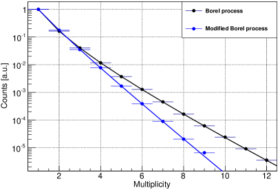
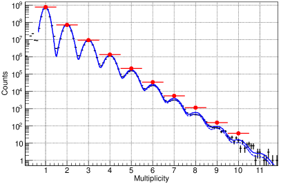
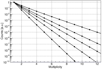
Although a distribution function has been found empirically which fits the measured dark count spectra extremely well, its understanding is essential for a proper detector simulation.

To initially understand the empirical modification on the Borel-distribution, at first, an ideal Borel distribution has been simulated.

Branching Poisson process (Borel-distribution)

In the Borel process, each breakdown creates further breakdowns with identical Poisson distributions. The following recursive code snippet returns a random number of total breakdowns including the primary breakdown.

int hit()
{
    int n = random_poisson(probability);
    int counter=1;
    for (int i=0; i<n; i++)
        counter += hit();
    return counter;
}

The result for a Poisson probability of 20% is shown in figure 18 (left) in black. Superimposed is a fit of a Borel distribution. As expected, simulation and fit show a good agreement. The fit yields a probability $p$ within errors consistent with 0.2.

Branching Poisson process with geometry awareness

For the simulated Borel process it is assumed that each branching process takes place with identical probabilities. Considering a real crosstalk process on a sensor, it would mean that the emitted photons always have exactly the same probability to induce further breakdowns. While the number of emitted photons is Poisson distributed, the number of charged cells in the direct vicinity of the emitting cell is decreasing with each discharge. The requirement that only direct neighboring cells can suffer a breakdown effectively limits the number of crosstalk induced discharges to four. This geometrical effect has to be taken into account in the simulation. In addition, it must be considered that a real sensor has only a finite number of available cells in total. Therefore, a realistic simulation has to take the geometry into account and memorize discharged cells. An implementation for a quadratic device with 3600 cells is shown in the following code snippet, assuming that crosstalk only affects direct neighbors. The returned value is the random number of total breakdowns induced including the primary breakdown.

int hit(int x, int y)
{
    if (not_inside(x, y) || is_discharged(x, y))
        return 0;
    discharge(x, y);
    int n = random_poisson(probability);
    int counter = 1;
    for (int i=0; i<n; i++)
    {
        switch (random_direction())
        {
        case 0: counter += hit(x+1, y); break;
        case 1: counter += hit(x-1, y); break;
        case 2: counter += hit(x, y+1); break;
        case 3: counter += hit(x, y-1); break;
        }
    }
    return counter;
}

The result of this simulation for a probability of 20% is shown in figure 18 (left) in blue. Superimposed is a fit of a modified Erlang distribution as introduced earlier. Simulation and fit show a good match. The fit yields the following results:

$$p=0.2196\pm 0.0002$$ (30)

$$\nu=0.978\pm 0.002$$ (31)

Figure 20: The probability $p$ (left, blue) and the exponent $\nu$ (right) of the a fit of a modified Erlang distribution versus the Poisson probability $p$ of a simulation taking the geometry into account. The black dots show the corresponding crosstalk probability $p_{xt}$. Both probabilities are superimposed with a fit of the form $c_{0}p^{c_{1}}$. The right curve was fitted with $(cp+1)/(p+1)$.

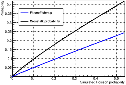
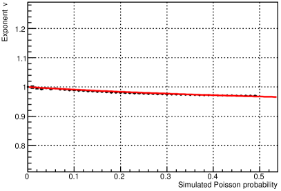
By changing the simulated probability, no decrease in the fit quality is observed. It also allows to find a relation between the Poisson probability $p$ in the simulation and the coefficient $p_{fit}$ of the fit of an Erlang distribution, the crosstalk probability $p_{xt}$ and the exponent $\nu$. The result is shown in figure 20. The fits yield

$$p_{fit}=(0.440106\pm 0.00010)\cdot p^{0.9515\pm 0.0020}$$ (32)

$$p_{xt}=(0.723\pm 0.004)\cdot p^{0.875\pm 0.005}$$ (33)

$$\nu=\frac{(0.902387\pm 0.00006)\cdot p+1}{p+1}$$ (34)

These relations can be used to estimate the probability $p$ needed for the simulation from a fit to the data. More precise fits can be found, but for the simulation a higher precision is not necessary.

So far, the possibility that a crosstalk photon induces a breakdown in another cell other than a direct neighbor has still been neglected. This can be taken into account if photons are simulated with a distribution which is exponentially falling from the center of the emitting cell and uniform in direction. Since this effect is only visible for $N>10$, it is negligible for image reconstruction in Cherenkov astronomy and only relevant if exact rate for high thresholds need to be calculated.

A.3 Application

In figure 18 (right) the measured data superimposed with a fit of an ideal Erlang distribution (solid line) and a modified Erlang distribution (dashed line) are shown. Superimposed (red dots) is a simulation with Poisson probability $p$ obtained from the parameter $p_{fit}$ from a fit of a modified Erlang distirbution. It can be seen that a good match with the ideal Erlang distribution is obtained.

Knowing the proper distribution function also allows to compare the influence of the crosstalk probability on the distribution. Figure 19 shows the expected distribution for different crosstalk probabilities.

A.4 Result

The spatial compactness of successive breakdowns in crosstalk events has a strong influence on the distribution. This influence is described well by a slightly modified Erlang distribution. The additional factor $N$ by which the Erlang distribution deviates from the Borel distribution can be interpreted as the loss of charged cells in the vicinity of the avalanche emitting photons. The exponent $\nu$ can be interpreted as a further fine tuning of the geometrical behavior, for example, the probability that non direct neighbors are triggered. That the Erlang distribution yields reasonable results can be interpreted such that each breakdown induces additional breakdowns with an exponential distribution due to the loss of available charged cells with increasing number.