Effect of electron-phonon interactions on Raman line at ferromagnetic ordering

Abstract

The theory of Raman scattering in half-metals by optical phonons interacting with conduction electrons is developed. We evaluate the effect of electron-phonon interactions at ferromagnetic ordering in terms of the Boltzmann equation for carriers. The chemical potential is found to decrease with temperature decreasing. Both the linewidth and frequency shift exhibit a dependence on temperature.

I Introduction

Recently, the Raman scattering in the half-metallic CoS₂ was studied La in the wide temperature region. The $\omega=400$ cm^-1 Raman line, observed previously at room temperature in Ref. AP ; ZST , demonstrates a particular behavior nearby the ferromagnetic transition at $T_{c}=122$ K. The unusual large Raman linewidth and shift of the order of 10 cm^-1 were observed. The reflectivity singularities of CoS₂ were explained in Ref. YMM by the temperature variation of the electronic structure. Another example of the electron-phonon interactions is given in Ref. LM in order to explain the phonon singularity at the $\Gamma$ point in graphene. The electron-phonon interactions should be considered as well in the interpretation of the observed Raman scattering around the Curie temperature.

Thermal broadening of phonon lines in the Raman scattering is usually described in terms of three-phonon anharmonicity, i.e. by the decay of an optical phonon with a frequency $\omega$ in two phonons. The simplest case when the final state has two acoustic phonon from one branch (the Klemens channel) was theoretically studied by Klemens Kl , who obtained the temperature dependence of the Raman linewidth. The corresponding lineshift was considered in Refs. BWH ; MC . This theory was compared in works BWH ; MC ; DBM with experimental data for Si, Ge, C, $\alpha-$Sn. A model was also considered with the phonons in the final state from different branches. It was found that anharmonic interactions of the forth order should be disregarded at high temperatures $T>300$ K.

The situation is more complicated in substances with magnetic ordering. The interaction of phonons with magnons in antiferromagnets was discussed in the review article GZ and more recently in the analysis of the thermal conductivity MOZ , the spin Seebeck effect UTH ; JYM , high-temperature superconductivity NMH , and optical spectra KKP . The magnon-phonon interaction results in the magnon damping Wo , however, no effect for phonons was observed. The influence of antiferromagnetic ordering is considered in Ref. DPV , where the line shift was only calculated. Damping of the optical phonons was found MPB to become large in the rare-earth Gd and Tb below the Curie temperature achieving a value of 15 cm^-1, which is much greater than the three-phonon interaction effect.

Despite attracting considerable interest for half a century since the pioneering work by Fröhlich, the problem of electron-phonon interaction is still far from being solved. Migdal Mi developed a consistent many-body approach based on the Fröhlich Hamiltonian for interaction of electrons with acoustic (sound) phonons. As Migdal showed (”the Migdal theorem”), the vertex corrections for acoustic phonons are small by the adiabatic parameter $\sqrt{m/M}$, where $m$ and $M$ are the electron and ion masses, respectively. The theory described correctly the electronic lifetime, renormalization of the Fermi velocity $v_{F}$ and acoustic phonon attenuation but resulted in a strong renormalization of the sound velocity $\tilde{s}=s(1-2\lambda)^{1/2}$, where $\lambda$ is the dimensionless coupling constant. For sufficiently strong electron-phonon coupling $\lambda\to 1/2$, the phonon frequency approached to zero marking an instability point of the system. Instead, one would intuitively expect the phonon renormalization to be weak along with the adiabatic parameter.

This discrepancy was resolved by Brovman and Kagan BK almost a decade later (see also G ). They demonstrated the shortcomings of the Fröhlich model that gave an anomalously large phonon renormalization. Employing the Born–Oppenheimer (adiabatic) approximation (see, e.g., BHK ), they found that there are two terms in the second order perturbation theory, which compensate each other making a result small by the adiabatic parameter. Namely, when calculating the phonon self-energy function $\Pi(\omega,k)$ with help of the diagram technique, one should eliminate an adiabatic contribution of the Fröhlich model by subtracting $\Pi(\omega,k)-\Pi(0,k)$.

The interaction of electrons with optical phonons was first considered by Engelsberg and Schrieffer ES within Migdal’s many-body approach for dispersionless phonons. They predicted a splitting of the optical phonon at finite wavenumbers $k$ into two branches. Ipatova and Subashiev IS calculated later on the optical phonon attenuation in the collisionless limit and pointed out that the Brovman-Kagan renormalization should be carried out for optical phonons in order to obtain correct phonon renormalization. In the paper AS , Alexandrov and Schrieffer corrected the calculational error of Ref. ES and argued that no splitting was found in fact. Instead, they predicted an extremely strong dispersion of optical phonons, $\omega_{k}=\omega_{0}+\lambda v_{F}^{2}k^{2}/3\omega_{0}$, due to the coupling to electrons. The large phonon dispersion is a typical result of Migdal’s theory AGD using the Frölich Hamiltonian. No such a dispersion has ever been observed experimentally. The usual dispersion of optical phonons in metals has the order of the sound velocity. Reizer R stressed the importance of screening effects which should be taken into account. The works AS ; R are limited to the case of collisionless both electron and phonon systems. Moreover, only the phonon renormalization was considered with no results available for the attenuation of optical phonons.

A different from many-body technique semiclassical approach based on the Boltzmann equation and the equations of the theory of elasticity was developed in the papers by Akhiezer, Silin, Gurevich, Kontorovich, and many others (we refer the reader to the review Kon ). This approach was compared with various experiments, such as attenuation of sound waves, effects of strong magnetic fields, crystal anisotropy, and sample surfaces on the sound attenuation, and so on. It can be applied to the problem of the electron–optical-phonon interaction MF as well.

In the previous paper Fal , we have developed a quantum theory for the optical phonon attenuation and shift induced by the interband electron transitions and tuned with a temperature variation. Now we consider the optical phonon renormalization as a result of the electron-phonon interaction taking into account ferro-magnetic ordering. We argue that the reasonable phonon damping and shift can be obtained using the semiclassical Boltzmann equation for electrons and the motion equation of phonons coupled by the deformation potential.

II Electron-phonon interactions at ferromagnetic ordering

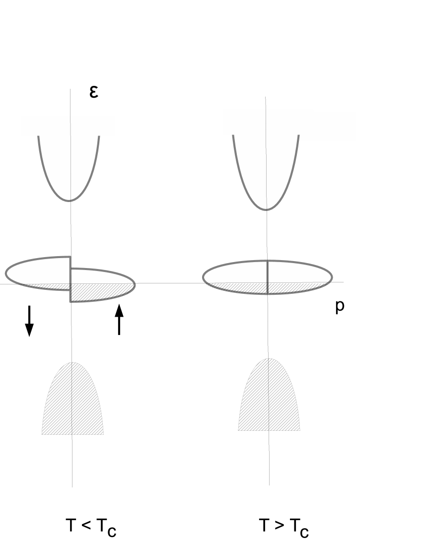
Figure 1: (Color online) Proposed band scheme for two electron spin projections.

We assume that the electron bands in CoS₂ have a form shown in Fig. 1. The ferromagnetic ordering results in the spin splitting $\mu H_{e}$ of the unfilled half-metallic band

$$\begin{array}[]{c}\displaystyle{\varepsilon_{\uparrow}({\bf p})=\frac{p^{2}}{2m^{\vee}}}-\mu H_{e}\quad\text{and}\quad\displaystyle{\varepsilon_{\downarrow}({\bf p})=\frac{p^{2}}{2m^{\vee}}}+\mu H_{e}\end{array}$$ (1)

in the effective Weiss field $H_{e}$. While the temperature decreases, the magnetization, determined in the mean field approximation as

$$M=M_{0}\sqrt{1-(T/T_{c})^{2}}\,,$$ (2)

appears according to experimental data in CoS₂ at $T_{c}=122$ K approximately, and the spin splitting is proportional to the magnetization.

We write the interaction of electrons with the optical phonon $u_{i}$ as the deformation potential

$$H_{int}=\frac{u_{i}}{N}\sum_{s}\int\frac{d^{3}{\bf p}}{(2\pi\hbar)^{3}}\zeta_{i}({\bf p})f({\bf p})\,,$$ (3)

where $N\sim 1/a^{3}$ is a number of cells in the volume unit and $a$ is the interatomic distance. For the acoustic phonon – electron interaction, we should substitute the strain tensor $u_{ij}$ instead of the displacement $u_{i}$ in order to satisfy the translation symmetry of the lattice.

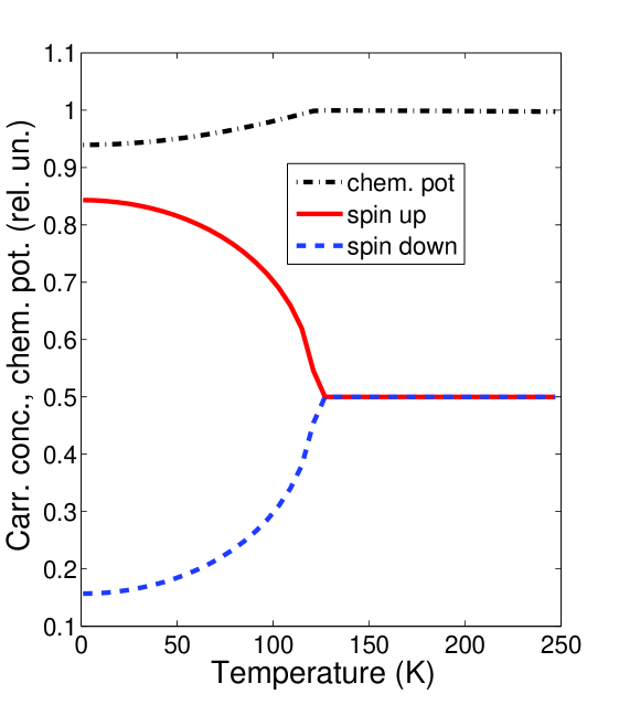
Figure 2: (Color online) Calculated temperature dependence of the carrier concentration for the spin up and spin down (relative to the total concentration at temperatures above the temperature of ferromagnetic ordering), and the dependence of the chemical potential (dash-dotted line).

The Boltzmann equation for the nonequilibrium part of the distribution function $f({\bf p})$ has the form

$$[-i(\omega-{\bf k\cdot v})+\tau^{-1}]f({\bf p})=-\frac{\partial f_{0}}{\partial\varepsilon}[e{\bf v\cdot E}-i\omega u_{i}\zeta_{i}({\bf p})]\,,$$ (4)

where $f_{0}$ is the equilibrium distribution function. We omit in the Boltzmann equation (4) the spin index $s$, which determines all the electron parameters. The electron collision frequency $\tau^{-1}$ takes into account the collisions with impurities and phonons. The collision frequency is calculated for CoS₂ in the Debye model with the temperature $T_{D}=500$ K. One can see from Eq.(4) that the condition

$$<\zeta_{i}>=0\,,$$

have to be satisfied in order to obey the current continuity equation, where the brackets mean averaging over the Fermi surface for temperatures $T\ll\varepsilon_{F}$.

In the ferromagnetic phase while the temperature changes, the carriers overflow from one spin state in another, but the total number of carriers

$$N=\sum_{s}\int\frac{d^{3}{\bf p}}{(2\pi\hbar)^{3}}f_{0}(\varepsilon_{s})$$ (5)

remains to be constant. This condition determines the chemical potential and the carrier concentration with the spin up and spin down, shown in Fig.2. All figures correspond here and what follows to the carrier concentration $N=10^{21}$ cm^-3 in the considered band with the Fermi energy $\mu=0.36$ eV above the Curie temperature.

Let us write the motion equation for the phonon mode in a form

$$(\omega_{0}^{2}-\omega^{2})u_{i}=\frac{QE_{i}}{M}-\frac{1}{M}\frac{\partial H_{int}}{\partial u_{i}}\,,$$ (6)

where $M$ is the reduced ion mass of the cell, $Q$ is the charge corresponding to the optical vibration, and $\omega_{0}$ is the frequency of the considered mode. Here, the last term represents the electron-phonon interaction. Using the Boltzmann equation (4), we rewrite this term as follows

$$-\frac{1}{M}\frac{\partial H_{int}}{\partial u_{i}}=-\frac{u_{i}}{MN}\sum_{s}\int\frac{\omega\tau\zeta^{2}_{i}({\bf p})}{\omega\tau+i}\left(-\frac{\partial f_{0}}{\partial\varepsilon}\right)\frac{d^{3}{\bf p}}{(2\pi\hbar)^{3}}\,.$$ (7)

The term with electric field in the Boltzmann equation disappears in the integration over ${\bf p}$ due to the velocity inversion ${\bf v}\rightarrow-{\bf v}$. The term with the wave vector ${\bf k}$ has to be omitted for the Raman phonon, as the vector ${\bf k}$ is determined in this case by the laser frequency $\omega_{i}$ and the optical phonon frequency satisfies the condition $\omega\gg\omega_{i}v/c$.

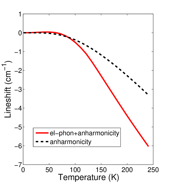
Figure 3: (Color online) Calculated shift of the Raman line $\omega=400$ cm^-1 due to the electron-phonon interaction, and the lineshift in the Klemens channel (dashed line).

The electric field does not excited in the TO vibrations. Therefore, supposing $E=0$ and integrating over the energy $\varepsilon$ instead of $p$, we find from Eqs. (6) and (7) the lineshift $\delta\omega$ and linewidth $\delta\Gamma$ determined by the electron-phonon interaction as

$$\delta\omega_{TO}-i\delta\Gamma_{TO}=\frac{1}{2MN}\sum_{s}\int\frac{\tau(\omega\tau-i)\zeta^{2}({\bf p})dS}{(\omega^{2}\tau^{2}+1)v(2\pi\hbar)^{3}}|_{\varepsilon=\varepsilon_{F}}\,,$$ (8)

where $dS$ is an element of the Fermi surface, $v$ is the Fermi velocity. Estimating $S=4\pi p_{F}^{2}$, $\zeta({\bf p})\sim\varepsilon_{0}/a$ and $\varepsilon_{0}^{2}\sim\omega^{2}M/m$, where $\varepsilon_{0}\sim 3eV$ is the typical electron energy in metals, we obtain

$$\delta\omega_{TO}-i\delta\Gamma_{TO}\sim\frac{ap_{F}\tau\omega^{2}_{TO}}{2\pi^{2}\hbar(\tau\omega_{TO}+i)}\,.$$

The equations (6) and (7) allow to express the phonon displacement $u$ in terms the electric field $E$ and to calculate the phonon contribution $uNQ$ into the polarization. We find the total dielectric permittivity, adding the contributions $\varepsilon_{\infty}$ of the filled bands

$$\begin{array}[]{c}\varepsilon(\omega)={\displaystyle\varepsilon_{\infty}-\frac{4\pi e^{2}}{3\omega}\sum_{s}\int\frac{\tau vdS}{(\omega\tau+i)(2\pi\hbar)^{3}}}+\\ {\displaystyle\frac{4\pi NQ^{2}}{M}\left[\omega_{0}^{2}-\omega^{2}+\frac{\omega\tau}{MN}\sum_{s}\int\frac{\zeta^{2}({\bf p})dS}{(\omega\tau+i)v(2\pi\hbar)^{3}}\right]^{-1}}.\end{array}$$ (9)

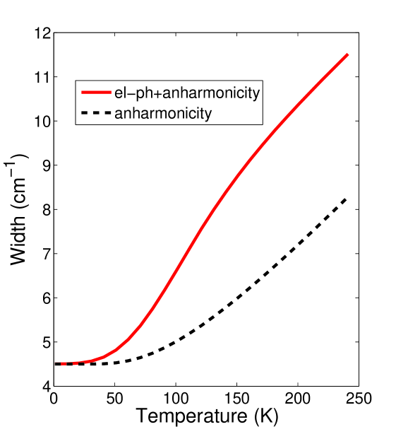
Figure 4: (Color online) Calculated temperature dependence of the width for the Raman $\omega=400$ cm^-1 line at the ferromagnetic ordering, and the linewidth in the Klemens channel (dashed line).

The frequency of the longitudinal phonon mode is determined by the condition $\varepsilon(\omega)=0$. In the absence of free carriers, one finds the frequency of the LO mode as follows

$$\omega_{LO}^{2}=\omega_{0}^{2}+\omega_{pi}^{2},$$

where $\omega_{pi}^{2}=4\pi NQ^{2}/M\varepsilon_{\infty}$ is the ion plasma frequency squared.

Using Eq. (9), we find the LO frequency in the presence of carriers as

$$\omega^{2}_{LO}-\omega_{0}^{2}=\frac{\omega}{(2\pi\hbar)^{3}MN}\sum_{s}\int\frac{\tau\zeta^{2}({\bf p})dS}{(\omega\tau+i)v}-\frac{\omega_{pi}^{2}}{\omega_{pe}^{2}}\omega(\omega+i\tau^{-1})\,,$$ (10)

where the electron plasma frequencies squared

$$\omega_{pe}^{2}=\frac{4\pi e^{2}}{3\varepsilon_{\infty}}\sum_{s}\int\frac{vdS}{(2\pi\hbar)^{3}}\,$$ (11)

is supposed to be large in comparison with $\omega_{pi}^{2}$. We can put also $\omega=\omega_{LO}$ in the right-hand side of Eq. (10). Here the last term describes the electric field screened by the free carriers. The main role plays the first term, which coincides with the result for the TO mode, Eq. (8), shown in Figs. 3 and 4, the results for the Klemens channel are taken from Ref. Fal .

We should emphasize that the temperature dependence of the linewidth and shift, Eq. (8), is determined mainly by the electron collision rate $\tau^{-1}$ involving also, for instance, in the dc conductivity. Thus, for a cubic crystal, the dc conductivity, i.e. at $\omega=k=0$, writes

$$\sigma=\sum_{s}\frac{e^{2}}{3(2\pi\hbar)^{3}}\int\tau vdS\,.$$

The details of the electron density of states and of the deformation potential are responsible for peculiarities of the Raman line temperature dependence.

III summary

The Klemens formula describes the optical phonon width due to three-phonon anharmonic interactions. The corresponding lineshift matches with the linewidth. In such ferromagnets as CoS₂ with the low Curie temperature, these interactions are found to be too weak to describe quantitatively the experimental data and to explain the very large Raman linewidth and shift. Therefore, we propose the mechanism of the electron-phonon interaction attended with the effect of the ferromagnetic ordering on the electron bands. The deformation potential couples together the Boltzmann equation for electrons and the motion equation for phonons producing the renormalization of the phonon frequency. The corresponding Raman line width and shift are in agreement with experiments in Ref. La .

IV acknowledgments

The author thank S. Lyapin and S. Stishov for information on their experiments prior the publication, and A. Varlamov for useful discussions. This work was supported by the Russian Foundation for Basic Research (grant No. 13-02-00244A) and the SIMTECH Program, New Centure of Superconductivity: Ideas, Materials and Technologies (grant No. 246937).

References

- (1) S.G. Lyapin, A.N. Utyuzh, A.E. Petrova, A.P. Novikov, T.A. Lograsso, and S.M. Stishov, arXiv:1402.5785.
- (2) E. Anastassakis and C. Perry, J. Chem. Phys. 64, 3604 (1976).
- (3) L. Zhu, D. Susac, M. Teo, K.C. Wong, P.C. Wong, R.R. Parsons, D. Bizzotto, K.A.R. Mitchel, and S.A. Campbell, J. Catal. 258, 235 (2008).
- (4) R. Yamamoto, A. Machida, Y. Moritomo, and A. Nakamura, Phys. Rev. B 59, R7793 (1999).
- (5) S. Piscanec, M. Lazzeri, Francesco Mauri, A.C. Ferrari, and J. Robertson, Phys. Rev. Lett. 93, 185503 (2004); M. Lazzeri, S. Piscanec, Francesco Mauri, A.C. Ferrari, and J. Robertson, Phys. Rev. B 73, 155426 (2006); M. Lazzeri and Francesco Mauri, Phys. Rev. Lett. 97, 266407 (2006).
- (6) P.G. Klemens, Phys. Rev. 148, 845 (1966).
- (7) M. Balkanski, R.F. Wallis, and E. Haro, Phys. Rev. B 28, 1928 (1983).
- (8) J. Menéndez and M. Cardona, Phys. Rev. B 29, 2051 (1984).
- (9) A. Debernardi, S. Baroni, and E. Molinari, Phys. Rev. Lett. 75, 1819 (1995).
- (10) G. Güntherodt and R. Zeyer, Light Scattering in Solids, vol. 4 (1984).
- (11) M. Montagnese, M. Otter, X. Zotos, D.A. Fishman, N. Hlubek, O. Mityashkin, C. Hess, R. Saint-Martin, S. Singh, A. Revcolevschi, and P.H.M. van Loosdrecht, Phys. Rev. Lett. 110, 147206 (2013).
- (12) S. Uchida, S. Takahashi, K. Harri, J. Ieda, W. Koshibae, K. Ando, S. Maekawa, and E. Saitoh, Nature (London) 455, 778 (2008).
- (13) C.M. Jaworski, J. Yang, S. Mack, D.D. Awschalom, R.C. Myers, and J.R. Heremans, Phys. Rev. Lett. 106, 186601 (2011).
- (14) F. Nori, R. Merlin, S. Haas, A. Sandvik, and E. Dagotto, Phys. Rev. Lett. 75, 553 (1995).
- (15) S.A. Klimin, A.B. Kuzmenko, M.N. Popova, B.Z. Malkin, and I.V. Telegina, Phys. Rev. B 82, 174425 (2010).
- (16) L.M. Woods, Phys. Rev. B 65, 014409 (2001).
- (17) D.M. Djokic, Z.V. Popovic, F.R. Vukajlovic, Phys. Rev. B 77, 014305 (2008).
- (18) A. Melnikov, A. Povolotskiy, and U. Bovensiepen, Phys. Rev. Lett. 100, 247401 (2008).
- (19) A.B. Migdal, Sov. Phys. JETP 7, 996 (1958).
- (20) E.G. Brovman and Yu. Kagan, Sov. Phys. JETP 25, 365 (1967).
- (21) B.T. Geilikman, J. Low Temp. Phys. 4, 189, (1971).
- (22) M. Born and Kung Huang, Dynamical Theory of Crystal Lattices (Oxford University Press, New York, 1954).
- (23) S. Engelsberg and J.R. Schrieffer, Phys. Rev. 131, 993 (1963).
- (24) I.P. Ipatova and A.V. Subashiev, Sov. Phys. JETP 39, 349 (1974).
- (25) A.S. Alexandrov and J.R. Schrieffer, Phys. Rev. B 56, 13731 (1997).
- (26) A.A. Abrikosov, L.P. Gor’kov, and I.Ye. Dzyaloshinskii, Methods of Quantum Field Theory in Statistical Physics, (Prentice-Hall, Englewood Cliffs, NJ, 1963).
- (27) M. Reizer, Phys. Rev. B 61, 40 (2000).
- (28) V.M. Kontorovich, Sov. Phys. Uspekhi 27 (2), 134 (1984).
- (29) L.A. Falkovsky and E.G. Mishchenko, Phys. Rev. B 51, 7239 (1995); L.A. Falkovsky, Phys. Rev. B 66, 020302(R) (2002).
- (30) L.A. Falkovsky, Phys. Rev. B 88, 155135 (2013).