$\varepsilon$-Strong Simulation for Multidimensional Stochastic Differential Equations via Rough Path Analysis

Abstract

Consider a multidimensional diffusion process $X=\{X\left(t\right):t\in[0,1]\}$. Let $\varepsilon>0$ be a deterministic, user defined, tolerance error parameter. Under standard regularity conditions on the drift and diffusion coefficients of $X$, we construct a probability space, supporting both $X$ and an explicit, piecewise constant, fully simulatable process $X_{\varepsilon}$ such that

$$\sup_{0\leq t\leq 1}\left\|X_{\varepsilon}\left(t\right)-X\left(t\right)\right\|_{\infty}<\varepsilon$$

with probability one. Moreover, the user can adaptively choose $\varepsilon^{\prime}\in\left(0,\varepsilon\right)$ so that $X_{\varepsilon^{\prime}}$ (also piecewise constant and fully simulatable) can be constructed conditional on $X_{\varepsilon}$ to ensure an error smaller than $\varepsilon^{\prime}$ with probability one. Our construction requires a detailed study of continuity estimates of the Itô map using Lyons’ theory of rough paths. We approximate the underlying Brownian motion, jointly with the Lévy areas with a deterministic $\varepsilon$ error in the underlying rough path metric.

, and

1 Introduction

Consider the Itô Stochastic Differential Equation (SDE)

$$dX(t)=\mu(X(t))dt+\sigma(X(t))dZ(t)\mbox{ , }X(0)=x(0)$$ (1.1)

where $Z\left(\cdot\right)$ is a $d^{\prime}$-dimensional Brownian motion, and $\mu\left(\cdot\right):R^{d}\rightarrow R^{d}$ and $\sigma\left(\cdot\right):R^{d}\rightarrow R^{d\times d^{\prime}}$ satisfy suitable regularity conditions. We shall assume, in particular, that both $\mu\left(\cdot\right)$ and $\sigma\left(\cdot\right)$ are Lipschitz continuous so that a strong solution to the SDE is guaranteed to exist. Additional assumptions on the first and second order derivatives of $\mu\left(\cdot\right)$ and $\sigma\left(\cdot\right)$, which are standard in the theory of rough paths, will be discussed in the sequel.

Our contribution in this paper is the joint construction of $X=\{X\left(t\right):t\in[0,1]\}$ and a family of processes $X_{\varepsilon}=\{X_{\varepsilon}\left(t\right):t\in[0,1]\}$, for each $\varepsilon\in\left(0,1\right)$, supported on a probability space $\left(\Omega,\mathcal{F},P\right)$, and such that the following properties hold:

1. The process $X_{\varepsilon}$ is piecewise constant, with finitely many discontinuities in $[0,1]$.

2. The process $X_{\varepsilon}$ can be simulated exactly and, since it takes only finitely many values, its path can be fully stored.

3. We have that with $P$-probability one

   $$\sup_{t\in[0,1]}\left|\left|X_{\varepsilon}\left(t\right)-X\left(t\right)\right|\right|_{\infty}<\varepsilon.$$ (1.2)

4. For any $m>1$ and $0<\varepsilon_{m}<...<\varepsilon_{1}<1$ we can simulate $X_{\varepsilon_{m}}$ conditional on $X_{\varepsilon_{1}}$,…,$X_{\varepsilon_{m-1}}$.

We refer to the class of procedures which achieve the construction of such family $\{X_{\varepsilon}:\varepsilon\in\left(0,1\right)\}$ as Tolerance-Enforced Simulation (TES) or $\varepsilon$-strong simulation methods. Throughout the paper we use $||\cdot||_{\infty}$ to denote the max-norm on $\mathbb{R}^{d}$.

This paper provides the first construction of a Tolerance-Enforced Simulation procedure for multidimensional SDEs in substantial generality. All other TES or $\varepsilon$-strong simulation procedures up to now are applicable to one dimensional processes or multidimensional processes with constant diffusion matrix (i.e. $\sigma\left(x\right)=\sigma$).

Let us discuss some considerations that motivate our study. We first discuss how this paper relates to the current literature on $\varepsilon$-strong simulation of stochastic processes, which is a recent area of research. The paper of [6] provides the construction of $X_{\varepsilon}$ satisfying only (T1) to (T3), in one dimension. In particular, bound (1.2) is satisfied for a given fixed $\varepsilon_{0}=\varepsilon>0$ and it is not clear how to jointly simulate $\left\{X_{\varepsilon_{m}}\right\}_{m\geq 1}$ as $\varepsilon_{m}\searrow 0$  applying the technique in [6]. The motivation of constructing $X_{\varepsilon_{0}}$ for [6] came from the desire to produce exact samples from a one dimensional diffusion $X\left(\cdot\right)$ satisfying (1.1), and also assuming $\sigma\left(\cdot\right)$ constant.

The authors in [6] were interested in extending the applicability of an algorithm introduced by Beskos and Roberts, see [2]. The procedure of Beskos and Roberts, applicable to one dimensional diffusions, imposed strong boundedness assumptions on the drift coefficient and its derivative. The technique in [6] enabled an extension which is free of such boundedness assumptions by using a localization technique that allowed to apply the ideas behind the algorithm in [2]; see also [3] for another approach which eliminates boundedness assumptions. All of these developments are in the one-dimensional case.

The assumption of a constant diffusion coefficient comes at basically no cost in generality when considering one dimensional diffusions because one can always apply Lamperti’s (one-to-one) transformation. Such transformation allows to recast the simulation problem to one involving a diffusion with constant $\sigma\left(\cdot\right)$. Lamperti’s transformation cannot be generally applied in higher dimensions.

The paper of [4] extends the work of [6] in that their algorithms satisfy (T1) to (T4), but also in the context of one dimensional processes. The paper [11] not only provides an additional extension which allows to deal with one dimensional SDEs with jumps, but also contains a comprehensive discussion on exact and $\varepsilon$-strong simulation for SDEs. Property (T4) in the definition of TES is desirable because it provides another approach at constructing unbiased estimators for expectations of the form $Ef\left(X\right)$, where $f\left(\cdot\right)$ is, say, a continuous function of the sample path $X$. In order to see this, let us assume for simplicity that $f\left(\cdot\right)$ is positive and Lipschitz continuous in the uniform norm with Lipschitz constant $K$. Then, let $T$ be any positive random variable with a strictly positive density $g\left(\cdot\right)$ on $[0,\infty)$ and define

$$Z:=I\left(f\left(X\right)>T\right)/g\left(T\right).$$ (1.3)

Observe that

$$E[Z]=E[E\left[Z|X\right]]=E\left[\int_{0}^{\infty}I\left(f\left(X\right)>t\right)\frac{g\left(t\right)}{g\left(t\right)}dt\right]=E[f\left(X\right)],$$

so $Z$ is an unbiased estimator for $Ef\left(X\right)$. Therefore, if Properties T(1) to T(4) hold, it is possible to simulate $Z$ by noting that $f\left(X_{\varepsilon}\right)>T+K\varepsilon$ implies $f\left(X\right)>T$ and if $f\left(X_{\varepsilon}\right)<T-K\varepsilon$, then $f\left(X\right)\leq T$. Since (T4) allows to keep simulating as $\varepsilon$ becomes smaller and $T$ is independent of $X_{\varepsilon}$ with a positive density $g\left(\cdot\right)$, then one eventually is able to simulate $Z$ exactly.

The major obstacle involved in developing exact sampling algorithms for multidimensional diffusions is the fact that $\sigma\left(\cdot\right)$ cannot be assumed to be constant. Moreover, even in the case of multidimensional diffusions with constant $\sigma\left(\cdot\right)$, the one dimensional algorithms developed so far can only be extended to the case in which the drift coefficient $\mu\left(\cdot\right)$ is the gradient of some function, that is, if $\mu\left(x\right)=\nabla v\left(x\right)$ for some $v\left(\cdot\right)$. The reason is that in this case one can represent the likelihood ratio $L\left(t\right)$, between the solution to (1.1) and Brownian motion (assuming $\sigma=I$ for simplicity) involving a Riemann integral as follows

$$L\left(t\right) =\exp\left(\int_{0}^{t}\mu\left(X\left(s\right)\right)dX\left(s\right)-\frac{1}{2}\int_{0}^{t}\left\|\mu\left(X\left(s\right)\right)\right\|_{2}^{2}ds\right)$$

$$=\frac{\exp\left(v\left(X\left(t\right)\right)\right)}{\exp\left(v\left(X\left(0\right)\right)\right)}\exp\left(-\frac{1}{2}\int_{0}^{t}\lambda\left(X\left(s\right)\right)ds\right),$$ (1.4)

for $\lambda\left(x\right)=\Delta v\left(x\right)+\left|\left|\nabla v\left(x\right)\right|\right|_{2}^{2}$. The fact that the stochastic integral can be transformed into a Riemann integral facilitates the execution of acceptance-rejection because one can interpret (up to a constant and using localization as in [6]) the exponential of the integral of $\lambda\left(\cdot\right)$ as the probability that no arrivals occur in a Poisson process with a stochastic intensity. Such event (i.e. no arrivals) can be simulated by thinning.

So, our motivation in this paper is to investigate a novel approach that allows to study $\varepsilon$-strong simulation for multidimensional diffusions in substantial generality, without imposing the assumption that $\sigma\left(\cdot\right)$ is constant or that a Lamperti-type transformation can be applied. Given the previous discussion on the connections between exact sampling and $\varepsilon$-strong simulation, and the limitations of the current techniques, we believe that our results here provide an important step in the development of exact sampling algorithms for general multidimensional diffusions. For example, in contrast to existing techniques, which demand $L\left(t\right)$ to be expressed in terms of a Riemann integral as indicated in (1.4), our results here allow to approximate directly $L\left(t\right)$ in terms of the stochastic integral representation (and thus one does not need to assume that $\mu\left(x\right)=$ $\nabla v\left(x\right)$). We plan to report on these implications in future papers.

Our results already allow to obtain unbiased estimator of expectations of sample path functionals via (1.3). However, it is noted in [4] that the expected number of random variables required to simulate $Z$ is typically infinite. The recent paper [11] discusses via numerical examples the practical limitations of these types of estimators. The work of [12], also proposes unbiased estimators for the expectation of Lipschitz continuous functions of $X(1)$ using randomized multilevel Monte Carlo. Nevertheless, their algorithm also exhibits infinite expected termination time, except when one can simulate the Lévy areas exactly, which currently can be done only in the context of two dimensional SDEs using the results in [9].

The authors in [1] also use rough path analysis for Monte Carlo estimation, but their focus is on connections to multilevel techniques and not on $\varepsilon$-strong simulation.

In this paper we concentrate only on what is possible to do in terms of $\varepsilon$-strong simulation procedures and how to enable the use of rough path theory for $\varepsilon$-strong simulation. We shall study efficient implementations of the algorithms proposed in a separate paper. Other research avenues that we plan to investigate, and which leverage off our development in this paper, involve quantification of model uncertainty using the fact that our $\varepsilon$-strong simulation algorithms in the end are uniform for cases with a large class of drift and diffusion coefficients.

Finally, we note that in order to build our Tolerance-Enforced Simulation procedure we had to obtain new tools for the analysis of Lévy areas and associated conditional large deviations results for Lévy areas given the increments of Brownian motion. We believe that these technical results might be of independent interest.

The rest of the paper is organized as follows. In Section 2 we describe the two main results of the paper. The first of them, Theorem 2.1, provides an error bound between the solution to the SDE described in (1.1) and a suitable piecewise constant approximation. The second result, Theorem 2.2, refers to the procedures that are involved in simulating the bounds, jointly with the piecewise constant approximation, thereby yielding (1.2). Section 3 is divided into two subsections and it builds the elements behind the proof of Theorem 2.2. As it turns out, one needs to simulate bounds on the so-called Hölder norms of the underlying Brownian motion and the corresponding Lévy areas. Section 4 lays out the details of the simulation of the Brownian motion and an upper bound of its $\alpha$-Hölder norm and Section 5 lays out the details of the simulation of the Lévy areas and an upper bound of its $2\alpha$-Hölder norm. Section 6 is also divided in several parts, corresponding to the elements of rough path theory required to analyze the SDE described in (1.1) as a continuous map of Brownian motion under a suitable metric (described in Section 2). While the final form of the estimates in Section 6 might be somewhat different than those obtained in the literature on rough path analysis, the techniques that we use here are certainly standard in that literature. We have chosen to present the details because the techniques might not be well known to the Monte Carlo simulation community and also because our emphasis is in finding explicit constants (i.e. bounds) that are amenable to simulation.

2 Main Results

Our approach consists in studying the process $X$ as a transformation of the underlying Brownian motion $Z$. Such transformation is known as the Itô-Lyons map and its continuity properties are studied in the theory of rough paths, pioneered by T. Lyons, in [10]. A rough path is an effective way to summarize an irregular path information. The theory of rough paths allows to define the solution to an SDE such as (1.1) in a path-by-path basis (free of probability) by imposing constraints on the regularity of the iterated integrals of the underlying process $Z$. Namely, integrals of the form

$$A_{i,j}\left(s,t\right)=\int_{s}^{t}\left(Z_{i}\left(u\right)-Z_{i}\left(s\right)\right)dZ_{j}\left(u\right).$$ (2.1)

The theory results in different interpretations of the solution to (1.1) depending on how the iterated integrals of $Z$ are interpreted. In this paper, we interpret the integral in (2.1) in the sense of Itô.

It turns out that the Itô-Lyons map is continuous under a suitable $\alpha$-Hölder metric defined in the space of rough paths. In particular, such metric can be expressed as the maximum of the following two quantities:

$$||Z||_{\alpha} :=\sup_{0\leq s<t\leq 1}\frac{||Z(t)-Z(s)||_{\infty}}{|t-s|^{\alpha}},$$ (2.2)

$$||A||_{2\alpha} :=\sup_{0\leq s<t\leq 1}\max_{1\leq i,j\leq d^{\prime}}\frac{|A_{i,j}(s,t)|}{|t-s|^{2\alpha}}.$$ (2.3)

As we shall discuss, continuity estimates of the Itô-Lyons map can be given explicitly in terms of these two quantities.

In the case of Brownian motion, as we consider here, we have that $\alpha\in\left(1/3,1/2\right)$. It is shown in [7], that under suitable regularity conditions on $\mu\left(\cdot\right)$ and $\sigma\left(\cdot\right)$, which we shall discuss momentarily, the Euler scheme provides an almost sure approximation in uniform norm to the solution to the SDE (1.1). Our first result provides an explicit characterization of all of the (path-dependent) quantities that are involved in the final error analysis (such as $\left|\left|Z\right|\right|_{\alpha}$ and $\left|\left|A\right|\right|_{2\alpha}$), the difference between our analysis and what has been done in previous developments is that ultimately we must be able to implement the Euler scheme jointly with the path-dependent quantities that are involved in the error analysis. So, it is not sufficient to argue that there exists a path-dependent constant that serves as a bound of some sort, we actually must provide a suitable representation that can be simulated in finite time.

In order to provide our first result, we introduce some notations. Let $D_{n}$ denote the dyadic discretization of order $n$ and $\Delta_{n}$ denote the mesh of the discretization. Specifically, $D_{n}:=\{t_{0}^{n},t_{1}^{n},\dots,t_{2^{n}}^{n}\}$ where $t_{k}^{n}=k/2^{n}$ for $k=0,1,2,\dots,2^{n}$ and $\Delta_{n}=1/2^{n}$.

Given $\hat{X}^{n}(0)=x(0)$, define $\{\hat{X}^{n}(t):t\in D_{n}\}$ by the following recursion:

$$\hat{X}_{i}^{n}(t_{k+1}^{n}) = \hat{X}_{i}^{n}(t_{k}^{n})+\mu_{i}(\hat{X}^{n}(t_{k}^{n}))\Delta_{n}+\sum_{j=1}^{d^{\prime}}\sigma_{i,j}(\hat{X}^{n}(t_{k}^{n}))(Z_{j}(t_{k+1}^{n})-Z_{j}(t_{k}^{n}))$$ (2.4)

$$+\sum_{j=1}^{d^{\prime}}\sum_{l=1}^{d}\sum_{m=1}^{d^{\prime}}\partial_{l}\sigma_{i,j}(\hat{X}^{n}(t_{k}^{n}))\sigma_{l,m}(\hat{X}^{n}(t_{k}^{n}))\tilde{A}_{m,j}^{n}(t_{k}^{n},t_{k+1}^{n}),$$

where $\tilde{A}_{i,i}^{n}(t_{k}^{n},t_{k+1}^{n})=A_{i,i}(t_{k}^{n},t_{k+1}^{n})=(Z_{i}(t_{k+1}^{n})-Z_{i}(t_{k}^{n}))^{2}/2-\Delta_{n}/2$, and $\tilde{A}_{i,j}^{n}(t_{k}^{n},t_{k+1}^{n})=0$ for $i\neq j$. We let $\hat{X}^{n}(t)=\hat{X}^{n}(\lfloor t\rfloor)$ where $\lfloor t\rfloor=\max\{t_{k}^{n}:t_{k}^{n}\leq t\}$ for $t\in[0,1]$. We denote

$$R_{i,j}^{n}(t_{l}^{n},t_{m}^{n}):=\sum_{k=l+1}^{m}\left\{A_{i,j}(t_{k-1}^{n},t_{k}^{n})-\tilde{A}_{i,i}^{n}(t_{k}^{n},t_{k+1}^{n})\right\}.$$

and for fixed $\beta\in(1-\alpha,2\alpha)$, write

$$\Gamma_{R}:=\sup_{n}\sup_{0\leq s<t\leq 1,s,t\in D_{n}}\max_{1\leq i,j\leq d^{\prime}}\frac{|R_{i,j}^{n}(s,t)|}{|t-s|^{\beta}\Delta_{n}^{2\alpha-\beta}}.$$

We notice that when $i=j$, $R_{i,i}^{n}(t_{l}^{n},t_{m}^{n})=0$; when $i\neq j$, $R_{i,j}^{n}(t_{l}^{n},t_{m}^{n})=\sum_{k=l+1}^{m}A_{i,j}(t_{k-1}^{n},t_{k}^{n})$. We also redefine $||Z||_{\alpha}$ and $||A||_{2\alpha}$ as

$$||Z||_{\alpha} :=\sup_{n}\sup_{0\leq s<t\leq 1,s,t\in D_{n}}\frac{||Z(t)-Z(s)||_{\infty}}{|t-s|^{\alpha}},$$

$$||A||_{2\alpha} :=\sup_{n}\sup_{0\leq s<t\leq 1,s,t\in D_{n}}\max_{1\leq i,j\leq d^{\prime}}\frac{|A_{i,j}(s,t)|}{|t-s|^{2\alpha}}.$$

The new definitions are equivalent to (2.2) and (2.3) since both $Z$ and $A$ are continuous processes. It is well known that a solution to $X$ can be constructed path-by-path (see [7] and Section 6). The next result characterizes an explicit bound for the error obtained by approximating $X$ using $\hat{X}^{n}$.

Theorem 2.1.

Suppose that there exists a constant $M$ such that $||\mu||_{\infty}\leq M$, $||\nabla\mu||_{\infty}\leq M$ and $||\sigma^{(i)}||_{\infty}\leq M$ for $i=0,1,2,3$, where $\sigma^{(i)}$ denotes the $i$-th derivative of $\sigma$. If $\left|\left|Z\right|\right|_{\alpha}\leq K_{\alpha}<\infty$, $\left|\left|A\right|\right|_{2\alpha}\leq K_{2\alpha}<\infty$, and $\Gamma_{R}<K_{R}$, we can compute $G$ explicitly in terms of $M$, $K_{\alpha}$, $K_{2\alpha}$ and $K_{R}$, such that

$$\sup_{t\in[0,1]}||\hat{X}^{n}(t)-X(t)||_{\infty}\leq G\Delta_{n}^{2\alpha-\beta}.$$

Remark: A recipe that explains step-by-step how to compute $G$ in terms of algebraic expressions involving $M,K_{\alpha},K_{2\alpha}$ and $K_{R}$ is given in Procedure A in the appendix to this section.

Using Theorem 2.1, we can proceed to state the main contribution of this paper.

Theorem 2.2.

In the context of Theorem 2.1, there is an explicit Monte Carlo procedure that allows us to simulate random variables $K_{\alpha}$, $K_{2\alpha}$, and $K_{R}$ jointly with $\left\{Z(t):t\in D_{n}\right\}$ for any $n\geq 1$. Consequently, given any deterministic $\varepsilon>0$ we can select $n\left(\varepsilon\right)$ such that $G\Delta_{n\left(\varepsilon\right)}^{2\alpha-\beta}\leq\varepsilon$ and then set $X_{\varepsilon}\left(t\right)=\hat{X}^{n}(t)$ so that

$$\sup_{t\in[0,1]}||X_{\varepsilon}(t)-X(t)||_{\infty}\leq\varepsilon,$$ (2.5)

with probability one.

Remark: An explicit description of the algorithm involved in the Monte Carlo procedure of Theorem 2.2 is given in Algorithm II at the end of Section 5.3, and the discussion that follows it.

Given $\left\{Z(t):t\in D_{n\left(\varepsilon\right)}\right\}$ so that (2.5) holds, the discussion in the remark that follows Algorithm II explains how to further simulate $\left\{Z(t):t\in D_{n^{\prime}}\right\}$ for any $n^{\prime}>n\left(\varepsilon\right)$. This refinement is useful in order to satisfy the important property (T4) given in the Introduction. In detail, once $K_{\alpha}$, $K_{2\alpha}$, and $K_{R}$ have been simulated then $G$ has also been simulated and evaluated. Consequently, given any sequence $\varepsilon_{m}<\varepsilon_{m-1}<...<\varepsilon_{1}$ we just need to obtain $n_{i}$ such that $G\Delta_{n_{i}}^{2\alpha-\beta}\leq\varepsilon_{i}$. Then simulate $\left\{Z(t):t\in D_{n_{i}}\right\}$ and construct $\hat{X}^{n_{i}}(\cdot)$ according to (2.4). We let $X_{\varepsilon_{i}}\left(t\right)=\hat{X}^{n_{i}}(t)$ and, owing to Theorem 2.1, we immediately obtain

$$\sup_{t\in[0,1]}||X_{\varepsilon_{i}}\left(t\right)-X(t)||_{\infty}\leq\varepsilon_{i}$$

with probability one, as desired.

2.1 On Relaxing Boundedness Assumptions

The construction of $\hat{X}^{n}(\cdot)$ in order to satisfy (2.5) assumes that $||\mu||_{\infty}\leq M$, $||\mu^{\left(1\right)}||_{\infty}\leq M$ and $||\sigma^{(i)}||_{\infty}\leq M$ for $i=0,1,2,3$. Although these assumptions are strong, here we explain how to relax them. Theorem 2.2 extends directly to the case in which $\mu$ and $\sigma$ are Lipschitz continuous, with $\mu$ differentiable and $\sigma$ three times differentiable. Since $\mu$ and $\sigma$ are Lipschitz continuous we know that $X\left(\cdot\right)$ has a strong solution which is non-explosive.

We can always construct $\mu_{M}$ and $\sigma_{M}$ so that $\mu^{\left(i\right)}\left(x\right)=\mu_{M}^{\left(i\right)}\left(x\right)$ for $\left\|x\right\|_{\infty}\leq c_{M}$ and $i=0,1$, and $\sigma^{\left(i\right)}\left(x\right)=\sigma_{M}^{\left(i\right)}\left(x\right)$ for $\left\|x\right\|_{\infty}\leq c_{M}$ for $i=0,1,2,3$. Also we can construct $c_{M}$, where $c_{M}\rightarrow\infty$ as $M\rightarrow\infty$, and $||\mu_{M}||_{\infty}\leq M$, $||\mu_{M}^{\left(1\right)}||_{\infty}\leq M$ and $||\sigma_{M}^{(i)}||_{\infty}\leq M$ for $i=0,1,2,3$.

For $M\geq 1$ we consider the SDE (1.1) with $\mu_{M}$ and $\sigma_{M}$ as drift and diffusion coefficients, respectively, and let $X_{M}\left(\cdot\right)$ be the corresponding solution to (1.1). We start by picking some $M_{0}\geq 1$ such that $\varepsilon<c_{M_{0}}$ and let $M=M_{0}$. Then run Algorithm II to produce $\{\hat{X}_{M}^{n}(t):t\in[0,1]\}$, which according to Theorem 2.2 satisfies,

$$\sup_{t\in[0,1]}||\hat{X}_{M}^{n}(t)-X_{M}(t)||_{\infty}\leq\varepsilon.$$

Note that only Steps 5 to 8 in Algorithm II depend on the SDE (1.1), through the evaluation of $G$, which depends on $M$ and so we write $G_{M}:=G$. If $\sup_{t\in[0,1]}||\hat{X}_{M}^{n}(t)||_{\infty}\leq c_{M}-\varepsilon$, then we must have that $X\left(t\right)=X_{M}\left(t\right)$ for $t\in[0,1]$ and we are done. Otherwise, we let $M\longleftarrow 2M$ and run again only Steps 5 to 8 of Algorithm II. We repeat doubling $M$ and re-running Steps 5 to 8 (updating $G_{M}$) until we obtain a solution for which $\sup_{t\in[0,1]}||\hat{X}_{M}^{n}(t)||_{\infty}\leq c_{M}-\varepsilon$. Eventually this must occur because

$$\lim_{M\rightarrow\infty}\sup_{t\in[0,1]}||X_{M}(t)-X(t)||_{\infty}=0$$

almost surely and $X\left(\cdot\right)$ is non explosive.

2.2 The Evaluation of $G$

We next summarize the way to calculate $G$ in terms of $M$, $K_{\alpha}$, $K_{2\alpha}$ and $K_{R}$. We write $\bar{d}=\max\{d,d^{\prime}\}$.

Procedure A.

1. Find $\delta$ and $C_{i}(\delta)>0$ for $i=1,2,3$ that satisfies the following relations:

   $$C_{1}(\delta)\geq C_{3}(\delta)\delta^{2\alpha}+M\delta^{1-\alpha}+\bar{d}MK_{\alpha}+\bar{d}^{3}M^{2}K_{2\alpha}\delta^{\alpha}$$

   $$C_{2}(\delta)\geq C_{3}(\delta)\delta^{\alpha}+\bar{d}^{3}M^{2}K_{2\alpha}$$

   $$C_{3}(\delta)\geq \frac{2}{1-2^{1-3\alpha}}\{MC_{1}(\delta)+\bar{d}MC_{1}(\delta)^{2}K_{\alpha}+\bar{d}^{2}MC_{2}(\delta)K_{\alpha}$$

   $$+2\bar{d}^{3}M^{2}C_{1}(\delta)K_{2\alpha}\}$$

   (Refer to the proof of Lemma 6.1 for one particular method to find such $C_{i}(\delta)$’s.)

2. Set $C_{1}=\frac{2}{\delta}C_{1}(\delta)$, $C_{2}=\frac{2}{\delta}(C_{2}(\delta)+MC_{1}+\bar{d}MC_{1}K_{\alpha})$ and

   $$C_{3}=\frac{2}{1-2^{1-3\alpha}}(MC_{1}+\bar{d}MC_{1}^{2}K_{\alpha}+\bar{d}^{2}MC_{2}K_{\alpha}+2\bar{d}^{3}M^{2}C_{1}K_{2\alpha})$$

3. Find $\delta^{\prime}$ and $B_{i}(\delta^{\prime})$ for $i=1,2,3$ that satisfies the following relations:

   $$B_{1}(\delta^{\prime})> B_{3}(\delta^{\prime})\delta^{\prime 2\alpha}+2M\delta^{\prime 1-\alpha}+2MK_{\alpha}+4M^{2}K_{2\alpha}\delta^{\prime\alpha}$$

   $$B_{2}(\delta^{\prime})> B_{3}(\delta^{\prime})\delta^{\prime\alpha}+4M^{2}K_{2\alpha}$$

   $$B_{3}(\delta^{\prime})> \frac{4}{1-2^{1-3\alpha}}\{MB_{1}(\delta^{\prime})+MB_{1}(\delta^{\prime 2})K_{\alpha}+MB_{2}(\delta^{\prime})K_{\alpha}$$

   $$+2M^{2}B_{1}(\delta^{\prime})K_{2\alpha}\}$$

4. Set $B=\frac{2}{\delta^{\prime}}B_{1}(\delta^{\prime})$

5. Set $G_{1}=(1+B)C_{3}$

6. Find $\delta^{\prime\prime}$ and $C_{4}(\delta^{\prime\prime})$ such that

   $$B\delta^{\prime\prime\alpha} \leq 2^{\alpha+\beta}-2$$

   $$C_{4}(\delta^{\prime\prime}) \geq 2(1-\frac{2+B\delta^{\prime\prime\alpha}}{2^{\alpha+\beta}})^{-1}(B\bar{d}^{3}M^{2}K_{R}+2\bar{d}^{3}M^{2}C_{1}K_{R})$$

7. Set $C_{4}=(1+B\delta^{\prime\prime\alpha})C_{4}(\delta^{\prime\prime 3}M^{2}K_{R}+2\bar{d}^{3}M^{2}C_{1}K_{R})/\delta^{\prime\prime}$

8. Set $G_{2}=C_{4}+\bar{d}^{3}M^{2}K_{R}$

9. Set $G=G_{1}+G_{2}$

Lemma 2.1.

Given $K_{\alpha}$, $K_{2\alpha}$, $K_{R}$ and $M$, Procedure $A$ can be executed.

Proof.

We prove the lemma by providing one particular method to find such $\delta$ and $C_{i}(\delta)$’s, $i=1,2,3$. The method to find $\delta^{\prime}$, $B_{i}(\delta^{\prime})$’s, for $i=1,2,3$, follows exactly the same rationale.

Set $C_{1}(\delta)=\bar{d}M||Z||_{\alpha}+1/2$, $C_{2}(\delta)=\bar{d}^{3}M^{2}||A||_{2\alpha}+1/2$ and $C_{3}(\delta)=\frac{2}{1-2^{1-3\alpha}}(MC_{1}(\delta)+\bar{d}MC_{1}(\delta)^{2}||Z||_{\alpha}+\bar{d}^{2}MC_{2}(\delta)||Z||_{\alpha}+\bar{d}^{2}M^{2}||Z||_{\alpha}+2\bar{d}^{3}M^{2}C_{1}(\delta)||A||_{\alpha})$. Then we can pick $\delta$ small enough, such that $C_{3}(\delta)\delta^{2\alpha}+M\delta^{1-\alpha}+\bar{d}^{3}M^{2}||A||_{2\alpha}\delta^{\alpha}<1/2$ and $C_{3}(\delta)\delta^{\alpha}<1/2$. ∎

3 The main idea of the algorithmic development

Based on Theorem 2.2, our main task is to calculate/simulate the upper bound for $||Z||_{\alpha}$, $||A||_{2\alpha}$ and $\Gamma_{R}$ respectively. In this section, we will introduce the main idea of our algorithmic development.

The development can be decomposed into two tasks. The first one is to find an infinite sum representation of the objects of interest. The second one is to truncate the infinite sum up to a finite but random level so that the error induced by the remaining terms in the summation is suitably controlled. The second task calls for novel algorithmic constructions. Simulating infinitely many terms is impossible. We need to find an efficient way to extract enough information on the remaining terms after the truncation, so that we can obtain an almost sure bound on the contribution of the terms that are not simulated. We next carry out the two tasks one by one.

3.1 Infinite sum representation of Brownian motion and Lévy area

We start by introducing a wavelet synthesis of Brownian motion, $\{Z(t):0\leq t\leq 1\}$, called the Lévy-Ciesielski construction of Brownian motion (Steele [13]).

First we need to define a step function $H(\cdot)$ on $[0,1]$ by

$$H(t)=I\left(0\leq t<1/2\right)-I\left(1/2\leq t\leq 1\right).$$

We then define a family of functions

$$H_{k}^{n}(t)=2^{n/2}H(2^{n-1}t-k+1)$$

for all $n\geq 0$ and $1\leq k\leq 2^{n-1}$. Set $H_{0}^{0}(t)=1$. Then one obtains the following infinite sum representation of Brownian motion.

Theorem 3.1 (Lévy-Ciesielski Construction).

If $\{W_{k}^{n}:1\leq k\leq 2^{n-1},n\geq 0\}$ is a sequence of independent standard normal random variables, then the series defined by

$$Z\left(t\right)=W_{0}^{0}\int_{0}^{t}H_{0}^{0}(s)\;ds+\sum_{n=1}^{\infty}\sum_{k=1}^{2^{n-1}}\left(W_{k}^{n}\int_{0}^{t}H_{k}^{n}(s)\;ds\right)$$ (3.1)

converges uniformly on $[0,1]$ with probability one. Moreover, the process $\{Z\left(t\right):t\in[0,1]\}$ is a standard Brownian motion on $[0,1]$.

Figure 1 demonstrates the basic idea of the Lévy-Ciesielski Construction using properties of the Brownian bridge. Specifically, as $Z(1)\sim N(0,1)$, we set $Z(1)=W_{0}^{0}$. Conditional on the value of $Z(0)=0$ and $Z(1)$, $Z(1/2)\sim N(Z(1)/2,1/4)$. Thus we set $Z(1/2)=Z(1)/2+1/2W_{1}^{1}$. In general, conditional on the value of $Z(t_{k}^{n-1})$ and $Z(t_{k+1}^{n-1})$, for $k=0,1,\dots,2^{n-1}$,

$$Z(t_{2k+1}^{n})\sim N\left(\left(Z(t_{k}^{n-1})+Z(t_{k+1}^{n-1})\right)/2,\Delta_{n+1}\right)$$

Thus we set

$$Z(t_{2k+1}^{n})=\left(Z(t_{k}^{n-1})+Z(t_{k+1}^{n-1})\right)/2+\Delta_{n+1}^{1/2}W_{k+1}^{n}.$$

Figure 1: Lévy-Ciesielski Construction of Brownian Motion on $[0,1]$

Eventually we will simulate the series up to a finite but random level $N_{1}$ to be discussed later. By level we mean the order of dyadic discretization. As we are simulating the discretization levels sequentially, we often refer to “time” when discussing levels.

We next analyze the Lévy area, $A_{i,j}(t_{k}^{n},t_{k+1}^{n})$, for $1\leq i,j\leq d^{\prime}$, $n\geq 1$, $0\leq k\leq 2^{n}-1$. Using the algebraic property

$$A_{i,j}\left(t_{k}^{n},t_{k+1}^{n}\right)= A_{i,j}\left(t_{2k}^{n+1},t_{2k+1}^{n+1}\right)+A_{i,j}\left(t_{2k+1}^{n+1},t_{2k+2}^{n+1}\right)$$

$$+\left(Z_{i}\left(t_{2k+1}^{n+1}\right)-Z_{i}\left(t_{2k}^{n+1}\right)\right)\left(Z_{j}\left(t_{2k+2}^{n+1}\right)-Z_{j}\left(t_{2k+1}^{n+1}\right)\right),$$

we have the following infinite sum representation of $A_{i,j}(t_{k}^{n},t_{k+1}^{n})$.

Lemma 3.1.

For $n\geq 1$, $0\leq k\leq 2^{n}-1$,

$$A_{i,j}(t_{k}^{n},t_{k+1}^{n})=\sum_{h=n+1}^{\infty}\sum_{l=1}^{2^{h-n-1}}\{ \left(Z_{i}(t_{2^{h-n}k+2l-1}^{h})-Z_{i}(t_{2^{h-n}k+2l-2}^{h})\right)$$

$$\times\left(Z_{j}(t_{2^{h-n}k+2l}^{h})-Z_{j}(t_{2^{h-n}k+2l-1}^{h})\right)\}.$$

The inner summation terms in the expression for $A_{i,j}(t_{k}^{n},t_{k+1}^{n})$ motivate the definition of the following family of processes $(L_{i,j}^{n}\left(k\right):k=0,1,...,2^{n-1},n\geq 1)$.

$$L_{i,j}^{n}(0):=0$$

$$L_{i,j}^{n}(k):=L_{i,j}^{n}(k-1)+(Z_{i}(t_{2k-1}^{n})-Z_{i}(t_{2k-2}^{n}))(Z_{j}(t_{2k}^{n})-Z_{j}(t_{2k-1}^{n}))$$

for $k=1,2,...,2^{n-1}$.
Using this definition and Lemma 3.1 we can succinctly write $A_{i,j}(t_{k}^{n},t_{k+1}^{n})$ as

$$A_{i,j}(t_{k}^{n},t_{k+1}^{n})=\sum_{h=n+1}^{\infty}(L_{i,j}^{h}(2^{h-n}(k+1))-L_{i,j}^{h}(2^{h-n}k)).$$ (3.2)

3.2 The idea of record breakers

To truncate the infinite sum up to a finite but random level, we use a strategy called record breakers. Specifically, we first define a sequence of “record breakers”. We then formulate the “future” information we need to know as a sequence of “yes or no” questions. Specifically, the yes or no question is formulated as “will there be a new record breaker?” and answering the yes/no question is equivalent to simulating a properly defined Bernoulli random variable.

The definition of the record breakers need to satisfy the following two conditions:

1. The following event happens with probability one: beyond some random but finite time, there will be no more record breakers.

2. By knowing that there are no more record breakers, the contribution of the terms that we have not simulated yet are well under control (i.e. bounded by a user defined tolerance error).
   

We next explain how the above strategy is applied to the Brownian motion and the Lévy area respectively.

We have $d^{\prime}$ independent Brownian motions and we will use $W_{i,k}^{n}$ for $i\in\{1,...,d^{\prime}\}$ to denote the $\left(n,k\right)$ coefficient in the expansion (3.1) for the $i$-th Brownian motion.

For $||Z||_{\alpha}$, we say a record is broken at $(i,n,k)$, for $1\leq i\leq d^{\prime}$, $n\geq 0$ and $1\leq k\leq 2^{n-1}$, if

$$|W_{i,k}^{n}|>4\sqrt{n+1}.$$

Let $\bar{N}_{1}:=\max\{n\geq 1:|W_{i,k}^{n}|>4\sqrt{n+1}\mbox{ for some }1\leq k\leq 2^{n-1},1\leq i\leq d^{\prime}\}$. It is the last time the record breaker happens. The following Lemma shows that condition C1 is satisfied ($E[N_{1}]<\infty$ implies $P(N_{1}<\infty)=1$).

Lemma 3.2.

There exists an integer valued random variable $N_{1}$, with $E[N_{1}]<\infty$, such that for all $n>N_{1}$, $1\leq k\leq 2^{n}-1$ and $1\leq i\leq d^{\prime}$ $W_{i,k}^{n}\leq 4\sqrt{n+1}.$

We next check condition C2. Define $V^{n}=\max_{1\leq k\leq 2^{n-1}}|W_{k}^{n}|$. We have the following auxiliary lemma.

Lemma 3.3.

$$\|Z\|_{\alpha}\leq 2^{2\alpha+1}\sum_{n=0}^{\infty}2^{-n(\frac{1}{2}-\alpha)}V^{n}.$$

Once we found $N_{1}$, we have

$$||Z||_{\alpha} \leq 2^{2\alpha+1}\sum_{n=0}^{N_{1}}2^{-n(1/2-\alpha)}V^{n}+2^{2\alpha+3}\sum_{n=N_{1}+1}^{\infty}2^{-n(1/2-\alpha)}\sqrt{n+1}$$

$$\leq 2^{2\alpha+1}\sum_{n=0}^{N_{1}}2^{-n(1/2-\alpha)}V^{n}+2^{2\alpha+3}C\frac{2^{-1/2(N_{1}+1)(1/2-\alpha)}}{1-2^{-1/2(1/2-\alpha)}}.$$

where $C=\max_{n\geq N_{1}+1}\{2^{-n/2(1/2-\alpha)}\sqrt{n+1}\}$.

For the Lévy area, we first notice that when $i=j$,

$$\sup_{n}\sup_{0\leq s<t\leq 1,s,t\in D_{n}}\frac{A_{i,i}(s,t)}{(t-s)^{2\alpha}}$$

$$= \sup_{n}\sup_{0\leq s<t\leq 1,s,t\in D_{n}}\frac{(B(t)-B(s))^{2}-(t-s)^{2}}{2(t-s)^{2\alpha}}$$

$$\leq \frac{||Z||_{\alpha}^{2}+1}{2},$$

and

$$R_{i,i}^{n}(t_{l}^{n},t_{m}^{n})=0.$$

When $i\neq j$, the record breaker is defined for the random walk $L_{i,j}^{n}$’s. Specifically, for $L$, we say a record is broken at $(i,j,n,k,k^{\prime})$, for $1\leq i,j\leq d^{\prime}$, $i\neq j$, $n\geq 1,0\leq k<k^{\prime}<2^{n-1}$, if

$$|L_{i,j}^{n}(k^{\prime})-L_{i,j}^{n}(k)|>(k^{\prime}-k)^{\beta}\Delta_{n}^{2\alpha},$$

where $\beta\in(1-\alpha,2\alpha)$. Let $\bar{N}_{2}:=\max\{n\geq 1:|L_{i,j}^{n}(k^{\prime})-L_{i,j}^{n}(k)|>(k^{\prime}-k)^{\beta}\Delta_{n}^{2\alpha}\mbox{ for some }0\leq k<k^{\prime}\leq 2^{n-1},1\leq i,j\leq d^{\prime},i\neq j\}$. It is the last time the record breaker happens. The following lemma shows that condition C1 is satisfied.

Lemma 3.4.

There exists an integer valued random variable $N_{2}$, with $E[N_{2}]=o\left((1-2\alpha)^{-2}\right)$, such that for all $n>N_{2}$ and all $0\leq l<m\leq 2^{n-1}$ we have $|L_{i,j}^{n}(m)-L_{i,j}^{n}(l)|\leq(m-l)^{\beta}\Delta_{n}^{2\alpha}$ for $\alpha\in(1/3,1/2)$ and $\beta\in(1-\alpha,2\alpha)$.

We next check condition C2. The following corollary follows directly from (3.2) and the definition of $R_{i,j}^{n}$.

Corollary 3.1.

For $i\neq j$,

$$R_{i,j}^{n}(t_{l}^{n},t_{m}^{n})=\sum_{h=n+1}^{\infty}\left(L_{i,j}^{h}\left(2^{h-n}m\right)-L_{i,j}^{h}\left(2^{h-n}l\right)\right).$$

Then we have the following bounds for $||A||_{2\alpha}$ and $\Gamma_{R}$ based on the $N_{2}$.

Lemma 3.5.

Suppose that $N_{2}$ is chosen according to Lemma 3.4. We define

$$\Gamma_{L}:=\max\left\{1,\max_{1\leq i,j\leq d^{\prime},i\neq j}\max_{n<N_{2}}\max_{0\leq l<m\leq 2^{n-1}}\left\{\frac{|L_{i,j}^{n}(m)-L_{i,j}^{n}(l)|}{(m-l)^{\beta}\Delta_{n}^{2\alpha}}\right\}\right\}.$$

Then

$$\Gamma_{R}\leq\frac{2^{-(2\alpha-\beta)}}{1-2^{-(2\alpha-\beta)}}\Gamma_{L}$$

and

$$||A||_{2\alpha}\leq\Gamma_{R}\frac{2}{1-2^{-2\alpha}}+||Z||_{\alpha}^{2}\frac{2^{1-\alpha}}{1-2^{-\alpha}}.$$

In what follows, we shall explain how to simulate the random numbers ($N_{1}$ and $N_{2}$) jointly with the wavelet construction using the “record breaker” strategy introduced in the previous section. Specifically, we first find all the record breakers in sequence and then simulate the rest of the process conditional on the information obtained by knowing the location of all the (finitely many) record breakers. The challenge lies in the fact that the probability of success of the Bernoulli trials, which corresponds to the yes/no questions defined in terms of the record breakers, is not known to us. We start with the procedure to simulate $N_{1}$ in Section 4, which is built on a sandwiching idea. Then conditional on the value of $N_{1}$, we introduce the procedure to simulation $N_{2}$ in Section 5 based on an acceptance-rejection scheme, where the proposal distribution is built on some exponential tilting.

4 Tolerance-Enforced Simulation of Bounds on $\alpha$-Hölder Norms

We first note that $N_{1}$ is not a stopping time with respect to the filtration generated by $\{(W_{i,k}^{n}:0\leq k\leq 2^{n}-1,1\leq i\leq d^{\prime}):n\geq 1\}$.

For the simplicity of demonstration, we shall focus on the 1-dimensional case. For $d^{\prime}>1$, we apply the same procedure for each Brownian motion. In what follows in this subsection, we shall drop the subscription $i$.

We call a pair $\left(n,k\right)$ a record-broken-pair if $\left|W_{k}^{n}\right|>4\sqrt{n+1}$. All pairs (both record-broken-pairs and non record-broken-pairs) can be totally ordered lexicographically, i.e. using $2^{n-1}+k$. The distribution of subsequent pairs at which records are broken is not difficult to compute (because of the independence of $W_{k}^{n}$’s). So, using a sequential acceptance / rejection procedure we can simulate all of the record-broken-pairs. Conditional on these pairs, the distribution of the $\{(W_{k}^{n}:0\leq k\leq 2^{n}-1):n\geq 1\}$ is straightforward to describe. Precisely, if $\left(k,n\right)$ is a record-broken-pair, then $W_{k}^{n}$ is conditioned on $\left|W_{k}^{n}\right|>4\sqrt{n+1}$, and thus is straightforward to simulate. Similarly, if $\left(k,n\right)$ is not a record-broken-pair, then $W_{k}^{n}$ is conditioned on $\left|W_{k}^{n}\right|\leq 4\sqrt{n+1}$, and also can be easily simulated.

The simulation of the record-broken-pairs has been studied in [5]. The idea is to find all the record breakers sequentially until there are no more record breakers. The challenge lies in sampling the Bernoulli random variable corresponding to the question “whether there will be no more record breakers in the future”. We take sampling the first breaker as an example. The probability that there are no more record breakers beyond $1$ is

$$p(1):=\prod_{n=1}^{\infty}\prod_{k=0}^{2^{n}-1}P\left(|W_{k}^{n}|\leq 4\sqrt{n+1}\right),$$

which involves evaluating the product of infinite many terms and we do not know its value in closed form. However, we can find a sequence of upper bound and lower bounds of $p(1)$, which are defined as

$$U_{h}(1)=\prod_{r=1}^{h}P\left(|W_{k(r)}^{n(r)}|\leq 4\sqrt{\lfloor\log_{2}r\rfloor+1}\right)$$

where $r=2^{n(r)-1}+k(r)$ and

$$D_{h}(1)=(1-h^{1-4^{2}/2})U_{h}$$

respectively. The upper and lower bounds satisfy that $D_{h}(1)<D_{h+1}(1)<p(1)<U_{h}(1)<U_{h+1}(1)$ and $\lim_{h\rightarrow\infty}D_{h}(1)=p(1)=\lim_{h\rightarrow\infty}U_{h}(1)$. We also have that $U_{h}(1)-U_{h+1}(1)$ is equal to the probability that the first record breaker happens at position $h$. Thus we can check whether the Bernoulli trial is a success or failure by updating the upper and lower bounds sequentially. Moreover, if the Bernoulli trial is a failure (there are more record breakers beyond the current index), we also know the index of the next record breaker. We synthesize algorithm 2W in [5] for our purposes next.

Algorithm I: Simulate $N_{1}$ jointly with the record-broken-pairs

Output: A vector $S$ which gives all the indices $l=2^{n}+k$ such that $(n,k)$ is a broken-record-pair.

Step 0: Initialize $R=0$ and $S$ to be an empty array.

Step 1: Set $U=1$, $D=0$. Simulate $V\sim$ Uniform$(0,1)$.

Step 2: While $U>V>D$, set $R\leftarrow R+1$ and $U\leftarrow P(|W_{k}^{n}|\leq 4\sqrt{\lfloor\log_{2}{R}\rfloor+1})\times U$ and $D\leftarrow$ $(1-R^{1-4^{2}/2})\times U$.

Step 3: If $V\geq U$, add $R$ to the end of $S$, i.e. $S=[S,R]$, and return to Step 1.

Step 4: If $V\leq D$, $N_{1}=\lceil\log_{2}\max(S)\rceil$.

Step 5: Output $S$.
End of Algorithm I

Remark: Observe that for every $l=2^{n-1}+k\in S$, we can generate $W_{k}^{n}$ conditional on the event $\{|W_{k}^{n}|>4\sqrt{n+1}\}$; for other $l$ (i.e. $l\notin S$), generate $W_{k}^{n}$ given $\{|W_{k}^{n}|\leq 4\sqrt{n+1}\}$. Note that at the end of Algorithm 1 and after simulating $W_{k}^{n}$ for $n\leq N_{1}$ one can compute

$$K_{\alpha}=2^{2\alpha+1}\sum_{n=0}^{N_{1}}2^{-n(1/2-\alpha)}V^{n}+2^{2\alpha+3}C\frac{2^{-1/2(N_{1}+1)(1/2-\alpha)}}{1-2^{-1/2(1/2-\alpha)}},$$

where $C=\max_{n\geq N_{1}+1}\{2^{-n/2(1/2-\alpha)}\sqrt{n+1}\}$.

5 Tolerance-Enforced Simulation for Bounds on $2\alpha$-Hölder Norms of Lévy Areas

The simulation of $N_{2}$, is a lot more complicated, comparing to $N_{1}$, because there is fair amount of dependence on the structure of the $L_{i,j}^{n}\left(k\right)$’s as one varies $n$. Let us provide a general idea of our simulation procedure in order to set the stage for the definitions and estimates that must be studied first.

Define

$$\mathcal{F}_{n}\mathcal{=}\sigma\left\{(W_{i,k}^{m}:1\leq k\leq 2^{m-1}):m\leq n\right\}.$$

and for the conditional expectation given $\mathcal{F}_{n}$ we write

$$E_{n}[\text{ }\cdot\text{ }]:=E[\text{ }\cdot\text{ }|\text{ }\mathcal{F}_{n}].$$

Suppose we have simulated $\{(W_{i,k}^{n}:0\leq k\leq 2^{n}-1,1\leq i\leq d^{\prime}):n\leq N\}$ for some $N$ and define

$$\tau_{1}\left(N\right)=\inf\{n\geq N+1 : |L_{i,j}^{n}(m)-L_{i,j}^{n}(l)|>(m-l)^{\beta}\Delta_{n}^{2\alpha}$$

$$\text{ for some }0\leq l<m\leq 2^{n-1}\}.$$

Because of Lemma 3.4 we have that the event $\{\tau_{1}\left(N\right)=\infty\}$ has positive probability. In what follows, we will explain how to simulate a Bernoulli random variable with probability of success $P(\tau_{1}\left(N\right)=\infty|\mathcal{F}_{N})$. If such Bernoulli is a success, then we have that $N_{2}=N$ and we would have basically concluded the difficult part of the simulation procedure (the rest of the process can be simulated under a series of conditioning events whose probability increases to one as $n$ grows). If the Bernoulli is a failure (i.e. its value is zero), then we will find $\tau_{1}({N})$ and simulte all the information up to $\tau_{1}(N)$. We repeat the above Bernoulli trial with updated probability of success until we obtain a successful Bernoulli trial.

Now, part of the problem is that Algorithm I has been already executed, so $N\geq N_{1}$, in other words, while the random variables $\{W_{i,k}^{n}:1\leq k\leq 2^{n-1}\}$ are independent (for fixed $n>N$), they are no longer identically distributed. Instead, $W_{i,k}^{n}$ is standard Gaussian conditional on the event $\{|W_{i,k}^{n}|\leq 4\sqrt{n+1}\}$. Nevertheless, if $n$ is large enough, all of the events $\{|W_{i,k}^{n}|\leq 4\sqrt{n+1}\}$ will occur with high probability. So, we shall first proceed to explain how to simulate a Bernoulli random variable with probability of success $P(\tau_{1}\left(n^{\prime}\right)=\infty|\mathcal{F}_{n^{\prime}})$ assuming $n^{\prime}$ is a deterministic number. The procedure actually will produce both the outcome of the Bernoulli trial and if such outcome is a failure (i.e. $\tau_{1}\left(n^{\prime}\right)<\infty$), also the sample path

$$\{W_{i,k}^{m}:1\leq k\leq 2^{m-1},n^{\prime}<m\leq\tau_{1}\left(n^{\prime}\right)\}.$$

Our procedure is based on acceptance / rejection using a carefully chosen proposal distribution for the $W_{i,k}^{n}$’s, $n\geq n^{\prime}$ based on exponential tilting of $L_{i,j}^{n}\left(k\right)$’s, conditional on $\mathcal{F}_{n^{\prime}}$. To this end, we will need to compute the conditional moment generating function (conditional on $\mathcal{F}_{n^{\prime}}$) of $L_{i,j}^{n}\left(k\right)$’s and the family of distributions induced over $W_{i,k}^{n}$’s and $W_{j,k}^{n}$’s under the exponentially tilting. This will be done in Section 5.1. Then, we need some large deviation estimates to bound the likelihood ratio of a certain randomization procedure. These bounds are developed in Section 5.2. These are the main elements needed to simulate $N_{2}$ together with the wavelet construction. We introduce the actual randomization procedure and the details of the algorithm in Section 5.3.

5.1 Conditional Moment Generating Functions and Associated Exponential Tilting

In this section we characterize the distribution of $\{(W_{i,k}^{n+m}:1\leq k\leq 2^{n+m-1}):m\geq 1\}$ under the exponential tilting conditional on $\mathcal{F}_{n}$.

In order to reduce the length of some of the equations that follow, we write, for each $r\in\{1,2,...,2^{n}\}$,

$$\Lambda_{i}^{n}(t_{r}^{n}):=Z_{i}(t_{r}^{n})-Z_{i}(t_{r-1}^{n}).$$ (5.1)

Then we have the following recursive relations for $\Lambda_{i}^{n}(t_{r}^{n})$’s.

Lemma 5.1.

For $k=1,2,....,2^{n-1}$

$$\Lambda_{i}^{n}(t_{2k-1}^{n}) =\frac{1}{2}\Lambda_{i}^{n-1}(t_{k}^{n-1})+\Delta_{n+1}^{1/2}W_{i,k}^{n}.$$

$$\Lambda_{i}^{n}(t_{2k}^{n}) =\frac{1}{2}\Lambda_{i}^{n-1}(t_{k}^{n-1})-\Delta_{n+1}^{1/2}W_{i,k}^{n},$$

From Lemma 5.1, we can see that

$$\mathcal{F}_{n}=\sigma\left\{Z(t_{k^{\prime}}^{m})-Z(t_{k}^{m}):0\leq k<k^{\prime}\leq 2^{m-1},m\leq n\right\}.$$

Assume that $k<k^{\prime}$, we will iteratively compute the conditional moment generating function as

$$E_{n}\left[\exp\left(\theta_{0}\left\{L_{i,j}^{n+m}\left(k^{\prime}\right)-L_{i,j}^{n+m}\left(k\right)\right\}\right)\right]$$ (5.2)

$$=E_{n}\left[E_{n+1}\left[...E_{n+m-1}\left[\exp\left(\theta_{0}\left\{L_{i,j}^{n+m}\left(k^{\prime}\right)-L_{i,j}^{n+m}\left(k\right)\right\}\right)\right]...\right]\right].$$

Recall that, for $1\leq k\leq 2^{n-1}$,

$$L_{i,j}^{n}\left(k\right)=\sum_{r=1}^{k}\Lambda_{i}^{n}\left(t_{2r-1}^{n}\right)\Lambda_{j}^{n}\left(t_{2r}^{n}\right).$$

We shall start from the expectation of $\exp\left(\theta_{0}\Lambda_{i}^{n+m}\left(t_{2r-1}^{n+m}\right)\Lambda_{j}^{n+m}\left(t_{2r}^{n+m}\right)\right)$ conditional on $\mathcal{F}_{n+m-1}$.

Corollary 5.1.

For $i\neq j$,

$$E_{n+m-1}\left[\exp\left(\theta_{0}\Lambda_{i}^{n+m}\left(t_{2r-1}^{n+m}\right)\Lambda_{j}^{n+m}\left(t_{2r}^{n+m}\right)\right)\right]$$

$$= \left(1-\theta_{0}^{2}\Delta_{n+m}^{2}\right)^{-1/2}\exp\left(\theta_{1}\Lambda_{j}^{n+m-1}\left(t_{r}^{n+m-1}\right)\Lambda_{i}^{n+m-1}\left(t_{r}^{n+m-1}\right)\right)$$

$$\times\exp\left(\eta_{1}\Lambda_{j}^{n+m-1}\left(t_{r}^{n+m-1}\right)^{2}+\eta_{1}\Lambda_{i}^{n+m-1}\left(t_{r}^{n+m-1}\right)^{2}\right),$$

where

$$\theta_{1}:=\theta_{0}\left(1-\theta_{0}^{2}\Delta_{n+m+1}^{2}\right)^{-1}/4,\text{ \ }\eta_{1}:=\theta_{0}^{2}\left(1-\theta_{0}^{2}\Delta_{n+m+1}^{2}\right)^{-1}\Delta_{n+m}/8.$$

Moreover, define

$$P_{n+m,t_{r}^{n+m}}^{\prime}\left(W_{i,r}^{n+m}\in A,W_{j,r}^{n+m}\in B\right)$$

$$= \frac{E_{n+m-1}\left[I\left(W_{i,r}^{n+m}\in A,W_{j,r}^{n+m}\in B\right)\exp\left(\theta_{0}\Lambda_{i}^{n+m}\left(t_{2r-1}^{n+m}\right)\Lambda_{j}^{n+m}\left(t_{2r}^{n+m}\right)\right)\right]}{E_{n+m-1}\left[\exp\left(\theta_{0}\Lambda_{i}^{n+m}\left(t_{2r-1}^{n+m}\right)\Lambda_{j}^{n+m}\left(t_{2r}^{n+m}\right)\right)\right]},$$

then under $P_{n+m,t_{r}^{n+m}}^{\prime}$, and given $\mathcal{F}_{n+m-1}$, we have that $(W_{i,r}^{n+m},W_{j,r}^{n+m})$ follows a Gaussian distribution with covariance matrix

$$\Sigma_{n+m}^{i,j}\left(t_{r}^{n+m+1}\right)=\frac{1}{1-\theta_{0}^{2}\Delta_{n+m+1}^{2}}\left(\begin{array}[]{cc}1&-\theta_{0}\Delta_{n+m+1}\\ -\theta_{0}\Delta_{n+m+1}&1\end{array}\right),$$

and mean vector

$$\mu_{n+m}^{i,j}\left(t_{r}^{n+m}\right)=\Sigma_{n+m}^{i,j}\left(t_{r}^{n+m}\right)\left(\begin{array}[]{c}\theta_{0}\Delta_{n+m+1}^{1/2}\Lambda_{j}^{n+m-1}(t_{r}^{n+m-1})/2\\ -\theta_{0}\Delta_{n+m+1}^{1/2}\Lambda_{i}^{n+m-1}(t_{r}^{n+m-1})/2\end{array}\right).$$

So, from Corollary 5.1 we conclude that

$$E_{n+m-1}\left[\exp\left(\theta_{0}\sum_{r=k+1}^{k^{\prime}}\Lambda_{i}^{n+m}\left(t_{2r-1}^{n+m}\right)\Lambda_{j}^{n+m}\left(t_{2r}^{n+m}\right)\right)\right]$$

$$= \left(1-\theta_{0}^{2}\Delta_{n+m+1}^{2}\right)^{-\left(k^{\prime}-k\right)/2}\exp\left(\theta_{1}\sum_{r=k+1}^{k^{\prime}}\Lambda_{j}^{n+m-1}\left(t_{r}^{n+m-1}\right)\Lambda_{i}^{n+m-1}\left(t_{r}^{n+m-1}\right)\right)$$

$$\times\exp\left(\eta_{1}\sum_{r=k+1}^{k^{\prime}}\Lambda_{j}^{n+m-1}\left(t_{r}^{n+m-1}\right)^{2}+\eta_{1}\sum_{r=k+1}^{k^{\prime}}\Lambda_{i}^{n+m-1}\left(t_{r}^{n+m-1}\right)^{2}\right).$$ (5.3)

If $m\geq 2$, we can continue taking the corresponding conditional expectation given $\mathcal{F}_{n+m-2}$. Due to the recursive nature of (5.2) and the linear and quadratic terms that arise in (5.3), it is convenient to consider

$$\sum_{r=1}^{2^{n+m-1}}\theta_{1}\left(t_{r}^{n+m-1}\right)\Lambda_{j}^{n+m-1}\left(t_{r}^{n+m-1}\right)\Lambda_{i}^{n+m-1}\left(t_{r}^{n+m-1}\right)$$ (5.4)

$$+\sum_{r=1}^{2^{n+m-1}}\eta_{1}\left(t_{r}^{n+m-1}\right)\left(\Lambda_{j}^{n+m-1}\left(t_{r}^{n+m-1}\right)^{2}+\Lambda_{j}^{n+m-1}\left(t_{r}^{n+m-1}\right)^{2}\right),$$

where

$$\theta_{1}\left(t_{r}^{n+m-1}\right)=\theta_{1}\times I\left(r\in\{k+1,...,k^{\prime}\}\right),$$

$$\eta_{1}\left(t_{r}^{n+m-1}\right)=\eta_{1}\times I\left(r\in\{k+1,...,k^{\prime}\}\right).$$

We also introduce the following notations to simply the presentation of our tilting parameters. Due to the difference in the recursive relation for $\Lambda_{i}^{n}(t_{r}^{n})$ between odd and even $r$’s, we recursively define for $l=2,...,m$.

$$\theta_{+}^{l}\left(t_{r}^{n+m-l}\right) =\theta_{l-1}\left(t_{2r-1}^{n+m-l+1}\right)+\theta_{l-1}\left(t_{2r}^{n+m-l+1}\right),$$ (5.5)

$$\theta_{-}^{l}\left(t_{r}^{n+m-l}\right) =\theta_{l-1}\left(t_{2r-1}^{n+m-l+1}\right)-\theta_{l-1}\left(t_{2r}^{n+m-l+1}\right),$$

$$\eta_{+}^{l}\left(t_{r}^{n+m-l}\right) =\eta_{l-1}\left(t_{2r-1}^{n+m-l+1}\right)+\eta_{l-1}\left(t_{2r}^{n+m-l+1}\right),$$

$$\eta_{-}^{l}\left(t_{r}^{n+m-l}\right) =\eta_{l-1}\left(t_{2r-1}^{n+m-l+1}\right)-\eta_{l-1}\left(t_{2r}^{n+m-l+1}\right),$$

$$\rho_{l}\left(t_{r}^{n+m-l}\right) =\frac{\Delta_{n+m-l+2}\theta_{+}^{l}\left(t_{r}^{n+m-l}\right)}{1-2\Delta_{n+m-l+2}\eta_{+}^{l}\left(t_{r}^{m+n-l}\right)},$$

$$h_{l}\left(t_{r}^{n+m-l}\right) =\frac{\Delta_{n+m-l+2}}{\left(1-2\Delta_{n+m-l+2}\eta_{+}^{l}\left(t_{r}^{m+n-l}\right)\right)\left(1-\rho_{l}\left(t_{r}^{n+m-l}\right)^{2}\right)},$$

and set

$$\eta_{l}\left(t_{r}^{m+n-l}\right)$$

$$= \frac{\eta_{+}^{l}\left(t_{r}^{m+n-l}\right)}{4}$$

$$+\frac{h_{l}\left(t_{r}^{m+n-l}\right)}{8}\{\theta_{-}^{l}\left(t_{r}^{m+n-l}\right)^{2}+4\eta_{-}^{l}\left(t_{r}^{m+n-l}\right)^{2}$$

$$+4\theta_{-}^{l}\left(t_{r}^{m+n-l}\right)\eta_{-}^{l}\left(t_{r}^{m+n-l}\right)\rho_{l}\left(t_{r}^{m+n-l}\right)\},$$

$$\theta_{l}\left(t_{r}^{m+n-l}\right)$$

$$= \frac{\theta_{+}^{l}\left(t_{r}^{m+n-l}\right)}{4}$$

$$+h_{l}\left(t_{r}^{m+n-l}\right)\{\theta_{-}^{l}\left(t_{r}^{m+n-l}\right)\eta_{-}^{l}\left(t_{r}^{m+n-l}\right)$$

$$+\frac{1}{4}\theta_{-}^{l}\left(t_{r}^{m+n-l}\right)^{2}g_{l}\left(t_{r}^{m+n-l}\right)+\eta_{-}^{l}\left(t_{r}^{m+n-l}\right)^{2}\rho_{l}\left(t_{r}^{m+n-l}\right)\}.$$

Finally, we decompose (5.4) into two parts (the cross term and the quadratic term) by defining

$$A\left(t_{r}^{n+m-l}\right) =\theta_{l-1}\left(t_{2r-1}^{n+m-l+1}\right)\Lambda_{j}^{n+m-l+1}(t_{2r-1}^{n+m-l+1})\Lambda_{i}^{n+m-l+1}(t_{2r-1}^{n+m-l+1})$$

$$+\theta_{l-1}\left(t_{2r}^{n+m-l+1}\right)\Lambda_{j}^{n+m-l+1}(t_{2r}^{n+m-l+1})\Lambda_{i}^{n+m-l+1}(t_{2r}^{n+m-l+1}),$$

$$B\left(t_{r}^{n+m-l}\right) =\eta_{l-1}\left(t_{2r-1}^{n+m-l+1}\right)(\Lambda_{j}^{n+m-l+1}(t_{2r-1}^{n+m-l+1})^{2}+\Lambda_{j}^{n+m-l+1}(t_{2r-1}^{n+m-l+1})^{2})$$

$$+\eta_{l-1}\left(t_{2r}^{n+m-l+1}\right)(\Lambda_{j}^{n+m-l+1}(t_{2r}^{n+m-l+1})^{2}+\Lambda_{j}^{n+m-l+1}(t_{2r}^{n+m-l+1})^{2}),$$

and

$$C\left(t_{r}^{n+m-l}\right)=\left(1-2\Delta_{n+m-l+1}\eta_{+}^{l}\left(t_{r}^{m+n-l}\right)\right)^{-1}\left(1-\rho_{l}\left(t_{r}^{m+n-l}\right)^{2}\right)^{-1/2}.$$

Then (5.4) can be written as

$$\sum_{r=1}^{2^{n+m-2}}\left(A\left(t_{r}^{n+m-2}\right)+B\left(t_{r}^{n+m-2}\right)\right),$$

and the following result is key in evaluating (5.2).

Corollary 5.2.

For $i\neq j$, $l=2,3,...,m$ and $r=1,2,...,2^{n+m-l}$

$$E_{n+m-l}\left[\exp\left(A\left(t_{r}^{n+m-l}\right)+B\left(t_{r}^{n+m-l}\right)\right)\right]$$

$$= C\left(t_{r}^{n+m-l}\right)\exp\left(\theta_{l}\left(t_{r}^{m+n-l}\right)\Lambda_{i}\left(t_{r}^{m+n-l}\right)\Lambda_{j}\left(t_{r}^{m+n-l}\right)\right)$$

$$\times\exp\left(\eta_{l}\left(t_{r}^{m+n-l}\right)\left(\Lambda_{i}\left(t_{r}^{m+n-l}\right)^{2}+\Lambda_{j}\left(t_{r}^{m+n-l}\right)^{2}\right)\right).$$

Moreover, define

$$P_{n+m-l+1,t_{r}^{n+m-l+1}}^{\prime}\left(W_{i,r}^{n+m-l+1}\in A,W_{j,r}^{n+m-l+1}\in B\right)$$

$$= \frac{E_{n+m-l}\left[I\left(W_{i,r}^{n+m-l+1}\in A,W_{j,r}^{n+m-l+1}\in B\right)\exp\left(A\left(t_{r}^{n+m-l}\right)+B\left(t_{r}^{n+m-l}\right)\right)\right]}{E_{n+m-l}\left[\exp\left(A\left(t_{r}^{n+m-l}\right)+B\left(t_{r}^{n+m-l}\right)\right)\right]},$$

then under $P_{n+m-l+1,t_{r}^{n+m-l+1}}^{\prime}$, and given $\mathcal{F}_{n+m-l}$, we have that $(W_{i,r}^{n+m-l+1},W_{j,r}^{n+m-l+1})$ follows a Gaussian distribution with covariance matrix

$$\Sigma_{n+m-l+1}^{i,j}\left(t_{r}^{n+m-l+1}\right)$$

$$= \frac{1}{1-\rho_{l}\left(t_{r}^{m+n-l}\right)^{2}}$$

$$\times\left(\begin{array}[]{cc}\left(1-2\Delta_{n+m-l+1}\eta_{+}^{l}\left(t_{r}^{m+n-l}\right)\right)^{-1}&g_{l}\left(t_{r}^{m+n-l}\right)\\ g_{l}\left(t_{r}^{m+n-l}\right)&\left(1-2\Delta_{n+m-l+1}\eta_{+}^{l}\left(t_{r}^{m+n-l}\right)\right)^{-1}\end{array}\right)$$

where $g_{l}(t_{r}^{m+n-l})=\Delta_{n+m-l+2}\theta_{+}^{l}\left(t_{r}^{n+m-l}\right)\left(1-2\Delta_{n+m-l+2}\eta_{+}^{l}\left(t_{r}^{n+m-l}\right)\right)^{-2}$. and mean vector

$$\mu_{n+m}^{i,j}\left(t_{r}^{n+m-l+1}\right)$$

$$= \Delta_{n+m-l+1}^{1/2}\Sigma_{n+m-l+1}^{i,j}\left(t_{r}^{n+m-l+1}\right)$$

$$\times\left(\begin{array}[]{c}\Lambda_{i}\left(t_{r}^{n+m-l}\right)\eta_{-}^{l}\left(t_{r}^{n+m-l}\right)+\frac{1}{2}\Lambda_{j}\left(t_{r}^{n+m-l}\right)\theta_{-}^{l}\left(t_{r}^{n+m-l}\right)\\ \Lambda_{j}\left(t_{r}^{n+m-l}\right)\eta_{-}^{l}\left(t_{r}^{n+m-l}\right)+\frac{1}{2}\Lambda_{i}\left(t_{r}^{n+m-l}\right)\theta_{-}^{l}\left(t_{r}^{n+m-l}\right)\end{array}\right).$$

Using Corollary 5.2 we conclude that

$$E_{n+m-l}\left[\exp\left(\sum_{r=1}^{2^{n+m-l}}\left(A\left(t_{r}^{n+m-l}\right)+B\left(t_{r}^{n+m-l}\right)\right)\right)\right]$$

$$= {\displaystyle\prod\limits_{r=1}^{2^{n+m-l}}}C\left(t_{r}^{n+m-l}\right)\times\exp\left(\sum_{r=1}^{2^{n+m-l-1}}\left(A\left(t_{r}^{n+m-l-1}\right)+B\left(t_{r}^{n+m-l-1}\right)\right)\right).$$

Therefore, combining Corollary 5.1 and repeatedly iterating the previous expression we conclude that

$$E_{n}\left[\exp(\theta_{0}\{L_{i,j}^{n+m}(k^{\prime})-L_{i,j}^{n+m}(k)\})\right]$$

$$= \left(1-\theta_{0}^{2}\Delta_{n+m}^{2}\right)^{-\left(k^{\prime}-k\right)/2}{\displaystyle\prod\limits_{l=2}^{m}}{\displaystyle\prod\limits_{r=1}^{2^{n+m-l}}}C\left(t_{r}^{n+m-l}\right)$$

$$\times\exp\left(\sum_{r=1}^{2^{n}}\theta_{m}\left(t_{r}^{n}\right)\Lambda_{i}\left(t_{r}^{n}\right)\Lambda_{j}\left(t_{r}^{n}\right)+\sum_{r=1}^{2^{n}}\eta_{m}\left(t_{r}^{n}\right)\left\{\Lambda_{i}\left(t_{r}^{n}\right)^{2}+\Lambda_{j}\left(t_{r}^{n}\right)^{2}\right\}\right).$$ (5.6)

5.2 Conditional Large Deviations Estimates for $L_{i,j}^{n}\left(k\right)$

We wish to estimate, for $1\leq i,j\leq d^{\prime}$, $i\neq j$, $k^{\prime}>k$ and $k^{\prime},k\in\{0,1,...,2^{n+m-1}\},$

$$P_{n}\left(|L_{i,j}^{n+m}(k^{\prime})-L_{i,j}^{n+m}(k)|\text{ }>\left(k^{\prime}-k\right)^{\beta}\Delta_{n+m}^{2\alpha}\right)$$

$$\leq \exp(-\theta_{0}\left(k^{\prime}-k\right)^{\beta}\Delta_{n+m}^{2\alpha})\times\{E_{n}[\exp(\theta_{0}\{L_{i,j}^{n+m}(k^{\prime})-L_{i,j}^{n+m}(k)\})]$$

$$+E_{n}[\exp(-\theta_{0}\{L_{i,j}^{n+m}(k^{\prime})-L_{i,j}^{n+m}(k)\})]\}.$$

We borrow some intuition from the proof of Lemma 3.4 and select

$$\theta_{0}(m,k^{\prime},k):=\theta_{0}=\frac{\gamma}{\left(k^{\prime}-k\right)^{1/2}\Delta_{n}^{2\alpha^{\prime}}\Delta_{m}}.$$ (5.7)

We will drop the dependence on $(m,k^{\prime},k)$ for brevity. In addition, we pick $\gamma\leq 1/4$ and $\alpha^{\prime}\in(\alpha,1/2)$ so that

$$\exp(-\theta_{0}\left(k^{\prime}-k\right)^{\beta}\Delta_{n+m}^{2\alpha})=\exp(-\gamma\left(k^{\prime}-k\right)^{\beta-1/2}\Delta_{n}^{2(\alpha-\alpha^{\prime})}\Delta_{m}^{2\alpha-1})$$

Our next task is to control the $E_{n}\left[\exp(\theta_{0}\{L_{i,j}^{n+m}(k^{\prime})-L_{i,j}^{n+m}(k)\})\right]$, which is the purpose of the following result, proved in the appendix to this section.

Lemma 5.2.

For $i\neq j$, suppose that $\theta_{0}$ is chosen according to (5.7), and $n$ is chosen such that

$$\max_{r\leq 2^{n}}\{\left|\Lambda_{i}\left(t_{r}^{n}\right)\right|,\left|\Lambda_{j}\left(t_{r}^{n}\right)\right|\}\leq\Delta_{n}^{\alpha^{\prime}}$$ (5.8)

and for $\varepsilon_{0}\in\left(0,1/2\right)$

$$\left|\sum_{r=l+1}^{m}\Lambda_{i}(t_{r}^{n})\Lambda_{j}(t_{r}^{n})\right|\leq\varepsilon_{0}(m-l)^{\beta}\Delta_{n}^{2\alpha^{\prime}}\mbox{ for all }0\leq l<m\leq 2^{n}$$ (5.9)

with $\alpha^{\prime}\in\left(\alpha,1/2\right)$, then

$$E_{n}[\exp(\theta_{0}\{L_{i,j}^{n+m}(k^{\prime})-L_{i,j}^{n+m}(k)\})]\leq 4\exp\left(\varepsilon_{0}\gamma(k^{\prime}-k)^{\beta-1/2}\right).$$

Remark: It is very important to note that due to Lemma 3.2 we can always continue simulating the $W_{i,k}^{n}$’s (maybe conditional on $\left\{\left|W_{i,k}^{n}\right|\leq 4\sqrt{n+1}\right\}$ in case $n>N_{1}$) to make sure that (5.8) holds for some $n$. Similarly, condition (5.9) can be simultaneously enforced with (5.8) because of Lemma 3.4. Actually, Lemma 3.2 and Lemma 3.4 indicate that conditions (5.8) and (5.9) will occur eventually for all $n$ larger than some random threshold. Our simulation algorithms will ultimately detect such threshold, but Lemma 5.2 does not require that we know that threshold.

As a consequence of Lemma 5.2, using Chernoff’s bound, we obtain the following proposition.

Proposition 5.1.

For $i\neq j$, if $n$ is chosen such that (5.8) and (5.9) hold, then

$$P_{n}\left(|L_{i,j}^{n+m}(k^{\prime})-L_{i,j}^{n+m}(k)|\text{ }>\left(k^{\prime}-k\right)^{\beta}\Delta_{n+m}^{2\alpha}\right)$$

$$\leq 8\exp\left(-\frac{1}{2}\gamma\left(k^{\prime}-k\right)^{\beta-1/2}\Delta_{n}^{2(\alpha-\alpha^{\prime})}\Delta_{m}^{2\alpha-1}\right).$$

5.3 Joint Tolerance-Enforced Simulation for $\alpha$-Hölder Norms and Proof of Theorem 2.2.

Define

$$\mathcal{C}_{n}(m) = \{|L_{i,j}^{n+m}(k^{\prime})-L_{i,j}^{n+m}(k)|>(k^{\prime}-k)^{\beta}\Delta_{n+m}^{2\alpha}$$

$$\text{ for some }0\leq k<k^{\prime}<2^{n+m-1},1\leq i,j\leq d^{\prime},i\neq j\},$$

and put $\tau_{1}\left(n\right)=\inf\{m\geq 1:\mathcal{C}_{n}(m)$ occurs$\}$. We write $\mathcal{\bar{C}}_{n}(m)$ for the complement of $\mathcal{C}_{n}(m)$, so that

$$P_{n}(\tau_{1}\left(n\right)<\infty)=\sum_{m=1}^{\infty}P\left(\mathcal{C}_{n}(m)\cap\cap_{l=1}^{m-1}\mathcal{\bar{C}}_{n}(l)\right).$$

To facilitate the explanation, we next introduce a few more notations. Let

$$\omega_{n:n+m}:=\{W_{i,k}^{l}:0\leq k\leq 2^{n}-1,1\leq i\leq d^{\prime},n<l\leq n+m\}.$$

In addition, define

$$v_{n}(k,k^{\prime}|m):= 8\exp\left(-\frac{1}{2}\gamma\left(k^{\prime}-k\right)^{\beta-1/2}\Delta_{n}^{2(\alpha-\alpha^{\prime})}\Delta_{m}^{2\alpha-1}\right)$$

$$\times I\left(0\leq k<k^{\prime}\leq 2^{n+m-1}\right)I\left(m\geq 1\right)$$

$$b_{n}(m):= \sum_{0\leq k<k^{\prime}\leq 2^{m+n-1}}v_{n}(k,k^{\prime}|m)$$

$$q_{n}(k,k^{\prime}|m):= \frac{v_{n}(k,k^{\prime}|m)}{b_{n}(m)}$$

and

$$P_{n,m}^{i,j,k,k^{\prime}}\left(\mathcal{\omega}_{n:n+m}\in\cdot\right)=\frac{E_{n}\left[I\left(\mathcal{\omega}_{n:n+m}\in\cdot\right)\exp\left(\theta_{0}\{L_{i,j}^{n+m}(k^{\prime})-L_{i,j}^{n+m}(k)\}\right)\right]}{E_{n}\left[\exp\left(\theta_{0}\{L_{i,j}^{n+m}(k^{\prime})-L_{i,j}^{n+m}(k)\}\right)\right]}.$$

We also denote

$$\psi_{n}(m,i,j,k,k^{\prime}):=\log E_{n}\left[\exp\left(\theta_{0}\left\{L_{i,j}^{n+m}(k^{\prime})-L_{i,j}^{n+m}(k^{\prime})\right\}\right)\right]$$

Observe that

$$b_{n}\left(m\right) =\sum_{0\leq k<k^{\prime}\leq 2^{n+m-1}}8\exp\left(-\frac{1}{2}\gamma\left(k^{\prime}-k\right)^{\beta-1/2}\Delta_{n}^{2(\alpha-\alpha^{\prime})}\Delta_{m}^{2\alpha-1}\right)$$

$$\leq 2^{2(m+n)+3}\exp\left(-\frac{1}{2}\gamma\Delta_{n}^{2(\alpha-\alpha^{\prime})}\Delta_{m}^{2\alpha-1}\right).$$

Thus, $b_{n}(m)\rightarrow 0$ as $n\rightarrow\infty$. Then we can select any probability mass function $\{g(m):m\geq 1\}$, e.g. $g(m)=e^{-1}/(m-1)!$ for $m\geq 1$, by assuming that $n$ is sufficiently large,

$$g(m)\geq d^{\prime 2}b_{n}(m)$$

Now consider the following procedure, which we called Procedure Aux, Aux for “auxiliar”, which is given for pedagogical purposes, because as we shall see shortly it is not directly applicable but useful to understand the nature of the method that we shall ultimately use.

Procedure Aux

Input: We assume that we have simulated $\{(W_{i,k}^{n}:0\leq k<2^{l}):l\leq n\}\}$.

Output: A Bernoulli $F$ with parameter $P_{n}\left(\tau_{1}(n)<\infty\right)$, and if $F=1$, also

$$\mathcal{\omega}_{n:\tau_{1}(n)}=\{W_{i,k}^{l}:1\leq k\leq 2^{l}-1,1\leq i\leq d^{\prime},n<l\leq\tau_{1}(n)\}$$

conditional on the event $\tau_{1}(n)<\infty$.

Step 1: Sample $M$ according to $g\left(m\right)$.

Step 2: Given $M=m$ sample $I$ and $J$ ($I\neq J$) uniformly over the set $\{1,2,...,d^{\prime}\}$.Then, sample $K^{\prime},K$ from $q_{n}\left(k,k^{\prime}|m\right)$.

Step 3: Given $M=m$, $I=i$,$J=j$,$K=k$, and $K^{\prime}=k^{\prime}$, simulate $\omega_{n:n+m}$ from $P_{n,m}^{i,j,k,k^{\prime}}\left(\cdot\right)$. Note that simulation from $P_{n,m}^{i,j,k,k^{\prime}}\left(\cdot\right)$ can be done according to Corollary 5.2.

Step 4: Compute

$$\Xi_{n}(m,i,j,k,k^{\prime},\omega_{n:n+m})$$

$$= \frac{1}{g(m)\left(d^{\prime}(d^{\prime}-1)\right)^{-1}q_{n}(k,k^{\prime}|m)\exp\left(\theta_{0}\{L_{i,j}^{n+m}(k^{\prime})-L_{i,j}^{n+m}(k)\}-\psi_{n}(m,i,j,k,k^{\prime})\right)},$$

and

$$\mathcal{N}_{n}\left(m\right)=\sum_{1\leq i,j\leq d^{\prime},i\neq j}\sum_{1\leq h<h^{\prime}\leq 2^{n+m-1}}I\left(\left|L_{i,j}^{n+m}(h^{\prime})-L_{i,j}^{n+m}(h)\right|>(h-h^{\prime})^{\beta}\Delta_{n+m}^{2\alpha}\right).$$

Step 5: Simulate $U$ uniformly distributed on $[0,1]$ independent of everything else and output

$$F= I\{U<I\left(\left\{\left|L_{i,j}^{n+m}(k^{\prime})-L_{i,j}^{n+m}(k)\right|>(k-k^{\prime})^{\beta}\Delta_{n+m}^{2\alpha}\right\}\cap\cap_{l=1}^{m-1}\mathcal{\bar{C}}_{n}(l)\right)$$

$$\times\Xi_{n}(m,i,j,k,k^{\prime},\omega_{n:n+m})/\mathcal{N}_{n}(m)\}.$$

If $F=1$, also output $\omega_{n:n+m}$.
End of Procedure Aux

We first notice that when $\left|L_{i,j}^{n+m}(k^{\prime})-L_{i,j}^{n+m}(k)\right|>(k-k^{\prime})^{\beta}\Delta_{n+m}^{2\alpha}$,

$$g(m)\left(d^{\prime}(d^{\prime}-1)\right)^{-1}q_{n}(k,k^{\prime}|m)\exp\left(\theta_{0}\{L_{i,j}^{n+m}(k^{\prime})-L_{i,j}^{n+m}(k)\}-\psi_{n}(m,i,j,k,k^{\prime})\right)>1.$$

Thus $\Xi_{n}(m,i,j,k,k^{\prime},\omega_{n:n+m})<1$. That is to say the likelihood ration function is bounded and the Bernoulli random variable $F$ is well defined.

We claim that the output $F$ is distributed as a Bernoulli random variable with parameter $P_{n}\left(\tau_{1}(n)<\infty\right)$. Moreover, we claim that if $F=1$, then, $\mathcal{\omega}_{n:n+M}$ is distributed according to $P_{n}\left(\mathcal{\omega}_{n:\tau_{1}(n)}\in\cdot\text{\ }|\text{ }\tau_{1}(n)<\infty\right)$. We first verify the claim that the outcome in Step 5 follows a Bernoulli with parameter $P_{n}\left(\tau_{1}(n)<\infty\right)$. In order to see this, let $Q_{n}$ denote the distribution induced by Procedure Aux. Note that

$$Q_{n}(U<I\left(\left\{\left|L_{i,j}^{n+M}(K^{\prime})-L_{i,j}^{n+M}(K)\right|>(K-K^{\prime})^{\beta}\Delta_{n+M}^{2\alpha}\right\}\cap\cap_{l=1}^{M-1}\mathcal{\bar{C}}_{n}(l)\right)$$

$$\times\Xi_{n}(M,I,J,K,K^{\prime},\omega_{n:n+M})/\mathcal{N}_{n}\left(m\right))$$

$$= E^{Q_{n}}[I\left(\left\{\left|L_{i,j}^{n+M}(K^{\prime})-L_{i,j}^{n+M}(K)\right|>(K-K^{\prime})^{\beta}\Delta_{n+M}^{2\alpha}\right\}\cap\cap_{l=1}^{M-1}\mathcal{\bar{C}}_{n}(l)\right)$$

$$\times\Xi_{n}(M,I,J,K,K^{\prime},\omega_{n:n+M})/\mathcal{N}_{n}\left(m\right)]$$

$$= \sum_{m=1}^{\infty}\sum_{1\leq i,j\leq d^{\prime}}\sum_{1\leq k<k^{\prime}\leq 2^{n+m-1}}E^{Q_{n}}[I\left(\left\{\left|L_{i,j}^{n+m}(k^{\prime})-L_{i,j}^{n+m}(k)\right|>(k-k^{\prime})^{\beta}\Delta_{n+m}^{2\alpha}\right\}\cap\cap_{l=1}^{m-1}\mathcal{\bar{C}}_{n}(l)\right)$$

$$\times\frac{dP_{n}}{dP_{n,m}^{i,j,k,k^{\prime}}}(\omega_{n:n+m})\times\frac{1}{\mathcal{N}_{n}\left(m\right)}]$$

$$= \sum_{m=1}^{\infty}\sum_{1\leq i,j\leq d^{\prime}}\sum_{1\leq k<k^{\prime}\leq 2^{n+m-1}}E_{n}\left(\frac{I\left(\left\{\left|L_{i,j}^{n+m}(k^{\prime})-L_{i,j}^{n+m}(k)\right|>(k-k^{\prime})^{\beta}\Delta_{n+m}^{2\alpha}\right\}\cap\cap_{l=1}^{m-1}\mathcal{\bar{C}}_{n}(l)\right)}{\mathcal{N}_{n}\left(m\right)}\right)$$

$$= \sum_{m=1}^{\infty}P_{n}\left(\mathcal{C}_{n}(m)\cap\cap_{l=1}^{m-1}\mathcal{\bar{C}}_{n}(l)\right)$$

$$= P_{n}(\tau_{1}\left(n\right)<\infty).$$

Similarly, for the second claim,

$$Q_{n}\left(\mathcal{\omega}_{n:n+M}\in A\text{ }|U<I\left(\mathcal{C}_{n}(M)\cap\cap_{l=1}^{M-1}\mathcal{\bar{C}}_{n}(l)\right)\Xi_{n}(M,I,J,K,K^{\prime},\omega_{n:n+M})\right)$$

$$= \sum_{m=1}^{\infty}E^{Q_{n}}\left(\mathcal{\omega}_{n:n+m}\in A\text{ },\text{ }\frac{dP_{n,m}^{I,J,K,K^{\prime}}}{dP_{n}}\left(\mathcal{\omega}_{n:n+m}\right)I\left(\mathcal{C}_{n}(m)\cap\cap_{l=1}^{M-1}\mathcal{\bar{C}}_{n}(l)\right)\right)/P_{n}(\tau_{1}\left(n\right)<\infty)$$

$$= \sum_{m=1}^{\infty}P_{n}\left(\mathcal{\omega}_{n:n+m}\in A\text{ },\text{ }\tau_{1}\left(n\right)=m\right)/P_{n}(\tau_{1}\left(n\right)<\infty)$$

$$= P_{n}\left(\mathcal{\omega}_{n:n+\tau_{1}(n)}\in A\text{\ }|\text{ }\tau_{1}(n)<\infty\right)$$

The deficiency of Procedure Aux is that it does not recognize that $n>N_{1}$. Let us now account for this fact and note that conditional on $\mathcal{F}_{N_{1}}$ we have that $W_{i,k}^{n}$’s are i.i.d. $N(0,1)$ but conditional on $\{|W_{i,k}^{n}|\leq 4\sqrt{n+1}\}$ for all $n>N_{1}$. Define

$$\mathcal{H}_{m}^{n}=\{|W_{i,k}^{h}|\leq 4\sqrt{h+1}:0\leq k\leq 2^{h}-1,n<h\leq n+m\}.$$

In order to simulate $P_{N_{1}}\left(\tau_{1}(N_{1})<\infty\right)$ we modify step 3 of Procedure Aux. Specifically, we have

Procedure B

Input: We assume that we have simulated $\{(W_{i,k}^{l}:0\leq k<2^{l}):l\leq n\}$. So, the $W_{i,k}^{m}$’s are i.i.d. $N(0,1)$ but conditional on $\{|W_{i,k}^{m}|$ $<4\sqrt{m+1}\}$ for all $m>n$. We also assume that conditions (5.8) and (5.9) hold in Lemma 5.2; note the discussion following Lemma 5.2 which notes that this can be assumed at the expense of simulating additional $W_{i,k}^{m}$’s (with $\{|W_{i,k}^{m}|$ $<4\sqrt{m+1}\}$ if $m>N_{1}$).

Output: A Bernoulli $F$ with parameter $P_{n}(\tau_{1}(n)<\infty,\mathcal{H}_{\infty}^{n})$, and if $F=1$, also

$$\mathcal{\omega}_{n:n+\tau_{1}(n)}=\{W_{i,k}^{l}:1\leq k\leq 2^{n},1\leq i\leq d^{\prime},n<l\leq n+\tau_{1}\left(n\right)\}$$

conditional on $\tau_{1}(n)<\infty$ and on $\mathcal{H}_{\infty}^{n}$.

Step 1: Sample $M$ according to $g\left(m\right)$.

Step 2: Given $M=m$ sample $I$ and $J$ ($I\neq J$) uniformly over the set $\{1,2,...,d^{\prime}\}$.Then, sample $K^{\prime},K$ from $q_{n}\left(k,k^{\prime}|m\right)$.

Step 3: Given $M=m$, $I=i$,$J=j$,$K=k$, and $K^{\prime}=k^{\prime}$, simulate $\omega_{n:n+m}$ from $P_{n,m}^{i,j,k,k^{\prime}}\left(\cdot\right)$. Note that simulation from $P_{n,m}^{i,j,k,k^{\prime}}\left(\cdot\right)$ can be done according to Corollary 5.2. Check if $\mathcal{H}_{m}^{n}$ occurs. If yes, continue to Step 4; otherwise, go back to Step 1.

Step 4: Compute

$$\Xi_{n}(m,i,j,k,k^{\prime},\omega_{n:n+m})$$

$$= \frac{1}{g(m)\left(d^{\prime}(d^{\prime}-1)\right)^{-1}q_{n}(k,k^{\prime}|m)\exp\left(\theta_{0}\{L_{i,j}^{n+m}(k^{\prime})-L_{i,j}^{n+m}(k)\}-\psi_{n}(m,i,j,k,k^{\prime})\right)},$$

and

$$\mathcal{N}_{n}\left(m\right)=\sum_{1\leq i,j\leq d^{\prime},i\neq j}\sum_{1\leq k<k^{\prime}\leq 2^{n+m-1}}I\left(\left|L_{i,j}^{n+m}(k^{\prime})-L_{i,j}^{n+m}(k)\right|>(k-k^{\prime})^{\beta}\Delta_{n+m}^{2\alpha}\right).$$

Step 5: Simulate $U$ uniformly distributed on $[0,1]$ independent of everything else and output

$$F=I\{U< \frac{I\left(\mathcal{H}_{m}^{n}\cap\left\{\left|L_{i,j}^{n+m}(k^{\prime})-L_{i,j}^{n+m}(k)\right|>(k-k^{\prime})^{\beta}\Delta_{n+m}^{2\alpha}\right\}\cap\cap_{l=1}^{M-1}\mathcal{\bar{C}}_{n}(l)\right)P\left(\mathcal{H}_{\infty}^{n+m}\right)}{P\left(\mathcal{H}_{\infty}^{n}\right)}$$

$$\times\Xi_{n}(m,i,j,k,k^{\prime},\omega_{n:n+m})/\mathcal{N}_{n}(m)\}$$

(Notice that $P(\mathcal{H}_{\infty}^{n+m})/P(\mathcal{H}_{\infty}^{n})=P(\mathcal{H}_{n+m}^{n})$ and can be computed in finite steps.)
If $F=1$, also output $\omega_{n:n+m}.$
End of Procedure B

Let $\tilde{Q}_{n}$ denote the distribution induced by Procedure $B$. Following the same analysis as that given for Procedure Aux, we can verify that

$$\tilde{Q}_{n}(U< \frac{I\left(\mathcal{H}_{m}^{n}\cap\left\{\left|L_{i,j}^{n+m}(k^{\prime})-L_{i,j}^{n+m}(k)\right|>(k-k^{\prime})^{\beta}\Delta_{n+m}^{2\alpha}\right\}\cap\cap_{l=1}^{M-1}\mathcal{\bar{C}}_{n}(l)\right)P\left(\mathcal{H}_{\infty}^{n+m}\right)}{P\left(\mathcal{H}_{\infty}^{n}\right)}$$

$$\times\Xi_{n}(m,i,j,k,k^{\prime},\omega_{n:n+m})/\mathcal{N}_{n}(m)))=P_{n}\left(\tau_{1}(n)<\infty|\mathcal{H}_{\infty}^{n}\right).$$

And if the Bernoulli trial is a success, then, $\mathcal{\omega}_{n:n+M}$ is distributed according to

$$P_{n}\left(\mathcal{\omega}_{n:n+\tau_{1}(n)}\in\cdot\text{\ }|\text{ }\tau_{1}(n)<\infty,\mathcal{H}_{\infty}^{n}\right).$$

Finally, if $\tau_{1}\left(n\right)=\infty$, we may still need to simulate $\mathcal{\omega}_{n:n+m}$ for any $m\geq 1$, but now, conditional on $\{\tau_{1}(n)=\infty,\mathcal{H}_{\infty}^{n}\}$. Note that

$$P_{n}\left(\mathcal{\omega}_{n:n+m}\in A\text{\ }|\text{ }\tau_{1}(n)=\infty,\mathcal{H}_{\infty}^{n}\right)$$

$$= \frac{P_{n}\left(\mathcal{\omega}_{n:n+m}\in A\text{\ },\text{ }\tau_{1}(n)=\infty,\mathcal{H}_{\infty}^{n}\right)}{P_{n}\left(\tau_{1}(n)=\infty,\mathcal{H}_{\infty}^{n}\right)}$$

$$= \frac{E_{n}I(\mathcal{\omega}_{n:n+m}\in A\text{,}\tau_{1}(n)>m,\mathcal{H}_{m}^{n})P_{n+m}(\tau_{1}(n+m)=\infty,\mathcal{H}_{\infty}^{n+m})}{P_{n}\left(\tau_{1}(n)=\infty,\mathcal{H}_{\infty}^{n}\right)}.$$

Thus we can sample $\mathcal{\omega}_{n:n+m}$ from $P_{n}\left(\cdot\right)$ and accept the path with probability

$$I(\tau_{1}(n)>m,\mathcal{H}_{m}^{n})P_{n+m}(\tau_{1}(n+m)=\infty,\mathcal{H}_{\infty}^{n+m}).$$

This clearly can be done since we can easily simulate Bernoulli’s with probability

$$P_{n+m}(\tau(n+m)=\infty,\mathcal{H}_{\infty}^{n+m})=P_{n+m}(\tau_{1}(n+m)=\infty\text{ }|\text{ }\mathcal{H}_{\infty}^{n+m})P_{n+m}(\mathcal{H}_{\infty}^{n+m}).$$

We summarize the algorithm as follows:

Algorithm II: Simulate $N_{1}$ and $N_{2}$ jointly with $W_{i,k}^{n}$’s for $1\leq n\leq N_{0}$, where $N_{0}$ is chosen such that $\sup_{t\in[0,1]}||\hat{X}^{N_{0}}(t)-X(t)||_{\infty}\leq\varepsilon$

Input: The parameters required to run Algorithm I, and Procedures A and B. These are the tilting parameters $\theta_{0}$’s.

Step 1: Simulate $N_{1}$ jointly with $W_{i,k}^{m}$’s for $0\leq m\leq N_{1}$ using Algorithm I (see the remark that follows after Algorithm I). Let $n=N_{1}$.

Step 2: If any of the conditions (5.8) and (5.9) from Lemma 5.2 are not satisfied keep simulating $W_{i,k}^{m}$’s for $m>n$ until the first level $m>n$ for which conditions (5.8) and (5.9) are satisfied. Redefine $n$ to be such first level $m$.

Step 3: Run Procedure B and obtain as output $F$ and if $F=1$ also obtain $\omega_{n:n+\tau(n)}$.

Step 4: If $\tau(n)<\infty$ (i.e. $F=1$) set $n\longleftarrow\tau(n)$ and go back to Step 2. Otherwise, go to Step 4.

Step 5: Calculate $G$ according to Procedure A and solve for $N_{0}$ such that $G\Delta_{N_{0}}^{2\alpha-\beta}<\varepsilon$.

Step 6: If $N_{0}>n$ sample $\omega_{n:N_{0}}$ from $P_{n}(\cdot)$ and sample a Bernoulli random variable, $I$ with probability of success $P_{N_{0}}(\tau(N_{0})=\infty,\mathcal{H}_{\infty}^{N_{0}})$.

Step 7: If $I=0$, go back to Step 6.

Step 8: Output $\omega_{0:N_{0}}$.
End of Algorithm II

We obtain $\{W_{i,k}^{l}:0\leq k<2^{l},l\leq N_{0},1\leq i\leq d\}$ from Algorithm II. We have from recursions in Lemma 5.1 how to obtain

$$\{(Z_{i}(t_{r}^{l})-Z_{i}(t_{r-1}^{l})):1\leq r\leq 2^{l},1\leq l\leq N_{0},1\leq i\leq d\}$$ (5.10)

and then we can compute $\{\hat{X}^{N_{0}}(t):t\in D_{N_{0}}\}$ using equation (2.4).

Remark: Observe that after completion of Algorithm II, one can actually continue the simulation of increments in order to obtain an approximation with an error $\varepsilon^{\prime}<\varepsilon$. In particular, this is done by repeating Steps 4 to 8. Start from Step 4 with $n=N_{0}$. The value of $G$ has been computed, it does not depend on $\varepsilon$. However, one needs to recompute $N_{0}:=N_{0}\left(\varepsilon^{\prime}\right)$ such that $G\Delta_{N_{0}}^{2\alpha-\beta}<\varepsilon^{\prime}$. Then we can implement Steps 5 to 8 without change. One obtains an output that, as before, can be transformed into (5.10) via the recursions (5.1), yielding $\{\hat{X}^{N_{0}\left(\varepsilon^{\prime}\right)}(t):t\in D_{N_{0}\left(\varepsilon^{\prime}\right)}\}$ with a guaranteed error smaller than $\varepsilon^{\prime}$ in uniform norm with probability 1.

6 Rough Differential Equations, Error Analysis, and The Proof of Theorem 2.1

The analysis in this section follows closely the discussion from [7] Section 3 and Section 7; see also [8] Chapter 10. We made some modifications to account for the drift of the process and also to be able to explicitly calculate the constant $G$. Let us start with the definition of a solution to (1.1) using the theory of rough differential equations. We first provide a definition of the solution of (1.1) in a pathwise sense, following [7].

Definition 6.1.

$X(\cdot)$ is a solution of (1.1) on $[0,1]$ if $X(0)=x(0)$ and for almost every sample path $\{Z_{j}(\cdot):j=1,2,\dots,d\}$ it holds

$$|X_{i}(t)-X_{i}(s)-\mu_{i}(X(s))(t-s)-\sum_{j=1}^{d^{\prime}}\sigma_{i,j}(X(s))(Z_{j}(t)-Z_{j}(s))$$

$$-\sum_{j=1}^{d^{\prime}}\sum_{l=1}^{d}\sum_{m=1}^{d^{\prime}}\partial_{l}\sigma_{i,j}(X(s))\sigma_{l,m}(X(s))A_{m,j}(s,t)|=o(t-s)$$

for $i=1,2,\dots,d$ and $0\leq s<t\leq 1$, where $A_{i,j}\left(\cdot\right)$ satisfies

$$A_{i,j}(r,t)=A_{i,j}(r,s)+A_{i,j}(s,t)+(Z_{i}(s)-Z_{i}(r))(Z_{j}(t)-Z_{j}(s))$$ (6.1)

for $0\leq r<s<t\leq 1$.

The previous definition is motivated by the following Taylor-type development,

$$X_{i}(t+h)$$

$$= X_{i}(t)+\int_{t}^{t+h}\mu_{i}(X(u))du+\sum_{j=1}^{d^{\prime}}\int_{t}^{t+h}\sigma_{i,j}(X(u))dZ_{j}(u)$$

$$\approx X_{i}(t)+\int_{t}^{t+h}\mu_{i}(X(u))du$$

$$+\sum_{j=1}^{d^{\prime}}\int_{t}^{t+h}\sigma_{i,j}\left(X(t)+\mu(X(t))(u-t)+\sigma(X(t))(Z(u)-Z(t))\right)dZ_{j}(u)$$

$$\approx X_{i}(t)+\mu_{i}(X(t))h+\sum_{j=1}^{d^{\prime}}\sigma_{i,j}(X(t))(Z_{j}(t+h)-Z_{j}(t))$$

$$+\sum_{j=1}^{d^{\prime}}\sum_{l=1}^{d}\sum_{m=1}^{d^{\prime}}\partial_{l}\sigma_{i,j}(X(t))\sigma_{l,m}(X(t))\int_{t}^{t+h}(Z_{m}(u)-Z_{m}(t))dZ_{j}(u).$$

The previous Taylor development suggests defining $A_{i,j}(s,t):=\int_{s}^{t}(Z_{i}(u)-Z_{i}(s))dZ_{j}(u)$. Depending on how one interprets $A(s,t)$, e.g. via Itô or Stratonovich integrals, one obtains a solution $X(\cdot)$ which is interpreted in the corresponding context.

In order to obtain the Itô interpretation of the solution to equation (1.1) via definition (6.1) we shall interpret the integrals in the sense of Itô. In addition, as we shall explain, some technical conditions (in addition to the standard Lipschitz continuity typically required to obtain a strong solution) must be imposed in order to enforce the existence of a unique solution to (6.1).

There are two sources of errors when using $\hat{X}^{n}$ in equation (2.4) to approximate $X$. One is the discretization on the dyadic grid, but assuming that $A_{i,j}\left(t_{k}^{n},t_{k+1}^{n}\right)$ is known; this type of analysis is the one that is most common in the literature on rough paths (see [7]). The second source of error arises due to the fact that $A_{i,j}\left(t_{k}^{n},t_{k+1}^{n}\right)$ is not known for $i\neq j$. Thus we divide the proof of Theorem 2.1 into two steps (two propositions), each dealing with one source of error.

Similar to $\hat{X}^{n}(t)$, we define $\{X^{n}(t):t\in D_{n}\}$ by the following recursion: given $X^{n}(0)=X(0)$,

$$X_{i}^{n}(t_{k+1}^{n})= X_{i}^{n}(t_{k}^{n})+\mu_{i}(X^{n}(t_{k}^{n}))\Delta_{n}+\sum_{j=1}^{d^{\prime}}\sigma_{i,j}(X^{n}(t_{k}^{n}))(Z_{j}(t_{k+1}^{n})-Z_{j}(t_{k}^{n}))$$

$$+\sum_{j=1}^{d^{\prime}}\sum_{l=1}^{d}\sum_{m=1}^{d^{\prime}}\partial_{l}\sigma_{i,j}(X^{n}(t_{k}^{n}))\sigma_{l,m}(X^{n}(t_{k}^{n}))A_{m,j}(t_{k}^{n},t_{k+1}^{n}),$$ (6.2)

and for $t\in[0,1]$, we let $X^{n}(t)=X^{n}(\lfloor t\rfloor)$, where in this context $\lfloor t\rfloor=\max\{s\in D_{n}:s\leq t\}$.

Proposition 6.1.

Under the conditions of Theorem 2.1, we can compute a constant $G_{1}$ explicitly in terms of $M$, $||Z||_{\alpha}$ and $||A||_{2\alpha}$, such that for $n$ large enough

$$||X^{n}(t)-X(t)||_{\infty}\leq G_{1}\Delta_{n}^{3\alpha-1}.$$

The proof of Proposition 6.1 will be given after introducing some definitions and key auxiliary results. We denote

$$I_{i}^{n}(r,t):=X_{i}^{n}(t)-X_{i}^{n}(r)-\mu_{i}(X^{n}(r))(t-r)-\sum_{j=1}^{d^{\prime}}\sigma_{i,j}(X^{n}(r))(Z_{j}(t)-Z_{j}(r))$$

and

$$J_{i}^{n}(r,t):=I_{i}^{n}(r,t)-\sum_{j=1}^{d^{\prime}}\sum_{l=1}^{d}\sum_{m=1}^{d^{\prime}}\partial_{l}\sigma_{i,j}(X^{n}(r))\sigma_{l,m}(X^{n}(r))A_{m,j}(r,t).$$

The following lemmas introduce the main technical results for the proof of Proposition 6.1.

Lemma 6.1.

Under the conditions of Theorem 2.1, there exist constants $C_{1}$, $C_{2}$ and $C_{3}$ that depend only on $M$, $||Z||_{\alpha}$ and $||A||_{2\alpha}$, such that for any large enough $n$ and $r,t\in D_{n}$,

$$||X^{n}(t)-X^{n}(r)||_{\infty} \leq C_{1}|t-r|^{\alpha},$$

$$|I^{n}(r,t)||_{\infty} \leq C_{2}|t-r|^{2\alpha},$$

and

$$||J^{n}(r,t)||_{\infty}\leq C_{3}|t-r|^{3\alpha}.$$

Proof.

For $r\leq s\leq t$, $r,s,t\in D_{n}$, we have the following important recursions:

$$I_{i}^{n}(r,t)= I_{i}^{n}(r,s)+I_{i}^{n}(s,t)+(\mu_{i}(X^{n}(s))-\mu_{i}(X^{n}(r)))(t-s)$$

$$+\sum_{j=1}^{d^{\prime}}(\sigma_{i,j}(X^{n}(s))-\sigma_{i,j}(X^{n}(r)))(Z_{j}(t)-Z_{j}(s))$$

and

$$J_{i}^{n}(r,t)$$

$$= J_{i}^{n}(r,s)+J_{i}^{n}(s,t)+\left(\mu_{i}(X^{n}(s))-\mu_{i}(X^{n}(r))\right)(t-s)$$

$$+\sum_{j=1}^{d^{\prime}}[\sigma_{i,j}(X^{n}(s))-\sigma_{i,j}(X^{n}(r))-\sum_{l=1}^{d}\partial_{l}\sigma_{i,j}(X^{n}(r))(X_{l}^{n}(s)-X_{l}^{n}(r))$$

$$+\sum_{l=1}^{d}\partial_{l}\sigma_{i,j}(X^{n}(r))I_{l}^{n}(r,s)+\sum_{l=1}^{d}\partial_{l}\sigma_{i,j}(X^{n}(r))\mu_{i}(X^{n}(r))(s-r)](Z_{j}(t)-Z_{j}(s))$$

$$+\sum_{j=1}^{d^{\prime}}\sum_{l=1}^{d}\sum_{m=1}^{d^{\prime}}\left[\partial_{l}\sigma_{i,j}(X^{n}(s))\sigma_{l,m}(X^{n}(s))-\partial_{l}\sigma_{i,j}(X^{n}(r))\sigma_{l,m}(X^{n}(r))\right]A_{m,j}(s,t)$$ (6.3)

We next divide the proof into two parts. We first prove that there exists a small enough constant $\delta>0$ and three large enough constants $C_{1}(\delta)$, $C_{2}(\delta)$ and $C_{3}(\delta)$, all independent of $n$, such that for $|t-r|<\delta$, $||X^{n}(t)-X^{n}(r)||_{\infty}\leq C_{1}(\delta)|t-r|^{\alpha}$, $||I^{n}(r,t)||_{\infty}\leq C_{2}(\delta)|t-r|^{2\alpha}$ and $||J^{n}(r,t)||_{\infty}\leq C_{3}(\delta)|t-r|^{3\alpha}$. We prove it by induction. First we have $J^{n}(r,r)=0$ and $J^{n}(r,r+\Delta_{n})=0$. Suppose the result hold for all pairs of $r_{0},t_{0}\in D_{n}$ with $|t_{0}-r_{0}|<|t-r|$. We then pick $s\in D_{n}$ as the largest point between $r$ and $t$ such that $|s-r|\leq|t-r|/2$. Then we also have $|s+\Delta_{n}-r|>|t-r|/2$ and $|t-(s+\Delta_{n})|<|t-r|/2$. For simplicity of notation, we denote $\bar{d}=\max\{d,d^{\prime}\}$.

As

$$X_{i}^{n}(t)-X_{i}^{n}(s)= J_{i}^{n}(s,t)+\mu_{i}(X^{n}(s))(t-s)+\sum_{j=1}^{d^{\prime}}\sigma_{i,j}(X^{n}(s))(Z_{j}(t)-Z_{j}(s))$$

$$+\sum_{j=1}^{d^{\prime}}\sum_{l=1}^{d}\sum_{m=1}^{d^{\prime}}\partial_{l}\sigma_{i,j}(X^{n}(s))\sigma_{l,m}(X^{n}(s))A_{m,j}(s,t),$$

we have

$$|X_{i}^{n}(t)-X_{i}^{n}(s)|$$

$$\leq C_{3}(\delta)|t-s|^{3\alpha}+M|t-s|+\bar{d}M||Z||_{\alpha}|t-s|^{\alpha}+\bar{d}^{3}M^{2}||A||_{2\alpha}|t-s|^{2\alpha}$$

$$\leq (C_{3}(\delta)\delta^{2\alpha}+M\delta^{1-\alpha}+\bar{d}M||Z||_{\alpha}+\bar{d}^{3}M^{2}||A||_{2\alpha}\delta^{\alpha})|t-s|^{\alpha}$$

$$\leq C_{1}(\delta)|t-s|^{\alpha}$$

for $C_{1}(\delta)\geq C_{3}(\delta)\delta^{2\alpha}+M\delta^{1-\alpha}+\bar{d}M||Z||_{\alpha}+\bar{d}^{3}M^{2}||A||_{2\alpha}\delta^{\alpha}$.
And as

$$I_{i}^{n}(s,t)=J_{i}^{n}(s,t)+\sum_{j=1}^{d^{\prime}}\sum_{l=1}^{d}\sum_{m=1}^{d^{\prime}}\partial_{l}\sigma_{i,j}(X^{n}(s))\sigma_{l,m}(X^{n}(s))A_{m,j}(s,t),$$

we have

$$|I_{i}^{n}(s,t)| \leq C_{3}(\delta)|t-s|^{3\alpha}+\bar{d}^{3}M^{2}||A||_{2\alpha}|t-s|^{2\alpha}$$

$$\leq(C_{3}(\delta)\delta^{\alpha}+\bar{d}^{3}M^{2}||A||_{2\alpha})|t-s|^{2\alpha}\leq C_{2}(\delta)|t-s|^{2\alpha}$$

for $C_{2}(\delta)\geq C_{3}(\delta)\delta^{\alpha}+\bar{d}^{3}M^{2}||A||_{2\alpha}$.
We now analyze the recursion (6) term by term. First,

$$|\mu_{i}(X^{n}(s))-\mu_{i}(X^{n}(r))|\leq MC_{1}(\delta)|s-r|^{\alpha},$$

$$|\sigma_{i,j}(X^{n}(s))-\sigma_{i,j}(X^{n}(r))-\sum_{l=1}^{d}\partial_{l}\sigma_{i,j}(X^{n}(r))(X_{l}^{n}(s)-X_{l}^{n}(r))|\leq MC_{1}(\delta)^{2}|s-r|^{2\alpha},$$

$$|\sum_{l=1}^{d}\partial_{l}\sigma_{i,j}(X^{n}(r))I_{l}^{n}(r,s)|\leq\bar{d}MC_{2}(\delta)|s-r|^{2\alpha},$$

$$\sum_{l=1}^{d}\partial_{l}\sigma_{i,j}(X^{n}(r))\mu_{i}(X^{n}(r))(s-r)\leq\bar{d}M^{2}|s-r|$$

and

$$|\partial_{l}\sigma_{i,j}(X^{n}(s))\sigma_{l,m}(X^{n}(s))-\partial_{l}\sigma_{i,j}(X^{n}(r))\sigma_{l,m}(X^{n}(r))|\leq 2M^{2}C_{1}(\delta)|s-r|^{\alpha}.$$

Then

$$|J_{i}^{n}(r,t)|$$

$$\leq |J_{i}^{n}(r,s)|+|J_{i}^{n}(s,t)|$$

$$+(MC_{1}(\delta)+\bar{d}MC_{1}(\delta)^{2}||Z||_{\alpha}+\bar{d}^{2}MC_{2}(\delta)||Z||_{\alpha}+\bar{d}^{2}M^{2}||Z||_{\alpha}$$

$$+2\bar{d}^{3}M^{2}C_{1}(\delta)||A||_{\alpha})|t-r|^{3\alpha}$$

Likewise, we have

$$|J_{i}^{n}(s,t)|$$

$$\leq |J_{i}^{n}(s,s+\Delta_{n})|+|J_{i}^{n}(s+\Delta_{n},t)|$$

$$+(MC_{1}(\delta)+\bar{d}MC_{1}(\delta)^{2}||Z||_{\alpha}+\bar{d}^{2}MC_{2}(\delta)||Z||_{\alpha}+\bar{d}^{2}M^{2}||Z||_{\alpha}$$

$$+2\bar{d}^{3}M^{2}C_{1}(\delta)||A||_{\alpha})|t-s|^{3\alpha}$$

$$= |J_{i}^{n}(s+\Delta_{n},t)|$$

$$+(MC_{1}(\delta)+\bar{d}MC_{1}(\delta)^{2}||Z||_{\alpha}+\bar{d}^{2}MC_{2}(\delta)||Z||_{\alpha}+\bar{d}^{2}M^{2}||Z||_{\alpha}$$

$$+2\bar{d}^{3}M^{2}C_{1}(\delta)||A||_{\alpha})|t-s|^{3\alpha}.$$

Then

$$|J_{i}^{n}(r,t)|$$

$$\leq |J_{i}^{n}(r,s)|+|J_{i}^{n}(s+\Delta_{n},t)|$$

$$+2(MC_{1}(\delta)+\bar{d}MC_{1}(\delta)^{2}||Z||_{\alpha}+\bar{d}^{2}MC_{2}(\delta)||Z||_{\alpha}+\bar{d}^{2}M^{2}||Z||_{\alpha}$$

$$+2\bar{d}^{3}M^{2}C_{1}(\delta)||A||_{\alpha})|t-s|^{3\alpha}$$

$$\leq \{2^{1-3\alpha}C_{3}(\delta)+2(MC_{1}(\delta)+\bar{d}MC_{1}(\delta)^{2}||Z||_{\alpha}+\bar{d}^{2}MC_{2}(\delta)||Z||_{\alpha}$$

$$+\bar{d}^{2}M^{2}||Z||_{\alpha}+2\bar{d}^{3}M^{2}C_{1}(\delta)||A||_{\alpha})\}|t-s|^{3\alpha}$$

$$\leq C_{3}(\delta)|t-s|^{3\alpha},$$

for

$$(1-2^{1-3\alpha})C_{3}(\delta) \geq 2(MC_{1}(\delta)+\bar{d}MC_{1}(\delta)^{2}||Z||_{\alpha}+\bar{d}^{2}MC_{2}(\delta)||Z||_{\alpha}$$

$$+\bar{d}^{2}M^{2}||Z||_{\alpha}+2\bar{d}^{3}M^{2}C_{1}(\delta)||A||_{\alpha}).$$

Therefore, if we deliberately choose $\delta$, $C_{1}(\delta)$, $C_{2}(\delta)$ and $C_{3}(\delta)$ such that

$$C_{1}(\delta) \geq C_{3}(\delta)\delta^{2\alpha}+M\delta^{1-\alpha}+\bar{d}M||Z||_{\alpha}+\bar{d}^{3}M^{2}||A||_{2\alpha}\delta^{\alpha}$$

$$C_{2}(\delta) \geq C_{3}(\delta)\delta^{\alpha}+\bar{d}^{3}M^{2}||A||_{2\alpha}$$

$$C_{3}(\delta) \geq\frac{2}{1-2^{1-3\alpha}}(MC_{1}(\delta)+\bar{d}MC_{1}(\delta)^{2}||Z||_{\alpha}+\bar{d}^{2}MC_{2}(\delta)||Z||_{\alpha}$$

$$+\bar{d}^{2}M^{2}||Z||_{\alpha}+2\bar{d}^{3}M^{2}C_{1}(\delta)||A||_{\alpha})$$ (6.4)

Then we have for $|t-r|<\delta$,

$$||X^{n}(t)-X^{n}(r)||_{\infty} \leq C_{1}(\delta)|t-r|^{\alpha},$$

$$||I^{n}(r,t)||_{\infty} \leq C_{2}(\delta)|t-r|^{2\alpha},$$

$$||J^{n}(r,t)||_{\infty} \leq C_{3}(\delta)|t-r|^{3\alpha},$$

The existence of $\delta$, $C_{1}(\delta)$, $C_{2}(\delta)$ and $C_{3}(\delta)$, satisfying the system of inequalities (6), follows from Lemma 2.1.

We now extend the analysis to the case when $|t-r|>\delta$. For $n$ large enough ($\Delta_{n}<\delta/2$), if $|t-r|>\delta$, we can always find points $s_{i}\in D_{n}$ and $r=s_{0}<s_{1}<\cdots<s_{k}=t$ such that $\max_{1\leq i\leq k}|s_{i}-s_{i-1}|<\delta$ and $\min_{1\leq i\leq k}|s_{i}-s_{i-1}|\geq\delta/2$. Then

$$|X_{i}^{n}(t)-X_{i}^{n}(r)|\leq\sum_{l=1}^{k}|X_{i}^{n}(s_{l})-X_{i}^{n}(s_{l-1})|\leq kC_{1}(\delta)|t-r|^{\alpha}\leq\frac{2}{\delta}C_{1}(\delta)|t-r|^{\alpha}$$

Let $C_{1}=\frac{2}{\delta}C_{1}(\delta)$ and we can write $||X^{n}(t)-X^{n}(r)||_{\infty}\leq C_{1}|t-r|^{\alpha}$. Next,

$$|I_{i}^{n}(r,t)|\leq \sum_{l=1}^{k}\{|I_{i}^{n}(s_{l-1},s_{l})|+|(\mu_{i}(X^{n}(s_{l}))-\mu_{i}(X^{n}(s_{0})))(s_{l}-s_{l-1})|$$

$$+|\sum_{j=1}^{d^{\prime}}(\sigma_{ii}(X^{n}(s_{l}))-\sigma_{ij}(X^{n}(s_{0})))(Z_{j}(s_{l+1})-Z_{j}(s_{l}))|\}$$

$$\leq k[C_{2}(\delta)|t-r|^{2\alpha}+MC_{1}|t-r|^{1+\alpha}+dMC_{1}||Z||_{\alpha}|t-r|^{2\alpha}]$$

$$\leq \frac{2}{\delta}(C_{2}(\delta)+MC_{1}+\bar{d}MC_{1}||Z||_{\alpha})|t-r|^{2\alpha}$$

By setting $C_{2}=\frac{2}{\delta}(C_{2}(\delta)+MC_{1}+\bar{d}MC_{1}||Z||_{\alpha})$, we have $||I^{n}(r,t)||_{\infty}\leq C_{2}|t-r|^{2\alpha}$.
Now following the same induction analysis on $J_{i}^{n}(s,t)$ as we did in the case $|t-s|<\delta$, we have

$$|J_{i}^{n}(r,t)|\leq \frac{2}{2^{3\alpha}}C_{3}|t-r|^{3\alpha}$$

$$+2(MC_{1}+\bar{d}MC_{1}^{2}||Z||_{\alpha}+\bar{d}^{2}MC_{2}||Z||_{\alpha}+2\bar{d}^{3}M^{2}C_{1}||A||_{\alpha})|t-r|^{3\alpha}$$

If we choose

$$C_{3}=\frac{2}{1-2^{1-3\alpha}}(MC_{1}+\bar{d}MC_{1}^{2}||Z||_{\alpha}+\bar{d}^{2}MC_{2}||Z||_{\alpha}+2\bar{d}^{3}M^{2}C_{1}||A||_{\alpha}),$$

then $||J^{n}(r,t)||_{\infty}\leq C_{3}|t-s|^{3\alpha}$.
∎

Lemma 6.2.

Let $x(0)$ and $\tilde{x}(0)\in R^{d}$ be two different vectors. We denote $X^{n}(t)$ and $\tilde{X}^{n}(t)$ for $t\in D_{n}$ as the $n$-th dyadic approximation defined by (6) with initial value $x(0)$ and $\tilde{x}(0)$ respectively. Under the conditions of Theorem 2.1, there exists a constant $B$, independent of $n$, such that for $t\in D_{n}$,

$$||X^{n}(t)-\tilde{X}^{n}(t)-(X^{n}(0)-\tilde{X}^{n}(0))||_{\infty}\leq Bt^{\alpha}||X^{n}(0)-\tilde{X}^{n}(0)||_{\infty}.$$

Moreover,

$$||X^{n}(t)-\tilde{X}^{n}(t)||_{\infty}\leq(1+B)||X^{n}(0)-\tilde{X}^{n}(0)||_{\infty}.$$

Proof.

Let

$$Y_{i,h}^{n}(t)=\frac{X_{i}^{n}(t)-\tilde{X}_{i}^{n}(t)}{||X_{h}^{n}(0)-\tilde{X}_{h}^{n}(0)||_{\infty}}$$

We define $0/0=0$.
Then following the recursion (6), we have

$$Y_{i}^{n}(t_{k+1}^{n})$$

$$= Y_{i}^{n}(t_{k}^{n})+\frac{\mu_{i}(X^{n}(t_{k}^{n}))-\mu_{i}(\tilde{X}^{n}(t_{k}^{n}))}{||X^{n}(0)-\tilde{X}^{n}(0)||_{\infty}}\Delta_{n}$$

$$+\sum_{j=1}^{d^{\prime}}\frac{\sigma_{i,j}(X^{n}(t_{k}^{n}))-\sigma_{i,j}(\tilde{X}^{n}(t_{k}^{n}))}{||X^{n}(0)-\tilde{X}^{n}(0)||_{\infty}}(Z_{j}(t_{k+1}^{n})-Z_{j}(t_{k}^{n}))$$

$$+\sum_{j=1}^{d^{\prime}}\sum_{l=1}^{d}\sum_{m=1}^{d^{\prime}}\frac{\partial_{l}\sigma_{i,j}(X^{n}(t_{k}^{n}))\sigma_{l,m}(X^{n}(t_{k}^{n}))-\partial_{l}\sigma_{i,j}(\tilde{X}^{n}(t_{k}^{n}))\sigma_{l.m}(\tilde{X}^{n}(t_{k}^{n}))}{||X^{n}(0)-\tilde{X}^{n}(0)||_{\infty}}A_{m,j}(t_{k}^{n},t_{k+1}^{n})$$ (6.5)

Then (6) and (6) together define an recursion to generate $X^{n}$, $\tilde{X}^{n}$ and $Y^{n}$. Following Lemma 6.1, there exists a constant $B$ that depends only on $M$, $||Z||_{\alpha}$ and $||A||_{2\alpha}$, such that

$$||Y^{n}(t)-Y^{n}(0)||_{\infty}\leq Bt^{\alpha}.$$

Thus,

$$||X^{n}(t)-\tilde{X}^{n}(t)-(X^{n}(0)-\tilde{X}^{n}(0))||_{\infty}\leq Bt^{\alpha}||X^{n}(0)-\tilde{X}^{n}(0)||_{\infty},$$

and

$$||X^{n}(t)-\tilde{X}^{n}(t)||_{\infty}\leq(1+B)||X^{n}(0)-\tilde{X}^{n}(0)||_{\infty}.$$

∎

We are now ready to prove Proposition 6.1.

Proof of Proposition 6.1.

From Lemma 6.1 we have $||X^{n}(t)-X^{n}(r)||_{\infty}\leq C_{1}|t-r|^{\alpha}$. By Arzela-Ascoli Theorem, there exits a subsequence of $\{X^{n}\}$ that converges uniformly to some continuous function $X$ on $[0,1]$. Moreover we have $||X(t)-X(r)||_{\infty}\leq C_{1}|t-r|^{\alpha}$ and

$$|X_{i}(t)-X_{i}(r)-\mu_{i}(X(r)-\sum_{j=1}^{d^{\prime}}\sigma_{i,j}(X(r))(Z_{j}(t)-Z_{j}(r))$$

$$-\sum_{j=1}^{d^{\prime}}\sum_{l=1}^{d}\sum_{m=1}^{d^{\prime}}\partial_{l}\sigma_{i,j}(X(r))\sigma_{l.m}(X(r))A_{m,j}(r,t)|<C_{2}|t-r|^{3\alpha}$$

Therefore, the limit $X$ is a solution to the SDE.
Let $X^{n,(s)}(t;X(s)):=X^{n}(t-s)|X^{n}(0)=X(s)$. Specifically, we have $X^{n,(0)}(t;X(0))=X^{n}(t)$ with $X^{n}(0)=X(0)$, and $X^{n,(t)}(t;X(t))=X(t)$. Then we can write

$$X^{n}(t_{m}^{n})-X(t_{m}^{n})=\sum_{k=1}^{m}\left(X^{n,(t_{k}^{n})}(t_{m}^{n};X(t_{k}^{n}))-X^{n,(t_{k-1}^{n})}(t_{m}^{n};X(t_{k-1}^{n}))\right)$$

By Lemma 6.2, $||X^{n,(t_{k}^{n})}(t_{m};X(t_{k}^{n}))-X^{n,(t_{k-1}^{n})}(t_{m};X(t_{k-1}^{n}))||_{\infty}\leq(1+B)||X(t_{k}^{n})-X^{n,t_{k-1}^{n}}(t_{k}^{n};X(t_{k-1}^{n}))||_{\infty}$. We also have

$$|X_{i}(t_{k}^{n})-X_{i}^{n,(t_{k-1}^{n})}(t_{k}^{n};X(t_{k-1}^{n}))|$$

$$= |X_{i}(t_{k}^{n})-X_{i}(t_{k-1}^{n})-\mu_{i}(X(t_{k-1}^{n})(t_{k}^{n}-t_{k-1}^{n})-\sum_{j=1}^{d^{\prime}}\sigma_{i,j}(X(t_{k-1}^{n}))(Z_{j}(t_{k}^{n})-Z_{j}(t_{k-1}^{n}))$$

$$-\sum_{j=1}^{d^{\prime}}\sum_{l=1}^{d}\sum_{m=1}^{d^{\prime}}\partial_{l}\sigma_{i,j}(X(t_{k-1}^{n}))\sigma_{l,m}(X(t_{k-1}^{n}))A_{m,j}(t_{k-1}^{n},t_{k}^{n})|$$

$$\leq C_{3}|t_{k}^{n}-t_{k-1}^{n}|^{3\alpha}$$

Thus,

$$||X^{n}(t_{m}^{n})-X(t_{m}^{n})||_{\infty} \leq\sum_{k=1}^{m}||X^{n,(t_{k}^{n})}(t_{m}^{n};X(t_{k}^{n}))-X^{n,(t_{k-1}^{n})}(t_{m}^{n};X(t_{k-1}^{n}))||_{\infty}$$

$$\leq m(1+B)C_{3}\Delta_{n}^{3\alpha}$$

$$\leq(1+B)C_{3}\Delta_{n}^{3\alpha-1}.$$

∎

Next we turn to the analysis of the error induced by approximating the Lévy area.

Proposition 6.2.

Under the conditions of Theorem 2.1, we can compute a constant $G_{2}$ explicitly in terms of $M$, $||Z||_{\alpha}$, $||A||_{2\alpha}$ and $\Gamma_{R}$, such that for $n$ large enough

$$||\hat{X}^{n}(t)-X^{n}(t)||_{\infty}\leq G_{2}\Delta_{n}^{2\alpha-\beta},$$

where $\beta\in(1-\alpha,2\alpha)$.

The proof of Proposition 6.2 uses a similar technique as the proof of Proposition 6.1 and also relies on some auxiliary results. Let

$$U_{i}^{n}(s,t) := \hat{X}_{i}^{n}(t)-X_{i}^{n,(s)}(t;\hat{X}^{n}(s))$$

$$+\sum_{j=1}^{d^{\prime}}\sum_{l=1}^{d}\sum_{m=1}^{d^{\prime}}\partial_{l}\sigma_{i,j}(\hat{X}^{n}(s))\sigma_{l,m}(\hat{X}^{n}(s))R_{m,j}^{n}(s,t).$$

We first prove the following technical result.

Lemma 6.3.

Under the conditions of Theorem 2.1, there exists a constant $C_{4}$, that depends only on $M$, $||Z||_{\alpha}$, $||A||_{2\alpha}$ and $\Gamma_{R}$, such that

$$||U^{n}(r,t)||_{\infty}\leq C_{4}|t-r|^{\alpha+\beta}\Delta_{n}^{2\alpha-\beta}$$

Proof.

For $0\leq r<s<t\leq 1$, $r,s,t\in D_{n}$, we have

$$U_{i}^{n}(r,t)$$

$$= U_{i}^{n}(r,s)+U_{i}^{n}(s,t)$$

$$+\left[X_{i}^{n,(s)}(t;\hat{X}^{n}(s))-X_{i}^{n,(r)}(t;\hat{X}^{n}(r))-(\hat{X}_{i}^{n}(s)-X_{i}^{n,(r)}(s;\hat{X}^{n}(r)))\right]$$

$$-\sum_{j=1}^{d^{\prime}}\sum_{l=1}^{d}\sum_{m=1}^{d^{\prime}}\left(\partial_{l}\sigma_{i,j}(\hat{X}^{n}(s))\sigma_{l,m}(\hat{X}^{n}(s))-\partial_{l}\sigma_{i,j}(\hat{X}^{n}(r))\sigma_{l,m}(\hat{X}^{n}(r))\right)R_{m,j}^{n}(s,t)$$

From Lemma 6.2,

$$|X_{i}^{n,(s)}(t;\hat{X}^{n}(s))-X_{i}^{n,(r)}(t;\hat{X}^{n}(r))-\left(\hat{X}_{i}^{n}(s)-X_{i}^{n,(r)}(s;\hat{X}^{n}(r))\right)|$$

$$\leq B|t-s|^{\alpha}||\hat{X}^{n}(s)-X^{n,(r)}(s;\hat{X}^{n}(r))||_{\infty}$$

From Lemma 6.1,

$$\left|\left(\partial_{l}\sigma_{i,j}(\hat{X}^{n}(s))\sigma_{l,m}(\hat{X}^{n}(s))-\partial_{l}\sigma_{i,j}(\hat{X}^{n}(r))\sigma_{l,m}(\hat{X}^{n}(r))\right)R_{m,j}^{n}(s,t)\right|$$

$$\leq 2M^{2}C_{1}|s-r|^{\alpha}\Gamma_{R}|t-s|^{\beta}\Delta_{n}^{2\alpha-\beta}$$

$$\leq 2M^{2}C_{1}\Gamma_{R}|t-r|^{\alpha+\beta}\Delta_{n}^{2\alpha-\beta}$$

Therefore,

$$||U^{n}(r,t)||_{\infty}$$

$$\leq ||U^{n}(r,s)||_{\infty}+||U^{n}(s,t)||_{\infty}+B|t-s|^{\alpha}||\hat{X}^{n}(s)-X^{n,(r)}(s;\hat{X}^{n}(r))||_{\infty}$$

$$+2\bar{d}^{3}M^{2}C_{1}\Gamma_{R}|t-r|^{\alpha+\beta}\Delta_{n}^{2\alpha-\beta}$$

$$\leq ||U^{n}(r,s)||_{\infty}+||U^{n}(s,t)||_{\infty}+B|t-s|^{\alpha}||U^{n}(r,s)||_{\infty}$$

$$+B|t-s|^{\alpha}\max_{i}\{|\sum_{j=1}^{d^{\prime}}\sum_{l=1}^{d}\sum_{m=1}^{d^{\prime}}\partial_{l}\sigma_{i,j}(\hat{X}^{n}(r))\sigma_{l,m}(\hat{X}^{n}(r))R_{m,j}^{n}(r,s)|\}$$

$$+2\bar{d}^{3}M^{2}C_{1}\Gamma_{R}|t-r|^{\alpha+\beta}\Delta_{n}^{2\alpha-\beta}$$

$$\leq (1+B|t-s|^{\alpha})||U^{n}(r,s)||_{\infty}+||U^{n}(s,t)||_{\infty}$$

$$+(B\bar{d}^{3}M^{2}\Gamma_{R}+2\bar{d}^{3}M^{2}C_{1}\Gamma_{R})|t-r|^{\alpha+\beta}\Delta_{n}^{2\alpha-\beta}$$ (6.6)

where $\bar{d}=\max\{d,d^{\prime}\}$.
Like the proof of Lemma 6.1, we divide the proof into two parts. We first prove that there exist a small enough constant $\delta>0$ and a large enough constant $C_{4}(\delta)$, both independent of $n$, such that for $|t-r|<\delta$, $|U^{n}(r,t)|\leq C_{4}(\delta)|t-r|^{\alpha+\beta}\Delta_{n}^{2\alpha-\beta}$. And we prove it by induction. First we have $U_{t_{k}^{n},t_{k}^{n}}^{n}=0$ and $U_{t_{k}^{n},t_{k+1}^{n}}^{n}=0$. Suppose the bound holds for all pairs $r_{0},t_{0}\in D_{n}$ with $|t_{0}-r_{0}|<|t-r|$. We pick $s\in D_{n}$ as the largest point between $r$ and $t$ such that $|s-r|\leq 1/2|t-r|$. Then we also have $|(s+\Delta_{n})-r|>1/2|t-r|$ and $|t-(s+\Delta_{n})|<1/2|t-r|$.

$$||U^{n}(r,t)||_{\infty}\leq (1+B|t-s|^{\alpha})||U^{n}(r,s)||_{\infty}+||U^{n}(s,t)||_{\infty}$$

$$+(B\bar{d}^{3}M^{2}\Gamma_{R}+2\bar{d}^{3}M^{2}C_{1}\Gamma_{R})|t-r|^{\alpha+\beta}\Delta_{n}^{2\alpha-\beta}$$

and

$$||U^{n}(s,t)||_{\infty}$$

$$\leq (1+B\Delta_{n}^{\alpha})||U^{n}(s,s+\Delta_{n})||_{\infty}+||U^{n}(s+\Delta_{n},t)||_{\infty}$$

$$+(B\bar{d}^{3}M^{2}\Gamma_{R}+2\bar{d}^{3}M^{2}C_{1}\Gamma_{R})|t-s|^{\alpha+\beta}\Delta_{n}^{2\alpha-\beta}$$

$$\leq ||U^{n}(s+\Delta_{n},t)||_{\infty}+(B\bar{d}^{3}M^{2}\Gamma_{R}+2\bar{d}^{3}M^{2}C_{1}\Gamma_{R})|t-r|^{\alpha+\beta}\Delta_{n}^{2\alpha-\beta}$$

Therefore,

$$||U^{n}(r,t)||_{\infty}$$

$$\leq (1+B\delta^{\alpha})||U^{n}(r,s)||_{\infty}+||U^{n}(s+\Delta_{n},t)||_{\infty}$$

$$+2(B\bar{d}^{3}M^{2}\Gamma_{R}+2\bar{d}^{3}M^{2}C_{1}\Gamma_{R})|t-r|^{\alpha+\beta}\Delta_{n}^{2\alpha-\beta}$$

$$\leq \frac{2+B\delta^{\alpha}}{2^{\alpha+\beta}}C_{4}(\delta)|t-r|^{\alpha+\beta}\Delta_{n}^{2\alpha-\beta}+2(B\bar{d}^{3}M^{2}\Gamma_{R}+2\bar{d}^{3}M^{2}C_{1}\Gamma_{R})|t-r|^{\alpha+\beta}\Delta_{n}^{2\alpha-\beta}$$

If we pick $\delta$ and $C_{4}(\delta)$ such that

$$B\delta^{\alpha}\leq 2^{\alpha+\beta}-2$$

and

$$(1-\frac{2+B\delta^{\alpha}}{2^{\alpha+\beta}})C_{4}(\delta)\geq 2(B\bar{d}^{3}M^{2}\Gamma_{R}+2\bar{d}^{3}M^{2}C_{1}\Gamma_{R}),$$

Then $||U^{n}(r,t)||_{\infty}\leq C(\delta)|t-r|^{\alpha+\beta}\Delta_{n}^{2\alpha-\beta}$. We next extend the result to the case when $|t-r|>\delta$. We can always divide the interval $[r,t]$ into smaller intervals of length less than $\delta$, specifically, for $n$ large enough, we consider $r=s_{0}<s_{1}<\cdots<s_{k}=t$ where $s_{i}\in D_{n}$ and $1/2\delta<|s_{i}-s_{i-1}|<\delta$ for $i=1,2,\dots,k$. Then $k<2|t-r|/\delta\leq 2/\delta$ and

$$||U^{n}(r,t)||_{\infty}$$

$$\leq (1+B|s_{1}-s_{0}|^{\alpha})||U^{n}(s_{0},s_{0})||_{\infty}+||U^{n}(s_{1},s_{2})||_{\infty}$$

$$+(B\bar{d}^{3}M^{2}\Gamma_{R}+2\bar{d}^{3}M^{2}C_{1}\Gamma_{R})|t-r|^{\alpha+\beta}\Delta_{n}^{2\alpha-\beta}$$

$$\leq \sum_{i=1}^{k}(1+B\delta^{\alpha})||U^{n}(s_{i-1},s_{i})||_{\infty}+k(B\bar{d}^{3}M^{2}\Gamma_{R}+2\bar{d}^{3}M^{2}C_{1}\Gamma_{R})|t-r|^{\alpha+\beta}\Delta_{n}^{2\alpha-\beta}$$

$$\leq (1+B\delta^{\alpha})C_{4}(\delta)\Delta_{n}^{2\alpha-\beta}\sum_{i=1}^{k}|s_{i}-s_{i-1}|^{\alpha+\beta}$$

$$+k(B\bar{d}^{3}M^{2}\Gamma_{R}+2\bar{d}^{3}M^{2}C_{1}\Gamma_{R})|t-r|^{\alpha+\beta}\Delta_{n}^{2\alpha-\beta}$$

$$\leq (1+B\delta^{\alpha})C_{4}(\delta)|t-r|^{\alpha+\beta}\Delta_{n}^{2\alpha-\beta}+\frac{2}{\delta}(B\bar{d}^{3}M^{2}\Gamma_{R}+2\bar{d}^{3}M^{2}C_{1}\Gamma_{R})|t-r|^{\alpha+\beta}\Delta_{n}^{2\alpha-\beta}$$

$$\leq C_{4}|m-k|^{\alpha+\beta}\Delta_{n}^{2\alpha-\beta}$$

for $C_{4}\geq(1+B\delta^{\alpha})C_{4}(\delta)+2(B\bar{d}^{3}M^{2}\Gamma_{R}+2\bar{d}^{3}M^{2}C_{1}\Gamma_{R})/\delta$.
∎

We are now ready to prove Proposition 6.2.

Proof of Proposition 6.2.

From Lemma 6.3, we have

$$||U^{n}(0,t)||_{\infty}\leq C_{4}t^{\alpha+\beta}\Delta_{n}^{2\alpha-\beta}.$$

Then

$$|\hat{X}_{i}^{n}(t)-X_{i}^{n}(t)| \leq|U_{i}^{n}(0,t)|+\sum_{j=1}^{d}\sum_{l=1}^{d}\sum_{m=1}^{d}|\partial_{l}\sigma_{i,j}(X(0))\sigma_{l,m}(X(0))||R_{m,j}^{n}(0,t)|$$

$$\leq C_{4}t^{\alpha+\beta}\Delta_{n}^{2\alpha-\beta}+\bar{d}^{3}M^{2}\Gamma_{R}t^{\beta}\Delta_{n}^{2\alpha-\beta}$$

$$\leq(C_{4}+\bar{d}^{3}M^{2}\Gamma_{R})\Delta_{n}^{2\alpha-\beta}.$$

∎

7 Numerical implementation

We conducted some numerical experiments. The goal to is demonstrate that the algorithms are implementable and correct. We would also like to explain some limitations in our implementation process and hope these would provide directions for future improvement of the framework developed here.

1. For values of ${X(t):0\leq t\leq 1}$ which fluctuate around numerical values around, say 1, (assuming that drift and diffusion coefficients also take these values), Procedure A obtains a value of the parameter $G$ of order $10^{3}$. Thus for a reasonable level of accuracy, doing the computations implied by this size of $G$, one would generate about $20$ wavelet levels, which corresponds to about $2^{20}$ normal random variables. This amount is manageable in a standard single processor, but the amount could go out of hand in a standard computing environment if $G$ is of size, say 100. A potential way to mitigate this issue would be to simulate a properly scaled down version of the path and scale everything back once we have simulated the path, or, alternatively, to make this portion of the procedure run in parallel computing cores.

2. We have some freedom in picking the parameter $\alpha\in(1/3,1/2)$ and $\beta\in(1-\alpha,2\alpha)$, but there is a tradeoff. From Theorem 2.1, we want $2\alpha-\beta$ as close to $1/2$ as possible ($\alpha$ close to $1/2$ and $\beta$ close to $1-\alpha$). On the other hand, for the upper bound of $||Z||_{\alpha}$ and due to our procedure for finding $N_{2}$ (Section 5.2), we want $\alpha$ to be reasonably small and $\beta$ to be reasonably large. The point is, even if the theoretical complexity as $\epsilon$ decreases is driven by Theorem 2.1, we observed that in practice, given a fixed $\epsilon$, it might be better to choose $\alpha$ somewhat small, but within the range $(1/3,1/2)$.

For our numerical experiments we simulated a 2 dimensional geometric Brownian Motion.

$$dX_{1}(t) = \mu_{1}X_{1}(t)dt+\sigma_{1}X_{1}(t)dB_{1}(t)$$

$$dX_{2}(t) = \mu_{2}X_{2}(t)dt+\rho\sigma_{2}X_{2}(t)dB_{1}(t)+\sqrt{1-\rho^{2}}\sigma_{2}X_{2}(t)dB_{2}(t)$$

with initial value $X_{1}(0)$ and $X_{2}(0)$. We recognize that this SDE has a closed form solution, this is useful because we want to compare the output of our method and the output of an algorithm that does not take advantage of the Euler discretization. The previous SDE has the following closed form solution,

$$X_{1}(t) = X_{1}(0)\exp\left(\left(\mu_{1}-\sigma_{1}^{2}/2\right)t+\sigma_{1}B_{1}(t)\right)$$

$$X_{2}(t) = X_{2}(0)\exp\left(\left(\mu_{1}-\sigma_{2}^{2}/2\right)t+\rho\sigma_{2}B_{1}(t)+\sqrt{1-\rho^{2}}\sigma_{2}B_{2}(t)\right)$$

Note that, the solution to this SDE is a continuous function of the Brownian motion under the uniform topology; so a Tolerance Enforced Simulation procedure using the closed form expression is much easier to design and, therefore, it can be used as a benchmark. Note that continuity of solution of the SDE under uniform norm does not imply that by only controlling the error of the wavelet approximation to Brownian motion in uniform metric, one can approximate to a given (deterministic) tolerance the error of the solution to the SDE when applying the Euler scheme. In order to guarantee that the Euler scheme yields an error which is bounded by a user defined (deterministic) tolerance with probability one, one needs to apply our procedure.

Figure 2 provides one numerical illustration of the performance of our algorithm. The light color is the path produced by our algorithm using the Euler scheme with a random truncation (which captures enough information to enforce a deterministic error in path space). The dark color is the simulation obtained by using a TES in uniform norm for the closed form expression. We observe that the two are indeed very close to each other. In particular, the recursively constructed path is within $\epsilon$ ($\epsilon=0.1$) error bound of the true path. In fact, it appears that the constants are probably pessimistic in the sense that the actual error is much smaller that the prescribed guaranteed error. It might be worth to optimize the various tuning parameters in the algorithm, due to its complexity, however, we prefer to leave this task for future research.

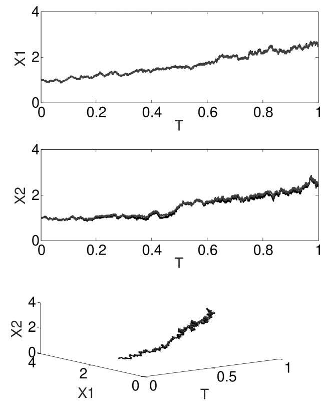
Figure 2: Simulation of the Geometric Brownian Motion on $[0,1]$ ($X_{1}(0)=X_{2}(0)=1,\mu_{1}=\mu_{2}=1,\sigma_{1}=\sigma_{2}=0.5,\rho=0.25$)

Appendix A Proofs of results in Section 3

We start by recalling the following algebraic property of the Lévy areas: for each $0\leq r<s<t$

$$A_{i,j}\left(r,t\right)=A_{i,j}\left(r,s\right)+A_{i,j}\left(s,t\right)+\left(Z_{i}\left(s\right)-Z_{i}\left(r\right)\right)\left(Z_{j}\left(t\right)-Z_{j}\left(s\right)\right).$$ (A.1)

Using this property and a simple use of the Borel-Cantelli lemma we can obtain the proof of Lemma 3.1.

Proof of Lemma 3.1.

We use (A.1) repeatedly. First, note that

$$A_{i,j}\left(t_{k}^{n},t_{k+1}^{n}\right)= A_{i,j}\left(t_{2k}^{n+1},t_{2k+1}^{n+1}\right)+A_{i,j}\left(t_{2k+1}^{n+1},t_{2k+2}^{n+1}\right)$$

$$+\left(Z_{i}\left(t_{2k+1}^{n+1}\right)-Z_{i}\left(t_{2k}^{n+1}\right)\right)\left(Z_{j}\left(t_{2k+2}^{n+1}\right)-Z_{j}\left(t_{2k+1}^{n+1}\right)\right).$$

We continue, this time splitting $A_{i,j}\left(t_{2k}^{n+1},t_{2k+1}^{n+1}\right)$ and $A_{i,j}\left(t_{2k+1}^{n+1},t_{2k+2}^{n+1}\right)$, thereby obtaining

$$A_{i,j}\left(t_{k}^{n},t_{k+1}^{n}\right)$$

$$= \left(Z_{i}\left(t_{2k+1}^{n+1}\right)-Z_{i}\left(t_{2k}^{n+1}\right)\right)\left(Z_{j}\left(t_{2k+2}^{n+1}\right)-Z_{j}\left(t_{2k+1}^{n+1}\right)\right)$$

$$+A_{i,j}\left(t_{2^{2}k}^{n+2},t_{2^{2}k+1}^{n+2}\right)+A_{i,j}\left(t_{2^{2}k+1}^{n+2},t_{2^{2}k+2}^{n+2}\right)$$

$$+\left(Z_{i}\left(t_{2^{2}k+1}^{n+2}\right)-Z_{i}\left(t_{2^{2}k}^{n+2}\right)\right)\left(Z_{j}\left(t_{2^{2}k+2}^{n+2}\right)-Z_{j}\left(t_{2^{2}k+1}^{n+2}\right)\right)$$

$$+A_{i,j}\left(t_{2^{2}k+2}^{n+2},t_{2^{2}k+3}^{n+2}\right)+A_{i,j}\left(t_{2^{2}k+3}^{n+2},t_{2^{2}k+4}^{n+2}\right)$$

$$+\left(Z_{i}\left(t_{2^{2}k+3}^{n+2}\right)-Z_{i}\left(t_{2^{2}k+2}^{n+2}\right)\right)\left(Z_{j}\left(t_{2^{2}k+4}^{n+2}\right)-Z_{j}\left(t_{2^{2}k+3}^{n+2}\right)\right).$$

Suppose by iterating the previous splitting procedure $m$ times, we have

$$A_{i,j}\left(t_{k}^{n},t_{k+1}^{n}\right)$$ (A.2)

$$= \sum_{h=n+1}^{m}\sum_{l=1}^{2^{h-n-1}}\left[Z_{i}\left(t_{2^{h-n}k+2l-1}^{h}\right)-Z_{i}\left(t_{2^{h-n}k+2l-2}^{h}\right)\right]\left[Z_{j}\left(t_{2^{h-n}k+2l}^{h}\right)-Z_{j}\left(t_{2^{h-n}k+2l-1}^{h}\right)\right]$$

$$+\sum_{l=1}^{2^{m-n-1}}A_{i,j}\left(t_{2^{m-n}k+2l-2}^{m},t_{2^{m-n}k+2l-1}^{m}\right)+\sum_{l=1}^{2^{m-n-1}}A_{i,j}\left(t_{2^{m-n}k+2l-1}^{m},t_{2^{m-n}k+2l}^{m}\right).$$

Then for the $(m+1)$-th iteration, we have

$$A_{i,j}\left(t_{k}^{n},t_{k+1}^{n}\right)$$

$$= \sum_{h=n+1}^{m}\sum_{l=1}^{2^{h-n-1}}\left[Z_{i}\left(t_{2^{h-n}k+2l-1}^{h}\right)-Z_{i}\left(t_{2^{h-n}k+2l-2}^{h}\right)\right]\left[Z_{j}\left(t_{2^{h-n}k+2l}^{h}\right)-Z_{j}\left(t_{2^{h-n}k+2l-1}^{h}\right)\right]$$

$$+\sum_{l=1}^{2^{m-n-1}}\{A_{i,j}\left(t_{2(2^{m-n}k+2l-2)}^{m+1},t_{2(2^{m-n}k+2l-2)+1}^{m+1}\right)$$

$$+A_{i,j}\left(t_{2(2^{m-n}k+2l-2)+1}^{m+1},t_{2(2^{m-n}k+2l-2)+2}^{m+1}\right)$$

$$+\left[Z_{i}\left(t_{2(2^{m-n}k+2l-2)+1}^{m+1}\right)-Z_{i}\left(t_{2(2^{m-n}k+2l-2)}^{m+1}\right)\right]$$

$$\times\left[Z_{i}\left(t_{2(2^{m-n}k+2l-2)+2}^{m+1}\right)-Z_{i}\left(t_{2(2^{m-n}k+2l-2)+1}^{m+1}\right)\right]\}$$

$$+\sum_{l=1}^{2^{m-n-1}}\{A_{i,j}\left(t_{2(2^{m-n}k+2l-1)}^{m+1},t_{2(2^{m-n}k+2l-1)+1}^{m+1}\right)$$

$$+A_{i,j}\left(t_{2(2^{m-n}k+2l-1)+1}^{m+1},t_{2(2^{m-n}k+2l-1)+2}^{m+1}\right)$$

$$+\left[Z_{i}\left(t_{2(2^{m-n}k+2l-1)+1}^{m+1}\right)-Z_{i}\left(t_{2(2^{m-n}k+2l-1)}^{m+1}\right)\right]$$

$$\times\left[Z_{i}\left(t_{2(2^{m-n}k+2l-1)+2}^{m+1}\right)-Z_{i}\left(t_{2(2^{m-n}k+2l-1)+1}^{m+1}\right)\right]\}$$

$$= \sum_{h=n+1}^{m+1}\sum_{l=1}^{2^{h-n-1}}\left[Z_{i}\left(t_{2^{h-n}k+2l-1}^{h}\right)-Z_{i}\left(t_{2^{h-n}k+2l-2}^{h}\right)\right]\left[Z_{j}\left(t_{2^{h-n}k+2l}^{h}\right)-Z_{j}\left(t_{2^{h-n}k+2l-1}^{h}\right)\right]$$

$$+\sum_{l=1}^{2^{m-n}}A_{i,j}\left(t_{2^{m+1-n}k+2l-2}^{m+1},t_{2^{m+1-n}k+2l-1}^{m+1}\right)+\sum_{l=1}^{2^{m+1-n-1}}A_{i,j}\left(t_{2^{m+1-n}k+2l-1}^{m+1},t_{2^{m+1-n}k+2l}^{m+1}\right).$$

Thus, (A.2) holds by induction.

We next claim that

$$\sum_{l=1}^{2^{m-n-1}}A_{i,j}\left(t_{2^{m-n}k+2l-2}^{m},t_{2^{m-n}k+2l-1}^{m}\right)+\sum_{l=1}^{2^{m-n-1}}A_{i,j}\left(t_{2^{m-n}k+2l-1}^{m},t_{2^{m-n}k+2l}^{m}\right)\rightarrow 0$$ (A.3)

almost surely as $m\rightarrow\infty$. To see this note that

$$P\left(\left|\sum_{l=1}^{2^{m-n-1}}A_{i,j}\left(t_{2^{h-n}k+2l-2}^{h},t_{2^{h-n}k+2l-1}^{h}\right)\right|>1/m\right)$$

$$\leq m^{2}\sum_{l=1}^{2^{m-n-1}}E\left[A_{i,j}^{2}\left(t_{2^{m-n}k+2l-2}^{m},t_{2^{m-n}k+2l-1}^{m}\right)\right]=m^{2}2^{m-n+1}E\int_{0}^{\Delta_{m}}Z_{i}^{2}\left(s\right)ds$$

$$=m^{2}2^{m-n}\Delta_{m}^{2}=2^{-n}m^{2}\Delta_{m}.$$

Since $\sum_{m=1}^{\infty}m^{2}\Delta_{m}<\infty$, we conclude by Borel-Cantelli’s lemma that, almost surely, for $m$ large enough

$$\left|\sum_{l=1}^{2^{m-n-1}}A_{i,j}\left(t_{2^{h-n}k+2l-2}^{h},t_{2^{h-n}k+2l-1}^{h}\right)\right|<1/m$$

Thus, we have (A.3) holds almost surely and therefore, from (A.2), by sending $m\rightarrow\infty$ we obtain the conclusion of the lemma. ∎

Proof of Lemma 3.2.

Let $N_{i,1}=\max\{n\geq 1:|W_{i,k}^{n}|>4\sqrt{n+1}\mbox{ for some }1\leq k\leq 2^{n-1}\}$. Then $N_{1}=\max_{i}\{N_{i,1}\}$.

$$E[N_{i,1}] = \sum_{n=1}^{\infty}P(N_{i,1}\geq n)$$

$$\leq \sum_{n=1}^{\infty}\sum_{m=n}^{\infty}\sum_{k=1}^{2^{m-1}}P(|W_{i,k}^{m}|>4\sqrt{m+1})$$

$$\leq \sum_{n=1}^{\infty}\sum_{m=n}^{\infty}2^{m-1}\exp(-8m)$$

$$\leq \sum_{n=1}^{\infty}\frac{\exp(-(8-\log 2)n)}{1-\exp(-(8-\log 2))}$$

$$= \frac{\exp(-(8-\log 2))}{(1-\exp(-(8-\log 2)))^{2}}<\infty$$

Thus $E[N]<\infty$. We also notice that $E[N_{1}]$ is independent of our choice of $\alpha$ and $\beta$. ∎

Proof of Lemma 3.3.

For any interval $[t,t+\delta]\subset[0,1]$, there exists $m\in\mathbb{Z}^{+}$, such that $2^{-(m+1)}\leq\delta\leq 2^{-m}$. We next divide the analysis into two cases.

• There exist two level $m$ dyadic points $t_{k}^{m}$ and $t_{k+1}^{m}$, such that $[t,t+\delta]\subset[t_{k}^{m},t_{k+1}^{m}]$.

• There exist three level $m$ dyadic points $t_{k}^{m}$, $t_{k+1}^{m}$ and $t_{k+1}^{m}$, such that $t\in[t_{k}^{m},t_{k+1}^{m}]$ and $t+\delta\in[t_{1}^{m},t_{k+2}^{m}]$.

In Case 1, using the Lévy-Ciesielski construction, we have

$$|Z(t+\delta)-Z(t)|\leq 2^{-m}V^{0}+\sum_{n=1}^{m}2^{-m+\frac{n-1}{2}}V^{n}+\sum_{n=m+1}^{\infty}2^{-\frac{n+1}{2}}V^{n}.$$

Since $\delta\geq 2^{-(m+1)}$, we have

$$\frac{|Z(t+\delta)-Z(t)|}{\delta^{\alpha}}$$

$$\leq 2^{2\alpha}\left(2^{-(1-\alpha)m-\alpha}V^{0}+\sum_{n=1}^{m}2^{-(1-\alpha)m-\alpha+\frac{n-1}{2}}V^{n}+\sum_{n=m+1}^{\infty}2^{-\frac{n+1}{2}+\alpha(m+1)}V^{n}\right)$$

$$\leq 2^{2\alpha}\left(\sum_{n=0}^{m}2^{-(1-\alpha)n+\frac{n}{2}}V^{n}+\sum_{n=m+1}^{\infty}2^{-\frac{n}{2}+\alpha n}V^{n}\right)$$

$$\leq 2^{2\alpha}\sum_{n=0}^{\infty}2^{-n(\frac{1}{2}-\alpha)}V^{n}.$$

Similar to Case 1, in Case 2, we have

$$|Z(t+\delta)-Z(t)| \leq |Z(t_{k+1}^{m})-Z(t)|+|Z(t+\delta)-Z(t_{k+1}^{m})|$$

$$\leq 2\left(V^{0}+\sum_{n=1}^{m}2^{-m+\frac{n-1}{2}}V^{n}+\sum_{n=m+1}^{\infty}2^{-\frac{n+1}{2}}V^{n}\right).$$

Then

$$\frac{|Z(t+\delta)-Z(t)|}{\delta^{\alpha}}\leq 2^{2\alpha+1}\sum_{n=0}^{\infty}2^{-n(\frac{1}{2}-\alpha)}V^{n}.$$

As the interval $[t,t+\delta]$ is arbitrarily chosen, we obtain the result. ∎

Proof of Lemma 3.4.

For $i\neq j$, let $N_{i,j,2}=\max\{n:|L_{i,j}^{n}(m)-L_{i,j}^{n}(l)|>(m-l)^{\beta}\Delta_{n}^{2\alpha}\text{ for some }0\leq l<m\leq 2^{n-1}\}$. Then $N_{2}=\max_{1\leq i,j\leq d^{\prime},i\neq j}\{N_{i,j,2}\}$.

Fix any $(i,j)$ pair, Define

$$\mathcal{C}_{n}=\{|L_{i,j}^{n}(m)-L_{i,j}^{n}(l)|>(m-l)^{\beta}\Delta_{n}^{2\alpha}\text{ for some }0\leq l<m\leq 2^{n-1}\}.$$

We will show that the events $\{\mathcal{C}_{n}:n\geq 0\}$ occur finitely many times. Note that

$$P\left(\mathcal{C}_{n}\right)\leq\sum_{0\leq l<m\leq 2^{n-1}}2P\left(\left(L_{i,j}^{n}(m)-L_{i,j}^{n}(l)\right)>(m-l)^{\beta}\Delta_{n}^{2\alpha}\right).$$ (A.4)

Also observe that for fixed $m$ and $n$, $L_{i,j}^{n}\left(m\right)$ is the sum of $m$ i.i.d. random variables, each of which is distributed as $(Z_{i}(t_{1}^{n})-Z_{i}(t_{0}^{n}))(Z_{j}(t_{2}^{n})-Z_{j}(t_{1}^{n}))$ and

$$E\left[\exp\left(\theta(Z_{i}(t_{1}^{n})-Z_{i}(t_{0}^{n}))(Z_{j}(t_{2}^{n})-Z_{j}(t_{1}^{n}))\right)\right]=\left(1-\theta^{2}\Delta_{n}^{2}\right)^{-1/2}.$$

We apply Chernoff’s bound and have

$$P\left(\left(L_{i,j}^{n}(m)-L_{i,j}^{n}(l)\right)>(m-l)^{\beta}\Delta_{n}^{2\alpha}\right)$$

$$\leq \exp\left(-\theta\left(m-l\right)^{\beta}\Delta_{n}^{2\alpha}-\frac{1}{2}(m-l)\log\left(1-\theta^{2}\Delta_{n}^{2}\right)\right).$$

Select $\theta=\theta^{\prime}\left(m-l\right)^{-1/2}\Delta_{n}^{-1}$ for $\theta^{\prime}\in\left(0,1/4\right)$

$$P\left(\left(L_{i,j}^{n}(m)-L_{i,j}^{n}(l)\right)>(m-l)^{\beta}\Delta_{n}^{2\alpha}\right)\leq\exp\left(-\theta^{\prime}\left(m-l\right)^{\beta-1/2}\Delta_{n}^{2\alpha-1}+1\right).$$

Hence,

$$P\left(\mathcal{C}_{n}\right)\leq\sum_{0\leq l<m\leq 2^{n-1}}2\exp\left(-\theta^{\prime}\left(m-l\right)^{\beta-1/2}\Delta_{n}^{2\alpha-1}+1\right)\leq 2^{2n}\exp\left(-\theta^{\prime}2^{n\left(1-2\alpha\right)}\right).$$ (A.5)

We notice that $2\alpha<1$.

$$E[N_{i,j,2}]=\sum_{n=1}^{\infty}P(N_{i,j,2}\geq n)$$

and

$$P(N_{i,j,2}\geq n)\leq\sum_{m=n}^{\infty}P(C_{m})$$

From (A.5), we denote

$$M:=\min\left\{n:2^{2n}\exp\left(-\theta^{\prime}2^{n\left(1-2\alpha\right)}\right)<1/4\right\}.$$

Then $M=o\left((1-2\alpha)^{-2}\right)$. We also notice that for $n\geq M$,

$$2^{2(n+1)}\exp\left(-\theta^{\prime}2^{(n+1)\left(1-2\alpha\right)}\right)<\left(2^{2n}\exp\left(-\theta^{\prime}2^{n\left(1-2\alpha\right)}\right)\right)^{2}$$

Thus, $\sum_{m=M+k}^{\infty}P(\mathcal{C}_{m})\leq(1/2)^{k}$ and

$$E[N_{i,j,2}]\leq M-1+\sum_{n=M}^{\infty}\sum_{m=n}^{\infty}P(\mathcal{C}_{m})\leq M$$

Thus, $E[N_{2}]=o\left((1-2\alpha)^{-2}\right)$. ∎

The proof of Corollary 3.1 follows directly from Lemma 3.1 and Lemma 3.4.

Proof of Corollary 3.1.

Using Lemma 3.1 we obtain that

$$R_{i,j}^{n}(t_{l}^{n},t_{m}^{n})=\sum_{k=l+1}^{m}\sum_{h=n+1}^{\infty}(L_{i,j}^{h}(2^{h-n}(k+1))-L_{i,j}^{h}(2^{h-n}k)).$$ (A.6)

On the other hand, due to Lemma 3.4 if $n\geq N_{2}$

$$\sum_{k=l+1}^{m}\sum_{h=n+1}^{\infty}|L_{i,j}^{h}(2^{h-n}(k+1))-L_{i,j}^{h}(2^{h-n}k)|$$

$$\leq \sum_{k=l+1}^{m}\sum_{h=n+1}^{\infty}(2^{-n}(k+1)-2^{-n}k)^{\beta}\Delta_{h}^{2\alpha-\beta}<\infty$$

because $\beta<2\alpha$. Thus (by Fubini’s theorem) the order of the summations in (A.6) can be exchanged and we obtain the result. ∎

Proof of Lemma 3.5.

We start by showing the bound on $\Gamma_{R}$. By the definition of $\Gamma_{L}$, for any $n$

$$|L_{i,j}^{n}(m)-L_{i,j}^{n}(l)|\leq\Gamma_{L}(m-l)^{\beta}\Delta_{n}^{2\alpha}.$$

Consequently, for any $0\leq l<m\leq 2^{n-1}$,

$$|R_{i,j}^{n}(t_{l}^{n},t_{m}^{n})| \leq\sum_{h=n+1}^{\infty}\left|L_{i,j}^{h}(2^{h-n}m)-L_{i,j}^{h}(2^{h-n}l)\right|$$

$$\leq\sum_{h=n+1}^{\infty}\Gamma_{L}(m-l)^{\beta}2^{(h-n)\beta}\Delta_{h}^{2\alpha}=\Gamma_{L}(m-l)^{\beta}\Delta_{n}^{\beta}\sum_{h=n+1}^{\infty}\Delta_{h}^{2\alpha-\beta}$$

$$=\Gamma_{L}(t_{m}^{n}-t_{l}^{n})^{\beta}\Delta_{n}^{2\alpha-\beta}\frac{2^{-(2\alpha-\beta)}}{1-2^{-(2\alpha-\beta)}}.$$

Therefore, we conclude that

$$\Gamma_{R} :=\max_{1\leq i,j\leq d^{\prime}}\sup_{n\geq 0}\sup_{0\leq s<t\leq 1,s,t\in D_{n}}\frac{|R_{i,j}^{n}(s,t)|}{|t-s|^{\beta}\Delta_{n}^{2\alpha-\beta}}$$

$$\leq\Gamma_{L}\frac{2^{-(2\alpha-\beta)}}{1-2^{-(2\alpha-\beta)}}.$$

Let $r(n,l,m)=\min\{h:|t_{m}^{n}-t_{l}^{n}|\geq\Delta_{h}\}$. For simplicity of notation, we define the following sequence of operators of time:

$$\underline{s}^{h}(t_{l}^{n})=\min\{t_{k}^{h}:t_{k}^{h}\geq t_{l}^{n}\}$$

$$\bar{s}^{h}(t_{m}^{n})=\max\{t_{k}^{h}:t_{k}^{h}\leq t_{m}^{n}\}$$

for $r(n,l,m)\leq h\leq n$.
Then

$$|A_{i,j}(t_{l}^{n},t_{m}^{n})|$$

$$\leq|A_{i,j}(t_{l}^{n},\underline{s}^{n-1}(t_{l}^{n}))|+|A_{i,j}(\underline{s}^{n-1}(t_{l}^{n}),\bar{s}^{n-1}(t_{m}^{n}))|+|A_{i,j}(\bar{s}^{n-1}(t_{m}^{n}),t_{m}^{n})|$$

$$+|Z_{i}(\underline{s}^{n-1}(t_{l}^{n}))-Z_{i}(t_{l}^{n})||Z_{j}(\bar{s}^{n-1}(t_{m}^{n}))-Z_{j}(\underline{s}^{n-1}(t_{l}^{n}))|$$

$$+|Z_{i}(\bar{s}^{n-1}(t_{m}^{n}))-Z_{i}(t_{l}^{n})||Z_{j}(t_{m}^{n})-Z_{j}(\bar{s}^{n-1}(t_{m}^{n}))|$$

Suppose by iterating the above procedure up to level $\gamma$, where $r(n,l,m)<\gamma<n$, we have

$$|A_{i,j}(t_{l}^{n},t_{m}^{n})|$$

$$\leq \sum_{h=\gamma+1}^{n}|A_{i,j}(\underline{s}^{h}(t_{l}^{n}),\underline{s}^{h-1}(t_{l}^{n}))|+|A_{i,j}(\underline{s}^{\gamma}(t_{l}^{n}),\bar{s}^{\gamma}(t_{m}^{n}))|$$

$$+\sum_{h=\gamma+1}^{n}|A_{i,j}(\bar{s}^{h}(t_{m}^{n}),\bar{s}^{h-1}(t_{m}^{n}))|$$

$$+\sum_{h=\gamma+1}^{n}|Z_{i}(\underline{s}^{h}(t_{l}^{n}))-Z_{i}(\underline{s}^{h-1}(t_{l}^{n}))||Z_{j}(\bar{s}^{h-1}(t_{m}^{n}))-Z_{j}(\underline{s}^{h-1}(t_{l}^{n}))|$$

$$+\sum_{h=\gamma+1}^{n}|Z_{i}(\bar{s}^{h-1}(t_{m}^{n}))-Z_{i}(\underline{s}^{h}(t_{l}^{n}))||Z_{j}(\bar{s}^{h}(t_{m}^{n}))-Z_{j}(\bar{s}^{h-1}(t_{m}^{n}))|$$

Then for level $\gamma-1$, as $\underline{s}^{h-1}(\underline{s}^{h}(t_{l}^{n}))=\underline{s}^{h-1}(t_{l}^{n})$ and $\bar{s}^{h-1}(\bar{s}^{h}(t_{m}^{n}))=\bar{s}^{h-1}(t_{m}^{n})$ for $h<n$, we have

$$|A_{i,j}(t_{l}^{n},t_{m}^{n})|$$

$$\leq \sum_{h=\gamma+1}^{n}|A_{i,j}(\underline{s}^{h}(t_{l}^{n}),\underline{s}^{h-1}(t_{l}^{n}))|$$

$$+|A_{i,j}(\underline{s}^{\gamma}(t_{l}^{n}),\underline{s}^{\gamma-1}(\underline{s}^{\gamma}(t_{l}^{n})))|$$

$$+|A_{i,j}(\underline{s}^{\gamma-1}(\underline{s}^{\gamma}(t_{l}^{n})),\bar{s}^{\gamma-1}(\bar{s}^{\gamma}(t_{m}^{n})))|+|A_{i,j}(\bar{s}^{\gamma-1}(\bar{s}^{\gamma}(t_{m}^{n})),\bar{s}^{\gamma}(t_{m}^{n}))|$$

$$+|Z_{i}(\underline{s}^{\gamma-1}\underline{s}^{\gamma}((t_{l}^{n})))-Z_{i}(\underline{s}^{\gamma}(t_{l}^{n}))||Z_{j}(\bar{s}^{\gamma-1}(\bar{s}^{\gamma}((t_{m}^{n})))-Z_{j}(\underline{s}^{\gamma-1}(\underline{s}^{\gamma}(t_{l}^{n})))|$$

$$+|Z_{i}(\bar{s}^{\gamma-1}(\bar{s}^{\gamma}(t_{m}^{n})))-Z_{i}(\underline{s}^{\gamma}(t_{l}^{n}))||Z_{j}(\bar{s}^{\gamma}(t_{m}^{n}))-Z_{j}(\bar{s}^{\gamma-1}(\bar{s}^{\gamma}(t_{m}^{n})))|$$

$$+\sum_{h=r(n,l,m)+1}^{n}|A_{i,j}(\bar{s}^{h}(t_{m}^{n}),\bar{s}^{h-1}(t_{m}^{n}))|$$

$$= \sum_{h=\gamma}^{n}|A_{i,j}(\underline{s}^{h}(t_{l}^{n}),\underline{s}^{h-1}(t_{l}^{n}))|+|A_{i,j}(\underline{s}^{\gamma-1}(t_{l}^{n}),\bar{s}^{\gamma-1}(t_{m}^{n}))|$$

$$+\sum_{h=\gamma}^{n}|A_{i,j}(\bar{s}^{h}(t_{m}^{n}),\bar{s}^{h-1}(t_{m}^{n}))|$$

$$+\sum_{h=\gamma}^{n}|Z_{i}(\underline{s}^{h-1}(t_{l}^{n}))-Z_{i}(\underline{s}^{h}(t_{l}^{n}))||Z_{j}(\bar{s}^{h-1}(t_{m}^{n}))-Z_{j}(\underline{s}^{h-1}(t_{l}^{n}))|$$

$$+\sum_{h=\gamma}^{n}|Z_{i}(\bar{s}^{h-1}(t_{m}^{n}))-Z_{i}(\underline{s}^{h}(t_{l}^{n}))||Z_{j}(\bar{s}^{h}(t_{m}^{n}))-Z_{j}(\bar{s}^{h-1}(t_{m}^{n}))|$$

Thus, the following inequality holds by induction.

$$|A_{i,j}(t_{l}^{n},t_{m}^{n})|$$

$$\leq \sum_{h=r(n,l,m)+1}^{n}|A_{i,j}(\underline{s}^{h}(t_{l}^{n}),\underline{s}^{h-1}(t_{l}^{n}))|+|A_{i,j}(\underline{s}^{r(n,l,m)}(t_{l}^{n}),\bar{s}^{r(n,l,m)}(t_{m}^{n}))|$$

$$+\sum_{h=r(n,l,m)+1}^{n}|A_{i,j}(\bar{s}^{h}(t_{m}^{n}),\bar{s}^{h-1}(t_{m}^{n}))|$$

$$+\sum_{h=r(n,l,m)+1}^{n}|Z_{i}(\underline{s}^{h-1}(t_{l}^{n}))-Z_{i}(\underline{s}^{h}(t_{l}^{n}))||Z_{j}(\bar{s}^{h-1}(t_{m}^{n}))-Z_{j}(\underline{s}^{h-1}(t_{l}^{n}))|$$

$$+\sum_{h=r(n,l,m)+1}^{n}|Z_{i}(\bar{s}^{h-1}(t_{m}^{n}))-Z_{i}(\underline{s}^{h}(t_{l}^{n}))||Z_{j}(\bar{s}^{h}(t_{m}^{n}))-Z_{j}(\bar{s}^{h-1}(t_{m}^{n}))|$$

We make the following important observations,

$$\underline{s}^{h-1}(t_{l}^{n})-\underline{s}^{h}(t_{l}^{n}) =\begin{cases}0&\text{if }\underline{s}^{h-1}(t_{l}^{n})=\underline{s}^{h}(t_{l}^{n})\\ \Delta_{h}&\text{otherwise}\end{cases}$$

$$\bar{s}^{h}(t_{m}^{n})-\bar{s}^{h-1}(t_{m}^{n}) =\begin{cases}0&\text{if }{s}^{h-1}(t_{m}^{n})=\bar{s}^{h}(t_{m}^{n})\\ \Delta_{h}&\text{otherwise}\end{cases}$$

$$\bar{s}^{r(n,l,m)}(t_{m}^{n})-\underline{s}^{r(n,l,m)}(t_{l}^{n}) =\begin{cases}0&\text{if }\underline{s}^{r(n,l,m)}(t_{l}^{n})=\bar{s}^{r(n,l,m)}(t_{m}^{n})\\ \Delta_{r(n,l,m)}&\text{otherwise.}\end{cases}$$

Then

$$\frac{|A_{i,j}(t_{l}^{n},t_{m}^{n})|}{(t_{m}^{n}-t_{l}^{n})^{2\alpha}}$$

$$\leq \sum_{h=r+1}^{n}\Gamma_{R}\frac{\Delta_{h}^{2\alpha}}{\Delta_{r(n,l,m)}^{2\alpha}}+\Gamma_{R}+\sum_{h=r+1}^{n}\Gamma_{R}\frac{\Delta_{h}^{2\alpha}}{\Delta_{r(n,l,m)}^{2\alpha}}+\sum_{h=r+1}^{n}||Z||_{\alpha}^{2}\frac{\Delta_{h}^{\alpha}}{\Delta_{r(n,l,m)}^{\alpha}}+\sum_{h=r+1}^{n}||Z||_{\alpha}^{2}\frac{\Delta_{h}^{\alpha}}{\Delta_{r}^{\alpha}}$$

$$\leq \Gamma_{R}\frac{2}{1-2^{-2\alpha}}+||Z||_{\alpha}^{2}\frac{2^{1-\alpha}}{1-2^{-\alpha}}.$$

Therefore,

$$||A||_{2\alpha} :=\max_{1\leq i\leq j\leq d^{\prime}}\sup_{n\geq 1}\sup_{0\leq s<t\leq 1;s,t\in D_{n}}\frac{\left|A_{i,j}\left(s\right)\right|}{\left|t-s\right|^{2\alpha}}$$

$$\leq\Gamma_{R}\frac{2}{1-2^{-2\alpha}}+||Z||_{\alpha}^{2}\frac{2^{1-\alpha}}{1-2^{-\alpha}}.$$

∎

Appendix B Proofs of results in Section 5

B.0.1 Proof of results in Section 5.1

Proofs of Lemma 5.1.

We first notice that $t_{2k}^{n}=t_{k}^{n-1}$ for $k=0,1,2,\dots,2^{n-1}$. From the Lévy-Ciesielski Construction, we have

$$Z_{i}(t_{2k-1}^{n})=\frac{1}{2}(Z_{i}(t_{k-1}^{n-1})+Z_{i}(t_{k}^{n-1}))+\Delta_{n+1}^{1/2}W_{i,k}^{n}$$

Then

$$\Lambda_{i}^{n}(t_{2k-1}^{n})=Z_{i}(t_{2k-1}^{n})-Z_{i}(t_{k-1}^{n-1})=\frac{1}{2}(Z_{i}(t_{k-1}^{n-1})-Z_{i}(t_{k}^{n-1}))+\Delta_{n+1}^{1/2}W_{i,k}^{n}$$

and

$$\Lambda_{i}^{n}(t_{2k}^{n})=Z_{i}(t_{k}^{n-1})-Z_{i}(t_{2k-1}^{n})=\frac{1}{2}(Z_{i}(t_{k-1}^{n-1})-Z_{i}(t_{k}^{n-1}))-\Delta_{n+1}^{1/2}W_{i,k}^{n}.$$

∎

Before we prove Corollary 5.1, we first provide the following auxiliary result which summarizes basic computations of moment generating functions of quadratic forms of bivariate Gaussian random variables.

Lemma B.1.

Suppose that $Y$ and $Z$ are i.i.d. $N\left(0,1\right)$ random variables, then for any numbers $a_{1},a_{2},b,c_{1},c_{2}\in R$ define

$$\phi\left(a,b,c\right):=E\exp\left(a_{1}Y+a_{2}Z+bYZ+c_{1}Y^{2}+c_{2}Z^{2}\right),$$

then we have that if $\left|2c_{i}\right|<1$ for $i=1,2$, and$\ \left|b\right|<\left(1-2c_{1}\right)\left(1-2c_{2}\right)$

$$\phi(a,b,c)= \left(1-2c_{1}\right)^{-1/2}\left(1-2c_{2}\right)^{-1/2}\left(1-(b\left(1-2c_{1}\right)^{-1/2}\left(1-2c_{2}\right)^{-1/2})^{2}\right)^{-1/2}$$

$$\times\exp\left(\frac{a_{1}^{2}(1-2c_{1})^{-1}+a_{2}^{2}(1-2c_{2})^{-1}+2a_{1}a_{2}b(1-2c_{1})^{-1}(1-2c_{2})^{-1}}{2(1-b^{2}(1-2c_{1})^{-1}(1-2c_{2})^{-1})}\right)$$

Moreover, if we let

$$P^{\prime}\left(Y\in dy,Z\in dz\right)=P\left(Y\in dy,Z\in dz\right)\frac{\exp\left(a_{1}y+a_{2}z+byz+c_{1}y^{2}+c_{2}z^{2}\right)}{\phi\left(\theta;a,b,c\right)},$$

then under $P^{\prime}\left(\cdot\right)$ we have that $\left(Y,Z\right)$ are distributed bivariate Gaussian with covariance matrix

$$\Sigma\left(a,b,c\right)$$

$$= \frac{1}{1-b^{2}\left(1-2c_{1}\right)^{-1}\left(1-2c_{2}\right)^{-1}}$$

$$\times\left(\begin{array}[]{cc}(1-2c_{1})^{-1}&b\left(1-2c_{1}\right)^{-1}\left(1-2c_{2}\right)^{-1}\\ b\left(1-2c_{1}\right)^{-1}\left(1-2c_{2}\right)^{-1}&(1-2c_{2})^{-1}\end{array}\right),$$

and mean vector

$$\mu\left(a,b,c\right)=\Sigma\left(a,b,c\right)\left(\begin{array}[]{c}a_{1}\\ a_{2}\end{array}\right).$$

Proof.

First it follows easily that $E\exp\left(c_{1}Y^{2}+c_{2}Z^{2}\right)=(1-2c_{1})^{-1/2}(1-2c_{2})^{-1/2}$, and under the probability measure

$$P_{1}\left(Y\in dy.Z\in dz\right)=\frac{\exp\left(c_{1}y^{2}+c_{2}z^{2}\right)}{E\left[\exp\left(c_{1}Y^{2}+c_{2}Z^{2}\right)\right]}P\left(Y\in dy\right)P\left(Z\in dz\right)$$

$Y$ and $Z$ are independent with distributions $N(1,(1-2c_{1})^{-1})$ and $N(1,(1-2c_{2})^{-1})$, respectively. Therefore,

$$\phi\left(a,b,c\right)= (1-2c_{1})^{-1/2}(1-2c_{2})^{-1/2}E_{1}\exp\left(a_{1}Y+a_{2}Z+bYZ\right)$$

$$= (1-2c_{1})^{-1/2}(1-2c_{2})^{-1/2}$$

$$\times E[\exp\{a_{1}Y(1-2c_{1})^{-1/2}+a_{2}Z(1-2c_{2})^{-1/2}$$

$$+b(1-2c_{1})^{-1/2}(1-2c_{2})^{-1/2}YZ\}].$$

Now, given $\left|\theta\right|<1$ define $P_{2}\left(\cdot\right)$ via

$$P_{2}\left(Y\in dy,Z\in dz\right)=\frac{P\left(Y\in dy,Z\in dz\right)\exp\left(\chi yz\right)}{E[\exp\left(\chi YZ\right)]}.$$

Observe that

$$P\left(Y\in dy,Z\in dz\right)\exp\left(\chi yz\right)=\frac{1}{2\pi}\exp\left(-y^{2}/2-z^{2}/2+\chi yz\right)$$

and

$$-y^{2}/2-z^{2}/2+\chi yz=-(y,z)\Sigma^{-1}\binom{y}{z}/2,$$

where

$$\Sigma^{-1}=\left(\begin{array}[c]{cc}1&-\chi\\ -\chi&1\end{array}\right),$$

and thus

$$\Sigma=\frac{1}{1-\chi^{2}}\left(\begin{array}[c]{cc}1&\chi\\ \chi&1\end{array}\right).$$

Therefore, under $P_{2}(\cdot)$, ($Y,Z$) is distributed bivariate normal with mean zero and covariance matrix $\Sigma$, with

$$\chi=b(1-2c_{1})^{-1/2}(1-2c_{2})^{-1/2}$$

and we also must have that if $\left|\chi\right|<1$,

$$E\left[\exp\left(\phi YZ\right)\right]=\left(1-\chi^{2}\right)^{-1/2}=\left(1-(b\left(1-2c_{1}\right)^{-1/2}\left(1-2c_{2}\right)^{-1/2})^{2}\right)^{-1/2}.$$

Consequently, we conclude that

$$\phi\left(a,b,c\right)= \left(1-2c_{1}\right)^{-1/2}\left(1-2c_{2}\right)^{-1/2}\left(1-(b\left(1-2c_{1}\right)^{-1/2}\left(1-2c_{2}\right)^{-1/2})^{2}\right)^{-1/2}$$

$$\times E_{2}\left[\exp(a_{1}Y(1-2c_{1})^{-1/2}+a_{2}Z(1-2c_{2})^{-1/2})\right].$$

The final expression for $\phi\left(a,b,c\right)$ is obtained from the fact that

$$E_{2}\left[\exp(a_{1}Y(1-2c_{1})^{-1/2}+a_{2}Z(1-2c_{2})^{-1/2})\right]$$

$$= \exp\left(Var_{2}(a_{1}Y(1-2c_{1})^{-1/2}+a_{2}Z(1-2c_{2})^{-1/2})/2\right).$$

And $P^{\prime}\left(\cdot\right)$ is equivalent to a standard exponentially tilting to the measure $P_{2}(\cdot)$ using as the natural parameter the vector

$$\left(a_{1}(1-2c_{1})^{-1/2},a_{2}(1-2c_{2})^{-1/2}\right),$$

and thus under $P^{\prime}\left(\cdot\right)$ the covariance matrix is the same as under $P_{2}(\cdot)$ and the mean vector is equal to $\mu\left(a,b,c\right)$. ∎

We now are ready to provide the proof of Corollary 5.1.

Proof of Corollary 5.1.

Let us examine the term of the form
$\Lambda_{i}^{n+m}\left(t_{2r-1}^{n+m}\right)\Lambda_{j}\left(t_{2r}^{n+m}\right)$, for $i\neq j$,

$$\Lambda_{i}^{n+m}\left(t_{2r-1}^{n+m}\right)\Lambda_{j}\left(t_{2r}^{n+m}\right)$$

$$= (\Lambda_{i}^{n+m-1}(t_{r}^{n+m-1})/2+\Delta_{n+m+1}^{1/2}W_{i,r}^{n+m})(\Lambda_{j}^{n+m-1}(t_{r}^{n+m-1})/2-\Delta_{n+m+1}^{1/2}W_{j,r}^{n+m})$$

$$= \Lambda_{i}^{n+m-1}(t_{r}^{n+m-1})\Lambda_{j}^{n+m-1}(t_{r}^{n+m-1})/4-\Delta_{n+m+1}W_{i,r}^{n+m}W_{j,r}^{n+m}$$

$$+\Delta_{n+m+1}^{1/2}W_{i,r}^{n+m}\Lambda_{j}^{n+m-1}(t_{r}^{n+m-1})/2-\Delta_{n+m+1}^{1/2}W_{j,r}^{n+m}\Lambda_{i}^{n+m-1}(t_{r}^{n+m-1})/2.$$

Then, we have that Corollary 5.1 follows immediately from Lemma B.1. ∎

Finally, we provide the proof of Corollary 5.2.

Proof of Corollary 5.2.

Recall that for each $r\in\{1,2,...,2^{n}\}$,

$$\Lambda_{i}^{n}(t_{r}^{n}):=(Z_{i}(t_{r}^{n})-Z_{i}(t_{r-1}^{n})).$$

So

$$\Lambda_{i}^{n}(t_{2r-1}^{n}) =\Lambda_{i}^{n}(t_{r}^{n-1})/2+\Delta_{n+1}^{1/2}W_{i,r}^{n},$$

$$\Lambda_{i}^{n}(t_{2r}^{n}) =\Lambda_{i}^{n}(t_{r}^{n-1})/2-\Delta_{n+1}^{1/2}W_{i,r}^{n}.$$

We perform the first iteration in full detail, the rest are immediate just adjusting the notation. From Corollary 5.1 we obtain that, for $i\neq j$,

$$E_{n+m-1}\exp\left(\theta_{0}[L_{i,j}^{n+m}\left(k^{\prime}\right)-L_{i,j}^{n+m}\left(k\right)]\right)$$

$$= \exp\left(\frac{1}{2}\sum_{r=k+1}^{k^{\prime}}\frac{\theta_{0}^{2}\Delta_{n+m+1}}{4\left(1-\theta_{0}^{2}\Delta_{n+m+1}^{2}\right)}\Lambda_{i}\left(t_{r}^{n+m-1}\right)^{2}+\frac{1}{2}\sum_{r=k+1}^{k^{\prime}}\frac{\theta_{0}^{2}\Delta_{n+m+1}}{4\left(1-\theta_{0}^{2}\Delta_{n+m}^{2}\right)}\Lambda_{j}\left(t_{r}^{n+m-1}\right)^{2}\right)$$

$$\times\exp\left(\sum_{r=k+1}^{k^{\prime}}\frac{\theta_{0}\Delta_{n+m+1}}{4\left(1-\theta_{0}^{2}\Delta_{n+m+1}^{2}\right)}\Lambda_{i}\left(t_{r}^{n+m-1}\right)\Lambda_{j}\left(t_{r}^{n+m-1}\right)\right)\times(1-\theta_{0}^{2}\Delta_{n+m+1}^{2})^{-(k^{\prime}-k)/2}.$$

Using the definitions in (5.5) we have that the exponential component

$$\frac{1}{2}\sum_{r=k+1}^{k^{\prime}}\frac{\theta_{0}^{2}\Delta_{n+m+1}}{4\left(1-\theta_{0}^{2}\Delta_{n+m+1}^{2}\right)}\Lambda_{i}\left(t_{r}^{n+m-1}\right)^{2}+\frac{1}{2}\sum_{r=k+1}^{k^{\prime}}\frac{\theta_{0}^{2}\Delta_{n+m+1}}{4\left(1-\theta_{0}^{2}\Delta_{n+m+1}^{2}\right)}\Lambda_{j}\left(t_{r}^{n+m-1}\right)^{2}$$

$$+\sum_{r=k+1}^{k^{\prime}}\frac{\theta_{0}\Delta_{n+m+1}}{4\left(1-\theta_{0}^{2}\Delta_{n+m+1}^{2}\right)}\Lambda_{i}\left(t_{r}^{n+m-1}\right)\Lambda_{j}\left(t_{r}^{n+m-1}\right)$$

is equal to

$$\sum_{r=1}^{2^{n+m-2}}[\eta_{1}\left(t_{2r-1}^{n+m-1}\right)\Lambda_{i}\left(t_{2r-1}^{n+m-1}\right)^{2}+\eta_{1}\left(t_{2r}^{n+m-1}\right)\Lambda_{i}\left(t_{2r}^{n+m-1}\right)^{2}]$$

$$+\sum_{r=1}^{2^{n+m-2}}[\eta_{1}\left(t_{2r-1}^{n+m-1}\right)\Lambda_{j}\left(t_{2r-1}^{n+m-1}\right)^{2}+\eta_{1}\left(t_{2r}^{n+m-1}\right)\Lambda_{j}\left(t_{2r}^{n+m-1}\right)^{2}]$$

$$+\sum_{r=1}^{2^{n+m-2}}[\theta_{1}\left(t_{2r-1}^{n+m-1}\right)\Lambda_{i}\left(t_{2r-1}^{n+m-1}\right)\Lambda_{j}\left(t_{2r-1}^{n+m-1}\right)$$

$$+\theta_{1}\left(t_{2r}^{n+m-1}\right)\Lambda_{i}\left(t_{2r}^{n+m-1}\right)\Lambda_{j}\left(t_{2r}^{n+m-1}\right)].$$

We next expand each of the terms. To simplify the notation, we write

$$x=W_{i,r}^{n+m-1}\text{ \ and \ }y=W_{j,r}^{n+m-1}.$$

Define $\sqrt{\Delta}=\Delta_{n+m}^{1/2}$, put $u=\Lambda_{i}\left(t_{r}^{n+m-2}\right)$ and $v=\Lambda_{j}\left(t_{r}^{n+m-2}\right)$

$$\Lambda_{i}\left(t_{2r-1}^{n+m-1}\right) =u/2+\sqrt{\Delta}x\text{,\ \ \ \ }\Lambda_{i}\left(t_{2r}^{n+m-1}\right)=u/2-\sqrt{\Delta}x,$$

$$\Lambda_{j}\left(t_{2r}^{n+m-1}\right) =v/2+\sqrt{\Delta}y\text{,\ \ \ \ }\Lambda_{j}\left(t_{2r}^{n+m-1}\right)=v/2-\sqrt{\Delta}y.$$

Now, for brevity let us write $\eta_{o}=\eta_{1}\left(t_{2r-1}^{n+m-1}\right)$ and $\eta_{e}=\eta_{1}\left(t_{2r}^{n+m-1}\right)$ (‘o’ is used for odd, and ‘e’ for even)

$$(\eta_{1}\left(t_{2r-1}^{n+m-1}\right)\Lambda_{i}\left(t_{2r-1}^{n+m-1}\right)^{2}+\eta_{1}\left(t_{2r}^{n+m-1}\right)\Lambda_{i}\left(t_{2r}^{n+m-1}\right)^{2}$$

$$+\eta_{1}\left(t_{2r-1}^{n+m-1}\right)\Lambda_{j}\left(t_{2r-1}^{n+m-1}\right)^{2}+\eta_{1}\left(t_{2r}^{n+m-1}\right)\Lambda_{j}\left(t_{2r}^{n+m-1}\right)^{2})$$

$$= \left(\eta_{o}\left(u/2+\sqrt{\Delta}x\right)^{2}+\eta_{e}\left(u/2-\sqrt{\Delta}x\right)^{2}+\eta_{o}\left(v/2+\sqrt{\Delta}y\right)^{2}+\eta_{e}\left(v/2-\sqrt{\Delta}y\right)^{2}\right)$$

$$= \frac{1}{4}u^{2}(\eta_{e}+\eta_{o})+\frac{1}{4}v^{2}(\eta_{e}+\eta_{o})+u(\eta_{o}-\eta_{e})\sqrt{\Delta}x+v(\eta_{o}-\eta_{e})\sqrt{\Delta}y$$

$$+(\eta_{e}+\Delta\eta_{o})\Delta x^{2}+(\eta_{e}+\eta_{o})\Delta y^{2}.$$

Likewise, put $\theta_{o}=\theta_{1}\left(t_{2r-1}^{n+m-1}\right)$ and $\theta_{e}=\theta_{1}\left(t_{2r}^{n+m-1}\right)$

$$\theta_{1}\left(t_{2r-1}^{n+m-1}\right)\Lambda_{i}\left(t_{2r-1}^{n+m-1}\right)\Lambda_{j}\left(t_{2r-1}^{n+m-1}\right)+\theta_{1}\left(t_{2r}^{n+m-1}\right)\Lambda_{i}\left(t_{2r}^{n+m-1}\right)\Lambda_{j}\left(t_{2r}^{n+m-1}\right)$$

$$= \theta_{o}\left(u/2+\sqrt{\Delta}x\right)\left(v/2+\sqrt{\Delta}y\right)+\theta_{e}\left(u/2-\sqrt{\Delta}x\right)\left(v/2-\sqrt{\Delta}y\right)$$

$$= \frac{1}{4}uv(\theta_{e}+\theta_{o})+(\theta_{e}+\theta_{o})\Delta xy+\frac{1}{2}v(\theta_{o}-\theta_{e})\sqrt{\Delta}x+\frac{1}{2}u(\theta_{o}-\theta_{e})\sqrt{\Delta}y$$

We then collect the terms free of $x$ and $y$ and obtain

$$\frac{u^{2}}{4}\left(\eta_{e}+\eta_{o}\right)+\frac{v^{2}}{4}\left(\eta_{e}+\eta_{o}\right)+\frac{uv}{4}(\theta_{e}+\theta_{o}).$$

Now the coefficients of $x,y,x^{2},y^{2},$ and $xy$

$$\{u(\eta_{o}-\eta_{e})+\frac{1}{2}v(\theta_{o}-\theta_{e})\}\sqrt{\Delta}x+\{v(\eta_{o}-\eta_{e})+\frac{1}{2}u(\theta_{o}-\theta_{e})\}\sqrt{\Delta}y$$

$$+(\eta_{e}+\eta_{o})\Delta x^{2}+(\eta_{e}+\eta_{o})\Delta y^{2}$$

$$+(\theta_{e}+\theta_{o})\Delta xy.$$

And finally we can apply Lemma B.1 to get the corresponding results. ∎

B.0.2 Proofs of results in Section 5.2

Proof of Lemma 5.2.

Recalling expression (5.6), we establish the bound for $E_{n}\left[\exp\left(\theta_{0}\{L_{i,j}^{n+1}(k^{\prime})-L_{i,j}^{n+m}(k)\}\right)\right]$, for $i\neq j$, by controlling the contribution of the term

$${\displaystyle\prod\limits_{l=2}^{m}}{\displaystyle\prod\limits_{r=1}^{2^{n+m-l}}}C\left(t_{r}^{n+m-l}\right).$$ (B.1)

and the exponential term

$$\exp\left(\sum_{r=1}^{2^{n}}\theta_{m}(t_{r}^{n})\Lambda_{i}(t_{r}^{n})\Lambda_{j}(t_{r}^{n})+\sum_{r=1}^{2^{n}}\eta_{m}(t_{r}^{n})\left(\Lambda_{i}(t_{r}^{n})^{2}+\Lambda_{j}(t_{r}^{n})^{2}\right)\right)$$ (B.2)

separately.

We start by analyzing $\theta_{l}$ and $\eta_{l}$. From Corollary 5.1, we have

$$\theta_{1}=\frac{\theta_{0}}{4\left(1-\theta_{0}^{2}\Delta_{n+m+1}^{2}\right)}\mbox{ and }\eta_{1}=\frac{\theta_{0}^{2}\Delta_{n+m+1}}{8\left(1-\theta_{0}^{2}\Delta_{n+m+1}^{2}\right)}.$$

We notice that $2\eta_{1}\leq\theta_{1}^{2}\Delta_{n+m+1}\leq(5/2)\eta_{1}$.

Let

$$u=\max\{h:k^{\prime}-k>2^{h}\}.$$

We also denote

$$\underline{b}(l):=\min\{r:\theta_{l}(t_{r}^{n+m-l})>0\}$$

and

$$\bar{b}(l):=\max\{r:\theta_{l}(t_{r}^{n+m-l})>0\}.$$

The strategy throughout the rest of the proof proceeds as follows. We have that the $\theta_{l}(t_{r}^{n+m-l})$’s and $\eta_{l}(t_{r}^{n+m-l})$’s, $r=1,2,\dots,2^{n+m-l}$, are nonnegative. We also have that for $l\leq u\wedge m$, the number of positive $\theta_{l}(t_{r}^{n+m-l})$’s and $\eta_{l}(t_{r}^{n+m-l})$’s reduces by about a half at each step $l$ and also the actual value of the positive $\theta_{l}(t_{r}^{n+m-l})$’s and $\eta_{l}(t_{r}^{n+m-l})$’s shrinks by at least $1/2$. We will establish that if $m>u$, for $u<l\leq m$, there are at most two positive $\theta_{l}(t_{r}^{n+m-l})$’s and two positive $\eta_{l}(t_{r}^{n+m-l})$’s and at each step $l$, their values shrink by more than $2^{-3/2}$. Using these observations we will establish some facts and then use them to estimate (B.1) and finally (B.2). We now proceed to carry out this strategy.

We first verify the following claims.

Claim 1:

For $l\leq u$, we claim that $\theta_{l}(t_{r}^{n+m-l}),\eta_{l}(t_{r}^{n+m-l})\geq 0$ for all $r=1,2,\dots,2^{n+m-l}$ and $\theta_{l}(t_{r}^{n+m-l})$’s are equal for $r\in(\underline{b}(l),\bar{b}(l))$ and we denote their values as $\theta_{l}$. So, following the recursion in (5.5) we have that $\theta_{l}=\Delta_{l-1}\theta_{1}$. If $\theta_{l}(t_{\underline{b}(l)}^{n+m-l})\neq\theta_{l}(t_{\underline{b}(l)+1}^{n+m-l})$, then $\theta_{l}(t_{\underline{b}(l)}^{n+m-l})<\theta_{l}(t_{\underline{b}(l)+1}^{n+m-l})=\theta_{l}$, and if $\theta_{l}(t_{\bar{b}(l)}^{n+m-l})\neq\theta_{l}(t_{\bar{b}(l)-1}^{n+m-l})$, then $\theta_{l}(t_{\bar{b}(l)}^{n+m-l})<\theta_{l}(t_{\bar{b}(l)-1}^{n+m-l})=\theta_{l}$. Likewise, $\eta_{l}(t_{r}^{n+m-l})$’s are equal for $r\in(\underline{b}(l),\bar{b}(l))$; we denote their common values as $\eta_{l}$ and we have from (5.5) that $\eta_{l}=\Delta_{l-1}\eta_{1}$. If $\eta_{l}(t_{\underline{b}(l)}^{n+m-l})\neq\eta_{l}(t_{\underline{b}(l)+1}^{n+m-l})$, then $\eta_{l}(t_{\underline{b}(l)}^{n+m-l})<\eta_{l}(t_{\underline{b}(l)+1}^{n+m-l})$, and if $\eta_{l}(t_{\bar{b}(l)}^{n+m-l})\neq\eta_{l}(t_{\bar{b}(l)-1}^{n+m-l})$, then $\eta_{l}(t_{\bar{b}}^{n+m-l})<\eta_{l}(t_{\bar{b}(l)-1}^{n+m-l})$. In other words, at each step, $l$ for $l<u$, $\theta_{l}(t_{r}^{n+m-l})$ and $\eta_{l}(t_{r}^{n+m-l})$ decay at rate $1/2$ if it is not at the boundary ($r\in(\underline{b}(l),\bar{b}(l))$), and the boundary ones ($\theta_{l}(t_{\underline{b}(l)}^{n+m-l})$, $\theta_{l}(t_{\bar{b}(l)}^{n+m-l})$ and $\eta_{l}(t_{\underline{b}(l)}^{n+m-l})$, $\eta_{l}(t_{\bar{b}(l)}^{n+m-l})$), may decay at a faster rate.

We now prove the claim by induction using the recursive relation in (5.5). The claim is immediate for $\theta_{1}$ and $\eta_{1}$. Now suppose it holds for $\theta_{l}(t_{r}^{n+m-l})$ and $\eta_{l}(t_{r}^{n+m-l})$, $r=1,2,\dots,2^{n+m-l}$. We next show that the claim holds for $\theta_{l+1}(t_{r}^{n+m-l-1})$, $r=1,2,\dots,2^{n+m-l-1}$, as well. We omit the proof of $\eta_{l+1}(t_{r}^{n+m-l-1})$ here, as it follows exactly the same line of analysis as $\theta_{l+1}(t_{r}^{n+m-l-1})$.

We divide the analysis into five cases.

Case 1. $\theta_{l}\left(t_{2r-1}^{m+n-l}\right)=\theta_{l}\left(t_{2r}^{m+n-l}\right)$ and $\eta_{l}\left(t_{2r-1}^{m+n-l}\right)=\eta_{l}\left(t_{2r}^{m+n-l}\right)$. Then $\theta_{+}^{l+1}\left(t_{r}^{m+n-l}\right)=2\theta_{l}\left(t_{2r-1}^{m+n-l+1}\right)$ and $\theta_{-}^{l+1}\left(t_{r}^{m+n-l}\right)=0$. Likewise $\eta_{+}^{l+1}\left(t_{r}^{m+n-l}\right)=2\eta_{l}\left(t_{2r-1}^{m+n-l+1}\right)$ and $\eta_{-}^{l+1}\left(t_{r}^{m+n-l}\right)=0$. From (5.5), we have $\theta_{l}\left(t_{r}^{m+n-l-1}\right)=\theta_{l-1}\left(t_{2r-1}^{m+n-l+1}\right)/2$ and $\eta_{l}\left(t_{r}^{m+n-l-1}\right)=\eta_{l-1}\left(t_{2r-1}^{m+n-l+1}\right)/2$.

Case 2. $\theta_{l}\left(t_{2r-1}^{m+n-l}\right)=0$, $\theta_{l}\left(t_{2r}^{m+n-l}\right)>0$ and $\eta_{l}\left(t_{2r-1}^{m+n-l}\right)=0$, $\eta_{l}\left(t_{2r}^{m+n-l}\right)>0$. Then we know that $2r=\underline{b}(l)$. We also have $\theta_{+}^{l+1}\left(t_{r}^{m+n-l-1}\right)=\theta_{l}\left(t_{2r}^{m+n-l}\right)$ and $\theta_{-}^{l+1}\left(t_{r}^{m+n-l-1}\right)=-\theta_{l}\left(t_{2r}^{m+n-l}\right)$. Likewise, $\eta_{+}^{l+1}\left(t_{r}^{m+n-l-1}\right)=\eta_{l}\left(t_{2r}^{m+n-l}\right)$ and $\eta_{-}^{l+1}\left(t_{r}^{m+n-l-1}\right)=-\eta_{l}\left(t_{2r}^{m+n-l}\right)$. We rewrite the expression for $\theta_{l+1}(t_{r}^{n+m-l-1})$ in (5.5) as

$$\theta_{l+1}\left(t_{r}^{m+n-l-1}\right)$$

$$= \theta_{+}^{l+1}(t_{r}^{m+n-l-1})\frac{1}{4}+|\theta_{-}^{l+1}(t_{r}^{m+n-l-1})|\times\{h_{l+1}(t_{r}^{m+n-l-1})|\eta_{-}^{l+1}(t_{r}^{m+n-l-1})|$$

$$+\frac{1}{4}h_{l+1}(t_{r}^{m+n-l-1})|\theta_{-}^{l+1}(t_{r}^{m+n-l-1})|\rho_{l+1}(t_{r}^{m+n-l-1})$$

$$+h_{l+1}(t_{r}^{m+n-l-1})\eta_{-}^{l+1}(t_{r}^{m+n-l-1})^{2}\frac{\rho_{l+1}(t_{r}^{m+n-l-1})}{|\theta_{-}^{l+1}(t_{r}^{m+n-l-1})|}\}$$

$$= \theta_{l}(t_{2r}^{m+n-l})\times\{\frac{1}{4}+h_{l+1}(t_{r}^{m+n-l-1})\eta_{l}(t_{2r}^{m+n-l})$$

$$+\frac{1}{4}h_{l+1}(t_{r}^{m+n-l-1})\theta_{l}(t_{2r}^{m+n-l})\rho_{l+1}(t_{r}^{m+n-l-1})$$

$$+h_{l+1}(t_{r}^{m+n-l-1})\eta_{l}(t_{2r}^{m+n-l})^{2}\frac{\rho_{l+1}(t_{r}^{m+n-l-1})}{\theta_{l}(t_{2r}^{m+n-l})}\}$$ (B.3)

As

$$\theta_{l}\Delta_{n+m-l}\leq\theta_{1}\Delta_{n+m-1}\leq\frac{1}{4}$$

and

$$\eta_{l}\Delta_{n+m-l}\leq\eta_{1}\Delta_{n+m-1}\leq\frac{1}{48},$$

then

$$\rho_{l+1}(t_{r}^{m+n-l-1})\leq\frac{\frac{1}{4}\frac{1}{4}}{1-\frac{1}{2}\frac{1}{48}}<\frac{1}{15}$$

and

$$h_{l+1}(t_{r}^{m+n-l-1})\theta_{l}(t_{2r}^{m+n-l})\leq\frac{\frac{1}{4}}{\left(1-\frac{1}{2}\frac{1}{48}\right)\left(1-\frac{1}{15^{2}}\right)}<\frac{1}{3}$$

Likewise,

$$h_{l+1}(t_{r}^{m+n-l-1})\eta_{l}(t_{2r}^{m+n-l})<1/95$$

and

$$\eta_{l}(t_{2r}^{m+n-l})\frac{\rho_{l+1}(t_{r}^{m+n-l-1})}{\theta_{l}(t_{2r}^{m+n-l})}<1/95$$

Plug these in (B.3), we have

$$\frac{1}{4}\theta_{l}\left(t_{2r}^{m+n-l}\right)<\theta_{l+1}\left(t_{r}^{m+n-l-1}\right)<\frac{3}{10}\theta_{l}\leq\frac{3}{5}\theta_{l+1}.$$

Case 3. $\theta_{l}\left(t_{2r-1}^{m+n-l}\right)>0$, $\theta_{l}\left(t_{2r}^{m+n-l}\right)=0$ and $\eta_{l}\left(t_{2r-1}^{m+n-l}\right)>0$, $\eta_{l}\left(t_{2r}^{m+n-l}\right)=0$. Then we know that $2r-1=\bar{b}(l)$. Following the same line of analysis as in Case 2, we have

$$\frac{1}{4}\theta_{l}\left(t_{2r}^{m+n-l}\right)<\theta_{l+1}\left(t_{r}^{m+n-l-1}\right)<\frac{3}{10}\theta_{l}\leq\frac{3}{5}\theta_{l+1}.$$

Case 4. $0<\theta_{l}\left(t_{2r-1}^{m+n-l}\right)<\theta_{l}\left(t_{2r}^{m+n-l}\right)$ and $0<\eta_{l}\left(t_{2r-1}^{m+n-l}\right)<\theta_{l}\left(t_{2r}^{m+n-l}\right)$. Then we know that $2r-1=\underline{b}(l)$. There exist $\xi<1$, such that $\theta_{l}\left(t_{2r-1}^{m+n-l}\right)\leq\xi\theta_{l}\left(t_{2r}^{m+n-l}\right)=\xi\Delta_{l-1}\theta_{1}$ and $\eta_{l}\left(t_{2r-1}^{m+n-l}\right)\leq\xi\eta_{l}\left(t_{2r}^{m+n-l}\right)=\xi\Delta_{l-1}\eta_{1}$. From (5.5), we have

$$\theta_{l+1}\left(t_{r}^{m+n-l-1}\right)$$

$$\leq \theta_{+}^{l+1}(t_{r}^{m+n-l-1})\left\{\frac{1}{4}+h_{l+1}(t_{r}^{m+n-l-1})\eta_{-}^{l+1}(t_{r}^{m+n-l-1})^{2}\frac{\rho_{l+1}(t_{r}^{m+n-l-1})}{\theta_{+}^{l+1}(t_{r}^{m+n-l-1})}\right\}$$

$$+|\theta_{-}^{l+1}(t_{r}^{m+n-l-1})|\times\{h_{l+1}(t_{r}^{m+n-l-1})|\eta_{-}^{l+1}(t_{r}^{m+n-l-1})|$$

$$+\frac{1}{4}h_{l+1}(t_{r}^{m+n-l-1})|\theta_{-}^{l+1}(t_{r}^{m+n-l-1})|\rho_{l+1}(t_{r}^{m+n-l-1})\}.$$

As $|\theta_{-}^{l+1}(t_{r}^{m+n-l-1})|\leq\theta_{l}$ and $|\eta_{-}^{l+1}(t_{r}^{m+n-l-1})|\leq\eta_{l}$, following the same calculation as in Case 2, it is easy to check that

$$\theta_{l+1}\left(t_{r}^{m+n-l-1}\right)<\theta_{+}^{l+1}(t_{r}^{m+n-l-1})\left(\frac{1}{4}+0.01\right)+|\theta_{-}^{l+1}(t_{r}^{m+n-l-1})|\times 0.05.$$

Since $\theta_{l+1}\left(t_{r}^{m+n-l-1}\right)+|\theta_{-}^{l+1}(t_{r}^{m+n-l-1})|=\theta_{l}$, we have

$$\theta_{l+1}\left(t_{r}^{m+n-l-1}\right) <\theta_{l}\left(\left(\frac{1}{4}+0.01-0.05\right)(1+\xi)+0.05\right)$$

$$=\frac{1}{2}\theta_{l}\left(\frac{1}{2}+0.02+0.42\xi\right)<\frac{\theta_{l}}{2}=\theta_{l+1}.$$

Case 5. $\theta_{l}\left(t_{2r-1}^{m+n-l}\right)>\theta_{l}\left(t_{2r}^{m+n-l}\right)>0$ and $\eta_{l}\left(t_{2r-1}^{m+n-l}\right)>\theta_{l}\left(t_{2r}^{m+n-l}\right)>0$. Then we know that $2r=\bar{b}(l)$. Following the same line of analysis as in Case 4, we have

$$\theta_{l+1}\left(t_{r}^{m+n-l-1}\right)<\theta_{l+1}.$$

We thus prove that the claim holds for $\theta_{l+1}(t_{r}^{m+n-l-1})$, $r=1,2,\dots,2^{n+m-l-1}$, as well.

We have established Claim 1. We now continue with a second claim.

Claim 2:

For $u<l<m$, we have at most two positive $\theta_{l}(t_{r}^{m+n-l})$’s, namely $\theta_{l}(t_{\underline{b}(l)}^{m+n-l})$ and $\theta_{l}(t_{\bar{b}(l)}^{m+n-l})$. Notice that it is possible that $\underline{b}(l)=\bar{b}(l)$. We then claim that if $\underline{b}\neq\bar{b}$,$\theta_{l}(t_{\underline{b}(l)}^{m+n-l})\leq\Delta_{l-1}\theta_{1}2^{-(l-u-1)/2}$ and $\theta_{l}(t_{\bar{b}(l)}^{m+n-l})\leq\Delta_{l-1}\theta_{1}2^{-(l-u-1)/2}$. Similarly $\eta_{l}(t_{\underline{b}(l)}^{m+n-l})\leq\Delta_{l-1}\eta_{1}2^{-(l-u-1)/2}$ and $\eta_{l}(t_{\bar{b}(l)}^{m+n-l})\leq\Delta_{l-1}\eta_{1}2^{-(l-u-1)/2}$. If $\underline{b}(l)=\bar{b}(l)$, $\theta_{l}(t_{\underline{b}(l)}^{m+n-l})\leq\Delta_{l-1}\theta_{1}2^{-(l-u-2)/2}$, $\theta_{l}(t_{\bar{b}(l)}^{m+n-l})\leq\Delta_{l-1}\theta_{1}2^{-(l-u-2)/2}$ and $\eta_{l}(t_{\underline{b}(l)}^{m+n-l})\leq\Delta_{l-1}\eta_{1}2^{-(l-u-2)/2}$, $\eta_{l}(t_{\bar{b}(l)}^{m+n-l})\leq\Delta_{l-1}\eta_{1}2^{-(l-u-2)/2}$.

We prove the claim by induction. We shall give the proof of $\theta_{l}(t_{r}^{m+n-l})$ only, as the proof of $\eta_{l}(t_{r}^{m+n-l})$ follows exactly the same line of analysis. For $l=u$, we have the following cases.

i) $\bar{b}(l)=\underline{b}(l)+2$, $\underline{b}(l)$ is odd. In this case, $\theta_{l+1}(t_{(\underline{b}(l)+1)/2}^{m+n-l-1})<\Delta_{l}\theta_{1}$, which follows from the analysis in Case 4 for $l\leq u$. And $\theta_{l+1}(t_{(\bar{b}(l)+1)/2}^{m+n-l-1})<(3/5)\Delta_{l}\theta_{1}$, following the analysis in Case 3 for $l\leq u$.

ii) $\bar{b}(l)=\underline{b}(l)+2$, $\underline{b}(l)$ is even. In this case, $\theta_{l+1}(t_{\underline{b}(l)/2}^{m+n-l-1})<(3/5)\Delta_{l}\theta_{1}$, which follows from the analysis in Case 2 for $l\leq u$. And $\theta_{l+1}(t_{\bar{b}(l)/2}^{m+n-l-1})<\Delta_{l}\theta_{1}$, following the analysis in Case 5, for $l\leq u$.

iii) $\bar{b}(l)=\underline{b}(l)+1$, $\underline{b}(l)$ is odd. In this case, let $\bar{\theta}_{l}=\max\{\theta_{l}(t_{\underline{b}(l)}^{m+n-l}),\theta_{l}(t_{\bar{b}(l)}^{m+n-l})\}$, Then following the same analysis as in Case 4 or Case 5 for $l\leq u$ (depending on which one of $\theta_{l}(t_{\underline{b}(l)}^{m+n-l})$ and $\theta_{l}(t_{\bar{b}(l)}^{m+n-l})$ is smaller), we have $\theta_{l+1}(t_{\bar{b}(l)/2}^{m+n-l-1})<\bar{\theta}_{l}/2\leq\Delta_{l}\theta_{1}$.

iv) $\bar{b}(l)=\underline{b}(l)+1$, $\underline{b}(l)$ is even. In this case, $\theta_{l+1}(t_{\underline{b}(l)/2}^{m+n-l-1})<(3/5)\Delta_{l}\theta_{1}$, which follows from the analysis in Case 2 for $l\leq u$. And $\theta_{l+1}(t_{(\bar{b}(l)+1)/2}^{m+n-l-1})<(3/5)\Delta_{l}\theta_{1}$, following the analysis in Case 3 for $l\leq u$.

Therefore, the claim holds for $u+1$. Suppose the claim holds for $l\geq u+1$. Then when moving from level $l$ to level $l+1$, one of the following three cases can happen.

a) $\bar{b}(l)=\underline{b}(l)+1$ and $\underline{b}(l)$ is even. In this case, following the analysis in Case 2 and Case 3 for $l\leq u$, we have

$$\theta_{l+1}(t_{\underline{b}(l)/2}^{m+n-l-1})\leq\frac{3}{10}\theta_{l}(t_{\underline{b}(l)}^{m+n-l})\leq\Delta_{l}\theta_{1}2^{-(l-u)/2}$$

and

$$\theta_{l+1}(t_{(\bar{b}(l)+1)/2}^{m+n-l-1})\leq\frac{3}{10}\theta_{l}(t_{\bar{b}(l)}^{m+n-l})\leq\Delta_{l}\theta_{1}2^{-(l-u)/2}.$$

b) $\bar{b}(l)=\underline{b}(l)$. In this case, following the analysis in Case 2 or Case 3 for $l\leq u$ (depending on whether $\underline{b}(l)$ is odd or even), we have

$$\theta_{l+1}(t_{\lceil\underline{b}(l)/2\rceil}^{m+n-l-1})\leq\frac{3}{10}\theta_{l}(t_{\underline{b}(l)}^{m+n-l})\leq\Delta_{l}\theta_{1}2^{-(l-u-1)/2}.$$

c) $\bar{b}(l)=\underline{b}(l)+1$ and $\underline{b}(l)$ is odd. In this case, we let $\bar{\theta}_{l}=\max\{\theta_{l}(t_{\underline{b}(l)}^{m+n-l}),\theta_{l}(t_{\bar{b}(l)}^{m+n-l})\}$, Then we can use the same analysis as in Case 4 or Case 5 for $l\leq u$ (depending on which one of $\theta_{l}(t_{\underline{b}(l)}^{m+n-l})$ and $\theta_{l}(t_{\bar{b}(l)}^{m+n-l})$ is smaller) to conclude that

$$\theta_{l+1}(t_{\bar{b}(l)/2}^{m+n-l-1})<\frac{1}{2}\bar{\theta}_{l}\leq\Delta_{l}\theta_{1}2^{-(l-u-1)/2}.$$

We notice that case c) can happen only once.

We are now ready to control the contribution of the term (B.1). As $\Delta_{n+m-l+2}\eta_{+}^{l}(t_{r}^{n+m-l})\leq 1/30$ and $\rho_{l}(t_{r}^{n+m-l})<1/7$, we have when $m\leq u$

$$\prod_{l=2}^{m}\prod_{r=1}^{2^{n+m-l}}C(t_{r}^{n+m-l})$$

$$\leq \prod_{l=2}^{m}\prod_{r=1}^{2^{n+m-l}}\exp\left(4\Delta_{n+m-l+2}\eta_{+}^{l}(t_{r}^{n+m-l})+\rho_{l}(t_{r}^{n+m-l})^{2}\right)$$

$$\leq \prod_{l=2}^{m}\exp\left(\left(16\Delta_{n+m}\eta_{1}+\frac{(4\Delta_{n+m}\theta_{1})^{2}}{(1-8\Delta_{n+m}\eta_{1})^{2}}\right)((k^{\prime}-k)\Delta_{l}+2)\right)$$

$$\leq \prod_{l=2}^{m}\exp\left(\left(\frac{11}{5}\frac{\gamma^{2}}{k^{\prime}-k}\Delta_{n}^{1-2\alpha^{\prime}}+\frac{6}{5}\frac{\gamma^{2}}{k^{\prime}-k}\Delta_{n}^{2-4\alpha^{\prime}}\right)((k^{\prime}-k)\Delta_{l}+2)\right).$$

The last inequality follows from Corollary 2 that $\theta_{1}=\theta_{0}/4(1-\theta_{0}^{2}\Delta_{n+m}^{2})$, $\eta_{1}=\theta_{0}^{2}\Delta_{n+m}/2(1-\theta_{0}^{2}\Delta_{n+m}^{2})$, and our choice of $\theta_{0}=\gamma/(k^{\prime 1/2}\Delta_{n}^{2\alpha^{\prime}}\Delta_{m})$. Then, as $(k^{\prime}-k)^{-1}\leq 2^{-m}$,

$$\prod_{l=2}^{m}\prod_{r=1}^{2^{n+m-l}}C(t_{r}^{n+m-l})$$

$$\leq \exp\left(\frac{11}{5}\gamma^{2}\left(\sum_{l=2}^{m}\Delta_{l}+2(m-1)\Delta_{m}\right)+\frac{6}{5}\gamma^{2}\left(\sum_{l=2}^{u}\Delta_{l}+2(m-1)\Delta_{m}\right)\right)$$

$$\leq \exp\left(\frac{8}{25}\right).$$

When $m>u$,

$$\prod_{l=2}^{m}\prod_{r=1}^{2^{n+m-l}}C(t_{r}^{n+m-l})$$

$$\leq \prod_{l=2}^{m}\prod_{r=1}^{2^{n+m-l}}\exp\left(4\Delta_{n+m-l+2}\eta_{+}^{l}(t_{r}^{n+m-l})+\rho_{l}(t_{r}^{n+m-l})^{2}\right)$$

$$\leq \prod_{l=2}^{u}\exp\left(\left(\frac{11}{5}\frac{\gamma^{2}}{k^{\prime}-k}\Delta_{n}^{1-2\alpha^{\prime}}+\frac{6}{5}\frac{\gamma^{2}}{k^{\prime}-k}\Delta_{n}^{2-4\alpha^{\prime}}\right)((k^{\prime}-k)\Delta_{l}+2)\right)$$

$$\times\prod_{l=u+1}^{m}\exp\left(\frac{11}{5}\frac{\gamma^{2}}{k^{\prime}-k}\Delta_{n}^{1-2\alpha^{\prime}}\Delta_{l-u-2}^{1/2}+\frac{6}{5}\frac{\gamma^{2}}{k^{\prime}-k}\Delta_{n}^{2-4\alpha^{\prime}}\Delta_{l-u-2}\right).$$

As $(k^{\prime}-k)^{-1}\leq 2^{-u}$,

$$\prod_{l=2}^{m}\prod_{r=1}^{2^{n+m-l}}C(t_{r}^{n+m-l})$$

$$\leq \exp\{\frac{11}{5}\gamma^{2}\left(\sum_{l=2}^{u}\Delta_{l}+2(u-1)\Delta_{u}+\sum_{l=u+1}^{m}\Delta_{l-2}^{1/2}\right)$$

$$+\frac{6}{5}\gamma^{2}\left(\sum_{l=2}^{u}\Delta_{l}+2(u-1)\Delta_{u}+\sum_{l=u+1}^{m}\Delta_{l-2}\right)\}$$

$$\leq \exp\left(\frac{1}{2}\right).$$

For (B.2), we notice that under condition (5.8) and (5.9), we have

$$\left|\sum_{r=1}^{2^{n}}\theta_{m}(t_{r}^{n})\Lambda_{i}(t_{r}^{n})\Lambda_{j}(t_{r}^{n})\right| \leq\theta_{1}\Delta_{m-1}\varepsilon_{0}((k^{\prime}-k)\Delta_{m})^{\beta}\Delta_{n}^{2\alpha^{\prime}}+2\theta_{1}\Delta_{m-1}\Delta_{n}^{2\alpha^{\prime}}$$

$$\leq\varepsilon_{0}\gamma(k^{\prime}-k)^{\beta-1/2}+2\gamma,$$

and

$$\left|\sum_{r=1}^{2^{n}}\eta_{m}(t_{r}^{n})\left(\Lambda_{i}(t_{r}^{n})^{2}+\Lambda_{j}(t_{r}^{n})^{2}\right)\right| \leq\left((k^{\prime}-k)\Delta_{m}+2\right)\eta_{1}\Delta_{m-1}2\Delta_{n}^{2\alpha^{\prime}}$$

$$\leq 2\gamma^{2}.$$

Combining the analysis for (B.1) and (B.2), we have

$$E_{n}\exp(\theta_{0}\{L_{i,j}^{n+m}(k^{\prime})-L_{i,j}^{n+m}(k)\})$$

$$\leq \exp\left(\theta_{0}^{2}\Delta_{n+m}^{2}(k^{\prime}-k)+\frac{1}{2}+\varepsilon_{0}\gamma(k^{\prime}-k)^{\beta-1/2}+2\gamma+2\gamma^{2}\right)$$

$$\leq 4\exp\left(\varepsilon_{0}\gamma(k^{\prime}-k)^{\beta-1/2}\right).$$

∎

References

- Bayer et al. [2013] C. Bayer, P. Friz, S. Riedel, and J. Schoenmakers. From rough path estimates to multilevel Monte Carlo. http://arxiv.org/pdf/1305.5779v1.pdf, 2013.
- Beskos and Roberts [2005] A. Beskos and G. Roberts. Exact simulation of diffusions. Annals of Applied Probability, 15:2422–2444, 2005.
- Beskos et al. [2006] A. Beskos, O. Papaspiliopoulos, and G. Roberts. Retrospective exact simulation of diffusion sample paths with applications. Bernoulli, 12(6):1077–1098, 2006. ISSN 1350-7265. 10.3150/bj/1165269151. URL http://dx.doi.org/10.3150/bj/1165269151.
- Beskos et al. [2012] A. Beskos, S. Peluchetti, and G. Roberts. -strong simulation of the Brownian path. Bernoulli, 18(4):1223–1248, 2012. ISSN 1350-7265. 10.3150/11-BEJ383. URL http://dx.doi.org/10.3150/11-BEJ383.
- Blanchet and Chen [2013] J. Blanchet and X. Chen. Steady-state simulation for reflected Brownian motion and related networks. http://arxiv.org/pdf/1202.2062.pdf, 2013.
- Chen and Huang [2013] N. Chen and Z. Huang. Localization and exact simulation of brownian motion-driven stochastic differential equations. Mathematics of Operations Research, 38:591–616, 2013.
- Davie [2007] A.M. Davie. Differential equations driven by rough paths: An approach via discrete approximation. http://arxiv.org/abs/0710.0772, 2007.
- Fritz and Victoir [2010] P. Fritz and N. Victoir. Multidimensional Stochastic Processes as Rough Paths: Theory and Applications, volume 120. Cambridge University Press, 2010.
- Gaines and Lyons [1994] J.G. Gaines and T.J. Lyons. Random generation of stochastic area integrals. SIMA J. Appl. Math, 54(4):1132–1146, 1994.
- Lyons [1998] T.J. Lyons. Differential equations driven by rough signals. Rev. Mat. Iberoamericana, 14(2):215–310, 1998.
- Pollock et al. [2014] M. Pollock, A. Johansen, and G. Roberts. On the exact and -strong simulation of (jump) diffusions. http://arxiv.org/pdf/1302.6964v2.pdf, 2014.
- Rhee and Glynn [2012] C. Rhee and P. Glynn. A new approach to unbiased estimation of sdes. http://arxiv.org/pdf/1207.2452.pdf, 2012.
- Steele [2001] J.M. Steele. Stochastic Calculus and Financial Application. Springer-Verlag, 2001.