Partitioning strategies for the interaction of a fluid with a poroelastic material based on a Nitsche’s coupling approach

M. Bukač martinab@pitt.edu I. Yotov yotov@math.pitt.edu R. Zakerzadeh raz25@pitt.edu P. Zunino paz13@pitt.edu Department of Mathematics, University of Pittsburgh, Pittsburgh, PA 15260, USA Department of Mechanical Engineering & Materials Science, University of Pittsburgh, Pittsburgh, PA 15261, USA
Abstract

We develop a computational model to study the interaction of a fluid with a poroelastic material. The coupling of Stokes and Biot equations represents a prototype problem for these phenomena, which feature multiple facets. On one hand, it shares common traits with fluid-structure interaction. On the other hand it resembles the Stokes-Darcy coupling. For these reasons, the numerical simulation of the Stokes-Biot coupled system is a challenging task. The need of large memory storage and the difficulty to characterize appropriate solvers and related preconditioners for the equations at hand are typical shortcomings of classical discretization methods applied to this problem, such as the finite element method for spatial discretization and finite differences for time stepping. The application of loosely coupled time advancing schemes mitigates these issues, because it allows to solve each equation of the system independently with respect to the others, at each time step. In this work, we develop and thoroughly analyze a loosely coupled scheme for Stokes-Biot equations. The scheme is based on Nitsche’s method for enforcing interface conditions. Once the interface operators corresponding to the interface conditions have been defined, time lagging allows us to build up a loosely coupled scheme with good stability properties. The stability of the scheme is guaranteed provided that appropriate stabilization operators are introduced into the variational formulation of each subproblem. The error of the resulting method is also analyzed, showing that splitting the equations pollutes the optimal approximation properties of the underlying discretization schemes. In order to restore good approximation properties, while maintaining the computational efficiency of the loosely coupled approach, we consider the application of the loosely coupled scheme as a preconditioner for the monolithic approach. Both theoretical insight and numerical results confirm that this is a promising way to develop efficient solvers for the problem at hand.

keywords:
Fluid-structure interaction , poroelasticity , operator-splitting scheme , Nitsche’s method , preconditioning

1 Introduction

Several phenomena in nature involve the interaction of a free fluid with a porous and deformable material. In geomechanics, the behavior of aquifers and groundwater flow is significantly influenced by the interaction of deformation and flow at the pore scale. In the same context, the efficient extraction of oil and gas from the subsurface relies on the ability to predict and control these phenomena. Another example from biology is the perfusion of living tissues, where the fluid carried by the main vessels is distributed by filtration to the surrounding material. All these phenomena are characterized by some common traits. In particular, they share a multiphysics nature, because they are governed by the interaction of fluid and solid mechanics.

In the general framework of continuum mechanics, several models are available to describe these phenomena. To model the free fluid, we consider for simplicity the Stokes equations, under the assumptions of incompressible and Newtonian rheology. A well accepted model for characterizing the behavior of a poroelastic material is provided by the Biot equations. The Biot system consists of the governing equations for the deformation of an elastic skeleton, which is completely saturated with fluid. The average velocity of the fluid in the pores is modelled using the Darcy equation, complemented with an additional term that depends on the volumetric deformation of the porous matrix. Indeed, this term accounts for the poroelastic coupling. In this work we focus on the coupling of the Stokes and Biot models, for phenomena where time and space dependence of the unknowns play a significant role.

The numerical discretization of the problem at hand features several difficulties. With fluid-structure interaction (FSI), it shares the difficulties of combining the Eulerian description of the moving fluid domain with the typical Lagrangian parametrization of the structure. The two reference frames can be merged using the arbitrary Lagrangiann-Eulerian approach [17, 26]. Furthermore, loosely coupled schemes for FSI may turn out to be unconditionally unstable, under a particular range of the physical parameters of the model [10, 20]. This is the so called added-mass effect. On the other hand, accounting for a poroelastic material model requires addressing issues typical of partitioned methods for flows [12, 13, 14] arising in particular for the coupling of Stokes-Darcy models, which represents the paradigm for studying the interaction of free flows with subsurface filtration [8, 9, 11, 15, 16, 29, 28, 38].

These observations suggest that the solution of the time dependent Biot-Stokes coupled equations is challenging from both the theoretical and computational standpoints. Concerning the analysis, the coupled problem and in particular the formulation of appropriate interface conditions has been studied in [5, 33, 39]. From the computational viewpoint, the multiple facets of the problem have been addressed in several studies. For example, the coupling of subsurface flow and geomechanics have been recently addressed in [27, 34, 40]. Depending on the field of application, different formulations are available to couple a free flow with a saturated poroelastic material. In the context of geosciences, this coupled problem is used to model the interaction of the material with fractures, as in [22, 23, 21, 30, 32, 33]. In the context of biomedical applications, FSI problems involving poroelastic materials have not been widely studied. Our work in this direction has been significantly inspired by the seminal study reported in [1, 36].

The objective of this work is to develop and analyze a loosely coupled numerical solver for the coupled Biot-Stokes system. More precisely, we design a time advancing scheme which allows us to independently solve the governing equations of the system at each time step. Resorting to time splitting approaches mitigates the difficulty to identify appropriate solvers for the coupled system and reduces the need of large memory storage. The main drawback of loosely coupled splitting schemes is possible lack of stability and accuracy. To overcome these natural limitations, we adopt a non-standard approach for the approximation of the coupling conditions, which is inspired by Nitsche’s method for the enforcement of boundary conditions, and it consists of adding appropriate interface operators to the variational formulation of the problem. Using time-lagging, the variational coupled problem can be split into three independent subproblems involving the elasticity equation, Darcy equation for flow in porous media and the Stokes problem, respectively. The stability analysis of the resulting scheme shows how to design appropriate stabilization terms that guarantee the stability of the time advancing algorithm. The Nitsche’s coupling approach allows for treating the mixed form of Darcy flow and thus provides accurate approximation to the filtration velocity. This is an alternative to the Lie-splitting scheme developed in [4], which is suitable for the pressure formulation of Darcy flow.

A Nitsche’s coupling has been proposed in [6, 7] for the interaction of a fluid with an elastic structure. Here, we extend those ideas to the case where a porous media flow is coupled to the fluid and the structure. Not only the coupling conditions between the fluid and the porous matrix subregions become significantly more complicated, but also the stability and error analysis involve the characteristic difficulties of both the FSI and Stokes-Darcy decomposition methods. The main drawback of the scheme originally proposed in [6] is accuracy. In [7] the same authors address several modifications of the scheme, mainly based on iterative corrections, to restore the optimal approximation properties that are lost when the equations of the system are split. The splitting scheme proposed in this work also affects the approximation properties of the underlying discretization methods. However, we mitigate this drawback with a different approach than in [7]. Here, we develop a numerical solver where the loosely coupled scheme is acting as a preconditioner for the monolithic problem formulation. In this way, we combine the computational efficiency of the loosely coupled scheme with the accuracy of the discrete coupled problem. Our numerical experiments show that the number of iterations needed to solve the preconditioned problem is almost independent of the spatial and temporal discretization parameters.

The manuscript is organized as follows. In Section 2 we present the governing equations of the prototype problem at hand, complemented by initial, boundary and interface conditions. The numerical discretization scheme, and in particular the approximation of the interface conditions is discussed in Section 3. A thorough analysis of the stability properties of the fully coupled discrete scheme is also presented. Section 4 is devoted to the development and analysis of the loosely coupled scheme. At the end of this section, we exploit the stability analysis of the method to provide insight on the properties of the loosely coupled scheme as a preconditioner for the monolithic scheme. Extensive numerical experiments are discussed in Section 5. The corresponding results support and complement the available theory.

2 Description of the problem

We consider the flow of an incompressible, viscous fluid in a channel bounded by a poroelastic medium. In particular, we are interested in simulating flow through the deformable channel with a two-way coupling between the fluid and the poroleastic structure. The model we consider is similar to the one studied in [4]. We model the flow using the Stokes equations for a viscous, incompressible, Newtonian fluid at low speed:

ρf𝒗t=𝝈f+𝒇subscript𝜌𝑓𝒗𝑡subscript𝝈𝑓𝒇\displaystyle\rho_{f}\frac{\partial\boldsymbol{v}}{\partial t}=\nabla\cdot\boldsymbol{\sigma}_{f}+\boldsymbol{f} inΩf(t)×(0,T),insubscriptΩ𝑓𝑡0𝑇\displaystyle\textrm{in}\;\Omega_{f}(t)\times(0,T), (1)
𝒗=g𝒗𝑔\displaystyle\nabla\cdot\boldsymbol{v}=g inΩf(t)×(0,T),insubscriptΩ𝑓𝑡0𝑇\displaystyle\textrm{in}\;\Omega_{f}(t)\times(0,T), (2)

where 𝒗𝒗\boldsymbol{v} is the fluid velocity, 𝝈f=pf𝑰+2μf𝑫(𝒗)subscript𝝈𝑓subscript𝑝𝑓𝑰2subscript𝜇𝑓𝑫𝒗\boldsymbol{\sigma}_{f}=-p_{f}\boldsymbol{I}+2\mu_{f}\boldsymbol{D}(\boldsymbol{v}) is the fluid stress tensor, pfsubscript𝑝𝑓p_{f} is the fluid pressure, ρfsubscript𝜌𝑓\rho_{f} is the fluid density, μfsubscript𝜇𝑓\mu_{f} is the fluid viscosity and 𝑫(𝒗)=(𝒗+(𝒗)T)/2𝑫𝒗𝒗superscript𝒗𝑇2\boldsymbol{D}(\boldsymbol{v})=(\nabla\boldsymbol{v}+(\nabla\boldsymbol{v})^{T})/2 is the rate-of-strain tensor.

We consider two configurations: (i𝑖i) the channel extends to the external boundary and (ii𝑖𝑖ii) the channel is surrounded by the poroelastic media, see Figure 1. Configuration (i𝑖i) is suitable for FSI in arteries, while case (ii𝑖𝑖ii) applies to fractured reservoirs. We present the method for configuration (i𝑖i), which has more complex boundary conditions. In this case, denote the inlet and outlet fluid boundaries by ΓfinsubscriptsuperscriptΓ𝑖𝑛𝑓\Gamma^{in}_{f} and ΓfoutsuperscriptsubscriptΓ𝑓𝑜𝑢𝑡\Gamma_{f}^{out}, respectively. At the inlet and outlet boundary we prescribe the following conditions:

𝝈f𝒏f=pin(t)𝒏for𝒗=𝒗in(t)formulae-sequencesubscript𝝈𝑓subscript𝒏𝑓subscript𝑝𝑖𝑛𝑡subscript𝒏𝑓or𝒗subscript𝒗𝑖𝑛𝑡\displaystyle\boldsymbol{\sigma}_{f}\boldsymbol{n}_{f}=-p_{in}(t)\boldsymbol{n}_{f}\quad\text{or}\quad\boldsymbol{v}=\boldsymbol{v}_{in}(t) onΓfin×(0,T),onsuperscriptsubscriptΓ𝑓𝑖𝑛0𝑇\displaystyle\textrm{on}\;\Gamma_{f}^{in}\times(0,T), (3)
𝝈f𝒏f=0subscript𝝈𝑓subscript𝒏𝑓0\displaystyle\boldsymbol{\sigma}_{f}\boldsymbol{n}_{f}=0 onΓfout×(0,T),onsuperscriptsubscriptΓ𝑓𝑜𝑢𝑡0𝑇\displaystyle\textrm{on}\;\Gamma_{f}^{out}\times(0,T), (4)

where 𝒏fsubscript𝒏𝑓\boldsymbol{n}_{f} is the outward normal unit vector to the fluid boundaries and pin(t)subscript𝑝𝑖𝑛𝑡p_{in}(t) is the pressure increment with respect to the ambient pressure surrounding the channel.

The fluid domain is bounded by a deformable porous matrix consisting of a skeleton and connecting pores filled with fluid, whose dynamics is described by the Biot model, which in the Eulerian formulation reads as follows:

ρpD2𝑼Dt2𝝈p=𝒉subscript𝜌𝑝superscript𝐷2𝑼𝐷superscript𝑡2subscript𝝈𝑝𝒉\displaystyle\rho_{p}\frac{D^{2}\boldsymbol{U}}{Dt^{2}}-\nabla\cdot\boldsymbol{\sigma}_{p}=\boldsymbol{h} inΩp(t)×(0,T),insubscriptΩ𝑝𝑡0𝑇\displaystyle\textrm{in}\;\Omega_{p}(t)\times(0,T), (5)
κ1𝒒=ppsuperscript𝜅1𝒒subscript𝑝𝑝\displaystyle{\kappa}^{-1}\boldsymbol{q}=-\nabla p_{p} inΩp(t)×(0,T),insubscriptΩ𝑝𝑡0𝑇\displaystyle\textrm{in}\;\Omega_{p}(t)\times(0,T), (6)
DDt(s0pp+α𝑼)+𝒒=s𝐷𝐷𝑡subscript𝑠0subscript𝑝𝑝𝛼𝑼𝒒𝑠\displaystyle\frac{D}{Dt}(s_{0}p_{p}+\alpha\nabla\cdot\boldsymbol{U})+\nabla\cdot\boldsymbol{q}=s inΩp(t)×(0,T),insubscriptΩ𝑝𝑡0𝑇\displaystyle\textrm{in}\;\Omega_{p}(t)\times(0,T), (7)

where DDt𝐷𝐷𝑡\frac{D}{Dt} denotes the material derivative. The stress tensor of the poroelastic medium is given by 𝝈p=𝝈Eαpp𝑰,subscript𝝈𝑝superscript𝝈𝐸𝛼subscript𝑝𝑝𝑰\boldsymbol{\sigma}_{p}=\boldsymbol{\sigma}^{E}-\alpha p_{p}\boldsymbol{I}, where 𝝈Esuperscript𝝈𝐸\boldsymbol{\sigma}^{E} denotes the elasticity stress tensor. With the assumption that the displacement 𝑼𝑼\boldsymbol{U} of the skeleton is connected to stress tensor 𝝈Esuperscript𝝈𝐸\boldsymbol{\sigma}^{E} via the Saint Venant-Kirchhoff elastic model, we have 𝝈E(𝑼)=2μp𝑫(𝑼)+λptr(𝑫(𝑼))𝑰,superscript𝝈𝐸𝑼2subscript𝜇𝑝𝑫𝑼subscript𝜆𝑝tr𝑫𝑼𝑰\boldsymbol{\sigma}^{E}(\boldsymbol{U})=2\mu_{p}\boldsymbol{D}(\boldsymbol{U})+\lambda_{p}\textrm{tr}(\boldsymbol{D}(\boldsymbol{U}))\boldsymbol{I}, where λpsubscript𝜆𝑝\lambda_{p} and μpsubscript𝜇𝑝\mu_{p} denote the Lamé coefficients for the skeleton, and, with the hypothesis of “small” deformations, 𝑫(𝑼)=(𝑼+(𝑼)T)/2.𝑫𝑼𝑼superscript𝑼𝑇2\boldsymbol{D}(\boldsymbol{U})=(\nabla\boldsymbol{U}+(\nabla\boldsymbol{U})^{T})/2. System (5)-(7) consists of the momentum equation for the balance of total forces (5), Darcy’s law (6), and the storage equation (7) for the fluid mass conservation in the pores of the matrix, where the flux 𝒒𝒒\boldsymbol{q} is the relative velocity of the fluid within the porous structure and ppsubscript𝑝𝑝p_{p} is the fluid pressure. The density of saturated porous medium is denoted by ρpsubscript𝜌𝑝\rho_{p}, and the hydraulic conductivity is denoted by κ𝜅\kappa. To account for anisotropic transport properties, κ𝜅\kappa is in general a symmetric positive definite tensor. For simplicity of notation, but without loss of generality with respect to the derivation of the numerical scheme, in what follows we consider it as a scalar quantity. The coefficient s0(0,1)subscript𝑠001s_{0}\in(0,1) is the storage coefficient, and the Biot-Willis constant α𝛼\alpha is the pressure-storage coupling coefficient.

For configuration (i𝑖i), we assume that the poroelastic structure is fixed at the inlet and outlet boundaries:

𝑼=𝟎onΓpinΓpout×(0,T),𝑼0onsuperscriptsubscriptΓ𝑝𝑖𝑛superscriptsubscriptΓ𝑝𝑜𝑢𝑡0𝑇\boldsymbol{U}=\boldsymbol{0}\quad\text{on}\ \Gamma_{p}^{in}\cup\Gamma_{p}^{out}\times(0,T), (8)

that the external structure boundary ΓpextsuperscriptsubscriptΓ𝑝𝑒𝑥𝑡\Gamma_{p}^{ext} is exposed to external ambient pressure

𝒏p𝝈E𝒏psubscript𝒏𝑝superscript𝝈𝐸subscript𝒏𝑝\displaystyle\boldsymbol{n}_{p}\cdot\boldsymbol{\sigma}^{E}\boldsymbol{n}_{p} =\displaystyle= 0onΓpext×(0,T),0onsuperscriptsubscriptΓ𝑝𝑒𝑥𝑡0𝑇\displaystyle 0\quad\textrm{on}\;\Gamma_{p}^{ext}\times(0,T), (9)

where 𝒏psubscript𝒏𝑝\boldsymbol{n}_{p} is the outward unit normal vector on ΩpsubscriptΩ𝑝\partial\Omega_{p}, and that the tangential displacement of the exterior boundary is zero:

𝑼𝒕p=0onΓpext×(0,T),𝑼subscript𝒕𝑝0onsuperscriptsubscriptΓ𝑝𝑒𝑥𝑡0𝑇\boldsymbol{U}\cdot\boldsymbol{t}_{p}=0\quad\textrm{on}\;\Gamma_{p}^{ext}\times(0,T), (10)

where U𝒕p𝑈subscript𝒕𝑝U\cdot\boldsymbol{t}_{p} denotes the tangential component of the vector 𝑼𝑼\boldsymbol{U}. On the fluid pressure in the porous medium, we impose following boundary conditions:

pp=0onΓpext,𝒒𝒏p=0onΓpinΓpout×(0,T).formulae-sequencesubscript𝑝𝑝0onsuperscriptsubscriptΓ𝑝𝑒𝑥𝑡𝒒subscript𝒏𝑝0onsuperscriptsubscriptΓ𝑝𝑖𝑛superscriptsubscriptΓ𝑝𝑜𝑢𝑡0𝑇p_{p}=0\quad\textrm{on}\;\Gamma_{p}^{ext},\quad\boldsymbol{q}\cdot\boldsymbol{n}_{p}=0\quad\textrm{on}\;\Gamma_{p}^{in}\cup\Gamma_{p}^{out}\times(0,T). (11)

For configuration (ii𝑖𝑖ii) we assume 𝑼=0𝑼0\boldsymbol{U}=0 and 𝒒𝒏p=0𝒒subscript𝒏𝑝0\boldsymbol{q}\cdot\boldsymbol{n}_{p}=0 on ΩpsubscriptΩ𝑝\partial\Omega_{p}.

At the initial time, the fluid and the poroelastic structure are assumed to be at rest, with zero displacement from the reference configuration

𝒗=0,𝑼=0,D𝑼Dt=0,𝒒=0.formulae-sequence𝒗0formulae-sequence𝑼0formulae-sequence𝐷𝑼𝐷𝑡0𝒒0\boldsymbol{v}=0,\quad\boldsymbol{U}=0,\quad\frac{D\boldsymbol{U}}{Dt}=0,\quad\boldsymbol{q}=0. (12)

Finally, the fluid and poroelastic structure are coupled via the following interface conditions, where we denote by 𝒏𝒏\boldsymbol{n} the outward normal to the fluid domain and by 𝒕𝒕\boldsymbol{t} the tangential unit vector on the interface Γ(t)Γ𝑡\Gamma(t). We assume that 𝒏,𝒕𝒏𝒕\boldsymbol{n},\,\boldsymbol{t} coincide with the unit vectors relative to the fluid domain ΩfsubscriptΩ𝑓\Omega_{f}. For mass conservation, the continuity of normal flux implies that

(𝒗D𝑼Dt)𝒏=𝒒𝒏onΓ(t).𝒗𝐷𝑼𝐷𝑡𝒏𝒒𝒏onΓ𝑡\Big{(}\boldsymbol{v}-\frac{D\boldsymbol{U}}{Dt}\Big{)}\cdot\boldsymbol{n}=\boldsymbol{q}\cdot\boldsymbol{n}\quad\textrm{on}\;\Gamma(t). (13)

There are different options to formulate a condition relative for the tangential velocity field at the interface. A no-slip interface condition is appropriate for those problems where fluid flow in the tangential direction is not allowed,

𝒗𝒕=D𝑼Dt𝒕onΓ(t).𝒗𝒕𝐷𝑼𝐷𝑡𝒕onΓ𝑡\boldsymbol{v}\cdot\boldsymbol{t}=\frac{D\boldsymbol{U}}{Dt}\cdot\boldsymbol{t}\quad\textrm{on}\;\Gamma(t). (14)

In alternative, a Beavers-Joseph-Saffman type condition may be prescribed [29, 39],

β(𝒗D𝑼Dt)𝒕=𝒕𝝈f𝒏onΓ(t),𝛽𝒗𝐷𝑼𝐷𝑡𝒕𝒕subscript𝝈𝑓𝒏onΓ𝑡\beta\Big{(}\boldsymbol{v}-\frac{D\boldsymbol{U}}{Dt}\Big{)}\cdot\boldsymbol{t}=-\boldsymbol{t}\cdot\boldsymbol{\sigma}_{f}\boldsymbol{n}\quad\textrm{on}\;\Gamma(t), (15)

where the parameter β𝛽\beta quantifies the resistance that the porous matrix opposes to fluid flow in the tangential direction. Concerning the exchange of stresses, the balance of normal components of the stress in the fluid phase gives:

𝒏𝝈f𝒏=pponΓ(t).𝒏subscript𝝈𝑓𝒏subscript𝑝𝑝onΓ𝑡\boldsymbol{n}\cdot\boldsymbol{\sigma}_{f}\boldsymbol{n}=-p_{p}\quad\textrm{on}\;\Gamma(t). (16)

The conservation of momentum describes balance of contact forces. Precisely, it says that the sum of contact forces at the fluid-porous medium interface is equal to zero:

𝒏𝝈f𝒏𝒏𝝈p𝒏=0onΓ(t),𝒏subscript𝝈𝑓𝒏𝒏subscript𝝈𝑝𝒏0onΓ𝑡\displaystyle\boldsymbol{n}\cdot\boldsymbol{\sigma}_{f}\boldsymbol{n}-\boldsymbol{n}\cdot\boldsymbol{\sigma}_{p}\boldsymbol{n}=0\quad\textrm{on}\;\Gamma(t), (17)
𝒕𝝈f𝒏𝒕𝝈p𝒏=0onΓ(t).𝒕subscript𝝈𝑓𝒏𝒕subscript𝝈𝑝𝒏0onΓ𝑡\displaystyle\boldsymbol{t}\cdot\boldsymbol{\sigma}_{f}\boldsymbol{n}-\boldsymbol{t}\cdot\boldsymbol{\sigma}_{p}\boldsymbol{n}=0\quad\textrm{on}\;\Gamma(t). (18)
Refer to caption
ΩpsubscriptΩ𝑝\Omega_{p}ΓΓ\GammaΩfsubscriptΩ𝑓\Omega_{f}ΓfinsuperscriptsubscriptΓ𝑓𝑖𝑛\Gamma_{f}^{in}ΓpextsuperscriptsubscriptΓ𝑝𝑒𝑥𝑡\Gamma_{p}^{ext}ΓfoutsuperscriptsubscriptΓ𝑓𝑜𝑢𝑡\Gamma_{f}^{out}ΓpoutsuperscriptsubscriptΓ𝑝𝑜𝑢𝑡\Gamma_{p}^{out}ΓpextsuperscriptsubscriptΓ𝑝𝑒𝑥𝑡\Gamma_{p}^{ext}ΩpsubscriptΩ𝑝\Omega_{p}Ωf,ΓsubscriptΩ𝑓Γ\Omega_{f},\,\GammaΓpinsuperscriptsubscriptΓ𝑝𝑖𝑛\Gamma_{p}^{in}
Figure 1: Description of the domain and boundary decomposition for the two problem configurations addressed in this work, an arterial segment (left) and a fractured reservoir (right). In the latter case, the fracture has a discoidal shape and it is completely embedded into the reservoir.

3 Finite element approximation of the coupled problem using Nitsche’s method for the interface conditions

For the sake of simplicity, we present and analyze the FSI algorithms under the assumption of fixed domains Ωf(t)subscriptΩ𝑓𝑡\Omega_{f}(t) and Ωp(t)subscriptΩ𝑝𝑡\Omega_{p}(t), namely

Ωf(t)=Ωf,Ωp(t)=Ωp,t(0,T).formulae-sequencesubscriptΩ𝑓𝑡subscriptΩ𝑓formulae-sequencesubscriptΩ𝑝𝑡subscriptΩ𝑝for-all𝑡0𝑇\Omega_{f}(t)=\Omega_{f},\quad\Omega_{p}(t)=\Omega_{p},\quad\forall t\in(0,T).

Although simplified, this problem still retains the main difficulties associated with the added-mass effect and with the fluid-porous media coupling. Nitsche’s method is a technique to weakly enforce coupling conditions at the discrete level [24]. For the spatial discretization, we exploit the finite element method. We denote with 𝐕hf,Qhfsuperscriptsubscript𝐕𝑓superscriptsubscript𝑄𝑓\mathbf{V}_{h}^{f},Q_{h}^{f} the finite element spaces for the velocity and pressure approximation on the fluid domain ΩfsubscriptΩ𝑓\Omega_{f}, with 𝐕hp,Qhpsuperscriptsubscript𝐕𝑝superscriptsubscript𝑄𝑝\mathbf{V}_{h}^{p},Q_{h}^{p} the spaces for velocity and pressure approximation on the porous matrix ΩpsubscriptΩ𝑝\Omega_{p} and with 𝐗hp,𝐗˙hpsuperscriptsubscript𝐗𝑝superscriptsubscript˙𝐗𝑝\mathbf{X}_{h}^{p},\dot{\mathbf{X}}_{h}^{p} the approximation spaces for the structure displacement and velocity, respectively. We assume that all the finite element approximation spaces comply with the prescribed Dirichlet conditions on external boundaries Ωf,ΩpsubscriptΩ𝑓subscriptΩ𝑝\partial\Omega_{f},\,\partial\Omega_{p}, without entering into the details of all possible variations for cases (i𝑖i) and (ii𝑖𝑖ii). The bilinear forms relative to the structure, namely equation (5), are:

as(𝑼h,𝝋p,h):=assignsubscript𝑎𝑠subscript𝑼subscript𝝋𝑝absent\displaystyle a_{s}(\boldsymbol{U}_{h},\boldsymbol{\varphi}_{p,h}):= 2μpΩp𝑫(𝑼h):𝑫(𝝋p,h)d𝒙+λpΩp(𝑼h)(𝝋p,h)𝑑𝒙,:2subscript𝜇𝑝subscriptsubscriptΩ𝑝𝑫subscript𝑼𝑫subscript𝝋𝑝𝑑𝒙subscript𝜆𝑝subscriptsubscriptΩ𝑝subscript𝑼subscript𝝋𝑝differential-d𝒙\displaystyle 2\mu_{p}\int_{\Omega_{p}}\boldsymbol{D}(\boldsymbol{U}_{h}):\boldsymbol{D}(\boldsymbol{\varphi}_{p,h})d\boldsymbol{x}+\lambda_{p}\int_{\Omega_{p}}(\nabla\cdot\boldsymbol{U}_{h})(\nabla\cdot\boldsymbol{\varphi}_{p,h})d\boldsymbol{x},
bs(pp,h,𝝋p,h):=assignsubscript𝑏𝑠subscript𝑝𝑝subscript𝝋𝑝absent\displaystyle b_{s}(p_{p,h},\boldsymbol{\varphi}_{p,h}):= αΩppp,h𝝋p,h𝑑𝒙.𝛼subscriptsubscriptΩ𝑝subscript𝑝𝑝subscript𝝋𝑝differential-d𝒙\displaystyle\alpha\int_{\Omega_{p}}p_{p,h}\nabla\cdot\boldsymbol{\varphi}_{p,h}d\boldsymbol{x}.

For the free flow, equations (1)-(2), and the filtration through the porous matrix, equations (6)-(7), the bilinear forms are:

af(𝒗h,𝝋f,h):=2μfΩf𝑫(𝒗h):𝑫(𝝋f,h)d𝒙,ap(𝒒h,𝒓h):=Ωpκ1𝒒h𝒓h𝑑𝒙,bf(pf,h,𝝋f,h):=Ωfpf,h𝝋f,h𝑑𝒙,bp(pp,h,𝒓h):=Ωppp,h𝒓h𝑑𝒙.:assignsubscript𝑎𝑓subscript𝒗subscript𝝋𝑓2subscript𝜇𝑓subscriptsubscriptΩ𝑓𝑫subscript𝒗𝑫subscript𝝋𝑓𝑑𝒙assignsubscript𝑎𝑝subscript𝒒subscript𝒓subscriptsubscriptΩ𝑝superscript𝜅1subscript𝒒subscript𝒓differential-d𝒙assignsubscript𝑏𝑓subscript𝑝𝑓subscript𝝋𝑓subscriptsubscriptΩ𝑓subscript𝑝𝑓subscript𝝋𝑓differential-d𝒙assignsubscript𝑏𝑝subscript𝑝𝑝subscript𝒓subscriptsubscriptΩ𝑝subscript𝑝𝑝subscript𝒓differential-d𝒙\begin{array}[]{ll}\displaystyle{a}_{f}(\boldsymbol{v}_{h},\boldsymbol{\varphi}_{f,h}):=2\mu_{f}\int_{\Omega_{f}}\boldsymbol{D}(\boldsymbol{v}_{h}):\boldsymbol{D}(\boldsymbol{\varphi}_{f,h})d\boldsymbol{x},&\displaystyle{a}_{p}(\boldsymbol{q}_{h},{\boldsymbol{r}}_{h}):=\int_{\Omega_{p}}\kappa^{-1}\boldsymbol{q}_{h}\cdot{\boldsymbol{r}}_{h}d\boldsymbol{x},\\[10.0pt] \displaystyle{b}_{f}(p_{f,h},\boldsymbol{\varphi}_{f,h}):=\int_{\Omega_{f}}p_{f,h}\nabla\cdot\boldsymbol{\varphi}_{f,h}d\boldsymbol{x},&\displaystyle{b}_{p}(p_{p,h},{\boldsymbol{r}}_{h}):=\int_{\Omega_{p}}p_{p,h}\nabla\cdot{\boldsymbol{r}}_{h}d\boldsymbol{x}.\end{array}

After integrating by parts the governing equations, in order to distribute over test functions the second spatial derivatives of velocities and displacements as well as the first derivatives of the pressure, resorting to the dual-mixed weak formulation of Darcy’s problem, the following interface terms appear in the variational equations,

IΓ=Γ(𝝈f,h𝒏𝝋f,h𝝈p,h𝒏𝝋p,h+pp,h𝒓h𝒏).subscript𝐼ΓsubscriptΓsubscript𝝈𝑓𝒏subscript𝝋𝑓subscript𝝈𝑝𝒏subscript𝝋𝑝subscript𝑝𝑝subscript𝒓𝒏I_{\Gamma}=\int_{\Gamma}(\boldsymbol{\sigma}_{f,h}\boldsymbol{n}\cdot\boldsymbol{\varphi}_{f,h}-\boldsymbol{\sigma}_{p,h}\boldsymbol{n}\cdot\boldsymbol{\varphi}_{p,h}+p_{p,h}{\boldsymbol{r}}_{h}\cdot\boldsymbol{n}).

Starting from the expression of IΓsubscript𝐼ΓI_{\Gamma}, Nitsche’s method allows us to weakly enforce the interface conditions (13)-(18). More precisely, we separate IΓsubscript𝐼ΓI_{\Gamma} into the normal and tangential components with respect to ΓΓ\Gamma and we use (16), (17), (18) to substitute the components of 𝝈f,hsubscript𝝈𝑓\boldsymbol{\sigma}_{f,h} into 𝝈p,hsubscript𝝈𝑝\boldsymbol{\sigma}_{p,h} and pp,hsubscript𝑝𝑝p_{p,h}. As a result IΓsubscript𝐼ΓI_{\Gamma} can be rewritten as,

IΓ=Γ𝒏𝝈f,h(𝒗h,pf,h)𝒏(𝝋f,h𝒓h𝝋p,h)𝒏+Γ𝒕𝝈f,h(𝒗h,pf,h)𝒏(𝝋f,h𝝋p,h)𝒕.subscript𝐼ΓsubscriptΓ𝒏subscript𝝈𝑓subscript𝒗subscript𝑝𝑓𝒏subscript𝝋𝑓subscript𝒓subscript𝝋𝑝𝒏subscriptΓ𝒕subscript𝝈𝑓subscript𝒗subscript𝑝𝑓𝒏subscript𝝋𝑓subscript𝝋𝑝𝒕I_{\Gamma}=\int_{\Gamma}\boldsymbol{n}\cdot\boldsymbol{\sigma}_{f,h}(\boldsymbol{v}_{h},p_{f,h})\boldsymbol{n}\,\big{(}\boldsymbol{\varphi}_{f,h}-{\boldsymbol{r}}_{h}-\boldsymbol{\varphi}_{p,h}\big{)}\cdot\boldsymbol{n}+\int_{\Gamma}\boldsymbol{t}\cdot\boldsymbol{\sigma}_{f,h}(\boldsymbol{v}_{h},p_{f,h})\boldsymbol{n}(\boldsymbol{\varphi}_{f,h}-\boldsymbol{\varphi}_{p,h})\cdot\boldsymbol{t}.

Since the expression of the interface terms involves the stresses only on the fluid side, this formulation can be classified as a one-sided variant of Nitsche’s method for interface conditions. We refer to [24] for an overview of different formulations. The enforcement of the kinematic conditions ((13) and (14)) using Nitsche’s method is based on adding to the variational formulation of the problem appropriate penalty terms. This results in the transformed integral,

IΓ(𝒗h,𝒒h,pf,h,pp,h,𝑼h;𝝋f,h,𝒓h,ψf,h,ψp,h,𝝋p,h)=superscriptsubscript𝐼Γsubscript𝒗subscript𝒒subscript𝑝𝑓subscript𝑝𝑝subscript𝑼subscript𝝋𝑓subscript𝒓subscript𝜓𝑓subscript𝜓𝑝subscript𝝋𝑝absent\displaystyle-I_{\Gamma}^{*}(\boldsymbol{v}_{h},\boldsymbol{q}_{h},p_{f,h},p_{p,h},\boldsymbol{U}_{h};\boldsymbol{\varphi}_{f,h},{\boldsymbol{r}}_{h},\psi_{f,h},\psi_{p,h},\boldsymbol{\varphi}_{p,h})=
Γ𝒏𝝈f,h(𝒗h,pf,h)𝒏(𝝋f,h𝒓h𝝋p,h)𝒏Γ𝒕𝝈f,h(𝒗h,pf,h)𝒏(𝝋f,h𝝋p,h)𝒕subscriptΓ𝒏subscript𝝈𝑓subscript𝒗subscript𝑝𝑓𝒏subscript𝝋𝑓subscript𝒓subscript𝝋𝑝𝒏subscriptΓ𝒕subscript𝝈𝑓subscript𝒗subscript𝑝𝑓𝒏subscript𝝋𝑓subscript𝝋𝑝𝒕\displaystyle-\int_{\Gamma}\boldsymbol{n}\cdot\boldsymbol{\sigma}_{f,h}(\boldsymbol{v}_{h},p_{f,h})\boldsymbol{n}\,\big{(}\boldsymbol{\varphi}_{f,h}-{\boldsymbol{r}}_{h}-\boldsymbol{\varphi}_{p,h}\big{)}\cdot\boldsymbol{n}-\int_{\Gamma}\boldsymbol{t}\cdot\boldsymbol{\sigma}_{f,h}(\boldsymbol{v}_{h},p_{f,h})\boldsymbol{n}(\boldsymbol{\varphi}_{f,h}-\boldsymbol{\varphi}_{p,h})\cdot\boldsymbol{t}
+Γγfμfh1[(𝒗h𝒒ht𝑼h)𝒏(𝝋f,h𝒓h𝝋p,h)𝒏+(𝒗ht𝑼h)𝒕(𝝋f,h𝝋p,h)𝒕],subscriptΓsubscript𝛾𝑓subscript𝜇𝑓superscript1delimited-[]subscript𝒗subscript𝒒subscript𝑡subscript𝑼𝒏subscript𝝋𝑓subscript𝒓subscript𝝋𝑝𝒏subscript𝒗subscript𝑡subscript𝑼𝒕subscript𝝋𝑓subscript𝝋𝑝𝒕\displaystyle+\int_{\Gamma}\gamma_{f}\mu_{f}h^{-1}\big{[}\big{(}\boldsymbol{v}_{h}-\boldsymbol{q}_{h}-\partial_{t}\boldsymbol{U}_{h}\big{)}\cdot\boldsymbol{n}\,\big{(}\boldsymbol{\varphi}_{f,h}-{\boldsymbol{r}}_{h}-\boldsymbol{\varphi}_{p,h}\big{)}\cdot\boldsymbol{n}+\big{(}\boldsymbol{v}_{h}-\partial_{t}\boldsymbol{U}_{h}\big{)}\cdot\boldsymbol{t}\,\big{(}\boldsymbol{\varphi}_{f,h}-\boldsymbol{\varphi}_{p,h}\big{)}\cdot\boldsymbol{t}\big{]},

where γf>0subscript𝛾𝑓0\gamma_{f}>0 denotes a penalty parameter that will be suitably defined later on. Furthermore, in order to account for the symmetric, incomplete or skew-symmetric variants of Nitsche’s method, see [24], we introduce the following additional terms

SΓ,ς(𝒗h,𝒒h,pf,h,pp,h,𝑼h;𝝋f,h,𝒓h,ψf,h,ψp,h,𝝋p,h)=superscriptsubscript𝑆Γ𝜍subscript𝒗subscript𝒒subscript𝑝𝑓subscript𝑝𝑝subscript𝑼subscript𝝋𝑓subscript𝒓subscript𝜓𝑓subscript𝜓𝑝subscript𝝋𝑝absent\displaystyle-S_{\Gamma}^{*,\varsigma}(\boldsymbol{v}_{h},\boldsymbol{q}_{h},p_{f,h},p_{p,h},\boldsymbol{U}_{h};\boldsymbol{\varphi}_{f,h},{\boldsymbol{r}}_{h},\psi_{f,h},\psi_{p,h},\boldsymbol{\varphi}_{p,h})=
Γ𝒏𝝈f,h(ς𝝋f,h,ψf,h)𝒏(𝒗h𝒒ht𝑼h)𝒏Γ𝒕𝝈f,h(ς𝝋f,h,ψf,h)𝒏(𝒗ht𝑼h)𝒕,subscriptΓ𝒏subscript𝝈𝑓𝜍subscript𝝋𝑓subscript𝜓𝑓𝒏subscript𝒗subscript𝒒subscript𝑡subscript𝑼𝒏subscriptΓ𝒕subscript𝝈𝑓𝜍subscript𝝋𝑓subscript𝜓𝑓𝒏subscript𝒗subscript𝑡subscript𝑼𝒕\displaystyle-\int_{\Gamma}\boldsymbol{n}\cdot\boldsymbol{\sigma}_{f,h}(\varsigma\boldsymbol{\varphi}_{f,h},-\psi_{f,h})\boldsymbol{n}\,\big{(}\boldsymbol{v}_{h}-\boldsymbol{q}_{h}-\partial_{t}\boldsymbol{U}_{h}\big{)}\cdot\boldsymbol{n}-\int_{\Gamma}\boldsymbol{t}\cdot\boldsymbol{\sigma}_{f,h}(\varsigma\boldsymbol{\varphi}_{f,h},-\psi_{f,h})\boldsymbol{n}(\boldsymbol{v}_{h}-\partial_{t}\boldsymbol{U}_{h})\cdot\boldsymbol{t},

which anyway do not violate the consistency of the original scheme because they vanish if the kinematic constraints are satisfied. The flag ς{1,0,1}𝜍101\varsigma\in\{1,0,-1\} determines if we adopt a symmetric, incomplete or skew symmetric formulation, respectively. We can also easily accommodate the weak enforcement of the Beavers-Joseph-Saffman condition, namely (15). In this case, the interface operators become,

IΓ++SΓ+,ς=superscriptsubscript𝐼Γsuperscriptsubscript𝑆Γ𝜍absent\displaystyle I_{\Gamma}^{+}+S_{\Gamma}^{+,\varsigma}= Γ𝒏𝝈f,h(𝒗h,pf,h)𝒏(𝝋f,h𝒓h𝝋p,h)𝒏subscriptΓ𝒏subscript𝝈𝑓subscript𝒗subscript𝑝𝑓𝒏subscript𝝋𝑓subscript𝒓subscript𝝋𝑝𝒏\displaystyle-\int_{\Gamma}\boldsymbol{n}\cdot\boldsymbol{\sigma}_{f,h}(\boldsymbol{v}_{h},p_{f,h})\boldsymbol{n}\,\big{(}\boldsymbol{\varphi}_{f,h}-{\boldsymbol{r}}_{h}-\boldsymbol{\varphi}_{p,h}\big{)}\cdot\boldsymbol{n}
Γ𝒏𝝈f,h(ς𝝋f,h,ψf,h)𝒏(𝒗h𝒒ht𝑼h)𝒏subscriptΓ𝒏subscript𝝈𝑓𝜍subscript𝝋𝑓subscript𝜓𝑓𝒏subscript𝒗subscript𝒒subscript𝑡subscript𝑼𝒏\displaystyle-\int_{\Gamma}\boldsymbol{n}\cdot\boldsymbol{\sigma}_{f,h}(\varsigma\boldsymbol{\varphi}_{f,h},-\psi_{f,h})\boldsymbol{n}\,\big{(}\boldsymbol{v}_{h}-\boldsymbol{q}_{h}-\partial_{t}\boldsymbol{U}_{h}\big{)}\cdot\boldsymbol{n}
+Γγfμfh1(𝒗h𝒒ht𝑼h)𝒏(𝝋f,h𝒓h𝝋p,h)𝒏subscriptΓsubscript𝛾𝑓subscript𝜇𝑓superscript1subscript𝒗subscript𝒒subscript𝑡subscript𝑼𝒏subscript𝝋𝑓subscript𝒓subscript𝝋𝑝𝒏\displaystyle+\int_{\Gamma}\gamma_{f}\mu_{f}h^{-1}\big{(}\boldsymbol{v}_{h}-\boldsymbol{q}_{h}-\partial_{t}\boldsymbol{U}_{h}\big{)}\cdot\boldsymbol{n}\,\big{(}\boldsymbol{\varphi}_{f,h}-{\boldsymbol{r}}_{h}-\boldsymbol{\varphi}_{p,h}\big{)}\cdot\boldsymbol{n}
+Γβ(𝒗ht𝑼h)𝒕(𝝋f,h𝝋p,h)𝒕.subscriptΓ𝛽subscript𝒗subscript𝑡subscript𝑼𝒕subscript𝝋𝑓subscript𝝋𝑝𝒕\displaystyle+\int_{\Gamma}\beta\big{(}\boldsymbol{v}_{h}-\partial_{t}\boldsymbol{U}_{h}\big{)}\cdot\boldsymbol{t}\,\big{(}\boldsymbol{\varphi}_{f,h}-\boldsymbol{\varphi}_{p,h}\big{)}\cdot\boldsymbol{t}.

By comparing IΓ++SΓ+,ςsuperscriptsubscript𝐼Γsuperscriptsubscript𝑆Γ𝜍I_{\Gamma}^{+}+S_{\Gamma}^{+,\varsigma} and IΓ+SΓ,ςsuperscriptsubscript𝐼Γsuperscriptsubscript𝑆Γ𝜍I_{\Gamma}^{*}+S_{\Gamma}^{*,\varsigma} we observe that the operators corresponding to (15) can be seen as a particular form of the more general case that is obtained when no-slip conditions (14) are enforced weakly, namely IΓ+SΓ,ςsuperscriptsubscript𝐼Γsuperscriptsubscript𝑆Γ𝜍I_{\Gamma}^{*}+S_{\Gamma}^{*,\varsigma}. For this reason, we perform the analysis of the numerical scheme in the latter form.

For any t(0,T)𝑡0𝑇t\in(0,T), the coupled fluid/solid problem consists of finding 𝒗h,pf,h,𝒒h,pp,h𝐕hf×Qhf×𝐕hp×Qhpsubscript𝒗subscript𝑝𝑓subscript𝒒subscript𝑝𝑝superscriptsubscript𝐕𝑓superscriptsubscript𝑄𝑓superscriptsubscript𝐕𝑝superscriptsubscript𝑄𝑝\boldsymbol{v}_{h},p_{f,h},\boldsymbol{q}_{h},p_{p,h}\in\mathbf{V}_{h}^{f}\times Q_{h}^{f}\times\mathbf{V}_{h}^{p}\times Q_{h}^{p} and 𝑼h,𝑼˙h𝐗hp×𝐗˙hpsubscript𝑼subscript˙𝑼superscriptsubscript𝐗𝑝superscriptsubscript˙𝐗𝑝\boldsymbol{U}_{h},\dot{\boldsymbol{U}}_{h}\in\mathbf{X}_{h}^{p}\times\dot{\mathbf{X}}_{h}^{p} such that for any 𝝋f,h,ψf,h,𝒓h,ψp,h𝐕hf×Qhf×𝐕hp×Qhpsubscript𝝋𝑓subscript𝜓𝑓subscript𝒓subscript𝜓𝑝superscriptsubscript𝐕𝑓superscriptsubscript𝑄𝑓superscriptsubscript𝐕𝑝superscriptsubscript𝑄𝑝\boldsymbol{\varphi}_{f,h},\psi_{f,h},{\boldsymbol{r}}_{h},\psi_{p,h}\in\mathbf{V}_{h}^{f}\times Q_{h}^{f}\times\mathbf{V}_{h}^{p}\times Q_{h}^{p} and 𝝋p,h,𝝋˙p,h𝐗hp×𝐗˙hpsubscript𝝋𝑝subscript˙𝝋𝑝superscriptsubscript𝐗𝑝superscriptsubscript˙𝐗𝑝\boldsymbol{\varphi}_{p,h},\dot{\boldsymbol{\varphi}}_{p,h}\in\mathbf{X}_{h}^{p}\times\dot{\mathbf{X}}_{h}^{p} we have,

ρpΩpt𝑼˙h𝝋p,hd𝒙+ρpΩp(𝑼˙ht𝑼h)𝝋˙p,h𝑑𝒙+ρfΩft𝒗h𝝋f,hd𝒙+s0Ωptpp,hψp,hd𝒙+as(𝑼h,𝝋p,h)bs(pp,h,𝝋p,h)+bs(ψp,h,t𝑼h)+ap(𝒒h,𝒓h)bp(pp,h,𝒓h)+bp(ψp,h,𝒒h)+af(𝒗h,𝝋f,h)bf(pf,h,𝝋f,h)+bf(ψf,h,𝒗h)(IΓ+SΓ,ς)(𝒗h,𝒒h,pf,h,pp,h,𝑼h;𝝋f,h,𝒓h,ψf,h,ψp,h,𝝋p,h)=(t;𝝋f,h,𝒓h,ψf,h,ψp,h,𝝋p,h).subscript𝜌𝑝subscriptsubscriptΩ𝑝subscript𝑡subscript˙𝑼subscript𝝋𝑝𝑑𝒙subscript𝜌𝑝subscriptsubscriptΩ𝑝subscript˙𝑼subscript𝑡subscript𝑼subscript˙𝝋𝑝differential-d𝒙subscript𝜌𝑓subscriptsubscriptΩ𝑓subscript𝑡subscript𝒗subscript𝝋𝑓𝑑𝒙subscript𝑠0subscriptsubscriptΩ𝑝subscript𝑡subscript𝑝𝑝subscript𝜓𝑝𝑑𝒙subscript𝑎𝑠subscript𝑼subscript𝝋𝑝subscript𝑏𝑠subscript𝑝𝑝subscript𝝋𝑝subscript𝑏𝑠subscript𝜓𝑝subscript𝑡subscript𝑼subscript𝑎𝑝subscript𝒒subscript𝒓subscript𝑏𝑝subscript𝑝𝑝subscript𝒓subscript𝑏𝑝subscript𝜓𝑝subscript𝒒subscript𝑎𝑓subscript𝒗subscript𝝋𝑓subscript𝑏𝑓subscript𝑝𝑓subscript𝝋𝑓subscript𝑏𝑓subscript𝜓𝑓subscript𝒗superscriptsubscript𝐼Γsuperscriptsubscript𝑆Γ𝜍subscript𝒗subscript𝒒subscript𝑝𝑓subscript𝑝𝑝subscript𝑼subscript𝝋𝑓subscript𝒓subscript𝜓𝑓subscript𝜓𝑝subscript𝝋𝑝𝑡subscript𝝋𝑓subscript𝒓subscript𝜓𝑓subscript𝜓𝑝subscript𝝋𝑝\rho_{p}\int_{\Omega_{p}}\partial_{t}\dot{\boldsymbol{U}}_{h}\cdot\boldsymbol{\varphi}_{p,h}d\boldsymbol{x}+\rho_{p}\int_{\Omega_{p}}\big{(}\dot{\boldsymbol{U}}_{h}-\partial_{t}\boldsymbol{U}_{h}\big{)}\cdot\dot{\boldsymbol{\varphi}}_{p,h}d\boldsymbol{x}+\rho_{f}\int_{\Omega_{f}}\partial_{t}\boldsymbol{v}_{h}\cdot\boldsymbol{\varphi}_{f,h}d\boldsymbol{x}+s_{0}\int_{\Omega_{p}}\partial_{t}p_{p,h}\psi_{p,h}d\boldsymbol{x}\\ +a_{s}(\boldsymbol{U}_{h},\boldsymbol{\varphi}_{p,h})-b_{s}(p_{p,h},\boldsymbol{\varphi}_{p,h})+b_{s}(\psi_{p,h},\partial_{t}\boldsymbol{U}_{h})+{a}_{p}(\boldsymbol{q}_{h},{\boldsymbol{r}}_{h})-{b}_{p}(p_{p,h},{\boldsymbol{r}}_{h})+{b}_{p}(\psi_{p,h},\boldsymbol{q}_{h})\\ +{a}_{f}(\boldsymbol{v}_{h},\boldsymbol{\varphi}_{f,h})-{b}_{f}(p_{f,h},\boldsymbol{\varphi}_{f,h})+{b}_{f}(\psi_{f,h},\boldsymbol{v}_{h})-(I_{\Gamma}^{*}+S_{\Gamma}^{*,\varsigma})(\boldsymbol{v}_{h},\boldsymbol{q}_{h},p_{f,h},p_{p,h},\boldsymbol{U}_{h};\boldsymbol{\varphi}_{f,h},{\boldsymbol{r}}_{h},\psi_{f,h},\psi_{p,h},\boldsymbol{\varphi}_{p,h})\\ ={\cal F}(t;\boldsymbol{\varphi}_{f,h},{\boldsymbol{r}}_{h},\psi_{f,h},\psi_{p,h},\boldsymbol{\varphi}_{p,h}). (19)

Problem (19) is usually called the semi-discrete problem (SDP). For simplicity of notation, the bilinear form corresponding to the left hand side of (19) will be denoted as 𝒜h(,)subscript𝒜{\cal A}_{h}(\cdot,\cdot). Equation (19) must be complemented by suitable initial conditions and (){\cal F}(\cdot) accounts for boundary conditions and forcing terms, which vary from case (i𝑖i) to case (ii𝑖𝑖ii). For example, for case (i𝑖i) we set 𝒇=𝒉=𝟎𝒇𝒉0\boldsymbol{f}=\boldsymbol{h}=\boldsymbol{0}, g=s=0𝑔𝑠0g=s=0 and pin0subscript𝑝𝑖𝑛0p_{in}\neq 0 or 𝒗in𝟎subscript𝒗𝑖𝑛0\boldsymbol{v}_{in}\neq\boldsymbol{0} on ΓfinsuperscriptsubscriptΓ𝑓𝑖𝑛\Gamma_{f}^{in}. For case (ii𝑖𝑖ii) we have 𝒇=𝒉=𝟎𝒇𝒉0\boldsymbol{f}=\boldsymbol{h}=\boldsymbol{0}, s=0𝑠0s=0, but we consider a non vanishing flow source g𝟎𝑔0g\neq\boldsymbol{0}. The corresponding forcing terms are,

(i)(t;𝝋f,h)=Γfinpin(t)𝝋f,h𝒏f,(ii)(t;𝝋f,h)=Ωfg(𝒙,t)ψf,h.formulae-sequence𝑖𝑡subscript𝝋𝑓subscriptsuperscriptsubscriptΓ𝑓𝑖𝑛subscript𝑝𝑖𝑛𝑡subscript𝝋𝑓subscript𝒏𝑓𝑖𝑖𝑡subscript𝝋𝑓subscriptsubscriptΩ𝑓𝑔𝒙𝑡subscript𝜓𝑓(i)\quad{\cal F}(t;\boldsymbol{\varphi}_{f,h})=-\int_{\Gamma_{f}^{in}}p_{in}(t)\,\boldsymbol{\varphi}_{f,h}\cdot\boldsymbol{n}_{f},\quad(ii)\quad{\cal F}(t;\boldsymbol{\varphi}_{f,h})=\int_{\Omega_{f}}g(\boldsymbol{x},t)\,\psi_{f,h}.

To avoid addressing the ramifications relative to these particular cases in the forthcoming analysis, we denote by (t;𝝋f,h)𝑡subscript𝝋𝑓{\cal F}(t;\boldsymbol{\varphi}_{f,h}) a generic forcing term acting on the flow equations and we assume there exists a norm (tn)normsubscript𝑡𝑛\|{\cal F}(t_{n})\| such that

(t;𝝋f,h)(tn)𝑫(𝝋f,h)Ωf,𝑡subscript𝝋𝑓normsubscript𝑡𝑛subscriptnorm𝑫subscript𝝋𝑓subscriptΩ𝑓{\cal F}(t;\boldsymbol{\varphi}_{f,h})\leq\|{\cal F}(t_{n})\|\|\boldsymbol{D}(\boldsymbol{\varphi}_{f,h})\|_{\Omega_{f}}, (20)

where from now on D\|\cdot\|_{D} denotes the L2superscript𝐿2L^{2}-norm on the set D𝐷D.

We now address the time discretization. We denote with tnsubscript𝑡𝑛t_{n} the current time step and with dτsubscript𝑑𝜏d_{\tau} the first order (backward) discrete time derivative dτun:=τ1(unun1)assignsubscript𝑑𝜏superscript𝑢𝑛superscript𝜏1superscript𝑢𝑛superscript𝑢𝑛1d_{\tau}u^{n}:=\tau^{-1}(u^{n}-u^{n-1}). The fully discrete coupled fluid / solid problem consists of finding, at each time step tnsubscript𝑡𝑛t_{n}, 𝒗hn,pf,hn,𝒒hn,pp,hn𝐕hf×Qhf×𝐕hp×Qhpsuperscriptsubscript𝒗𝑛superscriptsubscript𝑝𝑓𝑛superscriptsubscript𝒒𝑛superscriptsubscript𝑝𝑝𝑛superscriptsubscript𝐕𝑓superscriptsubscript𝑄𝑓superscriptsubscript𝐕𝑝superscriptsubscript𝑄𝑝\boldsymbol{v}_{h}^{n},p_{f,h}^{n},\boldsymbol{q}_{h}^{n},p_{p,h}^{n}\in\mathbf{V}_{h}^{f}\times Q_{h}^{f}\times\mathbf{V}_{h}^{p}\times Q_{h}^{p} and 𝑼hn,𝑼˙hn𝐗hp×𝐗˙hpsuperscriptsubscript𝑼𝑛superscriptsubscript˙𝑼𝑛superscriptsubscript𝐗𝑝superscriptsubscript˙𝐗𝑝\boldsymbol{U}_{h}^{n},\dot{\boldsymbol{U}}_{h}^{n}\in\mathbf{X}_{h}^{p}\times\dot{\mathbf{X}}_{h}^{p} such that for any 𝝋f,h,ψf,h,𝒓h,ψp,h𝐕hf×Qhf×𝐕hp×Qhpsubscript𝝋𝑓subscript𝜓𝑓subscript𝒓subscript𝜓𝑝superscriptsubscript𝐕𝑓superscriptsubscript𝑄𝑓superscriptsubscript𝐕𝑝superscriptsubscript𝑄𝑝\boldsymbol{\varphi}_{f,h},\psi_{f,h},{\boldsymbol{r}}_{h},\psi_{p,h}\in\mathbf{V}_{h}^{f}\times Q_{h}^{f}\times\mathbf{V}_{h}^{p}\times Q_{h}^{p} and 𝝋p,h,𝝋˙p,h𝐗hp×𝐗˙hpsubscript𝝋𝑝subscript˙𝝋𝑝superscriptsubscript𝐗𝑝superscriptsubscript˙𝐗𝑝\boldsymbol{\varphi}_{p,h},\dot{\boldsymbol{\varphi}}_{p,h}\in\mathbf{X}_{h}^{p}\times\dot{\mathbf{X}}_{h}^{p} we have,

ρpΩpdτ𝑼˙hn𝝋p,h𝑑𝒙+ρpΩp(𝑼˙hndτ𝑼hn)𝝋˙p,h𝑑𝒙+ρfΩfdτ𝒗hn𝝋f,h𝑑𝒙+s0Ωpdτpp,hnψp,h𝑑𝒙+as(𝑼hn,𝝋p,h)bs(pp,hn,𝝋p,h)+bs(ψp,h,dτ𝑼hn)+ap(𝒒hn,𝒓h)bp(pp,hn,𝒓h)+bp(ψp,h,𝒒hn)+af(𝒗hn,𝝋f,h)bf(pf,hn,𝝋f,h)+bf(ψf,h,𝒗hn)(IΓ+SΓς)(𝒗hn,𝒒hn,pf,hn,pp,hn,𝑼hn;𝝋f,h,𝒓h,ψf,h,ψp,h,𝝋p,h)=(tn;𝝋f,h).subscript𝜌𝑝subscriptsubscriptΩ𝑝subscript𝑑𝜏superscriptsubscript˙𝑼𝑛subscript𝝋𝑝differential-d𝒙subscript𝜌𝑝subscriptsubscriptΩ𝑝superscriptsubscript˙𝑼𝑛subscript𝑑𝜏superscriptsubscript𝑼𝑛subscript˙𝝋𝑝differential-d𝒙subscript𝜌𝑓subscriptsubscriptΩ𝑓subscript𝑑𝜏superscriptsubscript𝒗𝑛subscript𝝋𝑓differential-d𝒙subscript𝑠0subscriptsubscriptΩ𝑝subscript𝑑𝜏superscriptsubscript𝑝𝑝𝑛subscript𝜓𝑝differential-d𝒙subscript𝑎𝑠superscriptsubscript𝑼𝑛subscript𝝋𝑝subscript𝑏𝑠superscriptsubscript𝑝𝑝𝑛subscript𝝋𝑝subscript𝑏𝑠subscript𝜓𝑝subscript𝑑𝜏superscriptsubscript𝑼𝑛subscript𝑎𝑝superscriptsubscript𝒒𝑛subscript𝒓subscript𝑏𝑝superscriptsubscript𝑝𝑝𝑛subscript𝒓subscript𝑏𝑝subscript𝜓𝑝superscriptsubscript𝒒𝑛subscript𝑎𝑓superscriptsubscript𝒗𝑛subscript𝝋𝑓subscript𝑏𝑓superscriptsubscript𝑝𝑓𝑛subscript𝝋𝑓subscript𝑏𝑓subscript𝜓𝑓superscriptsubscript𝒗𝑛superscriptsubscript𝐼Γsuperscriptsubscript𝑆Γabsent𝜍superscriptsubscript𝒗𝑛superscriptsubscript𝒒𝑛superscriptsubscript𝑝𝑓𝑛superscriptsubscript𝑝𝑝𝑛superscriptsubscript𝑼𝑛subscript𝝋𝑓subscript𝒓subscript𝜓𝑓subscript𝜓𝑝subscript𝝋𝑝superscript𝑡𝑛subscript𝝋𝑓\rho_{p}\int_{\Omega_{p}}d_{\tau}\dot{\boldsymbol{U}}_{h}^{n}\cdot\boldsymbol{\varphi}_{p,h}d\boldsymbol{x}+\rho_{p}\int_{\Omega_{p}}\big{(}\dot{\boldsymbol{U}}_{h}^{n}-d_{\tau}\boldsymbol{U}_{h}^{n}\big{)}\cdot\dot{\boldsymbol{\varphi}}_{p,h}d\boldsymbol{x}+\rho_{f}\int_{\Omega_{f}}d_{\tau}\boldsymbol{v}_{h}^{n}\cdot\boldsymbol{\varphi}_{f,h}d\boldsymbol{x}+s_{0}\int_{\Omega_{p}}d_{\tau}p_{p,h}^{n}\psi_{p,h}d\boldsymbol{x}\\ +a_{s}(\boldsymbol{U}_{h}^{n},\boldsymbol{\varphi}_{p,h})-b_{s}(p_{p,h}^{n},\boldsymbol{\varphi}_{p,h})+b_{s}(\psi_{p,h},d_{\tau}\boldsymbol{U}_{h}^{n})+{a}_{p}(\boldsymbol{q}_{h}^{n},{\boldsymbol{r}}_{h})-{b}_{p}(p_{p,h}^{n},{\boldsymbol{r}}_{h})+{b}_{p}(\psi_{p,h},\boldsymbol{q}_{h}^{n})\\ +{a}_{f}(\boldsymbol{v}_{h}^{n},\boldsymbol{\varphi}_{f,h})-{b}_{f}(p_{f,h}^{n},\boldsymbol{\varphi}_{f,h})+{b}_{f}(\psi_{f,h},\boldsymbol{v}_{h}^{n})-(I_{\Gamma}^{*}+S_{\Gamma}^{*\varsigma})(\boldsymbol{v}_{h}^{n},\boldsymbol{q}_{h}^{n},p_{f,h}^{n},p_{p,h}^{n},\boldsymbol{U}_{h}^{n};\boldsymbol{\varphi}_{f,h},{\boldsymbol{r}}_{h},\psi_{f,h},\psi_{p,h},\boldsymbol{\varphi}_{p,h})\\ ={\cal F}(t^{n};\boldsymbol{\varphi}_{f,h}). (21)

We denote problem (21) as the (fully) discrete problem with implicit coupling between the fluid and the structure sub-problems (DIP). The bilinear form on the left hand side is represented with the symbol 𝒜~h(,)subscript~𝒜\widetilde{\cal A}_{h}(\cdot,\cdot). We note that for the time discretization of (21) we have adopted the Backward Euler (BE) method for both the flow and the structure problem.

Remark: The structure problem may be also discretized using the Newmark scheme, which enjoys better energy conservation properties than BE [37]. Switching to the Newmark scheme would not affect the discretization of the interface conditions. In other words, their approximation using Nitsche’s method is completely independent on the time discretization scheme. However, later on we will point out that the numerical dissipation artificially introduced when using the BE method improves the stability of the scheme when loosely coupled splitting strategies are considered.

The next step consists of analyzing the stability of the fully coupled problem. Before proceeding, we define the energy of the system, Ef,hnsuperscriptsubscript𝐸𝑓𝑛E_{f,h}^{n} and Ep,hnsuperscriptsubscript𝐸𝑝𝑛E_{p,h}^{n} for the fluid and the poroelastic structure respectively, as follows:

Ef,hnsuperscriptsubscript𝐸𝑓𝑛\displaystyle E_{f,h}^{n} :=12ρf𝒗hnΩf2,assignabsent12subscript𝜌𝑓subscriptsuperscriptnormsuperscriptsubscript𝒗𝑛2subscriptΩ𝑓\displaystyle:=\frac{1}{2}\rho_{f}\|\boldsymbol{v}_{h}^{n}\|^{2}_{\Omega_{f}},
Ep,hnsuperscriptsubscript𝐸𝑝𝑛\displaystyle E_{p,h}^{n} :=12(ρp𝑼˙hnΩp2+2μp𝑫(𝑼hn)Ωp2+λp𝑼hnΩp2+s0pp,hnL2(Ωp)2).assignabsent12subscript𝜌𝑝subscriptsuperscriptnormsuperscriptsubscript˙𝑼𝑛2subscriptΩ𝑝2subscript𝜇𝑝subscriptsuperscriptnorm𝑫superscriptsubscript𝑼𝑛2subscriptΩ𝑝subscript𝜆𝑝subscriptsuperscriptnormsuperscriptsubscript𝑼𝑛2subscriptΩ𝑝subscript𝑠0subscriptsuperscriptnormsuperscriptsubscript𝑝𝑝𝑛2superscript𝐿2subscriptΩ𝑝\displaystyle:=\frac{1}{2}\Big{(}\rho_{p}\|\dot{\boldsymbol{U}}_{h}^{n}\|^{2}_{\Omega_{p}}+2\mu_{p}\|{\boldsymbol{D}}(\boldsymbol{U}_{h}^{n})\|^{2}_{\Omega_{p}}+\lambda_{p}\|\nabla\cdot\boldsymbol{U}_{h}^{n}\|^{2}_{\Omega_{p}}+s_{0}\|p_{p,h}^{n}\|^{2}_{L^{2}(\Omega_{p})}\Big{)}.

The following algebraic identity will be systematically used in the forthcoming derivations,

Ωundτun=12dτunΩ2+12τdτunΩ2.subscriptΩsuperscript𝑢𝑛subscript𝑑𝜏superscript𝑢𝑛12subscript𝑑𝜏superscriptsubscriptnormsuperscript𝑢𝑛Ω212𝜏superscriptsubscriptnormsubscript𝑑𝜏superscript𝑢𝑛Ω2\int_{\Omega}u^{n}d_{\tau}u^{n}=\frac{1}{2}d_{\tau}\|u^{n}\|_{\Omega}^{2}+\frac{1}{2}\tau\|d_{\tau}u^{n}\|_{\Omega}^{2}. (22)

We will also use the following inverse inequality, which holds true for a family of shape-regular and quasi-uniform meshes [19], where CTIsubscript𝐶𝑇𝐼C_{TI} is a positive constant independent of the mesh characteristic size hh,

h𝑫(𝒖h)𝒏Γ2CTI𝑫(𝒖h)Ωf2.superscriptsubscriptnorm𝑫subscript𝒖𝒏Γ2subscript𝐶𝑇𝐼superscriptsubscriptnorm𝑫subscript𝒖subscriptΩ𝑓2h\|\boldsymbol{D}(\boldsymbol{u}_{h})\boldsymbol{n}\|_{\Gamma}^{2}\leq C_{TI}\|\boldsymbol{D}(\boldsymbol{u}_{h})\|_{\Omega_{f}}^{2}. (23)

The following result shows that the time advancing scheme used for the coupled problem is stable under conditions on the penalty parameters γfsubscript𝛾𝑓\gamma_{f}.

Theorem 1.

For any ϵ^f,ϵˇfsuperscriptsubscript^italic-ϵ𝑓superscriptsubscriptˇitalic-ϵ𝑓\widehat{\epsilon}_{f}^{\prime},\widecheck{\epsilon}_{f}^{\prime} that satisfy

(1(ς+1)2ϵ^fCTIϵˇf2)>01𝜍12superscriptsubscript^italic-ϵ𝑓subscript𝐶𝑇𝐼superscriptsubscriptˇitalic-ϵ𝑓20\big{(}1-\frac{(\varsigma+1)}{2}\widehat{\epsilon}_{f}^{\prime}C_{TI}-\frac{\widecheck{\epsilon}_{f}^{\prime}}{2}\big{)}>0

where ς{1,0,1}𝜍101\varsigma\in\{-1,0,1\} provided that γf>(ς+1)(ϵ^f)1subscript𝛾𝑓𝜍1superscriptsuperscriptsubscript^italic-ϵ𝑓1\gamma_{f}>(\varsigma+1)(\widehat{\epsilon}_{f}^{\prime})^{-1}, there exist constants 0<c<10𝑐10<c<1 and C>1𝐶1C>1, uniformly independent of the mesh characteristic size hh, such that

Ef,hN+Ep,hN+cτn=1N[2μf𝑫(𝒗hn)Ωf2+κ1𝒒hnΩp2\displaystyle E_{f,h}^{N}+E_{p,h}^{N}+c\tau\sum_{n=1}^{N}\Big{[}2\mu_{f}\|\boldsymbol{D}(\boldsymbol{v}_{h}^{n})\|^{2}_{\Omega_{f}}+\kappa^{-1}\|\boldsymbol{q}_{h}^{n}\|^{2}_{\Omega_{p}} (24)
+τ2(ρfdτ𝒗hnΩf2+2μpdτ𝑫(𝑼hn)Ωp2+s0dτpp,hΩp2+λpdτ𝑼hΩp2)𝜏2subscript𝜌𝑓superscriptsubscriptnormsubscript𝑑𝜏superscriptsubscript𝒗𝑛subscriptΩ𝑓22subscript𝜇𝑝subscriptsuperscriptnormsubscript𝑑𝜏𝑫superscriptsubscript𝑼𝑛2subscriptΩ𝑝subscript𝑠0superscriptsubscriptnormsubscript𝑑𝜏subscript𝑝𝑝subscriptΩ𝑝2subscript𝜆𝑝superscriptsubscriptnormsubscript𝑑𝜏subscript𝑼subscriptΩ𝑝2\displaystyle+\frac{\tau}{2}\big{(}\rho_{f}\|d_{\tau}\boldsymbol{v}_{h}^{n}\|_{\Omega_{f}}^{2}+2\mu_{p}\|d_{\tau}\boldsymbol{D}(\boldsymbol{U}_{h}^{n})\|^{2}_{\Omega_{p}}+s_{0}\|d_{\tau}p_{p,h}\|_{\Omega_{p}}^{2}+\lambda_{p}\|d_{\tau}\nabla\cdot\boldsymbol{U}_{h}\|_{\Omega_{p}}^{2}\big{)}
+μfh1((𝒗hn𝒒hndτ𝑼hn)𝒏Γ2+(𝒗hndτ𝑼hn)𝒕Γ2)]\displaystyle+\mu_{f}h^{-1}\big{(}\|\big{(}\boldsymbol{v}_{h}^{n}-\boldsymbol{q}_{h}^{n}-d_{\tau}\boldsymbol{U}_{h}^{n}\big{)}\cdot\boldsymbol{n}\|_{\Gamma}^{2}+\|\big{(}\boldsymbol{v}_{h}^{n}-d_{\tau}\boldsymbol{U}_{h}^{n}\big{)}\cdot\boldsymbol{t}\|_{\Gamma}^{2}\big{)}\Big{]}
Ef,h0+Ep,h0+τn=1NCμf(tn)2.absentsuperscriptsubscript𝐸𝑓0superscriptsubscript𝐸𝑝0𝜏superscriptsubscript𝑛1𝑁𝐶subscript𝜇𝑓superscriptnormsubscript𝑡𝑛2\displaystyle\leq E_{f,h}^{0}+E_{p,h}^{0}+\tau\sum_{n=1}^{N}\frac{C}{\mu_{f}}\|{\cal F}(t_{n})\|^{2}.

More precisely, we have

c𝑐\displaystyle c <min{(1(ς+1)2ϵ^fCTIϵˇf2),((γf(ς+1)(ϵf)1)},\displaystyle<\min\{\big{(}1-\frac{(\varsigma+1)}{2}\widehat{\epsilon}_{f}^{\prime}C_{TI}-\frac{\widecheck{\epsilon}_{f}^{\prime}}{2}\big{)},\big{(}(\gamma_{f}-(\varsigma+1)(\epsilon_{f}^{\prime})^{-1}\big{)}\},
C𝐶\displaystyle C >(2ϵˇf)1.absentsuperscript2superscriptsubscriptˇitalic-ϵ𝑓1\displaystyle>(2\widecheck{\epsilon}_{f}^{\prime})^{-1}.

Proof: We test (21) with the following functions,

𝝋f,h=𝒗hn,𝒓h=𝒒hn,ψf,h=pf,hn,ψp,h=pp,hn,𝝋p,h=dτ𝑼hn,𝝋˙p,h=dτ𝑼˙hn.formulae-sequencesubscript𝝋𝑓superscriptsubscript𝒗𝑛formulae-sequencesubscript𝒓superscriptsubscript𝒒𝑛formulae-sequencesubscript𝜓𝑓superscriptsubscript𝑝𝑓𝑛formulae-sequencesubscript𝜓𝑝superscriptsubscript𝑝𝑝𝑛formulae-sequencesubscript𝝋𝑝subscript𝑑𝜏superscriptsubscript𝑼𝑛subscript˙𝝋𝑝subscript𝑑𝜏superscriptsubscript˙𝑼𝑛\boldsymbol{\varphi}_{f,h}=\boldsymbol{v}_{h}^{n},\,{\boldsymbol{r}}_{h}=\boldsymbol{q}_{h}^{n},\,\psi_{f,h}=p_{f,h}^{n},\,\psi_{p,h}=p_{p,h}^{n},\,\boldsymbol{\varphi}_{p,h}=d_{\tau}\boldsymbol{U}_{h}^{n},\,\dot{\boldsymbol{\varphi}}_{p,h}=d_{\tau}\dot{\boldsymbol{U}}_{h}^{n}.

For the terms related to the flow problem we have,

Ωfρfdτ𝒗hn𝒗hn+af(𝒗hn,𝒗hn)bf(pf,hn,𝒗hn)+bf(pf,hn,𝒗hn)+ap(𝒒hn,𝒒hn)bp(pp,hn,𝒒hn)+bp(pp,hn,𝒒hn)=dτEf,h+ρf2τdτ𝒗hnΩf2+2μf𝑫(𝒗hn)Ωf2+κ1𝒒hnΩp2.subscriptsubscriptΩ𝑓subscript𝜌𝑓subscript𝑑𝜏superscriptsubscript𝒗𝑛superscriptsubscript𝒗𝑛subscript𝑎𝑓superscriptsubscript𝒗𝑛superscriptsubscript𝒗𝑛subscript𝑏𝑓superscriptsubscript𝑝𝑓𝑛superscriptsubscript𝒗𝑛subscript𝑏𝑓superscriptsubscript𝑝𝑓𝑛superscriptsubscript𝒗𝑛subscript𝑎𝑝superscriptsubscript𝒒𝑛superscriptsubscript𝒒𝑛subscript𝑏𝑝superscriptsubscript𝑝𝑝𝑛superscriptsubscript𝒒𝑛subscript𝑏𝑝superscriptsubscript𝑝𝑝𝑛superscriptsubscript𝒒𝑛subscript𝑑𝜏subscript𝐸𝑓subscript𝜌𝑓2𝜏subscriptsuperscriptdelimited-∥∥subscript𝑑𝜏superscriptsubscript𝒗𝑛2subscriptΩ𝑓2subscript𝜇𝑓subscriptsuperscriptdelimited-∥∥𝑫superscriptsubscript𝒗𝑛2subscriptΩ𝑓superscript𝜅1subscriptsuperscriptdelimited-∥∥superscriptsubscript𝒒𝑛2subscriptΩ𝑝\int_{\Omega_{f}}\rho_{f}d_{\tau}\boldsymbol{v}_{h}^{n}\cdot\boldsymbol{v}_{h}^{n}+{a}_{f}(\boldsymbol{v}_{h}^{n},\boldsymbol{v}_{h}^{n})-{b}_{f}(p_{f,h}^{n},\boldsymbol{v}_{h}^{n})+{b}_{f}(p_{f,h}^{n},\boldsymbol{v}_{h}^{n})+{a}_{p}(\boldsymbol{q}_{h}^{n},\boldsymbol{q}_{h}^{n})-{b}_{p}(p_{p,h}^{n},\boldsymbol{q}_{h}^{n})+{b}_{p}(p_{p,h}^{n},\boldsymbol{q}_{h}^{n})\\ =d_{\tau}E_{f,h}+\frac{\rho_{f}}{2}\tau\|d_{\tau}\boldsymbol{v}_{h}^{n}\|^{2}_{\Omega_{f}}+2\mu_{f}\|\boldsymbol{D}(\boldsymbol{v}_{h}^{n})\|^{2}_{\Omega_{f}}+\kappa^{-1}\|\boldsymbol{q}_{h}^{n}\|^{2}_{\Omega_{p}}.

Furthermore, the interface terms for the coupling between the fluid and the structure can be bounded as follows,

Γ𝒏𝝈f,h(𝒗hn,pf,hn)𝒏(𝒗hn𝒒hndτ𝑼hn)𝒏Γ𝒏𝝈f,h(ς𝒗hn,pf,hn)𝒏(𝒗hn𝒒hndτ𝑼hn)𝒏=(1+ς)Γ𝒏(2μf𝑫(𝒗hn))𝒏(𝒗hn𝒒hndτ𝑼hn)𝒏2μf(1+ς)𝑫(𝒗hn)𝒏Γ(𝒗hn𝒒hndτ𝑼hn)𝒏Γμf(1+ς)ϵ^fCTI𝑫(𝒗hn)𝒏Ωf2+μf(1+ς)(ϵ^fh)1(𝒗hn𝒒hndτ𝑼hn)𝒏Γ2subscriptΓ𝒏subscript𝝈𝑓superscriptsubscript𝒗𝑛superscriptsubscript𝑝𝑓𝑛𝒏superscriptsubscript𝒗𝑛superscriptsubscript𝒒𝑛subscript𝑑𝜏superscriptsubscript𝑼𝑛𝒏subscriptΓ𝒏subscript𝝈𝑓𝜍superscriptsubscript𝒗𝑛superscriptsubscript𝑝𝑓𝑛𝒏superscriptsubscript𝒗𝑛superscriptsubscript𝒒𝑛subscript𝑑𝜏superscriptsubscript𝑼𝑛𝒏1𝜍subscriptΓ𝒏2subscript𝜇𝑓𝑫superscriptsubscript𝒗𝑛𝒏superscriptsubscript𝒗𝑛superscriptsubscript𝒒𝑛subscript𝑑𝜏superscriptsubscript𝑼𝑛𝒏2subscript𝜇𝑓1𝜍subscriptdelimited-∥∥𝑫superscriptsubscript𝒗𝑛𝒏Γsubscriptdelimited-∥∥superscriptsubscript𝒗𝑛superscriptsubscript𝒒𝑛subscript𝑑𝜏superscriptsubscript𝑼𝑛𝒏Γsubscript𝜇𝑓1𝜍superscriptsubscript^italic-ϵ𝑓subscript𝐶𝑇𝐼superscriptsubscriptdelimited-∥∥𝑫superscriptsubscript𝒗𝑛𝒏subscriptΩ𝑓2subscript𝜇𝑓1𝜍superscriptsuperscriptsubscript^italic-ϵ𝑓1superscriptsubscriptdelimited-∥∥superscriptsubscript𝒗𝑛superscriptsubscript𝒒𝑛subscript𝑑𝜏superscriptsubscript𝑼𝑛𝒏Γ2-\int_{\Gamma}\boldsymbol{n}\cdot\boldsymbol{\sigma}_{f,h}(\boldsymbol{v}_{h}^{n},p_{f,h}^{n})\boldsymbol{n}\,\big{(}\boldsymbol{v}_{h}^{n}-\boldsymbol{q}_{h}^{n}-d_{\tau}\boldsymbol{U}_{h}^{n}\big{)}\cdot\boldsymbol{n}-\int_{\Gamma}\boldsymbol{n}\cdot\boldsymbol{\sigma}_{f,h}(\varsigma\boldsymbol{v}_{h}^{n},-p_{f,h}^{n})\boldsymbol{n}\,\big{(}\boldsymbol{v}_{h}^{n}-\boldsymbol{q}_{h}^{n}-d_{\tau}\boldsymbol{U}_{h}^{n}\big{)}\cdot\boldsymbol{n}\\ =-(1+\varsigma)\int_{\Gamma}\boldsymbol{n}\cdot\big{(}2\mu_{f}\boldsymbol{D}(\boldsymbol{v}_{h}^{n})\big{)}\boldsymbol{n}\,\big{(}\boldsymbol{v}_{h}^{n}-\boldsymbol{q}_{h}^{n}-d_{\tau}\boldsymbol{U}_{h}^{n}\big{)}\cdot\boldsymbol{n}\leq 2\mu_{f}(1+\varsigma)\|\boldsymbol{D}(\boldsymbol{v}_{h}^{n})\boldsymbol{n}\|_{\Gamma}\|\big{(}\boldsymbol{v}_{h}^{n}-\boldsymbol{q}_{h}^{n}-d_{\tau}\boldsymbol{U}_{h}^{n}\big{)}\cdot\boldsymbol{n}\|_{\Gamma}\\ \leq\mu_{f}(1+\varsigma)\widehat{\epsilon}_{f}^{\prime}C_{TI}\|\boldsymbol{D}(\boldsymbol{v}_{h}^{n})\boldsymbol{n}\|_{\Omega_{f}}^{2}+\mu_{f}(1+\varsigma)(\widehat{\epsilon}_{f}^{\prime}h)^{-1}\|\big{(}\boldsymbol{v}_{h}^{n}-\boldsymbol{q}_{h}^{n}-d_{\tau}\boldsymbol{U}_{h}^{n}\big{)}\cdot\boldsymbol{n}\|_{\Gamma}^{2}

The interface terms containing the tangential component of the fluid stress, namely 𝒕𝝈f,h(𝒗hn,pf,hn)𝒏𝒕subscript𝝈𝑓superscriptsubscript𝒗𝑛superscriptsubscript𝑝𝑓𝑛𝒏\boldsymbol{t}\cdot\boldsymbol{\sigma}_{f,h}(\boldsymbol{v}_{h}^{n},p_{f,h}^{n})\boldsymbol{n} can be estimated analogously.

For the structure problem we have,

ρpΩpdτ𝑼˙hndτ𝑼hn+ρpΩp(𝑼˙hndτ𝑼hn)dτ𝑼˙hn+as(𝑼hn,dτ𝑼hn)bs(pp,hn,dτ𝑼hn)+bs(pp,hn,dτ𝑼hn)+cp(pp,hn,pp,hn)dτEp,h+τ2(2μpdτ𝑫(𝑼hn)Ωp2+λpdτ𝑼hnΩp2+s0dτpp,hnΩp2)subscript𝜌𝑝subscriptsubscriptΩ𝑝subscript𝑑𝜏superscriptsubscript˙𝑼𝑛subscript𝑑𝜏superscriptsubscript𝑼𝑛subscript𝜌𝑝subscriptsubscriptΩ𝑝superscriptsubscript˙𝑼𝑛subscript𝑑𝜏superscriptsubscript𝑼𝑛subscript𝑑𝜏superscriptsubscript˙𝑼𝑛subscript𝑎𝑠superscriptsubscript𝑼𝑛subscript𝑑𝜏superscriptsubscript𝑼𝑛subscript𝑏𝑠superscriptsubscript𝑝𝑝𝑛subscript𝑑𝜏superscriptsubscript𝑼𝑛subscript𝑏𝑠superscriptsubscript𝑝𝑝𝑛subscript𝑑𝜏superscriptsubscript𝑼𝑛subscript𝑐𝑝superscriptsubscript𝑝𝑝𝑛superscriptsubscript𝑝𝑝𝑛subscript𝑑𝜏subscript𝐸𝑝𝜏22subscript𝜇𝑝subscriptsuperscriptdelimited-∥∥subscript𝑑𝜏𝑫superscriptsubscript𝑼𝑛2subscriptΩ𝑝subscript𝜆𝑝superscriptsubscriptdelimited-∥∥subscript𝑑𝜏superscriptsubscript𝑼𝑛subscriptΩ𝑝2subscript𝑠0superscriptsubscriptdelimited-∥∥subscript𝑑𝜏superscriptsubscript𝑝𝑝𝑛subscriptΩ𝑝2\rho_{p}\int_{\Omega_{p}}d_{\tau}\dot{\boldsymbol{U}}_{h}^{n}\cdot d_{\tau}\boldsymbol{U}_{h}^{n}+\rho_{p}\int_{\Omega_{p}}\big{(}\dot{\boldsymbol{U}}_{h}^{n}-d_{\tau}\boldsymbol{U}_{h}^{n}\big{)}\cdot d_{\tau}\dot{\boldsymbol{U}}_{h}^{n}\\ +a_{s}(\boldsymbol{U}_{h}^{n},d_{\tau}\boldsymbol{U}_{h}^{n})-b_{s}(p_{p,h}^{n},d_{\tau}\boldsymbol{U}_{h}^{n})+b_{s}(p_{p,h}^{n},d_{\tau}\boldsymbol{U}_{h}^{n})+{c}_{p}(p_{p,h}^{n},p_{p,h}^{n})\\ \leq d_{\tau}E_{p,h}+\frac{\tau}{2}\big{(}2\mu_{p}\|d_{\tau}{\boldsymbol{D}}(\boldsymbol{U}_{h}^{n})\|^{2}_{\Omega_{p}}+\lambda_{p}\|d_{\tau}\nabla\cdot\boldsymbol{U}_{h}^{n}\|_{\Omega_{p}}^{2}+s_{0}\|d_{\tau}p_{p,h}^{n}\|_{\Omega_{p}}^{2}\big{)}

Lastly, owing to (20) we have

(tn;𝒗hn)(2ϵˇfμf)1(tn)2+ϵˇf2μf𝑫(𝒗hn)Ωf2.subscript𝑡𝑛superscriptsubscript𝒗𝑛superscript2superscriptsubscriptˇitalic-ϵ𝑓subscript𝜇𝑓1superscriptnormsubscript𝑡𝑛2superscriptsubscriptˇitalic-ϵ𝑓2subscript𝜇𝑓superscriptsubscriptnorm𝑫superscriptsubscript𝒗𝑛subscriptΩ𝑓2{\cal F}(t_{n};\boldsymbol{v}_{h}^{n})\leq(2\widecheck{\epsilon}_{f}^{\prime}\mu_{f})^{-1}\|{\cal F}(t_{n})\|^{2}+\frac{\widecheck{\epsilon}_{f}^{\prime}}{2}\mu_{f}\|\boldsymbol{D}(\boldsymbol{v}_{h}^{n})\|_{\Omega_{f}}^{2}.

To conclude, we sum up with respect to the time index n=1,,N𝑛1𝑁n=1,\ldots,N and we multiply by τ𝜏\tau. As a result of the previous inequalities, for any ϵ^f,ϵˇf>0superscriptsubscript^italic-ϵ𝑓superscriptsubscriptˇitalic-ϵ𝑓0\widehat{\epsilon}_{f}^{\prime},\widecheck{\epsilon}_{f}^{\prime}>0, the following energy estimate holds true,

Ef,hN+Ep,hN+τn=1N[2μf(1(ς+1)2ϵ^fCTIϵˇf4)𝑫(𝒗hn)Ωf2+κ1𝒒hnΩp2\displaystyle E_{f,h}^{N}+E_{p,h}^{N}+\tau\sum_{n=1}^{N}\Big{[}2\mu_{f}\big{(}1-\frac{(\varsigma+1)}{2}\widehat{\epsilon}_{f}^{\prime}C_{TI}-\frac{\widecheck{\epsilon}_{f}^{\prime}}{4}\big{)}\|\boldsymbol{D}(\boldsymbol{v}_{h}^{n})\|^{2}_{\Omega_{f}}+\kappa^{-1}\|\boldsymbol{q}_{h}^{n}\|^{2}_{\Omega_{p}}
+τ2(ρfdτ𝒗hnΩf2+2μpdτ𝑫(𝑼hn)Ωp2+s0dτpp,hnΩp2+λpdτ𝑼hnΩp2)𝜏2subscript𝜌𝑓superscriptsubscriptnormsubscript𝑑𝜏superscriptsubscript𝒗𝑛subscriptΩ𝑓22subscript𝜇𝑝subscriptsuperscriptnormsubscript𝑑𝜏𝑫superscriptsubscript𝑼𝑛2subscriptΩ𝑝subscript𝑠0superscriptsubscriptnormsubscript𝑑𝜏superscriptsubscript𝑝𝑝𝑛subscriptΩ𝑝2subscript𝜆𝑝superscriptsubscriptnormsubscript𝑑𝜏superscriptsubscript𝑼𝑛subscriptΩ𝑝2\displaystyle+\frac{\tau}{2}\big{(}\rho_{f}\|d_{\tau}\boldsymbol{v}_{h}^{n}\|_{\Omega_{f}}^{2}+2\mu_{p}\|d_{\tau}\boldsymbol{D}(\boldsymbol{U}_{h}^{n})\|^{2}_{\Omega_{p}}+s_{0}\|d_{\tau}p_{p,h}^{n}\|_{\Omega_{p}}^{2}+\lambda_{p}\|d_{\tau}\nabla\cdot\boldsymbol{U}_{h}^{n}\|_{\Omega_{p}}^{2}\big{)}
+((γf(ς+1)(ϵf)1)μfh1((𝒗hn𝒒hndτ𝑼hn)𝒏Γ2+(𝒗hndτ𝑼hn)𝒕Γ2)]\displaystyle+\big{(}(\gamma_{f}-(\varsigma+1)(\epsilon_{f}^{\prime})^{-1}\big{)}\mu_{f}h^{-1}\big{(}\|\big{(}\boldsymbol{v}_{h}^{n}-\boldsymbol{q}_{h}^{n}-d_{\tau}\boldsymbol{U}_{h}^{n}\big{)}\cdot\boldsymbol{n}\|_{\Gamma}^{2}+\|\big{(}\boldsymbol{v}_{h}^{n}-d_{\tau}\boldsymbol{U}_{h}^{n}\big{)}\cdot\boldsymbol{t}\|_{\Gamma}^{2}\big{)}\Big{]}
Ef,h0+Ep,h0+τn=1N(2ϵˇfμf)1(tn)2,absentsuperscriptsubscript𝐸𝑓0superscriptsubscript𝐸𝑝0𝜏superscriptsubscript𝑛1𝑁superscript2superscriptsubscriptˇitalic-ϵ𝑓subscript𝜇𝑓1superscriptnormsubscript𝑡𝑛2\displaystyle\leq E_{f,h}^{0}+E_{p,h}^{0}+\tau\sum_{n=1}^{N}(2\widecheck{\epsilon}_{f}^{\prime}\mu_{f})^{-1}\|{\cal F}(t_{n})\|^{2}, (25)

which implies (24). \Box

4 A loosely coupled time advancing scheme

When enforced by Nitsche’s method, the interface conditions (13)-(18) appear in the variational formulation in a modular form. As a result, using time lagging, it is straightforward to design various loosely coupled algorithms to solve each equation of the problem independently from the others. The main issue is to identify those algorithms which enjoy the best stability properties. Here, we address two interesting possibilities. The first loosely coupled or explicit time advancing scheme can be obtained by solving at each time step tnsuperscript𝑡𝑛t^{n} the following sub-problems.

Algorithm (a):

(a.1)𝑎.1(a.1)

Solve the Biot problem: writing the interface terms explicitly and using the unit normal and tangential vectors relative to ΩpsubscriptΩ𝑝\Omega_{p}, given 𝒗hn1,pf,hn1𝐕hf×Qhfsuperscriptsubscript𝒗𝑛1superscriptsubscript𝑝𝑓𝑛1superscriptsubscript𝐕𝑓superscriptsubscript𝑄𝑓\boldsymbol{v}_{h}^{n-1},p_{f,h}^{n-1}\in\mathbf{V}_{h}^{f}\times Q_{h}^{f} we aim to find 𝒒hn,pp,hn,𝑼hn,𝑼˙hn𝐕hp×Qhp×𝐗hp×𝐗˙hpsuperscriptsubscript𝒒𝑛superscriptsubscript𝑝𝑝𝑛superscriptsubscript𝑼𝑛superscriptsubscript˙𝑼𝑛superscriptsubscript𝐕𝑝superscriptsubscript𝑄𝑝superscriptsubscript𝐗𝑝superscriptsubscript˙𝐗𝑝\boldsymbol{q}_{h}^{n},p_{p,h}^{n},\boldsymbol{U}_{h}^{n},\dot{\boldsymbol{U}}_{h}^{n}\in\mathbf{V}_{h}^{p}\times Q_{h}^{p}\times\mathbf{X}_{h}^{p}\times\dot{\mathbf{X}}_{h}^{p} such that

ρpΩpdτ𝑼˙hn𝝋p,h𝑑𝒙+ρpΩp(𝑼˙hndτ𝑼hn)𝝋˙p,h𝑑𝒙+s0Ωpdτpp,hnψp,h𝑑𝒙subscript𝜌𝑝subscriptsubscriptΩ𝑝subscript𝑑𝜏superscriptsubscript˙𝑼𝑛subscript𝝋𝑝differential-d𝒙subscript𝜌𝑝subscriptsubscriptΩ𝑝superscriptsubscript˙𝑼𝑛subscript𝑑𝜏superscriptsubscript𝑼𝑛subscript˙𝝋𝑝differential-d𝒙subscript𝑠0subscriptsubscriptΩ𝑝subscript𝑑𝜏superscriptsubscript𝑝𝑝𝑛subscript𝜓𝑝differential-d𝒙\displaystyle\rho_{p}\int_{\Omega_{p}}d_{\tau}\dot{\boldsymbol{U}}_{h}^{n}\cdot\boldsymbol{\varphi}_{p,h}d\boldsymbol{x}+\rho_{p}\int_{\Omega_{p}}\big{(}\dot{\boldsymbol{U}}_{h}^{n}-d_{\tau}\boldsymbol{U}_{h}^{n}\big{)}\cdot\dot{\boldsymbol{\varphi}}_{p,h}d\boldsymbol{x}+s_{0}\int_{\Omega_{p}}d_{\tau}p_{p,h}^{n}\psi_{p,h}d\boldsymbol{x}
+\displaystyle+ as(𝑼hn,𝝋p,h)+ap(𝒒hn,𝒓h)bp(pp,hn,𝒓h)+bp(ψp,h,𝒒hn)+bs(ψp,h,dτ𝑼hn)bs(pp,hn,𝝋p,h)subscript𝑎𝑠superscriptsubscript𝑼𝑛subscript𝝋𝑝subscript𝑎𝑝superscriptsubscript𝒒𝑛subscript𝒓subscript𝑏𝑝superscriptsubscript𝑝𝑝𝑛subscript𝒓subscript𝑏𝑝subscript𝜓𝑝superscriptsubscript𝒒𝑛subscript𝑏𝑠subscript𝜓𝑝subscript𝑑𝜏superscriptsubscript𝑼𝑛subscript𝑏𝑠superscriptsubscript𝑝𝑝𝑛subscript𝝋𝑝\displaystyle a_{s}(\boldsymbol{U}_{h}^{n},\boldsymbol{\varphi}_{p,h})+{a}_{p}(\boldsymbol{q}_{h}^{n},{\boldsymbol{r}}_{h})-{b}_{p}(p_{p,h}^{n},{\boldsymbol{r}}_{h})+{b}_{p}(\psi_{p,h},\boldsymbol{q}_{h}^{n})+b_{s}(\psi_{p,h},d_{\tau}\boldsymbol{U}_{h}^{n})-b_{s}(p_{p,h}^{n},\boldsymbol{\varphi}_{p,h})
+\displaystyle+ Γγfμfh1dτ𝑼hn𝒕p𝝃h𝒕p+Γγfμfh1(𝒒hn+dτ𝑼hn)𝒏p(𝒓h+𝝋p,h)𝒏psubscriptΓsubscript𝛾𝑓subscript𝜇𝑓superscript1subscript𝑑𝜏superscriptsubscript𝑼𝑛subscript𝒕𝑝subscript𝝃subscript𝒕𝑝subscriptΓsubscript𝛾𝑓subscript𝜇𝑓superscript1superscriptsubscript𝒒𝑛subscript𝑑𝜏superscriptsubscript𝑼𝑛subscript𝒏𝑝subscript𝒓subscript𝝋𝑝subscript𝒏𝑝\displaystyle\int_{\Gamma}\gamma_{f}\mu_{f}h^{-1}d_{\tau}\boldsymbol{U}_{h}^{n}\cdot\boldsymbol{t}_{p}\,\boldsymbol{\xi}_{h}\cdot\boldsymbol{t}_{p}\ +\int_{\Gamma}\gamma_{f}\mu_{f}h^{-1}(\boldsymbol{q}_{h}^{n}+d_{\tau}\boldsymbol{U}_{h}^{n})\cdot\boldsymbol{n}_{p}\,({\boldsymbol{r}}_{h}+\boldsymbol{\varphi}_{p,h})\cdot\boldsymbol{n}_{p}
=\displaystyle= Γ𝒏p𝝈f,hn1𝒏p(𝒓h𝝋p,h)𝒏pΓ𝒕p𝝈f,hn1𝒏p(𝝋p,h)𝒕psubscriptΓsubscript𝒏𝑝superscriptsubscript𝝈𝑓𝑛1subscript𝒏𝑝subscript𝒓subscript𝝋𝑝subscript𝒏𝑝subscriptΓsubscript𝒕𝑝superscriptsubscript𝝈𝑓𝑛1subscript𝒏𝑝subscript𝝋𝑝subscript𝒕𝑝\displaystyle-\int_{\Gamma}\boldsymbol{n}_{p}\cdot\boldsymbol{\sigma}_{f,h}^{n-1}\boldsymbol{n}_{p}\,\big{(}-{\boldsymbol{r}}_{h}-\boldsymbol{\varphi}_{p,h}\big{)}\cdot\boldsymbol{n}_{p}-\int_{\Gamma}\boldsymbol{t}_{p}\cdot\boldsymbol{\sigma}_{f,h}^{n-1}\boldsymbol{n}_{p}\big{(}-\boldsymbol{\varphi}_{p,h})\cdot\boldsymbol{t}_{p}
+\displaystyle+ Γγfμfh1𝒗hn1𝒕p𝝋p,h𝒕p+Γγfμfh1𝒗hn1𝒏p(𝒓h+𝝋p,h)𝒏p.subscriptΓsubscript𝛾𝑓subscript𝜇𝑓superscript1superscriptsubscript𝒗𝑛1subscript𝒕𝑝subscript𝝋𝑝subscript𝒕𝑝subscriptΓsubscript𝛾𝑓subscript𝜇𝑓superscript1superscriptsubscript𝒗𝑛1subscript𝒏𝑝subscript𝒓subscript𝝋𝑝subscript𝒏𝑝\displaystyle\int_{\Gamma}\gamma_{f}\mu_{f}h^{-1}\boldsymbol{v}_{h}^{n-1}\cdot\boldsymbol{t}_{p}\,\boldsymbol{\varphi}_{p,h}\cdot\boldsymbol{t}_{p}+\int_{\Gamma}\gamma_{f}\mu_{f}h^{-1}\boldsymbol{v}_{h}^{n-1}\cdot\boldsymbol{n}_{p}\,\big{(}{\boldsymbol{r}}_{h}+\boldsymbol{\varphi}_{p,h}\big{)}\cdot\boldsymbol{n}_{p}. (26)
(a.2)𝑎.2(a.2)

Solve the fluid problem: using the fluid domain unit normal vectors on ΩfsubscriptΩ𝑓\partial\Omega_{f}, namely 𝒏f,𝒕fsubscript𝒏𝑓subscript𝒕𝑓\boldsymbol{n}_{f},\boldsymbol{t}_{f} respectively, given 𝒒hn,pp,hn,𝑼hn𝐕hp×Qhp×𝐗hpsuperscriptsubscript𝒒𝑛superscriptsubscript𝑝𝑝𝑛superscriptsubscript𝑼𝑛superscriptsubscript𝐕𝑝superscriptsubscript𝑄𝑝superscriptsubscript𝐗𝑝\boldsymbol{q}_{h}^{n},p_{p,h}^{n},\boldsymbol{U}_{h}^{n}\in\mathbf{V}_{h}^{p}\times Q_{h}^{p}\times\mathbf{X}_{h}^{p} from the solution of the problem above, we aim to find 𝒗hn,pf,hn𝐕hf×Qhfsuperscriptsubscript𝒗𝑛superscriptsubscript𝑝𝑓𝑛superscriptsubscript𝐕𝑓superscriptsubscript𝑄𝑓\boldsymbol{v}_{h}^{n},p_{f,h}^{n}\in\mathbf{V}_{h}^{f}\times Q_{h}^{f} such that

ρfΩfdτ𝒗hn𝝋f,h𝑑𝒙+af(𝒗hn,𝝋f,h)bf(pf,hn,𝝋f,h)+bf(ψf,h,𝒗hn)+sf,p(dτpf,h,ψf,h)subscript𝜌𝑓subscriptsubscriptΩ𝑓subscript𝑑𝜏superscriptsubscript𝒗𝑛subscript𝝋𝑓differential-d𝒙subscript𝑎𝑓superscriptsubscript𝒗𝑛subscript𝝋𝑓subscript𝑏𝑓superscriptsubscript𝑝𝑓𝑛subscript𝝋𝑓subscript𝑏𝑓subscript𝜓𝑓superscriptsubscript𝒗𝑛subscript𝑠𝑓𝑝subscript𝑑𝜏subscript𝑝𝑓subscript𝜓𝑓\displaystyle\rho_{f}\int_{\Omega_{f}}d_{\tau}\boldsymbol{v}_{h}^{n}\cdot\boldsymbol{\varphi}_{f,h}d\boldsymbol{x}+{a}_{f}(\boldsymbol{v}_{h}^{n},\boldsymbol{\varphi}_{f,h})-{b}_{f}(p_{f,h}^{n},\boldsymbol{\varphi}_{f,h})+{b}_{f}(\psi_{f,h},\boldsymbol{v}_{h}^{n})+{s}_{f,p}(d_{\tau}p_{f,h},\psi_{f,h})
\displaystyle- Γ𝒏f𝝈f,h(ς𝝋f,h,ψf,h)𝒏f(𝒗hn𝒒hn)𝒏fΓ𝒕f𝝈f,h(ς𝝋f,h,ψf,h)𝒏f𝒗hn𝒕fsubscriptΓsubscript𝒏𝑓subscript𝝈𝑓𝜍subscript𝝋𝑓subscript𝜓𝑓subscript𝒏𝑓superscriptsubscript𝒗𝑛superscriptsubscript𝒒𝑛subscript𝒏𝑓subscriptΓsubscript𝒕𝑓subscript𝝈𝑓𝜍subscript𝝋𝑓subscript𝜓𝑓subscript𝒏𝑓superscriptsubscript𝒗𝑛subscript𝒕𝑓\displaystyle\int_{\Gamma}\boldsymbol{n}_{f}\cdot\boldsymbol{\sigma}_{f,h}(\varsigma\boldsymbol{\varphi}_{f,h},-\psi_{f,h})\boldsymbol{n}_{f}\,\big{(}\boldsymbol{v}_{h}^{n}-\boldsymbol{q}_{h}^{n}\big{)}\cdot\boldsymbol{n}_{f}-\int_{\Gamma}\boldsymbol{t}_{f}\cdot\boldsymbol{\sigma}_{f,h}(\varsigma\boldsymbol{\varphi}_{f,h},-\psi_{f,h})\boldsymbol{n}_{f}\boldsymbol{v}_{h}^{n}\cdot\boldsymbol{t}_{f}
+\displaystyle+ Γγfμfh1𝒗hn𝒏f𝝋f,h𝒏f+Γγfμfh1𝒗hn𝒕f𝝋f,h𝒕fsubscriptΓsubscript𝛾𝑓subscript𝜇𝑓superscript1superscriptsubscript𝒗𝑛subscript𝒏𝑓subscript𝝋𝑓subscript𝒏𝑓subscriptΓsubscript𝛾𝑓subscript𝜇𝑓superscript1superscriptsubscript𝒗𝑛subscript𝒕𝑓subscript𝝋𝑓subscript𝒕𝑓\displaystyle\int_{\Gamma}\gamma_{f}\mu_{f}h^{-1}\boldsymbol{v}_{h}^{n}\cdot\boldsymbol{n}_{f}\,\boldsymbol{\varphi}_{f,h}\cdot\boldsymbol{n}_{f}+\int_{\Gamma}\gamma_{f}\mu_{f}h^{-1}\boldsymbol{v}_{h}^{n}\cdot\boldsymbol{t}_{f}\,\boldsymbol{\varphi}_{f,h}\cdot\boldsymbol{t}_{f}
=\displaystyle= Γ𝒏𝝈f,hn1𝒏f𝝋f,h𝒏f+Γ𝒕𝝈f,hn1𝒏f𝝋f,h𝒕fsubscriptΓ𝒏superscriptsubscript𝝈𝑓𝑛1subscript𝒏𝑓subscript𝝋𝑓subscript𝒏𝑓subscriptΓ𝒕superscriptsubscript𝝈𝑓𝑛1subscript𝒏𝑓subscript𝝋𝑓subscript𝒕𝑓\displaystyle\int_{\Gamma}\boldsymbol{n}\cdot\boldsymbol{\sigma}_{f,h}^{n-1}\boldsymbol{n}_{f}\,\boldsymbol{\varphi}_{f,h}\cdot\boldsymbol{n}_{f}+\int_{\Gamma}\boldsymbol{t}\cdot\boldsymbol{\sigma}_{f,h}^{n-1}\boldsymbol{n}_{f}\boldsymbol{\varphi}_{f,h}\cdot\boldsymbol{t}_{f}
+\displaystyle+ Γ𝒏𝝈f,h(ς𝝋f,h,ψf,h)𝒏f(𝒒hndτ𝑼hn)𝒏f+Γ𝒕𝝈f,h(ς𝝋f,h,ψf,h)𝒏f(dτ𝑼hn)𝒕fsubscriptΓ𝒏subscript𝝈𝑓𝜍subscript𝝋𝑓subscript𝜓𝑓subscript𝒏𝑓superscriptsubscript𝒒𝑛subscript𝑑𝜏superscriptsubscript𝑼𝑛subscript𝒏𝑓subscriptΓ𝒕subscript𝝈𝑓𝜍subscript𝝋𝑓subscript𝜓𝑓subscript𝒏𝑓subscript𝑑𝜏superscriptsubscript𝑼𝑛subscript𝒕𝑓\displaystyle\int_{\Gamma}\boldsymbol{n}\cdot\boldsymbol{\sigma}_{f,h}(\varsigma\boldsymbol{\varphi}_{f,h},-\psi_{f,h})\boldsymbol{n}_{f}\,(-\boldsymbol{q}_{h}^{n}-d_{\tau}\boldsymbol{U}_{h}^{n})\cdot\boldsymbol{n}_{f}+\int_{\Gamma}\boldsymbol{t}\cdot\boldsymbol{\sigma}_{f,h}(\varsigma\boldsymbol{\varphi}_{f,h},-\psi_{f,h})\boldsymbol{n}_{f}(-d_{\tau}\boldsymbol{U}_{h}^{n})\cdot\boldsymbol{t}_{f}
+\displaystyle+ Γγfμfh1(𝒒hn+dτ𝑼hn)𝒏f𝝋f,h𝒏f+Γγfμfh1(dτ𝑼hn)𝒕f𝝋f,h𝒕f,+(tn;𝝋f,h)subscriptΓsubscript𝛾𝑓subscript𝜇𝑓superscript1superscriptsubscript𝒒𝑛subscript𝑑𝜏superscriptsubscript𝑼𝑛subscript𝒏𝑓subscript𝝋𝑓subscript𝒏𝑓subscriptΓsubscript𝛾𝑓subscript𝜇𝑓superscript1subscript𝑑𝜏superscriptsubscript𝑼𝑛subscript𝒕𝑓subscript𝝋𝑓subscript𝒕𝑓subscript𝑡𝑛subscript𝝋𝑓\displaystyle\int_{\Gamma}\gamma_{f}\mu_{f}h^{-1}(\boldsymbol{q}_{h}^{n}+d_{\tau}\boldsymbol{U}_{h}^{n})\cdot\boldsymbol{n}_{f}\,\boldsymbol{\varphi}_{f,h}\cdot\boldsymbol{n}_{f}+\int_{\Gamma}\gamma_{f}\mu_{f}h^{-1}(d_{\tau}\boldsymbol{U}_{h}^{n})\cdot\boldsymbol{t}_{f}\,\boldsymbol{\varphi}_{f,h}\cdot\boldsymbol{t}_{f},+{\cal F}(t_{n};\boldsymbol{\varphi}_{f,h}) (27)

where sf,p(dτpf,h,ψf,h)subscript𝑠𝑓𝑝subscript𝑑𝜏subscript𝑝𝑓subscript𝜓𝑓{s}_{f,p}(d_{\tau}p_{f,h},\psi_{f,h}) is a stabilization term proposed in [6] acting on the free fluid pressure, that helps to restore the stability of the explicit time advancing scheme,

sf,p(dτpf,h,ψf,h):=γstabhτγfμfΓdτpf,hnψf,h.assignsubscript𝑠𝑓𝑝subscript𝑑𝜏subscript𝑝𝑓subscript𝜓𝑓subscript𝛾𝑠𝑡𝑎𝑏𝜏subscript𝛾𝑓subscript𝜇𝑓subscriptΓsubscript𝑑𝜏superscriptsubscript𝑝𝑓𝑛subscript𝜓𝑓{s}_{f,p}(d_{\tau}p_{f,h},\psi_{f,h}):=\gamma_{stab}\frac{h\tau}{\gamma_{f}\mu_{f}}\int_{\Gamma}d_{\tau}p_{f,h}^{n}\,\psi_{f,h}\,.

We also notice that the terms involving 𝝈f,hsubscript𝝈𝑓\boldsymbol{\sigma}_{f,h} are evaluated at the previous time step, to improve the stability of the explicit coupling.

Looking at the interface terms of equations (26), (27), we observe that Algorithm (a) corresponds to a Dirichlet-Neumann splitting, where Neumann type interface conditions, namely (16)-(18), are assigned to the structure problem and the kinematic conditions (13)-(14) are enforced when solving the fluid problem. It has been shown in [10] that this decomposition may lead to unconditionally unstable schemes. However, as originally highlighted in [6], this is not the case when Nitsche’s enforcement of the interface conditions is adopted, in combination with appropriate stabilization operators, such as sf,p(dτpf,h,ψf,h)subscript𝑠𝑓𝑝subscript𝑑𝜏subscript𝑝𝑓subscript𝜓𝑓{s}_{f,p}(d_{\tau}p_{f,h},\psi_{f,h}).

If we finally proceed to solve all the problems independently, we obtain the explicit algorithm reported below. We also formulate explicitly the governing and interface conditions that are enforced in practice when each sub-problem is solved.

Algorithm (b𝑏b):

(b.1)𝑏.1(b.1)

given 𝒗hn1,pf,hn1,𝒒hn1,pp,hn1superscriptsubscript𝒗𝑛1superscriptsubscript𝑝𝑓𝑛1superscriptsubscript𝒒𝑛1superscriptsubscript𝑝𝑝𝑛1\boldsymbol{v}_{h}^{n-1},p_{f,h}^{n-1},\boldsymbol{q}_{h}^{n-1},p_{p,h}^{n-1} find 𝑼hn,𝑼˙hnsuperscriptsubscript𝑼𝑛superscriptsubscript˙𝑼𝑛\boldsymbol{U}_{h}^{n},\dot{\boldsymbol{U}}_{h}^{n} in ΩpsubscriptΩ𝑝\Omega_{p} such that

ρpΩpdτ𝑼˙hn𝝋p,h+ρpΩp(𝑼˙hndτ𝑼hn)𝝋˙p,h+as(𝑼hn,𝝋p,h)subscript𝜌𝑝subscriptsubscriptΩ𝑝subscript𝑑𝜏superscriptsubscript˙𝑼𝑛subscript𝝋𝑝subscript𝜌𝑝subscriptsubscriptΩ𝑝superscriptsubscript˙𝑼𝑛subscript𝑑𝜏superscriptsubscript𝑼𝑛subscript˙𝝋𝑝subscript𝑎𝑠superscriptsubscript𝑼𝑛subscript𝝋𝑝\displaystyle\rho_{p}\int_{\Omega_{p}}d_{\tau}\dot{\boldsymbol{U}}_{h}^{n}\cdot\boldsymbol{\varphi}_{p,h}+\rho_{p}\int_{\Omega_{p}}\big{(}\dot{\boldsymbol{U}}_{h}^{n}-d_{\tau}\boldsymbol{U}_{h}^{n}\big{)}\cdot\dot{\boldsymbol{\varphi}}_{p,h}+a_{s}(\boldsymbol{U}_{h}^{n},\boldsymbol{\varphi}_{p,h})
+\displaystyle+ Γγfμfh1dτ𝑼hn𝒕p𝝋p,h𝒕p+Γγfμfh1dτ𝑼hn𝒏p𝝋p,h𝒏psubscriptΓsubscript𝛾𝑓subscript𝜇𝑓superscript1subscript𝑑𝜏superscriptsubscript𝑼𝑛subscript𝒕𝑝subscript𝝋𝑝subscript𝒕𝑝subscriptΓsubscript𝛾𝑓subscript𝜇𝑓superscript1subscript𝑑𝜏superscriptsubscript𝑼𝑛subscript𝒏𝑝subscript𝝋𝑝subscript𝒏𝑝\displaystyle\int_{\Gamma}\gamma_{f}\mu_{f}h^{-1}d_{\tau}\boldsymbol{U}_{h}^{n}\cdot\boldsymbol{t}_{p}\,\boldsymbol{\varphi}_{p,h}\cdot\boldsymbol{t}_{p}\ +\int_{\Gamma}\gamma_{f}\mu_{f}h^{-1}d_{\tau}\boldsymbol{U}_{h}^{n}\cdot\boldsymbol{n}_{p}\,\boldsymbol{\varphi}_{p,h}\cdot\boldsymbol{n}_{p}
=\displaystyle= bs(pp,hn1,𝝋p,h)Γ𝒏p𝝈f,hn1𝒏p(𝝋p,h)𝒏pΓ𝒕p𝝈f,hn1𝒏p(𝝋p,h)𝒕psubscript𝑏𝑠superscriptsubscript𝑝𝑝𝑛1subscript𝝋𝑝subscriptΓsubscript𝒏𝑝superscriptsubscript𝝈𝑓𝑛1subscript𝒏𝑝subscript𝝋𝑝subscript𝒏𝑝subscriptΓsubscript𝒕𝑝superscriptsubscript𝝈𝑓𝑛1subscript𝒏𝑝subscript𝝋𝑝subscript𝒕𝑝\displaystyle b_{s}(p_{p,h}^{n-1},\boldsymbol{\varphi}_{p,h})-\int_{\Gamma}\boldsymbol{n}_{p}\cdot\boldsymbol{\sigma}_{f,h}^{n-1}\boldsymbol{n}_{p}\,\big{(}-\boldsymbol{\varphi}_{p,h}\big{)}\cdot\boldsymbol{n}_{p}-\int_{\Gamma}\boldsymbol{t}_{p}\cdot\boldsymbol{\sigma}_{f,h}^{n-1}\boldsymbol{n}_{p}\big{(}-\boldsymbol{\varphi}_{p,h})\cdot\boldsymbol{t}_{p}
+\displaystyle+ Γγfμfh1𝒗hn1𝒕p𝝋p,h𝒕p+Γγfμfh1(𝒗hn1𝒒hn1)𝒏p𝝋p,h𝒏p.subscriptΓsubscript𝛾𝑓subscript𝜇𝑓superscript1superscriptsubscript𝒗𝑛1subscript𝒕𝑝subscript𝝋𝑝subscript𝒕𝑝subscriptΓsubscript𝛾𝑓subscript𝜇𝑓superscript1superscriptsubscript𝒗𝑛1superscriptsubscript𝒒𝑛1subscript𝒏𝑝subscript𝝋𝑝subscript𝒏𝑝\displaystyle\int_{\Gamma}\gamma_{f}\mu_{f}h^{-1}\boldsymbol{v}_{h}^{n-1}\cdot\boldsymbol{t}_{p}\,\boldsymbol{\varphi}_{p,h}\cdot\boldsymbol{t}_{p}+\int_{\Gamma}\gamma_{f}\mu_{f}h^{-1}\big{(}\boldsymbol{v}_{h}^{n-1}-\boldsymbol{q}_{h}^{n-1}\big{)}\cdot\boldsymbol{n}_{p}\,\boldsymbol{\varphi}_{p,h}\cdot\boldsymbol{n}_{p}.

This problem is equivalent to solving the elastodynamics equation, namely (5), where the pressure term has been time-lagged, complemented with the following Robin-type boundary condition on ΓΓ\Gamma:

𝒏p𝝈p𝒏psubscript𝒏𝑝subscript𝝈𝑝subscript𝒏𝑝\displaystyle\boldsymbol{n}_{p}\cdot\boldsymbol{\sigma}_{p}\boldsymbol{n}_{p} =𝒏p(𝝈f)n1𝒏pγfμfh1(D𝑼Dt𝒗n1+𝒒n1)𝒏p,absentsubscript𝒏𝑝superscriptsubscript𝝈𝑓𝑛1subscript𝒏𝑝subscript𝛾𝑓subscript𝜇𝑓superscript1𝐷𝑼𝐷𝑡superscript𝒗𝑛1superscript𝒒𝑛1subscript𝒏𝑝\displaystyle=\boldsymbol{n}_{p}\cdot(\boldsymbol{\sigma}_{f})^{n-1}\boldsymbol{n}_{p}-\gamma_{f}\mu_{f}h^{-1}\left(\frac{D\boldsymbol{U}}{Dt}-\boldsymbol{v}^{n-1}+\boldsymbol{q}^{n-1}\right)\cdot\boldsymbol{n}_{p}, onΓ,onΓ\displaystyle\text{on}\ \Gamma,
𝒕p𝝈p𝒏psubscript𝒕𝑝subscript𝝈𝑝subscript𝒏𝑝\displaystyle\boldsymbol{t}_{p}\cdot\boldsymbol{\sigma}_{p}\boldsymbol{n}_{p} =𝒕p(𝝈f)n1𝒏pγfμfh1(D𝑼Dt𝒗n1)𝒕p,absentsubscript𝒕𝑝superscriptsubscript𝝈𝑓𝑛1subscript𝒏𝑝subscript𝛾𝑓subscript𝜇𝑓superscript1𝐷𝑼𝐷𝑡superscript𝒗𝑛1subscript𝒕𝑝\displaystyle=\boldsymbol{t}_{p}\cdot(\boldsymbol{\sigma}_{f})^{n-1}\boldsymbol{n}_{p}-\gamma_{f}\mu_{f}h^{-1}\left(\frac{D\boldsymbol{U}}{Dt}-\boldsymbol{v}^{n-1}\right)\cdot\boldsymbol{t}_{p}, onΓ.onΓ\displaystyle\text{on}\ \Gamma.
(b.2)𝑏.2(b.2)

given 𝒗hn1,pf,hn1superscriptsubscript𝒗𝑛1superscriptsubscript𝑝𝑓𝑛1\boldsymbol{v}_{h}^{n-1},p_{f,h}^{n-1} and 𝑼hnsuperscriptsubscript𝑼𝑛\boldsymbol{U}_{h}^{n}, find 𝒒h,pp,hnsubscript𝒒superscriptsubscript𝑝𝑝𝑛\boldsymbol{q}_{h},p_{p,h}^{n} in ΩpsubscriptΩ𝑝\Omega_{p} such that

s0Ωpdτpp,hnψp,h𝑑𝒙+ap(𝒒hn,𝒓h)bp(pp,hn,𝒓h)+bp(ψp,h,𝒒hn)+sf,q(dτ𝒒h𝒏p,𝒓h𝒏p)subscript𝑠0subscriptsubscriptΩ𝑝subscript𝑑𝜏superscriptsubscript𝑝𝑝𝑛subscript𝜓𝑝differential-d𝒙subscript𝑎𝑝superscriptsubscript𝒒𝑛subscript𝒓subscript𝑏𝑝superscriptsubscript𝑝𝑝𝑛subscript𝒓subscript𝑏𝑝subscript𝜓𝑝superscriptsubscript𝒒𝑛subscript𝑠𝑓𝑞subscript𝑑𝜏subscript𝒒subscript𝒏𝑝subscript𝒓subscript𝒏𝑝\displaystyle s_{0}\int_{\Omega_{p}}d_{\tau}p_{p,h}^{n}\psi_{p,h}d\boldsymbol{x}+{a}_{p}(\boldsymbol{q}_{h}^{n},{\boldsymbol{r}}_{h})-{b}_{p}(p_{p,h}^{n},{\boldsymbol{r}}_{h})+{b}_{p}(\psi_{p,h},\boldsymbol{q}_{h}^{n})+{s}_{f,q}\big{(}d_{\tau}\boldsymbol{q}_{h}\cdot\boldsymbol{n}_{p},{\boldsymbol{r}}_{h}\cdot\boldsymbol{n}_{p}\big{)}
+\displaystyle+ Γγfμfh1𝒒hn𝒏p𝒓h𝒏p=bs(ψp,h,dτ𝑼hn)subscriptΓsubscript𝛾𝑓subscript𝜇𝑓superscript1superscriptsubscript𝒒𝑛subscript𝒏𝑝subscript𝒓subscript𝒏𝑝subscript𝑏𝑠subscript𝜓𝑝subscript𝑑𝜏superscriptsubscript𝑼𝑛\displaystyle\int_{\Gamma}\gamma_{f}\mu_{f}h^{-1}\boldsymbol{q}_{h}^{n}\cdot\boldsymbol{n}_{p}\,{\boldsymbol{r}}_{h}\cdot\boldsymbol{n}_{p}=-b_{s}(\psi_{p,h},d_{\tau}\boldsymbol{U}_{h}^{n})
+\displaystyle+ Γγfμfh1(𝒗hn1dτ𝑼hn1)𝒏p𝒓h𝒏p+Γ𝒏p𝝈f,hn1𝒏p𝒓h𝒏p.subscriptΓsubscript𝛾𝑓subscript𝜇𝑓superscript1superscriptsubscript𝒗𝑛1subscript𝑑𝜏superscriptsubscript𝑼𝑛1subscript𝒏𝑝subscript𝒓subscript𝒏𝑝subscriptΓsubscript𝒏𝑝superscriptsubscript𝝈𝑓𝑛1subscript𝒏𝑝subscript𝒓subscript𝒏𝑝\displaystyle\int_{\Gamma}\gamma_{f}\mu_{f}h^{-1}\big{(}\boldsymbol{v}_{h}^{n-1}-d_{\tau}\boldsymbol{U}_{h}^{n-1}\big{)}\cdot\boldsymbol{n}_{p}\,{\boldsymbol{r}}_{h}\cdot\boldsymbol{n}_{p}+\int_{\Gamma}\boldsymbol{n}_{p}\cdot\boldsymbol{\sigma}_{f,h}^{n-1}\boldsymbol{n}_{p}\,{\boldsymbol{r}}_{h}\cdot\boldsymbol{n}_{p}.

This problem consists of the dual-mixed weak form of Darcy equations (6)-(7) complemented with the following boundary condition,

pp=𝒏p(𝝈f)n1𝒏pγfμfh1(𝒗n1(D𝑼Dt)n1)𝒏p,onΓ.subscript𝑝𝑝subscript𝒏𝑝superscriptsubscript𝝈𝑓𝑛1subscript𝒏𝑝subscript𝛾𝑓subscript𝜇𝑓superscript1superscript𝒗𝑛1superscript𝐷𝑼𝐷𝑡𝑛1subscript𝒏𝑝onΓp_{p}=-\boldsymbol{n}_{p}\cdot(\boldsymbol{\sigma}_{f})^{n-1}\boldsymbol{n}_{p}-\gamma_{f}\mu_{f}h^{-1}\left(\boldsymbol{v}^{n-1}-\left(\frac{D\boldsymbol{U}}{Dt}\right)^{n-1}\right)\cdot\boldsymbol{n}_{p},\quad\text{on}\ \Gamma.
(b.3)𝑏.3(b.3)

given 𝒒hn,pp,hn,𝑼hnsuperscriptsubscript𝒒𝑛superscriptsubscript𝑝𝑝𝑛superscriptsubscript𝑼𝑛\boldsymbol{q}_{h}^{n},p_{p,h}^{n},\boldsymbol{U}_{h}^{n}, find 𝒗hn,pf,hnsuperscriptsubscript𝒗𝑛superscriptsubscript𝑝𝑓𝑛\boldsymbol{v}_{h}^{n},p_{f,h}^{n} in ΩfsubscriptΩ𝑓\Omega_{f} such that

ρfΩfdτ𝒗hn𝝋f,h𝑑𝒙+af(𝒗hn,𝝋f,h)bf(pf,hn,𝝋f,h)+bf(ψf,h,𝒗hn)subscript𝜌𝑓subscriptsubscriptΩ𝑓subscript𝑑𝜏superscriptsubscript𝒗𝑛subscript𝝋𝑓differential-d𝒙subscript𝑎𝑓superscriptsubscript𝒗𝑛subscript𝝋𝑓subscript𝑏𝑓superscriptsubscript𝑝𝑓𝑛subscript𝝋𝑓subscript𝑏𝑓subscript𝜓𝑓superscriptsubscript𝒗𝑛\displaystyle\rho_{f}\int_{\Omega_{f}}d_{\tau}\boldsymbol{v}_{h}^{n}\cdot\boldsymbol{\varphi}_{f,h}d\boldsymbol{x}+{a}_{f}(\boldsymbol{v}_{h}^{n},\boldsymbol{\varphi}_{f,h})-{b}_{f}(p_{f,h}^{n},\boldsymbol{\varphi}_{f,h})+{b}_{f}(\psi_{f,h},\boldsymbol{v}_{h}^{n})
+\displaystyle+ sf,p(dτpf,h,ψf,h)+sf,v(dτ𝒗hn𝒏f,𝝋f,h𝒏f)subscript𝑠𝑓𝑝subscript𝑑𝜏subscript𝑝𝑓subscript𝜓𝑓subscript𝑠𝑓𝑣subscript𝑑𝜏superscriptsubscript𝒗𝑛subscript𝒏𝑓subscript𝝋𝑓subscript𝒏𝑓\displaystyle{s}_{f,p}(d_{\tau}p_{f,h},\psi_{f,h})+{s}_{f,v}\big{(}d_{\tau}\boldsymbol{v}_{h}^{n}\cdot\boldsymbol{n}_{f},\boldsymbol{\varphi}_{f,h}\cdot\boldsymbol{n}_{f}\big{)}
\displaystyle- Γ𝝈f,h(ς𝝋f,h,ψf,h)𝒏f𝒗hn+Γγfμfh1𝒗hn𝝋f,h=(tn;𝝋f,h)+Γ𝝈f,hn1𝒏f𝝋f,hsubscriptΓsubscript𝝈𝑓𝜍subscript𝝋𝑓subscript𝜓𝑓subscript𝒏𝑓superscriptsubscript𝒗𝑛subscriptΓsubscript𝛾𝑓subscript𝜇𝑓superscript1superscriptsubscript𝒗𝑛subscript𝝋𝑓subscript𝑡𝑛subscript𝝋𝑓subscriptΓsuperscriptsubscript𝝈𝑓𝑛1subscript𝒏𝑓subscript𝝋𝑓\displaystyle\int_{\Gamma}\boldsymbol{\sigma}_{f,h}(\varsigma\boldsymbol{\varphi}_{f,h},-\psi_{f,h})\boldsymbol{n}_{f}\cdot\boldsymbol{v}_{h}^{n}+\int_{\Gamma}\gamma_{f}\mu_{f}h^{-1}\boldsymbol{v}_{h}^{n}\cdot\boldsymbol{\varphi}_{f,h}={\cal F}(t_{n};\boldsymbol{\varphi}_{f,h})+\int_{\Gamma}\boldsymbol{\sigma}_{f,h}^{n-1}\boldsymbol{n}_{f}\cdot\boldsymbol{\varphi}_{f,h}
\displaystyle- Γ𝒕f𝝈f,h(ς𝝋f,h,ψf,h)𝒏fdτ𝑼hn𝒕fΓ𝒏f𝝈f,h(ς𝝋f,h,ψf,h)𝒏f(𝒒hn+dτ𝑼hn)𝒏fsubscriptΓsubscript𝒕𝑓subscript𝝈𝑓𝜍subscript𝝋𝑓subscript𝜓𝑓subscript𝒏𝑓subscript𝑑𝜏superscriptsubscript𝑼𝑛subscript𝒕𝑓subscriptΓsubscript𝒏𝑓subscript𝝈𝑓𝜍subscript𝝋𝑓subscript𝜓𝑓subscript𝒏𝑓superscriptsubscript𝒒𝑛subscript𝑑𝜏superscriptsubscript𝑼𝑛subscript𝒏𝑓\displaystyle\int_{\Gamma}\boldsymbol{t}_{f}\cdot\boldsymbol{\sigma}_{f,h}(\varsigma\boldsymbol{\varphi}_{f,h},-\psi_{f,h})\boldsymbol{n}_{f}d_{\tau}\boldsymbol{U}_{h}^{n}\cdot\boldsymbol{t}_{f}-\int_{\Gamma}\boldsymbol{n}_{f}\cdot\boldsymbol{\sigma}_{f,h}(\varsigma\boldsymbol{\varphi}_{f,h},-\psi_{f,h})\boldsymbol{n}_{f}\,\big{(}\boldsymbol{q}_{h}^{n}+d_{\tau}\boldsymbol{U}_{h}^{n}\big{)}\cdot\boldsymbol{n}_{f}
+\displaystyle+ Γγfμfh1(𝒒hn+dτ𝑼hn)𝒏f𝝋f,h𝒏f+Γγfμfh1dτ𝑼hn𝒕f𝝋f,h𝒕f.subscriptΓsubscript𝛾𝑓subscript𝜇𝑓superscript1superscriptsubscript𝒒𝑛subscript𝑑𝜏superscriptsubscript𝑼𝑛subscript𝒏𝑓subscript𝝋𝑓subscript𝒏𝑓subscriptΓsubscript𝛾𝑓subscript𝜇𝑓superscript1subscript𝑑𝜏superscriptsubscript𝑼𝑛subscript𝒕𝑓subscript𝝋𝑓subscript𝒕𝑓\displaystyle\int_{\Gamma}\gamma_{f}\mu_{f}h^{-1}\big{(}\boldsymbol{q}_{h}^{n}+d_{\tau}\boldsymbol{U}_{h}^{n}\big{)}\cdot\boldsymbol{n}_{f}\,\boldsymbol{\varphi}_{f,h}\cdot\boldsymbol{n}_{f}+\int_{\Gamma}\gamma_{f}\mu_{f}h^{-1}d_{\tau}\boldsymbol{U}_{h}^{n}\cdot\boldsymbol{t}_{f}\,\boldsymbol{\varphi}_{f,h}\cdot\boldsymbol{t}_{f}.

Before time-lagging of the term 𝝈f,hn1𝒏f𝝋f,hsuperscriptsubscript𝝈𝑓𝑛1subscript𝒏𝑓subscript𝝋𝑓\boldsymbol{\sigma}_{f,h}^{n-1}\boldsymbol{n}_{f}\cdot\boldsymbol{\varphi}_{f,h}, this problem corresponds to the fluid equations (1)-(2), where the kinematic conditions,

𝒗𝒏f=(𝒒+D𝑼Dt)𝒏f,𝒗𝒕f=D𝑼Dt𝒕fonΓ,formulae-sequence𝒗subscript𝒏𝑓𝒒𝐷𝑼𝐷𝑡subscript𝒏𝑓𝒗subscript𝒕𝑓𝐷𝑼𝐷𝑡subscript𝒕𝑓onΓ\boldsymbol{v}\cdot\boldsymbol{n}_{f}=\left(\boldsymbol{q}+\frac{D\boldsymbol{U}}{Dt}\right)\cdot\boldsymbol{n}_{f},\quad\boldsymbol{v}\cdot\boldsymbol{\boldsymbol{t}}_{f}=\frac{D\boldsymbol{U}}{Dt}\cdot\boldsymbol{\boldsymbol{t}}_{f}\quad\textrm{on}\;\Gamma, (28)

have been enforced using the classical Nitsche’s method formulation for boundary conditions [24]. We observe that new stabilization terms sf,v,sf,qsubscript𝑠𝑓𝑣subscript𝑠𝑓𝑞{s}_{f,v},{s}_{f,q} have been introduced into the problem formulation. Their role is to control the increment of 𝒗hn,𝒒hnsuperscriptsubscript𝒗𝑛superscriptsubscript𝒒𝑛\boldsymbol{v}_{h}^{n},\boldsymbol{q}_{h}^{n} over two subsequent time steps, namely

sf,q(dτ𝒒hn𝒏,𝒓h𝒏)subscript𝑠𝑓𝑞subscript𝑑𝜏superscriptsubscript𝒒𝑛𝒏subscript𝒓𝒏\displaystyle{s}_{f,q}\big{(}d_{\tau}\boldsymbol{q}_{h}^{n}\cdot\boldsymbol{n},{\boldsymbol{r}}_{h}\cdot\boldsymbol{n}\big{)} =γstabγfμfτhΓdτ𝒒h𝒏𝒓h𝒏,absentsuperscriptsubscript𝛾𝑠𝑡𝑎𝑏subscript𝛾𝑓subscript𝜇𝑓𝜏subscriptΓsubscript𝑑𝜏subscript𝒒𝒏subscript𝒓𝒏\displaystyle=\gamma_{stab}^{\prime}\gamma_{f}\mu_{f}\frac{\tau}{h}\int_{\Gamma}d_{\tau}\boldsymbol{q}_{h}\cdot\boldsymbol{n}{\boldsymbol{r}}_{h}\cdot\boldsymbol{n}\,,
sf,v(dτ𝒗hn𝒏,𝝋f,h𝒏)subscript𝑠𝑓𝑣subscript𝑑𝜏superscriptsubscript𝒗𝑛𝒏subscript𝝋𝑓𝒏\displaystyle{s}_{f,v}\big{(}d_{\tau}\boldsymbol{v}_{h}^{n}\cdot\boldsymbol{n},\boldsymbol{\varphi}_{f,h}\cdot\boldsymbol{n}\big{)} =γstabγfμfτhΓdτ𝒗hn𝒏𝝋f,h𝒏.absentsuperscriptsubscript𝛾𝑠𝑡𝑎𝑏subscript𝛾𝑓subscript𝜇𝑓𝜏subscriptΓsubscript𝑑𝜏superscriptsubscript𝒗𝑛𝒏subscript𝝋𝑓𝒏\displaystyle=\gamma_{stab}^{\prime}\gamma_{f}\mu_{f}\frac{\tau}{h}\int_{\Gamma}d_{\tau}\boldsymbol{v}_{h}^{n}\cdot\boldsymbol{n}\boldsymbol{\varphi}_{f,h}\cdot\boldsymbol{n}\,.

4.1 Stability analysis

Following Burman & Fernandez, [6], the stability analysis of the explicit time advancing scheme is more easily carried out by rewriting the method as a fully implicit scheme. As a result, suitable iteration residuals appear in the equations. Then, the explicit method will share the same stability properties of the implicit one, provided that the residuals can be controlled by means of the energy of the system.

Denoting with 𝒜~h(,)subscript~𝒜\widetilde{\cal A}_{h}(\cdot,\cdot) the collection of terms on the left hand side of equation (21), that is the monolithic problem formulation, with 𝒚h={𝑼h,𝑼˙h,𝒗h,pf,h,𝒒h,pp,h}subscript𝒚subscript𝑼subscript˙𝑼subscript𝒗subscript𝑝𝑓subscript𝒒subscript𝑝𝑝{\boldsymbol{y}}_{h}=\{\boldsymbol{U}_{h},\dot{\boldsymbol{U}}_{h},\boldsymbol{v}_{h},p_{f,h},\boldsymbol{q}_{h},p_{p,h}\} the vector of all the solution components and with 𝒛hsubscript𝒛{\boldsymbol{z}}_{h} the corresponding discrete test function, the loosely coupled scheme is equivalent to solve a discrete problem governed by 𝒜~h(,)subscript~𝒜\widetilde{\cal A}_{h}(\cdot,\cdot) complemented by suitable residual terms. Below, we denote these additional terms by 𝒯n,=1,2,3,4{\cal T}^{n}_{*},*=1,2,3,4. For the sake of clarity, the dependence of terms 𝒯nsubscriptsuperscript𝒯𝑛{\cal T}^{n}_{*} on at least one of the basis functions 𝝋f,h,𝒓h,𝝋p,hsubscript𝝋𝑓subscript𝒓subscript𝝋𝑝\boldsymbol{\varphi}_{f,h},{\boldsymbol{r}}_{h},\boldsymbol{\varphi}_{p,h} has been explicitly put into evidence, while the dependence on the numerical solution is hidden, but only the reference time step, n𝑛n, is reported. As a result, the loosely couple scheme is equivalent to find 𝒚hnsuperscriptsubscript𝒚𝑛{\boldsymbol{y}}_{h}^{n} such that for any 𝒛hsubscript𝒛{\boldsymbol{z}}_{h} the following equation is satisfied,

𝒜~h(𝒚hn,𝒛h)+sf,p(dτpf,hn,ψf,h)+ϑ(sf,q(dτ𝒒hn𝒏,𝒓h𝒏)+sf,v(dτ𝒗hn𝒏,𝝋f,h𝒏))subscript~𝒜superscriptsubscript𝒚𝑛subscript𝒛subscript𝑠𝑓𝑝subscript𝑑𝜏superscriptsubscript𝑝𝑓𝑛subscript𝜓𝑓italic-ϑsubscript𝑠𝑓𝑞subscript𝑑𝜏superscriptsubscript𝒒𝑛𝒏subscript𝒓𝒏subscript𝑠𝑓𝑣subscript𝑑𝜏superscriptsubscript𝒗𝑛𝒏subscript𝝋𝑓𝒏\displaystyle\widetilde{\cal A}_{h}({\boldsymbol{y}}_{h}^{n},{\boldsymbol{z}}_{h})+{s}_{f,p}(d_{\tau}p_{f,h}^{n},\psi_{f,h})+\vartheta\big{(}{s}_{f,q}\big{(}d_{\tau}\boldsymbol{q}_{h}^{n}\cdot\boldsymbol{n},{\boldsymbol{r}}_{h}\cdot\boldsymbol{n}\big{)}+{s}_{f,v}\big{(}d_{\tau}\boldsymbol{v}_{h}^{n}\cdot\boldsymbol{n},\boldsymbol{\varphi}_{f,h}\cdot\boldsymbol{n}\big{)}\big{)} (29)
(term denoted as 𝒯1,an(𝝋f,h,𝒓h,𝝋p,h)subscriptsuperscript𝒯𝑛1𝑎subscript𝝋𝑓subscript𝒓subscript𝝋𝑝{\cal T}^{n}_{1,a}(\boldsymbol{\varphi}_{f,h},{\boldsymbol{r}}_{h},\boldsymbol{\varphi}_{p,h}))
=n(tn;𝒛h)+Γ^γfμfh1(𝒗hn𝒗hn1)𝒕(𝝋p,h)𝒕absentsuperscript𝑛subscript𝑡𝑛subscript𝒛subscript^Γsubscript𝛾𝑓subscript𝜇𝑓superscript1superscriptsubscript𝒗𝑛superscriptsubscript𝒗𝑛1𝒕subscript𝝋𝑝𝒕\displaystyle={\cal F}^{n}(t_{n};{\boldsymbol{z}}_{h})+\int_{\hat{\Gamma}}\gamma_{f}\mu_{f}h^{-1}\big{(}\boldsymbol{v}_{h}^{n}-\boldsymbol{v}_{h}^{n-1}\big{)}\cdot\boldsymbol{t}\,\big{(}-\boldsymbol{\varphi}_{p,h}\big{)}\cdot\boldsymbol{t}
(terms denoted as 𝒯1,bn(𝝋f,h,𝒓h,𝝋p,h)subscriptsuperscript𝒯𝑛1𝑏subscript𝝋𝑓subscript𝒓subscript𝝋𝑝{\cal T}^{n}_{1,b}(\boldsymbol{\varphi}_{f,h},{\boldsymbol{r}}_{h},\boldsymbol{\varphi}_{p,h}) and 𝒯1,cn,ϑ(𝝋f,h,𝒓h,𝝋p,h)subscriptsuperscript𝒯𝑛italic-ϑ1𝑐subscript𝝋𝑓subscript𝒓subscript𝝋𝑝{\cal T}^{n,\vartheta}_{1,c}(\boldsymbol{\varphi}_{f,h},{\boldsymbol{r}}_{h},\boldsymbol{\varphi}_{p,h}))
+Γϑγfμfh1((𝒗hn𝒗hn1)dτ(𝑼hn𝑼hn1))𝒏(𝒓h)𝒏subscriptΓitalic-ϑsubscript𝛾𝑓subscript𝜇𝑓superscript1superscriptsubscript𝒗𝑛superscriptsubscript𝒗𝑛1subscript𝑑𝜏superscriptsubscript𝑼𝑛superscriptsubscript𝑼𝑛1𝒏subscript𝒓𝒏\displaystyle+\int_{\Gamma}\vartheta\gamma_{f}\mu_{f}h^{-1}\big{(}(\boldsymbol{v}_{h}^{n}-\boldsymbol{v}_{h}^{n-1})-d_{\tau}(\boldsymbol{U}_{h}^{n}-\boldsymbol{U}_{h}^{n-1})\big{)}\cdot\boldsymbol{n}(-{\boldsymbol{r}}_{h})\cdot\boldsymbol{n}
+Γγfμfh1((𝒗hn𝒗hn1)ϑ(𝒒hn𝒒hn1))𝒏((1ϑ)𝒓h𝝋p,h)𝒏subscriptΓsubscript𝛾𝑓subscript𝜇𝑓superscript1superscriptsubscript𝒗𝑛superscriptsubscript𝒗𝑛1italic-ϑsuperscriptsubscript𝒒𝑛superscriptsubscript𝒒𝑛1𝒏1italic-ϑsubscript𝒓subscript𝝋𝑝𝒏\displaystyle+\int_{\Gamma}\gamma_{f}\mu_{f}h^{-1}\big{(}(\boldsymbol{v}_{h}^{n}-\boldsymbol{v}_{h}^{n-1})-\vartheta(\boldsymbol{q}_{h}^{n}-\boldsymbol{q}_{h}^{n-1})\big{)}\cdot\boldsymbol{n}\,\big{(}-(1-\vartheta){\boldsymbol{r}}_{h}-\boldsymbol{\varphi}_{p,h}\big{)}\cdot\boldsymbol{n}
(terms denoted as 𝒯2n(𝝋f,h,𝒓h,𝝋p,h)subscriptsuperscript𝒯𝑛2subscript𝝋𝑓subscript𝒓subscript𝝋𝑝{\cal T}^{n}_{2}(\boldsymbol{\varphi}_{f,h},{\boldsymbol{r}}_{h},\boldsymbol{\varphi}_{p,h}))
+Γ2μf𝒏(𝑫(𝒗hn)𝑫(𝒗hn1))𝒏(𝝋f,h𝒓h𝝋p,h)𝒏subscriptΓ2subscript𝜇𝑓𝒏𝑫superscriptsubscript𝒗𝑛𝑫superscriptsubscript𝒗𝑛1𝒏subscript𝝋𝑓subscript𝒓subscript𝝋𝑝𝒏\displaystyle+\int_{\Gamma}2\mu_{f}\boldsymbol{n}\cdot\big{(}\boldsymbol{D}(\boldsymbol{v}_{h}^{n})-\boldsymbol{D}(\boldsymbol{v}_{h}^{n-1})\big{)}\boldsymbol{n}\,\big{(}\boldsymbol{\varphi}_{f,h}-{\boldsymbol{r}}_{h}-\boldsymbol{\varphi}_{p,h}\big{)}\cdot\boldsymbol{n}
+Γ2μf𝒕(𝑫(𝒗hn)𝑫(𝒗hn1))𝒏(𝝋f,h𝝋p,h)𝒕subscriptΓ2subscript𝜇𝑓𝒕𝑫superscriptsubscript𝒗𝑛𝑫superscriptsubscript𝒗𝑛1𝒏subscript𝝋𝑓subscript𝝋𝑝𝒕\displaystyle+\int_{\Gamma}2\mu_{f}\boldsymbol{t}\cdot\big{(}\boldsymbol{D}(\boldsymbol{v}_{h}^{n})-\boldsymbol{D}(\boldsymbol{v}_{h}^{n-1})\big{)}\boldsymbol{n}(\boldsymbol{\varphi}_{f,h}-\boldsymbol{\varphi}_{p,h})\cdot\boldsymbol{t}
(term denoted as 𝒯3n(𝝋f,h,𝒓h,𝝋p,h)subscriptsuperscript𝒯𝑛3subscript𝝋𝑓subscript𝒓subscript𝝋𝑝{\cal T}^{n}_{3}(\boldsymbol{\varphi}_{f,h},{\boldsymbol{r}}_{h},\boldsymbol{\varphi}_{p,h}) and 𝒯4n,ϑ(𝝋f,h,𝒓h,𝝋p,h)subscriptsuperscript𝒯𝑛italic-ϑ4subscript𝝋𝑓subscript𝒓subscript𝝋𝑝{\cal T}^{n,\vartheta}_{4}(\boldsymbol{\varphi}_{f,h},{\boldsymbol{r}}_{h},\boldsymbol{\varphi}_{p,h}))
Γ𝒏(pf,hnpf,hn1)𝒏(𝝋f,h𝒓h𝝋p,h)𝒏Ωpαϑ(pp,hnpp,hn1)𝝋p,h.subscriptΓ𝒏superscriptsubscript𝑝𝑓𝑛superscriptsubscript𝑝𝑓𝑛1𝒏subscript𝝋𝑓subscript𝒓subscript𝝋𝑝𝒏subscriptsubscriptΩ𝑝𝛼italic-ϑsuperscriptsubscript𝑝𝑝𝑛superscriptsubscript𝑝𝑝𝑛1subscript𝝋𝑝\displaystyle-\int_{\Gamma}\boldsymbol{n}\cdot\big{(}p_{f,h}^{n}-p_{f,h}^{n-1}\big{)}\boldsymbol{n}\,\big{(}\boldsymbol{\varphi}_{f,h}-{\boldsymbol{r}}_{h}-\boldsymbol{\varphi}_{p,h}\big{)}\cdot\boldsymbol{n}-\int_{\Omega_{p}}\alpha\vartheta\big{(}p_{p,h}^{n}-p_{p,h}^{n-1}\big{)}\nabla\cdot\boldsymbol{\varphi}_{p,h}.

If the two step algorithm is addressed, namely Algorithm (a), then the parameter ϑitalic-ϑ\vartheta in (29) is ϑ=0italic-ϑ0\vartheta=0, while it becomes ϑ=1italic-ϑ1\vartheta=1 when the fully uncoupled scheme is considered, that is Algorithm (b𝑏b). To prove the stability of the loosely coupled time advancing scheme, we show that an energy estimate similar to (25) holds true also in this case. To this purpose, we apply to equation (29) the same test functions used for the proof of Theorem 1. Then, summing up with respect to the index n𝑛n and multiplying by τ𝜏\tau and using an argument similar to the one for (25) we obtain:

Ef,hN+Ep,hN+τγstab2hγfμfpf,hNΓ2+τγstab2γfμfhϑ(𝒗hN𝒏fΓ2+𝒒hN𝒏pΓ2)superscriptsubscript𝐸𝑓𝑁superscriptsubscript𝐸𝑝𝑁𝜏subscript𝛾𝑠𝑡𝑎𝑏2subscript𝛾𝑓subscript𝜇𝑓superscriptsubscriptnormsuperscriptsubscript𝑝𝑓𝑁Γ2𝜏superscriptsubscript𝛾𝑠𝑡𝑎𝑏2subscript𝛾𝑓subscript𝜇𝑓italic-ϑsuperscriptsubscriptnormsuperscriptsubscript𝒗𝑁subscript𝒏𝑓Γ2superscriptsubscriptnormsuperscriptsubscript𝒒𝑁subscript𝒏𝑝Γ2\displaystyle E_{f,h}^{N}+E_{p,h}^{N}+\tau\frac{\gamma_{stab}}{2}\frac{h}{\gamma_{f}\mu_{f}}\|p_{f,h}^{N}\|_{\Gamma}^{2}+\tau\frac{\gamma_{stab}^{\prime}}{2}\frac{\gamma_{f}\mu_{f}}{h}\vartheta\big{(}\|\boldsymbol{v}_{h}^{N}\cdot\boldsymbol{n}_{f}\|_{\Gamma}^{2}+\|\boldsymbol{q}_{h}^{N}\cdot\boldsymbol{n}_{p}\|_{\Gamma}^{2}\big{)}
+τn=1N[2μf(1(ς+1)2ϵ^fCTIϵˇf4)𝑫(𝒗hn)Ωf2+κ1𝒒hnΩp2\displaystyle+\tau\sum_{n=1}^{N}\Big{[}2\mu_{f}\big{(}1-\frac{(\varsigma+1)}{2}\widehat{\epsilon}_{f}^{\prime}C_{TI}-\frac{\widecheck{\epsilon}_{f}^{\prime}}{4}\big{)}\|\boldsymbol{D}(\boldsymbol{v}_{h}^{n})\|^{2}_{\Omega_{f}}+\kappa^{-1}\|\boldsymbol{q}_{h}^{n}\|^{2}_{\Omega_{p}}
+τ2(ρfdτ𝒗hnΩf2+2μpdτ𝑫(𝑼hn)Ωp2+s0dτpp,hnΩp2+λpdτ𝑼hnΩp2)𝜏2subscript𝜌𝑓superscriptsubscriptnormsubscript𝑑𝜏superscriptsubscript𝒗𝑛subscriptΩ𝑓22subscript𝜇𝑝subscriptsuperscriptnormsubscript𝑑𝜏𝑫superscriptsubscript𝑼𝑛2subscriptΩ𝑝subscript𝑠0superscriptsubscriptnormsubscript𝑑𝜏superscriptsubscript𝑝𝑝𝑛subscriptΩ𝑝2subscript𝜆𝑝superscriptsubscriptnormsubscript𝑑𝜏superscriptsubscript𝑼𝑛subscriptΩ𝑝2\displaystyle+\frac{\tau}{2}\Big{(}\rho_{f}\|d_{\tau}\boldsymbol{v}_{h}^{n}\|_{\Omega_{f}}^{2}+2\mu_{p}\|d_{\tau}\boldsymbol{D}(\boldsymbol{U}_{h}^{n})\|^{2}_{\Omega_{p}}+s_{0}\|d_{\tau}p_{p,h}^{n}\|_{\Omega_{p}}^{2}+\lambda_{p}\|d_{\tau}\nabla\cdot\boldsymbol{U}_{h}^{n}\|_{\Omega_{p}}^{2}\Big{)}
+((γf(ς+1)(ϵf)1)μfh1((𝒗hn𝒒hndτ𝑼hn)𝒏Γ2+(𝒗hndτ𝑼hn)𝒕Γ2)\displaystyle+\big{(}(\gamma_{f}-(\varsigma+1)(\epsilon_{f}^{\prime})^{-1}\big{)}\mu_{f}h^{-1}\big{(}\|\big{(}\boldsymbol{v}_{h}^{n}-\boldsymbol{q}_{h}^{n}-d_{\tau}\boldsymbol{U}_{h}^{n}\big{)}\cdot\boldsymbol{n}\|_{\Gamma}^{2}+\|\big{(}\boldsymbol{v}_{h}^{n}-d_{\tau}\boldsymbol{U}_{h}^{n}\big{)}\cdot\boldsymbol{t}\|_{\Gamma}^{2}\big{)}
+γstab2hγfμfpf,hnpf,hn1Γ2+γstab2γfμfhϑ((𝒗hn𝒗hn1)𝒏fΓ2+(𝒒hn𝒒hn1)𝒏pΓ2)]\displaystyle+\frac{\gamma_{stab}}{2}\frac{h}{\gamma_{f}\mu_{f}}\|p_{f,h}^{n}-p_{f,h}^{n-1}\|_{\Gamma}^{2}+\frac{\gamma_{stab}^{\prime}}{2}\frac{\gamma_{f}\mu_{f}}{h}\vartheta\big{(}\|(\boldsymbol{v}_{h}^{n}-\boldsymbol{v}_{h}^{n-1})\cdot\boldsymbol{n}_{f}\|_{\Gamma}^{2}+\|(\boldsymbol{q}_{h}^{n}-\boldsymbol{q}_{h}^{n-1})\cdot\boldsymbol{n}_{p}\|_{\Gamma}^{2}\big{)}\Big{]}
Ef,h0+Ep,h0+τn=1N[𝒯1,an+𝒯1,bn+𝒯1,cn,ϑ+𝒯2n+𝒯3n+𝒯4n,ϑ](𝒗hn,𝒒hn,dτ𝑼hn)absentsuperscriptsubscript𝐸𝑓0superscriptsubscript𝐸𝑝0𝜏superscriptsubscript𝑛1𝑁delimited-[]subscriptsuperscript𝒯𝑛1𝑎subscriptsuperscript𝒯𝑛1𝑏subscriptsuperscript𝒯𝑛italic-ϑ1𝑐subscriptsuperscript𝒯𝑛2subscriptsuperscript𝒯𝑛3subscriptsuperscript𝒯𝑛italic-ϑ4superscriptsubscript𝒗𝑛superscriptsubscript𝒒𝑛subscript𝑑𝜏superscriptsubscript𝑼𝑛\displaystyle\leq E_{f,h}^{0}+E_{p,h}^{0}+\tau\sum_{n=1}^{N}\big{[}{\cal T}^{n}_{1,a}+{\cal T}^{n}_{1,b}+{\cal T}^{n,\vartheta}_{1,c}+{\cal T}^{n}_{2}+{\cal T}^{n}_{3}+{\cal T}^{n,\vartheta}_{4}\big{]}(\boldsymbol{v}_{h}^{n},\boldsymbol{q}_{h}^{n},d_{\tau}\boldsymbol{U}_{h}^{n})
+γstab2τhγfμfpf,h0Γ2+γstab2γfμfτhϑ(𝒗h0𝒏fΓ2+𝒒h0𝒏pΓ2)+τn=1N(2ϵˇfμf)1(tn)2,subscript𝛾𝑠𝑡𝑎𝑏2𝜏subscript𝛾𝑓subscript𝜇𝑓superscriptsubscriptnormsuperscriptsubscript𝑝𝑓0Γ2superscriptsubscript𝛾𝑠𝑡𝑎𝑏2subscript𝛾𝑓subscript𝜇𝑓𝜏italic-ϑsuperscriptsubscriptnormsuperscriptsubscript𝒗0subscript𝒏𝑓Γ2superscriptsubscriptnormsuperscriptsubscript𝒒0subscript𝒏𝑝Γ2𝜏superscriptsubscript𝑛1𝑁superscript2superscriptsubscriptˇitalic-ϵ𝑓subscript𝜇𝑓1superscriptnormsubscript𝑡𝑛2\displaystyle+\frac{\gamma_{stab}}{2}\frac{\tau h}{\gamma_{f}\mu_{f}}\|p_{f,h}^{0}\|_{\Gamma}^{2}+\frac{\gamma_{stab}^{\prime}}{2}\gamma_{f}\mu_{f}\frac{\tau}{h}\vartheta\big{(}\|\boldsymbol{v}_{h}^{0}\cdot\boldsymbol{n}_{f}\|_{\Gamma}^{2}+\|\boldsymbol{q}_{h}^{0}\cdot\boldsymbol{n}_{p}\|_{\Gamma}^{2}\big{)}+\tau\sum_{n=1}^{N}(2\widecheck{\epsilon}_{f}^{\prime}\mu_{f})^{-1}\|{\cal F}(t_{n})\|^{2}, (30)

where, owing to (22), we have applied the following identities to manipulate the stabilization terms,

τn=1Nsf,p(dτpf,hn,pf,hn)𝜏superscriptsubscript𝑛1𝑁subscript𝑠𝑓𝑝subscript𝑑𝜏superscriptsubscript𝑝𝑓𝑛superscriptsubscript𝑝𝑓𝑛\displaystyle\tau\sum_{n=1}^{N}{s}_{f,p}(d_{\tau}p_{f,h}^{n},p_{f,h}^{n}) =τn=1Nγstab2hγfμfpf,hnpf,hn1Γ2absent𝜏superscriptsubscript𝑛1𝑁subscript𝛾𝑠𝑡𝑎𝑏2subscript𝛾𝑓subscript𝜇𝑓superscriptsubscriptnormsuperscriptsubscript𝑝𝑓𝑛superscriptsubscript𝑝𝑓𝑛1Γ2\displaystyle=\tau\sum_{n=1}^{N}\frac{\gamma_{stab}}{2}\frac{h}{\gamma_{f}\mu_{f}}\|p_{f,h}^{n}-p_{f,h}^{n-1}\|_{\Gamma}^{2}
+τγstab2hγfμf(pf,hNΓ2pf,h0Γ2),𝜏subscript𝛾𝑠𝑡𝑎𝑏2subscript𝛾𝑓subscript𝜇𝑓superscriptsubscriptnormsuperscriptsubscript𝑝𝑓𝑁Γ2superscriptsubscriptnormsuperscriptsubscript𝑝𝑓0Γ2\displaystyle+\tau\frac{\gamma_{stab}}{2}\frac{h}{\gamma_{f}\mu_{f}}\Big{(}\|p_{f,h}^{N}\|_{\Gamma}^{2}-\|p_{f,h}^{0}\|_{\Gamma}^{2}\Big{)},
τn=1Nsf,v(dτ𝒗hn𝒏f,𝒗hn𝒏f)𝜏superscriptsubscript𝑛1𝑁subscript𝑠𝑓𝑣subscript𝑑𝜏superscriptsubscript𝒗𝑛subscript𝒏𝑓superscriptsubscript𝒗𝑛subscript𝒏𝑓\displaystyle\tau\sum_{n=1}^{N}{s}_{f,v}\big{(}d_{\tau}\boldsymbol{v}_{h}^{n}\cdot\boldsymbol{n}_{f},\boldsymbol{v}_{h}^{n}\cdot\boldsymbol{n}_{f}\big{)} =τn=1Nγstab2γfμfh(𝒗hn𝒗hn1)𝒏fΓ2absent𝜏superscriptsubscript𝑛1𝑁superscriptsubscript𝛾𝑠𝑡𝑎𝑏2subscript𝛾𝑓subscript𝜇𝑓superscriptsubscriptnormsuperscriptsubscript𝒗𝑛superscriptsubscript𝒗𝑛1subscript𝒏𝑓Γ2\displaystyle=\tau\sum_{n=1}^{N}\frac{\gamma_{stab}^{\prime}}{2}\frac{\gamma_{f}\mu_{f}}{h}\|(\boldsymbol{v}_{h}^{n}-\boldsymbol{v}_{h}^{n-1})\cdot\boldsymbol{n}_{f}\|_{\Gamma}^{2}
+τγstab2γfμfh(𝒗hN𝒏fΓ2𝒗h0𝒏fΓ2),𝜏superscriptsubscript𝛾𝑠𝑡𝑎𝑏2subscript𝛾𝑓subscript𝜇𝑓superscriptsubscriptnormsuperscriptsubscript𝒗𝑁subscript𝒏𝑓Γ2superscriptsubscriptnormsuperscriptsubscript𝒗0subscript𝒏𝑓Γ2\displaystyle+\tau\frac{\gamma_{stab}^{\prime}}{2}\frac{\gamma_{f}\mu_{f}}{h}\Big{(}\|\boldsymbol{v}_{h}^{N}\cdot\boldsymbol{n}_{f}\|_{\Gamma}^{2}-\|\boldsymbol{v}_{h}^{0}\cdot\boldsymbol{n}_{f}\|_{\Gamma}^{2}\Big{)},
τn=1Nsf,q(dτ𝒒hn𝒏p,𝒒h𝒏p)𝜏superscriptsubscript𝑛1𝑁subscript𝑠𝑓𝑞subscript𝑑𝜏superscriptsubscript𝒒𝑛subscript𝒏𝑝subscript𝒒subscript𝒏𝑝\displaystyle\tau\sum_{n=1}^{N}{s}_{f,q}\big{(}d_{\tau}\boldsymbol{q}_{h}^{n}\cdot\boldsymbol{n}_{p},\boldsymbol{q}_{h}\cdot\boldsymbol{n}_{p}\big{)} =τn=1Nγstab2γfμfh(𝒒hn𝒒hn1)𝒏pΓ2absent𝜏superscriptsubscript𝑛1𝑁superscriptsubscript𝛾𝑠𝑡𝑎𝑏2subscript𝛾𝑓subscript𝜇𝑓superscriptsubscriptnormsuperscriptsubscript𝒒𝑛superscriptsubscript𝒒𝑛1subscript𝒏𝑝Γ2\displaystyle=\tau\sum_{n=1}^{N}\frac{\gamma_{stab}^{\prime}}{2}\frac{\gamma_{f}\mu_{f}}{h}\|(\boldsymbol{q}_{h}^{n}-\boldsymbol{q}_{h}^{n-1})\cdot\boldsymbol{n}_{p}\|_{\Gamma}^{2}
+τγstab2γfμfh(𝒒hN𝒏pΓ2𝒒h0𝒏pΓ2).𝜏superscriptsubscript𝛾𝑠𝑡𝑎𝑏2subscript𝛾𝑓subscript𝜇𝑓superscriptsubscriptnormsuperscriptsubscript𝒒𝑁subscript𝒏𝑝Γ2superscriptsubscriptnormsuperscriptsubscript𝒒0subscript𝒏𝑝Γ2\displaystyle+\tau\frac{\gamma_{stab}^{\prime}}{2}\frac{\gamma_{f}\mu_{f}}{h}\Big{(}\|\boldsymbol{q}_{h}^{N}\cdot\boldsymbol{n}_{p}\|_{\Gamma}^{2}-\|\boldsymbol{q}_{h}^{0}\cdot\boldsymbol{n}_{p}\|_{\Gamma}^{2}\Big{)}.

The stability of the considered loosely coupled schemes follows from (30) provided that the terms T1, T2, T3 and T4, defined in equation (29), are bounded by the energy of the discrete problem. To perform this analysis, we extend the approach proposed by Burman & Fernandez in [6] to the case where the flow interacts with a poroelastic structure. As a result, the residual terms defined in (29) are more complicated. Their bounds are summarized in the following Lemma.

Lemma 1.

For any ϵf′′,ϵˇf′′′,ϵ^f′′′,ϵp′′>0superscriptsubscriptitalic-ϵ𝑓′′superscriptsubscriptˇitalic-ϵ𝑓′′′superscriptsubscript^italic-ϵ𝑓′′′superscriptsubscriptitalic-ϵ𝑝′′0\epsilon_{f}^{\prime\prime},\widecheck{\epsilon}_{f}^{\prime\prime\prime},\widehat{\epsilon}_{f}^{\prime\prime\prime},\epsilon_{p}^{\prime\prime}>0 the following upper bound holds true, where CTIsubscript𝐶𝑇𝐼C_{TI} is the constant of inequality (23),

τn=1N[𝒯1,an+𝒯1,bn+𝒯1,cn,ϑ+𝒯2n+𝒯3n+𝒯4n,ϑ](𝒗hn,𝒒hn,dτ𝑼hn)𝜏superscriptsubscript𝑛1𝑁delimited-[]subscriptsuperscript𝒯𝑛1𝑎subscriptsuperscript𝒯𝑛1𝑏subscriptsuperscript𝒯𝑛italic-ϑ1𝑐subscriptsuperscript𝒯𝑛2subscriptsuperscript𝒯𝑛3subscriptsuperscript𝒯𝑛italic-ϑ4superscriptsubscript𝒗𝑛superscriptsubscript𝒒𝑛subscript𝑑𝜏superscriptsubscript𝑼𝑛\displaystyle\tau\sum_{n=1}^{N}\big{[}{\cal T}^{n}_{1,a}+{\cal T}^{n}_{1,b}+{\cal T}^{n,\vartheta}_{1,c}+{\cal T}^{n}_{2}+{\cal T}^{n}_{3}+{\cal T}^{n,\vartheta}_{4}\big{]}(\boldsymbol{v}_{h}^{n},\boldsymbol{q}_{h}^{n},d_{\tau}\boldsymbol{U}_{h}^{n}) (31)
γfμf2τh((1+ϑ)𝒗h0𝒏Γ2+𝒗h0𝒕Γ2+ϑ𝒒h0𝒏Γ2+ϑdτ𝑼h0𝒏Γ2)+ϵf′′CTI2μf𝑫(𝒗h0)Ωf2absentsubscript𝛾𝑓subscript𝜇𝑓2𝜏1italic-ϑsuperscriptsubscriptnormsuperscriptsubscript𝒗0𝒏Γ2superscriptsubscriptnormsuperscriptsubscript𝒗0𝒕Γ2italic-ϑsuperscriptsubscriptnormsuperscriptsubscript𝒒0𝒏Γ2italic-ϑsuperscriptsubscriptnormsubscript𝑑𝜏superscriptsubscript𝑼0𝒏Γ2superscriptsubscriptitalic-ϵ𝑓′′subscript𝐶𝑇𝐼2subscript𝜇𝑓superscriptsubscriptnorm𝑫superscriptsubscript𝒗0subscriptΩ𝑓2\displaystyle\leq\frac{\gamma_{f}\mu_{f}}{2}\frac{\tau}{h}\big{(}(1+\vartheta)\|\boldsymbol{v}_{h}^{0}\cdot\boldsymbol{n}\|_{\Gamma}^{2}+\|\boldsymbol{v}_{h}^{0}\cdot\boldsymbol{t}\|_{\Gamma}^{2}+\vartheta\|\boldsymbol{q}_{h}^{0}\cdot\boldsymbol{n}\|_{\Gamma}^{2}+\vartheta\|d_{\tau}\boldsymbol{U}_{h}^{0}\cdot\boldsymbol{n}\|_{\Gamma}^{2}\big{)}+\frac{\epsilon_{f}^{\prime\prime}C_{TI}}{2}\mu_{f}\|\boldsymbol{D}(\boldsymbol{v}_{h}^{0})\|_{\Omega_{f}}^{2}
+τn=1N[μf2h(γf(ϵˇf′′′+ϵ^f′′′+ϑ)+(ϵf′′)1)(𝒗hn𝒒hndτ𝑼hn)𝒏Γ2+γfμf2h(𝒗hndτ𝑼hn)𝒕Γ2\displaystyle+\tau\sum_{n=1}^{N}\Big{[}\frac{\mu_{f}}{2h}\big{(}\gamma_{f}(\widecheck{\epsilon}_{f}^{\prime\prime\prime}+\widehat{\epsilon}_{f}^{\prime\prime\prime}+\vartheta)+(\epsilon_{f}^{\prime\prime})^{-1}\big{)}\|\big{(}\boldsymbol{v}_{h}^{n}-\boldsymbol{q}_{h}^{n}-d_{\tau}\boldsymbol{U}_{h}^{n}\big{)}\cdot\boldsymbol{n}\|_{\Gamma}^{2}+\frac{\gamma_{f}\mu_{f}}{2h}\|\big{(}\boldsymbol{v}_{h}^{n}-d_{\tau}\boldsymbol{U}_{h}^{n}\big{)}\cdot\boldsymbol{t}\|_{\Gamma}^{2}
+ϵf′′CTIμf𝑫(𝒗hn)Ωf2+ϑ(α2s0τdτ𝑼hnΩp2+s0τ4dτpp,hnΩp2)superscriptsubscriptitalic-ϵ𝑓′′subscript𝐶𝑇𝐼subscript𝜇𝑓superscriptsubscriptnorm𝑫superscriptsubscript𝒗𝑛subscriptΩ𝑓2italic-ϑsuperscript𝛼2subscript𝑠0𝜏superscriptsubscriptnormsubscript𝑑𝜏superscriptsubscript𝑼𝑛subscriptΩ𝑝2subscript𝑠0𝜏4superscriptsubscriptnormsubscript𝑑𝜏superscriptsubscript𝑝𝑝𝑛subscriptΩ𝑝2\displaystyle+\epsilon_{f}^{\prime\prime}C_{TI}\mu_{f}\|\boldsymbol{D}(\boldsymbol{v}_{h}^{n})\|_{\Omega_{f}}^{2}+\vartheta\Big{(}\frac{\alpha^{2}}{s_{0}}\tau\|d_{\tau}\nabla\cdot\boldsymbol{U}_{h}^{n}\|_{\Omega_{p}}^{2}+\frac{s_{0}\tau}{4}\|d_{\tau}p_{p,h}^{n}\|_{\Omega_{p}}^{2}\Big{)}
+(ϵ^f′′′)12hγfμfpf,hnpf,hn1Γ2+ϑ((ϵˇf′′′)11)2γfμfh((𝒗hn𝒗hn1)𝒏Γ2+(𝒒hn𝒒hn1)𝒏Γ2)].\displaystyle+\frac{(\widehat{\epsilon}_{f}^{\prime\prime\prime})^{-1}}{2}\frac{h}{\gamma_{f}\mu_{f}}\|p_{f,h}^{n}-p_{f,h}^{n-1}\|_{\Gamma}^{2}+\frac{\vartheta\big{(}(\widecheck{\epsilon}_{f}^{\prime\prime\prime})^{-1}-1\big{)}}{2}\frac{\gamma_{f}\mu_{f}}{h}\Big{(}\|(\boldsymbol{v}_{h}^{n}-\boldsymbol{v}_{h}^{n-1})\cdot\boldsymbol{n}\|_{\Gamma}^{2}+\|(\boldsymbol{q}_{h}^{n}-\boldsymbol{q}_{h}^{n-1})\cdot\boldsymbol{n}\|_{\Gamma}^{2}\Big{)}\Big{]}.

Proof:

To estimate 𝒯1,ansubscriptsuperscript𝒯𝑛1𝑎{\cal T}^{n}_{1,a} we proceed as follows:

𝒯1,an(𝒗hn,𝒒hn,dτ𝑼hn)=Γγfμfh1(𝒗hn𝒗hn1)𝒕(𝒗hndτ𝑼hn)𝒕Γγfμfh1(𝒗hn𝒗hn1)𝒕𝒗hn𝒕γfμf2h1(𝒗hndτ𝑼hn)𝒕Γ2+γfμf2τh(τdτ𝒗hn𝒕Γ2dτ𝒗hn𝒕Γ2τdτ𝒗hn𝒕Γ2).subscriptsuperscript𝒯𝑛1𝑎superscriptsubscript𝒗𝑛superscriptsubscript𝒒𝑛subscript𝑑𝜏superscriptsubscript𝑼𝑛subscriptΓsubscript𝛾𝑓subscript𝜇𝑓superscript1superscriptsubscript𝒗𝑛superscriptsubscript𝒗𝑛1𝒕superscriptsubscript𝒗𝑛subscript𝑑𝜏superscriptsubscript𝑼𝑛𝒕subscriptΓsubscript𝛾𝑓subscript𝜇𝑓superscript1superscriptsubscript𝒗𝑛superscriptsubscript𝒗𝑛1𝒕superscriptsubscript𝒗𝑛𝒕subscript𝛾𝑓subscript𝜇𝑓2superscript1superscriptsubscriptdelimited-∥∥superscriptsubscript𝒗𝑛subscript𝑑𝜏superscriptsubscript𝑼𝑛𝒕Γ2subscript𝛾𝑓subscript𝜇𝑓2𝜏𝜏superscriptsubscriptdelimited-∥∥subscript𝑑𝜏superscriptsubscript𝒗𝑛𝒕Γ2subscript𝑑𝜏superscriptsubscriptdelimited-∥∥superscriptsubscript𝒗𝑛𝒕Γ2𝜏superscriptsubscriptdelimited-∥∥subscript𝑑𝜏superscriptsubscript𝒗𝑛𝒕Γ2{\cal T}^{n}_{1,a}(\boldsymbol{v}_{h}^{n},\boldsymbol{q}_{h}^{n},d_{\tau}\boldsymbol{U}_{h}^{n})=\int_{\Gamma}\gamma_{f}\mu_{f}h^{-1}(\boldsymbol{v}_{h}^{n}-\boldsymbol{v}_{h}^{n-1})\cdot\boldsymbol{t}\,\big{(}\boldsymbol{v}_{h}^{n}-d_{\tau}\boldsymbol{U}_{h}^{n}\big{)}\cdot\boldsymbol{t}-\int_{\Gamma}\gamma_{f}\mu_{f}h^{-1}(\boldsymbol{v}_{h}^{n}-\boldsymbol{v}_{h}^{n-1})\cdot\boldsymbol{t}\,\boldsymbol{v}_{h}^{n}\cdot\boldsymbol{t}\\ \leq\frac{\gamma_{f}\mu_{f}}{2}h^{-1}\|\big{(}\boldsymbol{v}_{h}^{n}-d_{\tau}\boldsymbol{U}_{h}^{n}\big{)}\cdot\boldsymbol{t}\|_{\Gamma}^{2}+\frac{\gamma_{f}\mu_{f}}{2}\frac{\tau}{h}\Big{(}\tau\|d_{\tau}\boldsymbol{v}_{h}^{n}\cdot\boldsymbol{t}\|_{\Gamma}^{2}-d_{\tau}\|\boldsymbol{v}_{h}^{n}\cdot\boldsymbol{t}\|_{\Gamma}^{2}-\tau\|d_{\tau}\boldsymbol{v}_{h}^{n}\cdot\boldsymbol{t}\|_{\Gamma}^{2}\Big{)}.

When the fully uncoupled scheme is used, the control of the residual 𝒯1,bnsubscriptsuperscript𝒯𝑛1𝑏{\cal T}^{n}_{1,b} is analogous to the one of 𝒯1,ansubscriptsuperscript𝒯𝑛1𝑎{\cal T}^{n}_{1,a}. For simplicity of notation, we introduce 𝒖h=𝒗hdτ𝑼hsubscript𝒖subscript𝒗subscript𝑑𝜏subscript𝑼\boldsymbol{u}_{h}=\boldsymbol{v}_{h}-d_{\tau}\boldsymbol{U}_{h}. Then we obtain,

𝒯1,bn(𝒗hn,𝒒hn,dτ𝑼hn)subscriptsuperscript𝒯𝑛1𝑏superscriptsubscript𝒗𝑛superscriptsubscript𝒒𝑛subscript𝑑𝜏superscriptsubscript𝑼𝑛\displaystyle{\cal T}^{n}_{1,b}(\boldsymbol{v}_{h}^{n},\boldsymbol{q}_{h}^{n},d_{\tau}\boldsymbol{U}_{h}^{n}) =Γϑγfμfh1(𝒖hn𝒖hn1)𝒏(𝒖hn𝒒hn)𝒏Γϑγfμfh1(𝒖hn𝒖hn1)𝒏𝒖hn𝒏absentsubscriptΓitalic-ϑsubscript𝛾𝑓subscript𝜇𝑓superscript1superscriptsubscript𝒖𝑛superscriptsubscript𝒖𝑛1𝒏superscriptsubscript𝒖𝑛superscriptsubscript𝒒𝑛𝒏subscriptΓitalic-ϑsubscript𝛾𝑓subscript𝜇𝑓superscript1superscriptsubscript𝒖𝑛superscriptsubscript𝒖𝑛1𝒏superscriptsubscript𝒖𝑛𝒏\displaystyle=\int_{\Gamma}\vartheta\gamma_{f}\mu_{f}h^{-1}(\boldsymbol{u}_{h}^{n}-\boldsymbol{u}_{h}^{n-1})\cdot\boldsymbol{n}\,\big{(}\boldsymbol{u}_{h}^{n}-\boldsymbol{q}_{h}^{n}\big{)}\cdot\boldsymbol{n}-\int_{\Gamma}\vartheta\gamma_{f}\mu_{f}h^{-1}(\boldsymbol{u}_{h}^{n}-\boldsymbol{u}_{h}^{n-1})\cdot\boldsymbol{n}\boldsymbol{u}_{h}^{n}\cdot\boldsymbol{n}
ϑγfμf2h1(𝒗hn𝒒hndτ𝑼hn)𝒏Γ2absentitalic-ϑsubscript𝛾𝑓subscript𝜇𝑓2superscript1superscriptsubscriptnormsuperscriptsubscript𝒗𝑛superscriptsubscript𝒒𝑛subscript𝑑𝜏superscriptsubscript𝑼𝑛𝒏Γ2\displaystyle\leq\frac{\vartheta\gamma_{f}\mu_{f}}{2}h^{-1}\|\big{(}\boldsymbol{v}_{h}^{n}-\boldsymbol{q}_{h}^{n}-d_{\tau}\boldsymbol{U}_{h}^{n}\big{)}\cdot\boldsymbol{n}\|_{\Gamma}^{2}
+ϑγfμf2τh(τdτ𝒖hn𝒏Γ2dτ𝒖hn𝒏Γ2τdτ𝒖hn𝒏Γ2)italic-ϑsubscript𝛾𝑓subscript𝜇𝑓2𝜏𝜏superscriptsubscriptnormsubscript𝑑𝜏superscriptsubscript𝒖𝑛𝒏Γ2subscript𝑑𝜏superscriptsubscriptnormsuperscriptsubscript𝒖𝑛𝒏Γ2𝜏superscriptsubscriptnormsubscript𝑑𝜏superscriptsubscript𝒖𝑛𝒏Γ2\displaystyle+\frac{\vartheta\gamma_{f}\mu_{f}}{2}\frac{\tau}{h}\Big{(}\tau\|d_{\tau}\boldsymbol{u}_{h}^{n}\cdot\boldsymbol{n}\|_{\Gamma}^{2}-d_{\tau}\|\boldsymbol{u}_{h}^{n}\cdot\boldsymbol{n}\|_{\Gamma}^{2}-\tau\|d_{\tau}\boldsymbol{u}_{h}^{n}\cdot\boldsymbol{n}\|_{\Gamma}^{2}\Big{)}
=ϑγfμf2h1(𝒗hn𝒒hndτ𝑼hn)𝒏Γ2ϑγfμf2τhdτ(𝒗hndτ𝑼hn)𝒏Γ2.absentitalic-ϑsubscript𝛾𝑓subscript𝜇𝑓2superscript1superscriptsubscriptnormsuperscriptsubscript𝒗𝑛superscriptsubscript𝒒𝑛subscript𝑑𝜏superscriptsubscript𝑼𝑛𝒏Γ2italic-ϑsubscript𝛾𝑓subscript𝜇𝑓2𝜏subscript𝑑𝜏superscriptsubscriptnormsuperscriptsubscript𝒗𝑛subscript𝑑𝜏superscriptsubscript𝑼𝑛𝒏Γ2\displaystyle=\frac{\vartheta\gamma_{f}\mu_{f}}{2}h^{-1}\|\big{(}\boldsymbol{v}_{h}^{n}-\boldsymbol{q}_{h}^{n}-d_{\tau}\boldsymbol{U}_{h}^{n}\big{)}\cdot\boldsymbol{n}\|_{\Gamma}^{2}-\frac{\vartheta\gamma_{f}\mu_{f}}{2}\frac{\tau}{h}d_{\tau}\|(\boldsymbol{v}_{h}^{n}-d_{\tau}\boldsymbol{U}_{h}^{n})\cdot\boldsymbol{n}\|_{\Gamma}^{2}.

To estimate 𝒯1,cn,ϑsubscriptsuperscript𝒯𝑛italic-ϑ1𝑐{\cal T}^{n,\vartheta}_{1,c} we introduce the auxiliary variable 𝒘h=𝒗hϑ𝒒hsubscript𝒘subscript𝒗italic-ϑsubscript𝒒\boldsymbol{w}_{h}=\boldsymbol{v}_{h}-\vartheta\boldsymbol{q}_{h} at the interface ΓΓ\Gamma. Then, 𝒯1,cn,ϑsubscriptsuperscript𝒯𝑛italic-ϑ1𝑐{\cal T}^{n,\vartheta}_{1,c} can be rewritten as:

𝒯1,cn,ϑ(𝒗hn,𝒒hn,dτ𝑼hn)subscriptsuperscript𝒯𝑛italic-ϑ1𝑐superscriptsubscript𝒗𝑛superscriptsubscript𝒒𝑛subscript𝑑𝜏superscriptsubscript𝑼𝑛\displaystyle{\cal T}^{n,\vartheta}_{1,c}(\boldsymbol{v}_{h}^{n},\boldsymbol{q}_{h}^{n},d_{\tau}\boldsymbol{U}_{h}^{n}) =Γγfμfh1(𝒘hn𝒘hn1)𝒏(𝒘hn(1ϑ)𝒒hndτ𝑼hn)𝒏absentsubscriptΓsubscript𝛾𝑓subscript𝜇𝑓superscript1superscriptsubscript𝒘𝑛superscriptsubscript𝒘𝑛1𝒏superscriptsubscript𝒘𝑛1italic-ϑsuperscriptsubscript𝒒𝑛subscript𝑑𝜏superscriptsubscript𝑼𝑛𝒏\displaystyle=\int_{\Gamma}\gamma_{f}\mu_{f}h^{-1}(\boldsymbol{w}_{h}^{n}-\boldsymbol{w}_{h}^{n-1})\cdot\boldsymbol{n}\,\big{(}\boldsymbol{w}_{h}^{n}-(1-\vartheta)\boldsymbol{q}_{h}^{n}-d_{\tau}\boldsymbol{U}_{h}^{n}\big{)}\cdot\boldsymbol{n}
Γγfμfh1(𝒘hn𝒘hn1)𝒏𝒘hn𝒏subscriptΓsubscript𝛾𝑓subscript𝜇𝑓superscript1superscriptsubscript𝒘𝑛superscriptsubscript𝒘𝑛1𝒏superscriptsubscript𝒘𝑛𝒏\displaystyle-\int_{\Gamma}\gamma_{f}\mu_{f}h^{-1}(\boldsymbol{w}_{h}^{n}-\boldsymbol{w}_{h}^{n-1})\cdot\boldsymbol{n}\boldsymbol{w}_{h}^{n}\cdot\boldsymbol{n}
ϵˇf′′′γfμf2h1(𝒗hn𝒒hndτ𝑼hn)𝒏Γ2absentsuperscriptsubscriptˇitalic-ϵ𝑓′′′subscript𝛾𝑓subscript𝜇𝑓2superscript1superscriptsubscriptnormsuperscriptsubscript𝒗𝑛superscriptsubscript𝒒𝑛subscript𝑑𝜏superscriptsubscript𝑼𝑛𝒏Γ2\displaystyle\leq\widecheck{\epsilon}_{f}^{\prime\prime\prime}\frac{\gamma_{f}\mu_{f}}{2}h^{-1}\|\big{(}\boldsymbol{v}_{h}^{n}-\boldsymbol{q}_{h}^{n}-d_{\tau}\boldsymbol{U}_{h}^{n}\big{)}\cdot\boldsymbol{n}\|_{\Gamma}^{2}
+γfμf2τh(τ(ϵˇf′′′)1dτ𝒘hn𝒏Γ2dτ𝒘hn𝒏Γ2τdτ𝒘hn𝒏Γ2)subscript𝛾𝑓subscript𝜇𝑓2𝜏𝜏superscriptsuperscriptsubscriptˇitalic-ϵ𝑓′′′1superscriptsubscriptnormsubscript𝑑𝜏superscriptsubscript𝒘𝑛𝒏Γ2subscript𝑑𝜏superscriptsubscriptnormsuperscriptsubscript𝒘𝑛𝒏Γ2𝜏superscriptsubscriptnormsubscript𝑑𝜏superscriptsubscript𝒘𝑛𝒏Γ2\displaystyle+\frac{\gamma_{f}\mu_{f}}{2}\frac{\tau}{h}\Big{(}\tau(\widecheck{\epsilon}_{f}^{\prime\prime\prime})^{-1}\|d_{\tau}\boldsymbol{w}_{h}^{n}\cdot\boldsymbol{n}\|_{\Gamma}^{2}-d_{\tau}\|\boldsymbol{w}_{h}^{n}\cdot\boldsymbol{n}\|_{\Gamma}^{2}-\tau\|d_{\tau}\boldsymbol{w}_{h}^{n}\cdot\boldsymbol{n}\|_{\Gamma}^{2}\Big{)}
γfμf2h1(ϵˇf′′′(𝒗hn𝒒hndτ𝑼hn)𝒏Γ2\displaystyle\leq\frac{\gamma_{f}\mu_{f}}{2}h^{-1}\Big{(}\widecheck{\epsilon}_{f}^{\prime\prime\prime}\|\big{(}\boldsymbol{v}_{h}^{n}-\boldsymbol{q}_{h}^{n}-d_{\tau}\boldsymbol{U}_{h}^{n}\big{)}\cdot\boldsymbol{n}\|_{\Gamma}^{2}
+((ϵˇf′′′)11)(𝒗hn𝒗hn1)𝒏Γ2+ϑ((ϵˇf′′′)11)(𝒒hn𝒒hn1)𝒏Γ2)\displaystyle+\big{(}(\widecheck{\epsilon}_{f}^{\prime\prime\prime})^{-1}-1\big{)}\|(\boldsymbol{v}_{h}^{n}-\boldsymbol{v}_{h}^{n-1})\cdot\boldsymbol{n}\|_{\Gamma}^{2}+\vartheta\big{(}(\widecheck{\epsilon}_{f}^{\prime\prime\prime})^{-1}-1\big{)}\|(\boldsymbol{q}_{h}^{n}-\boldsymbol{q}_{h}^{n-1})\cdot\boldsymbol{n}\|_{\Gamma}^{2}\Big{)}
γfμf2τhdτ(𝒗hnϑ𝒒hn)𝒏Γ2.subscript𝛾𝑓subscript𝜇𝑓2𝜏subscript𝑑𝜏superscriptsubscriptnormsuperscriptsubscript𝒗𝑛italic-ϑsuperscriptsubscript𝒒𝑛𝒏Γ2\displaystyle-\frac{\gamma_{f}\mu_{f}}{2}\frac{\tau}{h}d_{\tau}\|(\boldsymbol{v}_{h}^{n}-\vartheta\boldsymbol{q}_{h}^{n})\cdot\boldsymbol{n}\|_{\Gamma}^{2}.

As result of that

τn=1N𝒯1n(𝒗hn,𝒒hn,dτ𝑼hn)=τn=1N[𝒯1,an+𝒯1,bn+𝒯1,cn,ϑ](𝒗hn,𝒒hn,dτ𝑼hn)𝜏superscriptsubscript𝑛1𝑁subscriptsuperscript𝒯𝑛1superscriptsubscript𝒗𝑛superscriptsubscript𝒒𝑛subscript𝑑𝜏superscriptsubscript𝑼𝑛𝜏superscriptsubscript𝑛1𝑁delimited-[]subscriptsuperscript𝒯𝑛1𝑎subscriptsuperscript𝒯𝑛1𝑏subscriptsuperscript𝒯𝑛italic-ϑ1𝑐superscriptsubscript𝒗𝑛superscriptsubscript𝒒𝑛subscript𝑑𝜏superscriptsubscript𝑼𝑛\displaystyle\tau\sum_{n=1}^{N}{\cal T}^{n}_{1}(\boldsymbol{v}_{h}^{n},\boldsymbol{q}_{h}^{n},d_{\tau}\boldsymbol{U}_{h}^{n})=\tau\sum_{n=1}^{N}\big{[}{\cal T}^{n}_{1,a}+{\cal T}^{n}_{1,b}+{\cal T}^{n,\vartheta}_{1,c}\big{]}(\boldsymbol{v}_{h}^{n},\boldsymbol{q}_{h}^{n},d_{\tau}\boldsymbol{U}_{h}^{n})
γfμf2τh((1+ϑ)𝒗h0𝒏Γ2+𝒗h0𝒕Γ2+ϑ𝒒h0𝒏Γ2+ϑdτ𝑼h0𝒏Γ2)absentsubscript𝛾𝑓subscript𝜇𝑓2𝜏1italic-ϑsuperscriptsubscriptnormsuperscriptsubscript𝒗0𝒏Γ2superscriptsubscriptnormsuperscriptsubscript𝒗0𝒕Γ2italic-ϑsuperscriptsubscriptnormsuperscriptsubscript𝒒0𝒏Γ2italic-ϑsuperscriptsubscriptnormsubscript𝑑𝜏superscriptsubscript𝑼0𝒏Γ2\displaystyle\leq\frac{\gamma_{f}\mu_{f}}{2}\frac{\tau}{h}\big{(}(1+\vartheta)\|\boldsymbol{v}_{h}^{0}\cdot\boldsymbol{n}\|_{\Gamma}^{2}+\|\boldsymbol{v}_{h}^{0}\cdot\boldsymbol{t}\|_{\Gamma}^{2}+\vartheta\|\boldsymbol{q}_{h}^{0}\cdot\boldsymbol{n}\|_{\Gamma}^{2}+\vartheta\|d_{\tau}\boldsymbol{U}_{h}^{0}\cdot\boldsymbol{n}\|_{\Gamma}^{2}\big{)}
+τn=1N[γfμf2h((𝒗hndτ𝑼hn)𝒕Γ2+(ϑ+ϵˇf′′′)(𝒗hn𝒒hndτ𝑼hn)𝒏Γ2)\displaystyle+\tau\sum_{n=1}^{N}\Big{[}\frac{\gamma_{f}\mu_{f}}{2h}\Big{(}\|\big{(}\boldsymbol{v}_{h}^{n}-d_{\tau}\boldsymbol{U}_{h}^{n}\big{)}\cdot\boldsymbol{t}\|_{\Gamma}^{2}+(\vartheta+\widecheck{\epsilon}_{f}^{\prime\prime\prime})\|\big{(}\boldsymbol{v}_{h}^{n}-\boldsymbol{q}_{h}^{n}-d_{\tau}\boldsymbol{U}_{h}^{n}\big{)}\cdot\boldsymbol{n}\|_{\Gamma}^{2}\Big{)}
+((ϵˇf′′′)11)(𝒗hn𝒗hn1)𝒏Γ2+ϑ((ϵˇf′′′)11)(𝒒hn𝒒hn1)𝒏Γ2.].\displaystyle+\big{(}(\widecheck{\epsilon}_{f}^{\prime\prime\prime})^{-1}-1\big{)}\|(\boldsymbol{v}_{h}^{n}-\boldsymbol{v}_{h}^{n-1})\cdot\boldsymbol{n}\|_{\Gamma}^{2}+\vartheta\big{(}(\widecheck{\epsilon}_{f}^{\prime\prime\prime})^{-1}-1\big{)}\|(\boldsymbol{q}_{h}^{n}-\boldsymbol{q}_{h}^{n-1})\cdot\boldsymbol{n}\|_{\Gamma}^{2}.\Big{]}.

For terms 𝒯2nsubscriptsuperscript𝒯𝑛2{\cal T}^{n}_{2} and 𝒯3nsubscriptsuperscript𝒯𝑛3{\cal T}^{n}_{3} we proceed as in the derivation of the energy estimate:

𝒯2n(𝒗hn,𝒒hn,dτ𝑼hn)subscriptsuperscript𝒯𝑛2superscriptsubscript𝒗𝑛superscriptsubscript𝒒𝑛subscript𝑑𝜏superscriptsubscript𝑼𝑛\displaystyle{\cal T}^{n}_{2}(\boldsymbol{v}_{h}^{n},\boldsymbol{q}_{h}^{n},d_{\tau}\boldsymbol{U}_{h}^{n}) ϵf′′CTIμf(𝑫(𝒗hn)Ωf2+𝑫(𝒗hn1)Ωf2)absentsuperscriptsubscriptitalic-ϵ𝑓′′subscript𝐶𝑇𝐼subscript𝜇𝑓superscriptsubscriptnorm𝑫superscriptsubscript𝒗𝑛subscriptΩ𝑓2superscriptsubscriptnorm𝑫superscriptsubscript𝒗𝑛1subscriptΩ𝑓2\displaystyle\leq\epsilon_{f}^{\prime\prime}C_{TI}\mu_{f}\big{(}\|\boldsymbol{D}(\boldsymbol{v}_{h}^{n})\|_{{\Omega}_{f}}^{2}+\|\boldsymbol{D}(\boldsymbol{v}_{h}^{n-1})\|_{\Omega_{f}}^{2}\big{)}
+(ϵf′′)1h1μf((𝒗hn𝒒hndτ𝑼hn)𝒏Γ2+(𝒗hndτ𝑼hn)𝒕Γ2),superscriptsuperscriptsubscriptitalic-ϵ𝑓′′1superscript1subscript𝜇𝑓superscriptsubscriptnormsuperscriptsubscript𝒗𝑛superscriptsubscript𝒒𝑛subscript𝑑𝜏superscriptsubscript𝑼𝑛𝒏Γ2superscriptsubscriptnormsuperscriptsubscript𝒗𝑛subscript𝑑𝜏superscriptsubscript𝑼𝑛𝒕Γ2\displaystyle+(\epsilon_{f}^{\prime\prime})^{-1}h^{-1}\mu_{f}\big{(}\|\big{(}\boldsymbol{v}_{h}^{n}-\boldsymbol{q}_{h}^{n}-d_{\tau}\boldsymbol{U}_{h}^{n}\big{)}\cdot\boldsymbol{n}\|_{\Gamma}^{2}+\|\big{(}\boldsymbol{v}_{h}^{n}-d_{\tau}\boldsymbol{U}_{h}^{n}\big{)}\cdot\boldsymbol{t}\|_{\Gamma}^{2}\big{)},
𝒯3n(𝒗hn,𝒒hn,dτ𝑼hn)subscriptsuperscript𝒯𝑛3superscriptsubscript𝒗𝑛superscriptsubscript𝒒𝑛subscript𝑑𝜏superscriptsubscript𝑼𝑛\displaystyle{\cal T}^{n}_{3}(\boldsymbol{v}_{h}^{n},\boldsymbol{q}_{h}^{n},d_{\tau}\boldsymbol{U}_{h}^{n}) (ϵ^f′′′)1h2γfμfpf,hnpf,hn1Γ2+ϵ^f′′′γfμf2h1(𝒗hn𝒒hndτ𝑼hn)𝒏Γ2.absentsuperscriptsuperscriptsubscript^italic-ϵ𝑓′′′12subscript𝛾𝑓subscript𝜇𝑓superscriptsubscriptnormsuperscriptsubscript𝑝𝑓𝑛superscriptsubscript𝑝𝑓𝑛1Γ2superscriptsubscript^italic-ϵ𝑓′′′subscript𝛾𝑓subscript𝜇𝑓2superscript1superscriptsubscriptnormsuperscriptsubscript𝒗𝑛superscriptsubscript𝒒𝑛subscript𝑑𝜏superscriptsubscript𝑼𝑛𝒏Γ2\displaystyle\leq(\widehat{\epsilon}_{f}^{\prime\prime\prime})^{-1}\frac{h}{2\gamma_{f}\mu_{f}}\|p_{f,h}^{n}-p_{f,h}^{n-1}\|_{\Gamma}^{2}+\widehat{\epsilon}_{f}^{\prime\prime\prime}\frac{\gamma_{f}\mu_{f}}{2}h^{-1}\|\big{(}\boldsymbol{v}_{h}^{n}-\boldsymbol{q}_{h}^{n}-d_{\tau}\boldsymbol{U}_{h}^{n}\big{)}\cdot\boldsymbol{n}\|_{\Gamma}^{2}.

To determine an appropriate upper bound for 𝒯4n,ϑsubscriptsuperscript𝒯𝑛italic-ϑ4{\cal T}^{n,\vartheta}_{4} it is important to take into account of the magnitude of the physical parameters s0,α,λpsubscript𝑠0𝛼subscript𝜆𝑝s_{0},\,\alpha,\,\lambda_{p}, for which we have approximately s01αλpmuch-less-thansubscript𝑠01similar-to-or-equals𝛼much-less-thansubscript𝜆𝑝s_{0}\ll 1\simeq\alpha\ll\lambda_{p}. Then, for the first of terms 𝒯4n,ϑsubscriptsuperscript𝒯𝑛italic-ϑ4{\cal T}^{n,\vartheta}_{4} we have:

𝒯4n,ϑ(𝒗hn,𝒒hn,dτ𝑼hn)=ϑατΩp(dτpp,h)(dτ𝑼hn)ϑs02τdτpp,hnΩp2+ϑα22s0τdτ𝑼hnΩp2.subscriptsuperscript𝒯𝑛italic-ϑ4superscriptsubscript𝒗𝑛superscriptsubscript𝒒𝑛subscript𝑑𝜏superscriptsubscript𝑼𝑛italic-ϑ𝛼𝜏subscriptsubscriptΩ𝑝subscript𝑑𝜏subscript𝑝𝑝subscript𝑑𝜏superscriptsubscript𝑼𝑛italic-ϑsubscript𝑠02𝜏superscriptsubscriptnormsubscript𝑑𝜏superscriptsubscript𝑝𝑝𝑛subscriptΩ𝑝2italic-ϑsuperscript𝛼22subscript𝑠0𝜏superscriptsubscriptnormsubscript𝑑𝜏superscriptsubscript𝑼𝑛subscriptΩ𝑝2{\cal T}^{n,\vartheta}_{4}(\boldsymbol{v}_{h}^{n},\boldsymbol{q}_{h}^{n},d_{\tau}\boldsymbol{U}_{h}^{n})=\vartheta\alpha\tau\int_{\Omega_{p}}\big{(}d_{\tau}p_{p,h}\big{)}\,\big{(}d_{\tau}\nabla\cdot\boldsymbol{U}_{h}^{n}\big{)}\leq\vartheta\frac{s_{0}}{2}\tau\|d_{\tau}p_{p,h}^{n}\|_{\Omega_{p}}^{2}+\vartheta\frac{\alpha^{2}}{2s_{0}}\tau\|d_{\tau}\nabla\cdot\boldsymbol{U}_{h}^{n}\|_{\Omega_{p}}^{2}.

\Box

The stability of the loosely coupled scheme is just a direct consequence of (30) combined with (31), which gives

Ef,hN+Ep,hN+τγstab2hγfμfpf,hNΓ2+τϑγstab2γfμfh(𝒗hN𝒏fΓ2+𝒒hN𝒏pΓ2)superscriptsubscript𝐸𝑓𝑁superscriptsubscript𝐸𝑝𝑁𝜏subscript𝛾𝑠𝑡𝑎𝑏2subscript𝛾𝑓subscript𝜇𝑓superscriptsubscriptnormsuperscriptsubscript𝑝𝑓𝑁Γ2𝜏italic-ϑsuperscriptsubscript𝛾𝑠𝑡𝑎𝑏2subscript𝛾𝑓subscript𝜇𝑓superscriptsubscriptnormsuperscriptsubscript𝒗𝑁subscript𝒏𝑓Γ2superscriptsubscriptnormsuperscriptsubscript𝒒𝑁subscript𝒏𝑝Γ2\displaystyle E_{f,h}^{N}+E_{p,h}^{N}+\tau\frac{\gamma_{stab}}{2}\frac{h}{\gamma_{f}\mu_{f}}\|p_{f,h}^{N}\|_{\Gamma}^{2}+\tau\vartheta\frac{\gamma_{stab}^{\prime}}{2}\frac{\gamma_{f}\mu_{f}}{h}\big{(}\|\boldsymbol{v}_{h}^{N}\cdot\boldsymbol{n}_{f}\|_{\Gamma}^{2}+\|\boldsymbol{q}_{h}^{N}\cdot\boldsymbol{n}_{p}\|_{\Gamma}^{2}\big{)}
+τn=1N[μf(2(ς+1)ϵ^fCTIϵˇf22ϵf′′CTI)𝑫(𝒗hn)Ωf2+κ1𝒒hnΩp2\displaystyle+\tau\sum_{n=1}^{N}\Big{[}\mu_{f}(2-(\varsigma+1)\widehat{\epsilon}_{f}^{\prime}C_{TI}-\frac{\widecheck{\epsilon}_{f}^{\prime}}{2}-2\epsilon_{f}^{\prime\prime}C_{TI})\|\boldsymbol{D}(\boldsymbol{v}_{h}^{n})\|^{2}_{\Omega_{f}}+\kappa^{-1}\|\boldsymbol{q}_{h}^{n}\|^{2}_{\Omega_{p}}
+τ2(ρfdτ𝒗hnΩf2+2μpdτ𝑫(𝑼hn)Ωp2+(1ϑ)s0dτpp,hnΩp2+λp(1ϑα2λps0)dτ𝑼hnΩp2)𝜏2subscript𝜌𝑓superscriptsubscriptnormsubscript𝑑𝜏superscriptsubscript𝒗𝑛subscriptΩ𝑓22subscript𝜇𝑝subscriptsuperscriptnormsubscript𝑑𝜏𝑫superscriptsubscript𝑼𝑛2subscriptΩ𝑝1italic-ϑsubscript𝑠0superscriptsubscriptnormsubscript𝑑𝜏superscriptsubscript𝑝𝑝𝑛subscriptΩ𝑝2subscript𝜆𝑝1italic-ϑsuperscript𝛼2subscript𝜆𝑝subscript𝑠0superscriptsubscriptnormsubscript𝑑𝜏superscriptsubscript𝑼𝑛subscriptΩ𝑝2\displaystyle+\frac{\tau}{2}\Big{(}\rho_{f}\|d_{\tau}\boldsymbol{v}_{h}^{n}\|_{\Omega_{f}}^{2}+2\mu_{p}\|d_{\tau}\boldsymbol{D}(\boldsymbol{U}_{h}^{n})\|^{2}_{\Omega_{p}}+(1-\vartheta)s_{0}\|d_{\tau}p_{p,h}^{n}\|_{\Omega_{p}}^{2}+\lambda_{p}\big{(}1-\vartheta\frac{\alpha^{2}}{\lambda_{p}s_{0}}\big{)}\|d_{\tau}\nabla\cdot\boldsymbol{U}_{h}^{n}\|_{\Omega_{p}}^{2}\Big{)}
+12(γf(2(ϵˇf′′′+ϵ^f′′′+ϑ))2(ς+1)(ϵ^f)12(ϵf′′)1)μfh1((𝒗hn𝒒hndτ𝑼hn)𝒏Γ2\displaystyle+\frac{1}{2}\big{(}\gamma_{f}(2-(\widecheck{\epsilon}_{f}^{\prime\prime\prime}+\widehat{\epsilon}_{f}^{\prime\prime\prime}+\vartheta))-2(\varsigma+1)(\widehat{\epsilon}_{f}^{\prime})^{-1}-2(\epsilon_{f}^{\prime\prime})^{-1}\big{)}\mu_{f}h^{-1}\big{(}\|\big{(}\boldsymbol{v}_{h}^{n}-\boldsymbol{q}_{h}^{n}-d_{\tau}\boldsymbol{U}_{h}^{n}\big{)}\cdot\boldsymbol{n}\|_{\Gamma}^{2}
+12(γf2(ς+1)(ϵ^f)12(ϵf′′)1)(𝒗hndτ𝑼hn)𝒕Γ2)+12(γstab(ϵ^f′′′)1)hγfμfpf,hnpf,hn1Γ2\displaystyle+\frac{1}{2}\big{(}\gamma_{f}-2(\varsigma+1)(\widehat{\epsilon}_{f}^{\prime})^{-1}-2(\epsilon_{f}^{\prime\prime})^{-1}\big{)}\|\big{(}\boldsymbol{v}_{h}^{n}-d_{\tau}\boldsymbol{U}_{h}^{n}\big{)}\cdot\boldsymbol{t}\|_{\Gamma}^{2}\big{)}+\frac{1}{2}(\gamma_{stab}-(\widehat{\epsilon}_{f}^{\prime\prime\prime})^{-1})\frac{h}{\gamma_{f}\mu_{f}}\|p_{f,h}^{n}-p_{f,h}^{n-1}\|_{\Gamma}^{2}
+12(γstab((ϵˇf′′′)11))γfμfh((𝒗hn𝒗hn1)𝒏fΓ2+ϑ(𝒒hn𝒒hn1)𝒏pΓ2)]\displaystyle+\frac{1}{2}(\gamma_{stab}^{\prime}-((\widecheck{\epsilon}_{f}^{\prime\prime\prime})^{-1}-1))\frac{\gamma_{f}\mu_{f}}{h}\big{(}\|(\boldsymbol{v}_{h}^{n}-\boldsymbol{v}_{h}^{n-1})\cdot\boldsymbol{n}_{f}\|_{\Gamma}^{2}+\vartheta\|(\boldsymbol{q}_{h}^{n}-\boldsymbol{q}_{h}^{n-1})\cdot\boldsymbol{n}_{p}\|_{\Gamma}^{2}\big{)}\Big{]}
Ef,h0+Ep,h0+ϵf′′CTI2μf𝑫(𝒗h0)Ωf2absentsuperscriptsubscript𝐸𝑓0superscriptsubscript𝐸𝑝0superscriptsubscriptitalic-ϵ𝑓′′subscript𝐶𝑇𝐼2subscript𝜇𝑓superscriptsubscriptnorm𝑫superscriptsubscript𝒗0subscriptΩ𝑓2\displaystyle\leq E_{f,h}^{0}+E_{p,h}^{0}+\frac{\epsilon_{f}^{\prime\prime}C_{TI}}{2}\mu_{f}\|\boldsymbol{D}(\boldsymbol{v}_{h}^{0})\|_{\Omega_{f}}^{2}
+γfμf2τh((1+ϑ)𝒗h0𝒏Γ2+𝒗h0𝒕Γ2+ϑ𝒒h0𝒏Γ2+ϑdτ𝑼h0𝒏Γ2)subscript𝛾𝑓subscript𝜇𝑓2𝜏1italic-ϑsuperscriptsubscriptnormsuperscriptsubscript𝒗0𝒏Γ2superscriptsubscriptnormsuperscriptsubscript𝒗0𝒕Γ2italic-ϑsuperscriptsubscriptnormsuperscriptsubscript𝒒0𝒏Γ2italic-ϑsuperscriptsubscriptnormsubscript𝑑𝜏superscriptsubscript𝑼0𝒏Γ2\displaystyle+\frac{\gamma_{f}\mu_{f}}{2}\frac{\tau}{h}\big{(}(1+\vartheta)\|\boldsymbol{v}_{h}^{0}\cdot\boldsymbol{n}\|_{\Gamma}^{2}+\|\boldsymbol{v}_{h}^{0}\cdot\boldsymbol{t}\|_{\Gamma}^{2}+\vartheta\|\boldsymbol{q}_{h}^{0}\cdot\boldsymbol{n}\|_{\Gamma}^{2}+\vartheta\|d_{\tau}\boldsymbol{U}_{h}^{0}\cdot\boldsymbol{n}\|_{\Gamma}^{2}\big{)}
+ϑγstab2γfμfτh(𝒗h0𝒏fΓ2+𝒒h0𝒏pΓ2)+γstab2τhγfμfpf,h0Γ2+τn=1N(2ϵˇfμf)1(tn)2.italic-ϑsuperscriptsubscript𝛾𝑠𝑡𝑎𝑏2subscript𝛾𝑓subscript𝜇𝑓𝜏superscriptsubscriptnormsuperscriptsubscript𝒗0subscript𝒏𝑓Γ2superscriptsubscriptnormsuperscriptsubscript𝒒0subscript𝒏𝑝Γ2subscript𝛾𝑠𝑡𝑎𝑏2𝜏subscript𝛾𝑓subscript𝜇𝑓superscriptsubscriptnormsuperscriptsubscript𝑝𝑓0Γ2𝜏superscriptsubscript𝑛1𝑁superscript2superscriptsubscriptˇitalic-ϵ𝑓subscript𝜇𝑓1superscriptnormsubscript𝑡𝑛2\displaystyle+\vartheta\frac{\gamma_{stab}^{\prime}}{2}\gamma_{f}\mu_{f}\frac{\tau}{h}\big{(}\|\boldsymbol{v}_{h}^{0}\cdot\boldsymbol{n}_{f}\|_{\Gamma}^{2}+\|\boldsymbol{q}_{h}^{0}\cdot\boldsymbol{n}_{p}\|_{\Gamma}^{2}\big{)}+\frac{\gamma_{stab}}{2}\frac{\tau h}{\gamma_{f}\mu_{f}}\|p_{f,h}^{0}\|_{\Gamma}^{2}+\tau\sum_{n=1}^{N}(2\widecheck{\epsilon}_{f}^{\prime}\mu_{f})^{-1}\|{\cal F}(t_{n})\|^{2}. (32)

The stability of the loosely coupled scheme is summarized by the following result.

Theorem 2.

For any ϵ^f,ϵˇf,ϵf′′,ϵˇf′′′,ϵ^f′′′>0superscriptsubscript^italic-ϵ𝑓superscriptsubscriptˇitalic-ϵ𝑓superscriptsubscriptitalic-ϵ𝑓′′superscriptsubscriptˇitalic-ϵ𝑓′′′superscriptsubscript^italic-ϵ𝑓′′′0\widehat{\epsilon}_{f}^{\prime},\widecheck{\epsilon}_{f}^{\prime},\epsilon_{f}^{\prime\prime},\widecheck{\epsilon}_{f}^{\prime\prime\prime},\widehat{\epsilon}_{f}^{\prime\prime\prime}>0 such that

(2(ς+1)ϵ^fCTI2ϵf′′CTIϵˇf/2)>0,(2(ϵˇf′′′+ϵ^f′′′+ϑ))=δ>0,formulae-sequence2𝜍1superscriptsubscript^italic-ϵ𝑓subscript𝐶𝑇𝐼2superscriptsubscriptitalic-ϵ𝑓′′subscript𝐶𝑇𝐼superscriptsubscriptˇitalic-ϵ𝑓202superscriptsubscriptˇitalic-ϵ𝑓′′′superscriptsubscript^italic-ϵ𝑓′′′italic-ϑ𝛿0(2-(\varsigma+1)\widehat{\epsilon}_{f}^{\prime}C_{TI}-2\epsilon_{f}^{\prime\prime}C_{TI}-\widecheck{\epsilon}_{f}^{\prime}/2)>0,\quad(2-(\widecheck{\epsilon}_{f}^{\prime\prime\prime}+\widehat{\epsilon}_{f}^{\prime\prime\prime}+\vartheta))=\delta>0,

provided that the penalty and stabilization parameters are large enough, more precisely

γstab(ϵ^f′′′)1,γstab(ϵˇf′′′)11,formulae-sequencesubscript𝛾𝑠𝑡𝑎𝑏superscriptsuperscriptsubscript^italic-ϵ𝑓′′′1superscriptsubscript𝛾𝑠𝑡𝑎𝑏superscriptsuperscriptsubscriptˇitalic-ϵ𝑓′′′11\displaystyle\gamma_{stab}\geq(\widehat{\epsilon}_{f}^{\prime\prime\prime})^{-1},\quad\gamma_{stab}^{\prime}\geq(\widecheck{\epsilon}_{f}^{\prime\prime\prime})^{-1}-1,
γf>2(ς+1)(ϵ^f)1+2(ϵf′′)1δ,subscript𝛾𝑓2𝜍1superscriptsuperscriptsubscript^italic-ϵ𝑓12superscriptsuperscriptsubscriptitalic-ϵ𝑓′′1𝛿\displaystyle\gamma_{f}>\frac{2(\varsigma+1)(\widehat{\epsilon}_{f}^{\prime})^{-1}+2(\epsilon_{f}^{\prime\prime})^{-1}}{\delta},

that the problem coefficients satisfy the following restriction

ϑα2λps0<1,italic-ϑsuperscript𝛼2subscript𝜆𝑝subscript𝑠01\vartheta\frac{\alpha^{2}}{\lambda_{p}s_{0}}<1, (33)

and that, asymptotically, the ratio τ/h𝜏\tau/h is bounded, namely that the CFL-type condition τ<Ch𝜏𝐶\tau<Ch is satisfied, for a given positive constant C𝐶C, there exist constants 0<cf<1<Cf0superscriptsubscript𝑐𝑓1superscriptsubscript𝐶𝑓0<c_{f}^{\prime}<1<C_{f}^{\prime}, uniformly independent of the mesh characteristic size, such that

Ef,hN+Ep,hN+τγstab2hγfμfpf,hNΓ2+τϑγstab2γfμfh(𝒗hN𝒏fΓ2+𝒒hN𝒏pΓ2)superscriptsubscript𝐸𝑓𝑁superscriptsubscript𝐸𝑝𝑁𝜏subscript𝛾𝑠𝑡𝑎𝑏2subscript𝛾𝑓subscript𝜇𝑓superscriptsubscriptnormsuperscriptsubscript𝑝𝑓𝑁Γ2𝜏italic-ϑsuperscriptsubscript𝛾𝑠𝑡𝑎𝑏2subscript𝛾𝑓subscript𝜇𝑓superscriptsubscriptnormsuperscriptsubscript𝒗𝑁subscript𝒏𝑓Γ2superscriptsubscriptnormsuperscriptsubscript𝒒𝑁subscript𝒏𝑝Γ2\displaystyle E_{f,h}^{N}+E_{p,h}^{N}+\tau\frac{\gamma_{stab}}{2}\frac{h}{\gamma_{f}\mu_{f}}\|p_{f,h}^{N}\|_{\Gamma}^{2}+\tau\vartheta\frac{\gamma_{stab}^{\prime}}{2}\frac{\gamma_{f}\mu_{f}}{h}\big{(}\|\boldsymbol{v}_{h}^{N}\cdot\boldsymbol{n}_{f}\|_{\Gamma}^{2}+\|\boldsymbol{q}_{h}^{N}\cdot\boldsymbol{n}_{p}\|_{\Gamma}^{2}\big{)}
+cfτn=1N[μf𝑫(𝒗hn)L2(Ωf)2+κ1𝒒hnL2(Ωp)2+μfh1((𝒗hn𝒒hndτ𝑼hn)𝒏Γ2+(𝒗hndτ𝑼hn)𝒕Γ2)\displaystyle+c_{f}^{\prime}\tau\sum_{n=1}^{N}\Big{[}\mu_{f}\|\boldsymbol{D}(\boldsymbol{v}_{h}^{n})\|^{2}_{L^{2}(\Omega_{f})}+\kappa^{-1}\|\boldsymbol{q}_{h}^{n}\|^{2}_{L^{2}(\Omega_{p})}+\mu_{f}h^{-1}\big{(}\|(\boldsymbol{v}_{h}^{n}-\boldsymbol{q}_{h}^{n}-d_{\tau}\boldsymbol{U}_{h}^{n})\cdot\boldsymbol{n}\|_{\Gamma}^{2}+\|\big{(}\boldsymbol{v}_{h}^{n}-d_{\tau}\boldsymbol{U}_{h}^{n}\big{)}\cdot\boldsymbol{t}\|_{\Gamma}^{2}\big{)}\
+τ(ρfdτ𝒗hnΩf2+2μpdτ𝑫(𝑼hn)Ωp2+s0dτpp,hnΩp2+λpdτ𝑼hnΩp2)]\displaystyle+\tau\big{(}\rho_{f}\|d_{\tau}\boldsymbol{v}_{h}^{n}\|_{\Omega_{f}}^{2}+2\mu_{p}\|d_{\tau}\boldsymbol{D}(\boldsymbol{U}_{h}^{n})\|^{2}_{\Omega_{p}}+s_{0}\|d_{\tau}p_{p,h}^{n}\|_{\Omega_{p}}^{2}+\lambda_{p}\|d_{\tau}\nabla\cdot\boldsymbol{U}_{h}^{n}\|_{\Omega_{p}}^{2}\big{)}\Big{]}
Ef,h0+Ep,h0+Cfμf1τn=1N(tn)2absentsuperscriptsubscript𝐸𝑓0superscriptsubscript𝐸𝑝0superscriptsubscript𝐶𝑓superscriptsubscript𝜇𝑓1𝜏superscriptsubscript𝑛1𝑁superscriptnormsubscript𝑡𝑛2\displaystyle\leq E_{f,h}^{0}+E_{p,h}^{0}+C_{f}^{\prime}\mu_{f}^{-1}\tau\sum_{n=1}^{N}\|{\cal F}(t_{n})\|^{2}
+Cfμf(𝒗h0𝒏Γ2+𝒗h0𝒕Γ2+𝒒h0𝒏Γ2+dτ𝑼h0𝒏Γ2+𝑫(𝒗h0)L2(Ωf)2+μf2pf,h0Γ2).superscriptsubscript𝐶𝑓subscript𝜇𝑓superscriptsubscriptnormsuperscriptsubscript𝒗0𝒏Γ2superscriptsubscriptnormsuperscriptsubscript𝒗0𝒕Γ2superscriptsubscriptnormsuperscriptsubscript𝒒0𝒏Γ2superscriptsubscriptnormsubscript𝑑𝜏superscriptsubscript𝑼0𝒏Γ2subscriptsuperscriptnorm𝑫superscriptsubscript𝒗02superscript𝐿2subscriptΩ𝑓superscriptsubscript𝜇𝑓2superscriptsubscriptnormsuperscriptsubscript𝑝𝑓0Γ2\displaystyle+C_{f}^{\prime}\mu_{f}\big{(}\|\boldsymbol{v}_{h}^{0}\cdot\boldsymbol{n}\|_{\Gamma}^{2}+\|\boldsymbol{v}_{h}^{0}\cdot\boldsymbol{t}\|_{\Gamma}^{2}+\|\boldsymbol{q}_{h}^{0}\cdot\boldsymbol{n}\|_{\Gamma}^{2}+\|d_{\tau}\boldsymbol{U}_{h}^{0}\cdot\boldsymbol{n}\|_{\Gamma}^{2}+\|\boldsymbol{D}(\boldsymbol{v}_{h}^{0})\|^{2}_{L^{2}(\Omega_{f})}+\mu_{f}^{-2}\|p_{f,h}^{0}\|_{\Gamma}^{2}\big{)}. (34)

More precisely, we have

cfsuperscriptsubscript𝑐𝑓\displaystyle c_{f}^{\prime} <min{(2(ς+1)ϵ^fCTI2ϵf′′CTIϵˇf/2),(1ϑα2λps0),\displaystyle<\min\{(2-(\varsigma+1)\widehat{\epsilon}_{f}^{\prime}C_{TI}-2\epsilon_{f}^{\prime\prime}C_{TI}-\widecheck{\epsilon}_{f}^{\prime}/2),\big{(}1-\vartheta\frac{\alpha^{2}}{\lambda_{p}s_{0}}\big{)},\ldots
(γf(2(ϵˇf′′′+ϵ^f′′′+ϑ))2(ς+1)(ϵ^f)12(ϵf′′)1),(γf2(ς+1)(ϵf)12(ϵf′′)1)},\displaystyle\ldots\big{(}\gamma_{f}(2-(\widecheck{\epsilon}_{f}^{\prime\prime\prime}+\widehat{\epsilon}_{f}^{\prime\prime\prime}+\vartheta))-2(\varsigma+1)(\widehat{\epsilon}_{f}^{\prime})^{-1}-2(\epsilon_{f}^{\prime\prime})^{-1}\big{)},\big{(}\gamma_{f}-2(\varsigma+1)(\epsilon_{f}^{\prime})^{-1}-2(\epsilon_{f}^{\prime\prime})^{-1}\big{)}\},
Cfsuperscriptsubscript𝐶𝑓\displaystyle C_{f}^{\prime} >max{(2ϵˇf)1,ϵf′′CTI2,γstab2τhγf,ϑγstab2γf}.absentsuperscript2superscriptsubscriptˇitalic-ϵ𝑓1superscriptsubscriptitalic-ϵ𝑓′′subscript𝐶𝑇𝐼2subscript𝛾𝑠𝑡𝑎𝑏2𝜏subscript𝛾𝑓italic-ϑsuperscriptsubscript𝛾𝑠𝑡𝑎𝑏2subscript𝛾𝑓\displaystyle>\max\{(2\widecheck{\epsilon}_{f}^{\prime})^{-1},\frac{\epsilon_{f}^{\prime\prime}C_{TI}}{2},\frac{\gamma_{stab}}{2}\frac{\tau h}{\gamma_{f}},\vartheta\frac{\gamma_{stab}^{\prime}}{2}\gamma_{f}\}.
Corollary 1.

When the Biot problem is not decoupled, namely when ϑ=0italic-ϑ0\vartheta=0, the stability constraints can be relaxed as follows:

  • -

    inequality (33) is always satisfied.

  • -

    it is possible to choose ϵˇf′′′=1superscriptsubscriptˇitalic-ϵ𝑓′′′1\widecheck{\epsilon}_{f}^{\prime\prime\prime}=1 and 0<ϵ^f′′′<10superscriptsubscript^italic-ϵ𝑓′′′10<\widehat{\epsilon}_{f}^{\prime\prime\prime}<1 to satisfy (2(ϵˇf′′′+ϵ^f′′′+ϑ)=δ>0(2-(\widecheck{\epsilon}_{f}^{\prime\prime\prime}+\widehat{\epsilon}_{f}^{\prime\prime\prime}+\vartheta)=\delta>0. As a result γstab=0superscriptsubscript𝛾𝑠𝑡𝑎𝑏0\gamma_{stab}^{\prime}=0 is an admissible choice, namely the stabilization operators sf,qsubscript𝑠𝑓𝑞{s}_{f,q} and sf,vsubscript𝑠𝑓𝑣{s}_{f,v} are no longer needed.

The numerical experiments that will be presented later on suggest that the loosely couple scheme in Algorithm (b)𝑏(b) turns out to be stable in practice even when the stabilization terms sf,qsubscript𝑠𝑓𝑞{s}_{f,q} and sf,vsubscript𝑠𝑓𝑣{s}_{f,v} are omitted, namely when we choose γstab=0superscriptsubscript𝛾𝑠𝑡𝑎𝑏0\gamma_{stab}^{\prime}=0. This behavior can be explained by the following stability result, which is a variant of Theorem 2.

Corollary 2.

Under the ranges of ϵ^f,ϵˇf,ϵf′′,ϵˇf′′′,ϵ^f′′′,γf,γstabsuperscriptsubscript^italic-ϵ𝑓superscriptsubscriptˇitalic-ϵ𝑓superscriptsubscriptitalic-ϵ𝑓′′superscriptsubscriptˇitalic-ϵ𝑓′′′superscriptsubscript^italic-ϵ𝑓′′′subscript𝛾𝑓subscript𝛾𝑠𝑡𝑎𝑏\widehat{\epsilon}_{f}^{\prime},\widecheck{\epsilon}_{f}^{\prime},\epsilon_{f}^{\prime\prime},\widecheck{\epsilon}_{f}^{\prime\prime\prime},\widehat{\epsilon}_{f}^{\prime\prime\prime},\gamma_{f},\gamma_{stab} that satisfy the assumptions of Theorem 2 and provided that (33) holds true, the following additional conditions are sufficient to guarantee stability when ϑ=1italic-ϑ1\vartheta=1 and γstab=0superscriptsubscript𝛾𝑠𝑡𝑎𝑏0\gamma_{stab}^{\prime}=0:

C>0s.t.τ<Ch2andρf>12((ϵˇf′′′)11))γfμfCTIC,\displaystyle\exists C>0\ s.t.\ \tau<Ch^{2}\ and\ \rho_{f}>\frac{1}{2}((\widecheck{\epsilon}_{f}^{\prime\prime\prime})^{-1}-1))\gamma_{f}\mu_{f}C_{TI}C,
κ1>((ϵˇf′′′)11))CTIh2.\displaystyle\kappa^{-1}>((\widecheck{\epsilon}_{f}^{\prime\prime\prime})^{-1}-1))C_{TI}h^{-2}.

Proof: the result follows by isolating the last term of (31). It provides an upper bound in terms of the energy nom, without resorting to the stabilization operators sf,qsubscript𝑠𝑓𝑞{s}_{f,q} and sf,vsubscript𝑠𝑓𝑣{s}_{f,v}. In particular, we have

h1(𝒗hn𝒗hn1)𝒏Γ2=τ2hdτ𝒗hn𝒏Γ2τ2h2CTIdτ𝒗hnΩf2CCTIτdτ𝒗hnΩf2,superscript1superscriptsubscriptnormsuperscriptsubscript𝒗𝑛superscriptsubscript𝒗𝑛1𝒏Γ2superscript𝜏2superscriptsubscriptnormsubscript𝑑𝜏superscriptsubscript𝒗𝑛𝒏Γ2superscript𝜏2superscript2subscript𝐶𝑇𝐼superscriptsubscriptnormsubscript𝑑𝜏superscriptsubscript𝒗𝑛subscriptΩ𝑓2𝐶subscript𝐶𝑇𝐼𝜏superscriptsubscriptnormsubscript𝑑𝜏superscriptsubscript𝒗𝑛subscriptΩ𝑓2h^{-1}\|(\boldsymbol{v}_{h}^{n}-\boldsymbol{v}_{h}^{n-1})\cdot\boldsymbol{n}\|_{\Gamma}^{2}=\frac{\tau^{2}}{h}\|d_{\tau}\boldsymbol{v}_{h}^{n}\cdot\boldsymbol{n}\|_{\Gamma}^{2}\leq\frac{\tau^{2}}{h^{2}}C_{TI}\|d_{\tau}\boldsymbol{v}_{h}^{n}\|_{\Omega_{f}}^{2}\leq CC_{TI}\tau\|d_{\tau}\boldsymbol{v}_{h}^{n}\|_{\Omega_{f}}^{2},

provided that τ<Ch2𝜏𝐶superscript2\tau<Ch^{2}. As a result we obtain,

γfμfhϑ((ϵˇf′′′)11)2(𝒗hn𝒗hn1)𝒏Γ2γfμfCCTIϑ((ϵˇf′′′)11)2τdτ𝒗hnΩf2.subscript𝛾𝑓subscript𝜇𝑓italic-ϑsuperscriptsuperscriptsubscriptˇitalic-ϵ𝑓′′′112superscriptsubscriptnormsuperscriptsubscript𝒗𝑛superscriptsubscript𝒗𝑛1𝒏Γ2subscript𝛾𝑓subscript𝜇𝑓𝐶subscript𝐶𝑇𝐼italic-ϑsuperscriptsuperscriptsubscriptˇitalic-ϵ𝑓′′′112𝜏superscriptsubscriptnormsubscript𝑑𝜏superscriptsubscript𝒗𝑛subscriptΩ𝑓2\frac{\gamma_{f}\mu_{f}}{h}\frac{\vartheta\big{(}(\widecheck{\epsilon}_{f}^{\prime\prime\prime})^{-1}-1\big{)}}{2}\|(\boldsymbol{v}_{h}^{n}-\boldsymbol{v}_{h}^{n-1})\cdot\boldsymbol{n}\|_{\Gamma}^{2}\leq\gamma_{f}\mu_{f}CC_{TI}\frac{\vartheta\big{(}(\widecheck{\epsilon}_{f}^{\prime\prime\prime})^{-1}-1\big{)}}{2}\tau\|d_{\tau}\boldsymbol{v}_{h}^{n}\|_{\Omega_{f}}^{2}.

The term above can be combined with τρfdτ𝒗hnΩf2𝜏subscript𝜌𝑓superscriptsubscriptnormsubscript𝑑𝜏superscriptsubscript𝒗𝑛subscriptΩ𝑓2\tau\rho_{f}\|d_{\tau}\boldsymbol{v}_{h}^{n}\|_{\Omega_{f}}^{2} on the left hand side of (34). For the second part of the considered residuals we have,

τn=1Nh1(𝒒hn𝒒hn1)𝒏Γ2τn=1N2CTIh2𝒒hnΩp2+τh𝒒h0Ωp2,𝜏superscriptsubscript𝑛1𝑁superscript1superscriptsubscriptnormsuperscriptsubscript𝒒𝑛superscriptsubscript𝒒𝑛1𝒏Γ2𝜏superscriptsubscript𝑛1𝑁2subscript𝐶𝑇𝐼superscript2superscriptsubscriptnormsuperscriptsubscript𝒒𝑛subscriptΩ𝑝2𝜏superscriptsubscriptnormsuperscriptsubscript𝒒0subscriptΩ𝑝2\tau\sum_{n=1}^{N}h^{-1}\|(\boldsymbol{q}_{h}^{n}-\boldsymbol{q}_{h}^{n-1})\cdot\boldsymbol{n}\|_{\Gamma}^{2}\leq\tau\sum_{n=1}^{N}2C_{TI}h^{-2}\|\boldsymbol{q}_{h}^{n}\|_{\Omega_{p}}^{2}+\frac{\tau}{h}\|\boldsymbol{q}_{h}^{0}\|_{\Omega_{p}}^{2},

that is

ϑ((ϵˇf′′′)11)2γfμfhτn=1N(𝒒hn𝒒hn1)𝒏Γ2γfμfϑ((ϵˇf′′′)11)2(τn=1N2CTIh2𝒒hnΩp2+τh𝒒h0Ωp2),italic-ϑsuperscriptsuperscriptsubscriptˇitalic-ϵ𝑓′′′112subscript𝛾𝑓subscript𝜇𝑓𝜏superscriptsubscript𝑛1𝑁superscriptsubscriptnormsuperscriptsubscript𝒒𝑛superscriptsubscript𝒒𝑛1𝒏Γ2subscript𝛾𝑓subscript𝜇𝑓italic-ϑsuperscriptsuperscriptsubscriptˇitalic-ϵ𝑓′′′112𝜏superscriptsubscript𝑛1𝑁2subscript𝐶𝑇𝐼superscript2superscriptsubscriptnormsuperscriptsubscript𝒒𝑛subscriptΩ𝑝2𝜏superscriptsubscriptnormsuperscriptsubscript𝒒0subscriptΩ𝑝2\frac{\vartheta\big{(}(\widecheck{\epsilon}_{f}^{\prime\prime\prime})^{-1}-1\big{)}}{2}\frac{\gamma_{f}\mu_{f}}{h}\tau\sum_{n=1}^{N}\|(\boldsymbol{q}_{h}^{n}-\boldsymbol{q}_{h}^{n-1})\cdot\boldsymbol{n}\|_{\Gamma}^{2}\leq\gamma_{f}\mu_{f}\frac{\vartheta\big{(}(\widecheck{\epsilon}_{f}^{\prime\prime\prime})^{-1}-1\big{)}}{2}\Big{(}\tau\sum_{n=1}^{N}2C_{TI}h^{-2}\|\boldsymbol{q}_{h}^{n}\|_{\Omega_{p}}^{2}+\frac{\tau}{h}\|\boldsymbol{q}_{h}^{0}\|_{\Omega_{p}}^{2}\Big{)},

which can be in turn combined with κ1𝒒hnΩp2superscript𝜅1subscriptsuperscriptnormsuperscriptsubscript𝒒𝑛2subscriptΩ𝑝\kappa^{-1}\|\boldsymbol{q}_{h}^{n}\|^{2}_{\Omega_{p}}. \Box

4.2 Splitting error analysis

Adopting a loosely coupled scheme may affect the accuracy of the underlying approximation methods, in particular for time discretization. In this section we highlight these additional sources of error and analyse how they affect the accuracy of the scheme. To keep the technical details of the analysis to a minimum, without disregarding a rigorous approach, we mainly focus on the time discretization error. As a result, the analysis consists of comparing the following problems:

Semidiscrete problem (SDP): find 𝒚h(t)s.t.𝒜h(𝒚h(t),𝒛h)=(t;𝒛h)formulae-sequencefind subscript𝒚𝑡𝑠𝑡subscript𝒜subscript𝒚𝑡subscript𝒛𝑡subscript𝒛\displaystyle\text{ find }{\boldsymbol{y}}_{h}(t)\ s.t.\ {\cal A}_{h}({\boldsymbol{y}}_{h}(t),{\boldsymbol{z}}_{h})={\cal F}(t;{\boldsymbol{z}}_{h})
Discrete problem, implicit coupling (DIP): find 𝒚~hns.t.𝒜~h(𝒚~hn,𝒛h)=n(𝒛h)formulae-sequencefind superscriptsubscript~𝒚𝑛𝑠𝑡subscript~𝒜superscriptsubscript~𝒚𝑛subscript𝒛superscript𝑛subscript𝒛\displaystyle\text{ find }\widetilde{\boldsymbol{y}}_{h}^{n}\ s.t.\ \widetilde{\cal A}_{h}(\widetilde{\boldsymbol{y}}_{h}^{n},{\boldsymbol{z}}_{h})={\cal F}^{n}({\boldsymbol{z}}_{h})
Discrete problem, explicit coupling (DEP): find 𝒚^hns.t.𝒜^h(𝒚^hn,𝒛h)=n(𝒛h)formulae-sequencefind superscriptsubscript^𝒚𝑛𝑠𝑡subscript^𝒜superscriptsubscript^𝒚𝑛subscript𝒛superscript𝑛subscript𝒛\displaystyle\text{ find }\widehat{\boldsymbol{y}}_{h}^{n}\ s.t.\ \widehat{\cal A}_{h}(\widehat{\boldsymbol{y}}_{h}^{n},{\boldsymbol{z}}_{h})={\cal F}^{n}({\boldsymbol{z}}_{h})

where for simplicity of notation we denote with 𝒚h={𝑼h,𝑼˙h,𝒗h,pf,h,𝒒h,pp,h}subscript𝒚subscript𝑼subscript˙𝑼subscript𝒗subscript𝑝𝑓subscript𝒒subscript𝑝𝑝{\boldsymbol{y}}_{h}=\{\boldsymbol{U}_{h},\dot{\boldsymbol{U}}_{h},\boldsymbol{v}_{h},p_{f,h},\boldsymbol{q}_{h},p_{p,h}\} the vector of all the solution components and with 𝒛hsubscript𝒛{\boldsymbol{z}}_{h} the corresponding discrete test function. At the same time, we introduce a compact notation for the norms that we have used to prove the stability of (DIP) and (DEP), in Theorems 1 and 2, respectively. For the one used in Theorem 1 we have

|𝒚h|,N2superscriptsubscriptnormsubscript𝒚𝑁2\displaystyle|||{\boldsymbol{y}}_{h}|||_{\heartsuit,\,N}^{2} :=Ef,hN(𝒚h)+Ep,hN(𝒚h)assignabsentsuperscriptsubscript𝐸𝑓𝑁subscript𝒚superscriptsubscript𝐸𝑝𝑁subscript𝒚\displaystyle:=E_{f,h}^{N}({\boldsymbol{y}}_{h})+E_{p,h}^{N}({\boldsymbol{y}}_{h})
|𝒚h|,n2superscriptsubscriptnormsubscript𝒚𝑛2\displaystyle|||{\boldsymbol{y}}_{h}|||_{\nabla,\,n}^{2} :=2μf𝑫(𝒗hn)Ωf2+κ1𝒒hnΩp2assignabsent2subscript𝜇𝑓subscriptsuperscriptnorm𝑫superscriptsubscript𝒗𝑛2subscriptΩ𝑓superscript𝜅1subscriptsuperscriptnormsuperscriptsubscript𝒒𝑛2subscriptΩ𝑝\displaystyle:=2\mu_{f}\|\boldsymbol{D}(\boldsymbol{v}_{h}^{n})\|^{2}_{\Omega_{f}}+\kappa^{-1}\|\boldsymbol{q}_{h}^{n}\|^{2}_{\Omega_{p}}
+τ2(ρfdτ𝒗hnΩf2+2μpdτ𝑫(𝑼hn)Ωp2+s0dτpp,hnΩp2+λpdτ𝑼hnΩp2)𝜏2subscript𝜌𝑓superscriptsubscriptnormsubscript𝑑𝜏superscriptsubscript𝒗𝑛subscriptΩ𝑓22subscript𝜇𝑝subscriptsuperscriptnormsubscript𝑑𝜏𝑫superscriptsubscript𝑼𝑛2subscriptΩ𝑝subscript𝑠0superscriptsubscriptnormsubscript𝑑𝜏superscriptsubscript𝑝𝑝𝑛subscriptΩ𝑝2subscript𝜆𝑝superscriptsubscriptnormsubscript𝑑𝜏superscriptsubscript𝑼𝑛subscriptΩ𝑝2\displaystyle+\frac{\tau}{2}\Big{(}\rho_{f}\|d_{\tau}\boldsymbol{v}_{h}^{n}\|_{\Omega_{f}}^{2}+2\mu_{p}\|d_{\tau}\boldsymbol{D}(\boldsymbol{U}_{h}^{n})\|^{2}_{\Omega_{p}}+s_{0}\|d_{\tau}p_{p,h}^{n}\|_{\Omega_{p}}^{2}+\lambda_{p}\|d_{\tau}\nabla\cdot\boldsymbol{U}_{h}^{n}\|_{\Omega_{p}}^{2}\Big{)}
+μfh1((𝒗hn𝒒hndτ𝑼hn)𝒏Γ2+(𝒗hndτ𝑼hn)𝒕Γ2).subscript𝜇𝑓superscript1superscriptsubscriptnormsuperscriptsubscript𝒗𝑛superscriptsubscript𝒒𝑛subscript𝑑𝜏superscriptsubscript𝑼𝑛𝒏Γ2superscriptsubscriptnormsuperscriptsubscript𝒗𝑛subscript𝑑𝜏superscriptsubscript𝑼𝑛𝒕Γ2\displaystyle+\mu_{f}h^{-1}\big{(}\|\big{(}\boldsymbol{v}_{h}^{n}-\boldsymbol{q}_{h}^{n}-d_{\tau}\boldsymbol{U}_{h}^{n}\big{)}\cdot\boldsymbol{n}\|_{\Gamma}^{2}+\|\big{(}\boldsymbol{v}_{h}^{n}-d_{\tau}\boldsymbol{U}_{h}^{n}\big{)}\cdot\boldsymbol{t}\|_{\Gamma}^{2}\big{)}.

We proceed similarly for the norm of Theorem 2, for which ||||||,n|||\cdot|||_{\nabla,\,n} remains unchanged and we define

|𝒚h|,N2:=|𝒚h|,N2+τhγfμfpf,hNΓ2+ϑγfμfτh(𝒗hN𝒏fΓ2+𝒒hN𝒏pΓ2).assignsuperscriptsubscriptnormsubscript𝒚𝑁2superscriptsubscriptnormsubscript𝒚𝑁2𝜏subscript𝛾𝑓subscript𝜇𝑓superscriptsubscriptnormsuperscriptsubscript𝑝𝑓𝑁Γ2italic-ϑsubscript𝛾𝑓subscript𝜇𝑓𝜏superscriptsubscriptnormsuperscriptsubscript𝒗𝑁subscript𝒏𝑓Γ2superscriptsubscriptnormsuperscriptsubscript𝒒𝑁subscript𝒏𝑝Γ2|||{\boldsymbol{y}}_{h}|||_{\Diamond,\,N}^{2}:=|||{\boldsymbol{y}}_{h}|||_{\heartsuit,\,N}^{2}+\frac{\tau h}{\gamma_{f}\mu_{f}}\|p_{f,h}^{N}\|_{\Gamma}^{2}+\vartheta\gamma_{f}\mu_{f}\frac{\tau}{h}\big{(}\|\boldsymbol{v}_{h}^{N}\cdot\boldsymbol{n}_{f}\|_{\Gamma}^{2}+\|\boldsymbol{q}_{h}^{N}\cdot\boldsymbol{n}_{p}\|_{\Gamma}^{2}\big{)}.

Our analysis stems form the assumption that the discrete problem with fully implicit coupling is asymptotically consistent with respect to time discretization. In particular, let problem (SDP) be rearranged such that

𝒜h(𝒚h(tn),𝒛h)=𝒜~h(𝒚h(tn),𝒛h)~h(𝒚h(tn),𝒛h)=(tn;𝒛h).subscript𝒜subscript𝒚subscript𝑡𝑛subscript𝒛subscript~𝒜subscript𝒚subscript𝑡𝑛subscript𝒛subscript~subscript𝒚subscript𝑡𝑛subscript𝒛subscript𝑡𝑛subscript𝒛{\cal A}_{h}({\boldsymbol{y}}_{h}(t_{n}),{\boldsymbol{z}}_{h})=\widetilde{\cal A}_{h}({\boldsymbol{y}}_{h}(t_{n}),{\boldsymbol{z}}_{h})-\widetilde{\cal R}_{h}({\boldsymbol{y}}_{h}(t_{n}),{\boldsymbol{z}}_{h})={\cal F}(t_{n};{\boldsymbol{z}}_{h}). (35)

As a result, subtracting (DIP) from (SDP) we obtain the following equation for 𝒆~hn:=𝒚h(tn)𝒚~hnassignsuperscriptsubscript~𝒆𝑛subscript𝒚subscript𝑡𝑛superscriptsubscript~𝒚𝑛\widetilde{\boldsymbol{e}}_{h}^{n}:={\boldsymbol{y}}_{h}(t_{n})-\widetilde{\boldsymbol{y}}_{h}^{n},

𝒜~h(𝒆~hn,𝒛h)=[(tn;𝒛h)n(𝒛h)]+~h(𝒚h(tn),𝒛h).subscript~𝒜superscriptsubscript~𝒆𝑛subscript𝒛delimited-[]subscript𝑡𝑛subscript𝒛superscript𝑛subscript𝒛subscript~subscript𝒚subscript𝑡𝑛subscript𝒛\widetilde{\cal A}_{h}(\widetilde{\boldsymbol{e}}_{h}^{n},{\boldsymbol{z}}_{h})=\big{[}{\cal F}(t_{n};{\boldsymbol{z}}_{h})-{\cal F}^{n}({\boldsymbol{z}}_{h})\big{]}+\widetilde{\cal R}_{h}({\boldsymbol{y}}_{h}(t_{n}),{\boldsymbol{z}}_{h}).
Assumption 1.

There exists CDIP>0subscript𝐶𝐷𝐼𝑃0C_{DIP}>0 such that, for any ϵ>0italic-ϵ0\epsilon>0 the following estimates hold true

|(t;𝒆~hn)n(𝒆~hn)|CDIPτn=1N(12ϵ|(tn;𝒆~hn)n(𝒆~hn)|2+ϵ2|𝒆~hn|,n2),𝑡superscriptsubscript~𝒆𝑛superscript𝑛superscriptsubscript~𝒆𝑛subscript𝐶𝐷𝐼𝑃𝜏superscriptsubscript𝑛1𝑁12italic-ϵsuperscriptnormsubscript𝑡𝑛superscriptsubscript~𝒆𝑛superscript𝑛superscriptsubscript~𝒆𝑛2italic-ϵ2superscriptsubscriptnormsuperscriptsubscript~𝒆𝑛𝑛2|{\cal F}(t;\widetilde{\boldsymbol{e}}_{h}^{n})-{\cal F}^{n}(\widetilde{\boldsymbol{e}}_{h}^{n})|\leq C_{DIP}\tau\sum_{n=1}^{N}\big{(}\frac{1}{2\epsilon}|||{\cal F}(t_{n};\widetilde{\boldsymbol{e}}_{h}^{n})-{\cal F}^{n}(\widetilde{\boldsymbol{e}}_{h}^{n})|||^{2}+\frac{\epsilon}{2}|||\widetilde{\boldsymbol{e}}_{h}^{n}|||_{\nabla,\,n}^{2}\big{)},
~h(𝒚h(tn),𝒆~hn)CDIPτn=1N(12ϵ|~h(𝒚h(tn))|2+ϵ2|𝒆~hn|,n2).subscript~subscript𝒚subscript𝑡𝑛superscriptsubscript~𝒆𝑛subscript𝐶𝐷𝐼𝑃𝜏superscriptsubscript𝑛1𝑁12italic-ϵsuperscriptnormsubscript~subscript𝒚subscript𝑡𝑛2italic-ϵ2superscriptsubscriptnormsuperscriptsubscript~𝒆𝑛𝑛2\widetilde{\cal R}_{h}({\boldsymbol{y}}_{h}(t_{n}),\widetilde{\boldsymbol{e}}_{h}^{n})\leq C_{DIP}\tau\sum_{n=1}^{N}\big{(}\frac{1}{2\epsilon}|||\widetilde{\cal R}_{h}({\boldsymbol{y}}_{h}(t_{n}))|||^{2}+\frac{\epsilon}{2}|||\widetilde{\boldsymbol{e}}_{h}^{n}|||_{\nabla,\,n}^{2}\big{)}.

Furthermore, there exists p>0𝑝0p>0 such that

τn=1N|(tn;𝒆~hn)n(𝒆~hn)|2=𝒪(τ2p)andτn=1N|~h(𝒚h(tn))|2=𝒪(τ2p).formulae-sequence𝜏superscriptsubscript𝑛1𝑁superscriptnormsubscript𝑡𝑛superscriptsubscript~𝒆𝑛superscript𝑛superscriptsubscript~𝒆𝑛2𝒪superscript𝜏2𝑝and𝜏superscriptsubscript𝑛1𝑁superscriptnormsubscript~subscript𝒚subscript𝑡𝑛2𝒪superscript𝜏2𝑝\tau\sum_{n=1}^{N}|||{\cal F}(t_{n};\widetilde{\boldsymbol{e}}_{h}^{n})-{\cal F}^{n}(\widetilde{\boldsymbol{e}}_{h}^{n})|||^{2}={\cal O}(\tau^{2p})\quad\text{and}\quad\tau\sum_{n=1}^{N}|||\widetilde{\cal R}_{h}({\boldsymbol{y}}_{h}(t_{n}))|||^{2}={\cal O}(\tau^{2p}).

The previous properties combined with Theorem 1 ensure that the time discretization error of (DIP) converges with order p𝑝p in the norm ||||||,N+τn=1N||||||,n|||\cdot|||_{\heartsuit,\,N}+\tau\sum_{n=1}^{N}|||\cdot|||_{\nabla,\,n}. We also assume that the trace, Poincaré and Korn inequalities, respectively reported below,

𝒗hΓCT𝒗hΩf1/2𝒗hΩf1/2,𝒗hΩfCP𝒗hΩf,𝒗hΩfCKD(𝒗h)Ωf,formulae-sequencesubscriptnormsubscript𝒗Γsubscript𝐶𝑇superscriptsubscriptnormsubscript𝒗subscriptΩ𝑓12superscriptsubscriptnormsubscript𝒗subscriptΩ𝑓12formulae-sequencesubscriptnormsubscript𝒗subscriptΩ𝑓subscript𝐶𝑃subscriptnormsubscript𝒗subscriptΩ𝑓subscriptnormsubscript𝒗subscriptΩ𝑓subscript𝐶𝐾subscriptnorm𝐷subscript𝒗subscriptΩ𝑓\|\boldsymbol{v}_{h}\|_{\Gamma}\leq C_{T}\|\boldsymbol{v}_{h}\|_{\Omega_{f}}^{1/2}\|\nabla\boldsymbol{v}_{h}\|_{\Omega_{f}}^{1/2},\quad\|\boldsymbol{v}_{h}\|_{\Omega_{f}}\leq C_{P}\|\nabla\boldsymbol{v}_{h}\|_{\Omega_{f}},\quad\|\nabla\boldsymbol{v}_{h}\|_{\Omega_{f}}\leq C_{K}\|D(\boldsymbol{v}_{h})\|_{\Omega_{f}},

where constants CP,CTsubscript𝐶𝑃subscript𝐶𝑇C_{P},C_{T} and CKsubscript𝐶𝐾C_{K} depend on the domain ΩΩ\Omega, see [19] for details, are satisfied by the finite element approximation space for the free flow velocity.

Starting from this background, we now analyze the time discretization error of (DEP). We observe that the bilinear form corresponding to (DEP) can be split into the following parts,

𝒜^h(𝒚^hn,𝒛h)=𝒜~h(𝒚^hn,𝒛h)+𝒮h(𝒚^hn,𝒛h)+h(𝒚^hn,𝒛h),subscript^𝒜superscriptsubscript^𝒚𝑛subscript𝒛subscript~𝒜superscriptsubscript^𝒚𝑛subscript𝒛subscript𝒮superscriptsubscript^𝒚𝑛subscript𝒛subscriptsuperscriptsubscript^𝒚𝑛subscript𝒛\widehat{\cal A}_{h}(\widehat{\boldsymbol{y}}_{h}^{n},{\boldsymbol{z}}_{h})=\widetilde{\cal A}_{h}(\widehat{\boldsymbol{y}}_{h}^{n},{\boldsymbol{z}}_{h})+{\cal S}_{h}(\widehat{\boldsymbol{y}}_{h}^{n},{\boldsymbol{z}}_{h})+{\cal R}_{h}(\widehat{\boldsymbol{y}}_{h}^{n},{\boldsymbol{z}}_{h}), (36)

where 𝒮h(,)subscript𝒮{\cal S}_{h}(\cdot,\cdot) denotes the collection of the previously defined stabilization terms

𝒮h(,)=sf,p(,)+ϑ(sf,v(,)+sf,q(,))subscript𝒮subscript𝑠𝑓𝑝italic-ϑsubscript𝑠𝑓𝑣subscript𝑠𝑓𝑞{\cal S}_{h}(\cdot,\cdot)=s_{f,p}(\cdot,\cdot)+\vartheta\big{(}s_{f,v}(\cdot,\cdot)+s_{f,q}(\cdot,\cdot)\big{)}

and h(,)subscript{\cal R}_{h}(\cdot,\cdot) is the splitting error residual, as defined in (29). Furthermore, proceeding as in (35), we rearrange (SDP) as follows,

𝒜h(𝒚h(tn),𝒛h)=𝒜^h(𝒚h(tn),𝒛h)^h(𝒚h(tn),𝒛h)=(tn;𝒛h),subscript𝒜subscript𝒚subscript𝑡𝑛subscript𝒛subscript^𝒜subscript𝒚subscript𝑡𝑛subscript𝒛subscript^subscript𝒚subscript𝑡𝑛subscript𝒛subscript𝑡𝑛subscript𝒛{\cal A}_{h}({\boldsymbol{y}}_{h}(t_{n}),{\boldsymbol{z}}_{h})=\widehat{\cal A}_{h}({\boldsymbol{y}}_{h}(t_{n}),{\boldsymbol{z}}_{h})-\widehat{\cal R}_{h}({\boldsymbol{y}}_{h}(t_{n}),{\boldsymbol{z}}_{h})={\cal F}(t_{n};{\boldsymbol{z}}_{h}), (37)

where ^h(,)subscript^\widehat{\cal R}_{h}(\cdot,\cdot) is the time discretization residual relative to (DEP). Combining (36) and (37) with (SDP) we obtain

𝒜~h(𝒚h(tn),𝒛h)+𝒮h(𝒚h(tn),𝒛h)+h(𝒚h(tn),𝒛h)=(tn;𝒛h)+^h(𝒚h(tn),𝒛h).subscript~𝒜subscript𝒚subscript𝑡𝑛subscript𝒛subscript𝒮subscript𝒚subscript𝑡𝑛subscript𝒛subscriptsubscript𝒚subscript𝑡𝑛subscript𝒛subscript𝑡𝑛subscript𝒛subscript^subscript𝒚subscript𝑡𝑛subscript𝒛\widetilde{\cal A}_{h}({\boldsymbol{y}}_{h}(t_{n}),{\boldsymbol{z}}_{h})+{\cal S}_{h}({\boldsymbol{y}}_{h}(t_{n}),{\boldsymbol{z}}_{h})+{\cal R}_{h}({\boldsymbol{y}}_{h}(t_{n}),{\boldsymbol{z}}_{h})={\cal F}(t_{n};{\boldsymbol{z}}_{h})+\widehat{\cal R}_{h}({\boldsymbol{y}}_{h}(t_{n}),{\boldsymbol{z}}_{h}).

which, owing to (35), is equivalent to the following additive decomposition of ^h(,)subscript^\widehat{\cal R}_{h}(\cdot,\cdot)

^h(𝒚h(tn),𝒛h)=~h(𝒚h(tn),𝒛h)+𝒮h(𝒚h(tn),𝒛h)+h(𝒚h(tn),𝒛h).subscript^subscript𝒚subscript𝑡𝑛subscript𝒛subscript~subscript𝒚subscript𝑡𝑛subscript𝒛subscript𝒮subscript𝒚subscript𝑡𝑛subscript𝒛subscriptsubscript𝒚subscript𝑡𝑛subscript𝒛\widehat{\cal R}_{h}({\boldsymbol{y}}_{h}(t_{n}),{\boldsymbol{z}}_{h})=\widetilde{\cal R}_{h}({\boldsymbol{y}}_{h}(t_{n}),{\boldsymbol{z}}_{h})+{\cal S}_{h}({\boldsymbol{y}}_{h}(t_{n}),{\boldsymbol{z}}_{h})+{\cal R}_{h}({\boldsymbol{y}}_{h}(t_{n}),{\boldsymbol{z}}_{h}).

In conclusion, subtracting (DEP) from (SDP), we obtain the following equation that combines the time discretization error relative to (DEP), namely 𝒆^hn:=𝒚h(tn)𝒚^hnassignsuperscriptsubscript^𝒆𝑛subscript𝒚subscript𝑡𝑛superscriptsubscript^𝒚𝑛\widehat{\boldsymbol{e}}_{h}^{n}:={\boldsymbol{y}}_{h}(t_{n})-\widehat{\boldsymbol{y}}_{h}^{n}, with the residuals quantifying the consistency error due to stabilization terms, equation splitting and time discretization respectively,

𝒜^h(𝒆^hn,𝒛h)=[(tn;𝒛h)n(𝒛h)]+𝒮h(𝒚h(tn),𝒛h)+h(𝒚h(tn),𝒛h)+~h(𝒚h(tn),𝒛h).subscript^𝒜superscriptsubscript^𝒆𝑛subscript𝒛delimited-[]subscript𝑡𝑛subscript𝒛superscript𝑛subscript𝒛subscript𝒮subscript𝒚subscript𝑡𝑛subscript𝒛subscriptsubscript𝒚subscript𝑡𝑛subscript𝒛subscript~subscript𝒚subscript𝑡𝑛subscript𝒛\widehat{\cal A}_{h}(\widehat{\boldsymbol{e}}_{h}^{n},{\boldsymbol{z}}_{h})=\big{[}{\cal F}(t_{n};{\boldsymbol{z}}_{h})-{\cal F}^{n}({\boldsymbol{z}}_{h})\big{]}+{\cal S}_{h}({\boldsymbol{y}}_{h}(t_{n}),{\boldsymbol{z}}_{h})+{\cal R}_{h}({\boldsymbol{y}}_{h}(t_{n}),{\boldsymbol{z}}_{h})+\widetilde{\cal R}_{h}({\boldsymbol{y}}_{h}(t_{n}),{\boldsymbol{z}}_{h}). (38)

As a consequence of the stability estimate for the explicit scheme, we know that 𝒚^hnsuperscriptsubscript^𝒚𝑛\widehat{\boldsymbol{y}}_{h}^{n} converges to 𝒚h(tn)subscript𝒚subscript𝑡𝑛{\boldsymbol{y}}_{h}(t_{n}), provided that the right hand side of (38) vanishes when τ,h0𝜏0\tau,h\rightarrow 0.

The asymptotic good behavior of ~h(𝒚h(tn),𝒛h)subscript~subscript𝒚subscript𝑡𝑛subscript𝒛\widetilde{\cal R}_{h}({\boldsymbol{y}}_{h}(t_{n}),{\boldsymbol{z}}_{h}) has been previously discussed, as a consequence of the assumption that time discretization of (DIP) is consistent. In what follows, we focus our attention on the analysis of the residuals related to the loosely coupled scheme, namely 𝒮h(𝒚h(tn),𝒛h)subscript𝒮subscript𝒚subscript𝑡𝑛subscript𝒛{\cal S}_{h}({\boldsymbol{y}}_{h}(t_{n}),{\boldsymbol{z}}_{h}) and h(𝒚h(tn),𝒛h)subscriptsubscript𝒚subscript𝑡𝑛subscript𝒛{\cal R}_{h}({\boldsymbol{y}}_{h}(t_{n}),{\boldsymbol{z}}_{h}). The different components of the time discretization error are denoted as 𝒆^hn:={𝒆^U,hn,𝒆^˙U,hn,𝒆^v,hn,e^p,f,hn,𝒆^q,hn,e^p,p,hn}assignsuperscriptsubscript^𝒆𝑛superscriptsubscript^𝒆𝑈𝑛superscriptsubscript˙^𝒆𝑈𝑛superscriptsubscript^𝒆𝑣𝑛superscriptsubscript^𝑒𝑝𝑓𝑛superscriptsubscript^𝒆𝑞𝑛superscriptsubscript^𝑒𝑝𝑝𝑛\widehat{\boldsymbol{e}}_{h}^{n}:=\{\widehat{\boldsymbol{e}}_{U,h}^{n},\dot{\widehat{\boldsymbol{e}}}_{U,h}^{n},\widehat{\boldsymbol{e}}_{v,h}^{n},\widehat{e}_{p,f,h}^{n},\widehat{\boldsymbol{e}}_{q,h}^{n},\widehat{e}_{p,p,h}^{n}\}. The results are summarized in the following lemmas.

Lemma 2.

For any ϵ>0italic-ϵ0\epsilon>0, the stabilization terms sf,p(,),sf,v(,),sf,q(,)subscript𝑠𝑓𝑝subscript𝑠𝑓𝑣subscript𝑠𝑓𝑞s_{f,p}(\cdot,\cdot),\,s_{f,v}(\cdot,\cdot),\,s_{f,q}(\cdot,\cdot) satisfy the following upper bounds, respectively,

τn=1Nsf,p(dτpf,h(tn),e^p,f,hn)γstab2hτγfμf[ϵ1Γ0T|tpf,h(t)|2𝑑t𝑑s+ϵτn=1Ne^p,f,hnΓ2],𝜏superscriptsubscript𝑛1𝑁subscript𝑠𝑓𝑝subscript𝑑𝜏subscript𝑝𝑓subscript𝑡𝑛superscriptsubscript^𝑒𝑝𝑓𝑛subscript𝛾𝑠𝑡𝑎𝑏2𝜏subscript𝛾𝑓subscript𝜇𝑓delimited-[]superscriptitalic-ϵ1subscriptΓsuperscriptsubscript0𝑇superscriptsubscript𝑡subscript𝑝𝑓𝑡2differential-d𝑡differential-d𝑠italic-ϵ𝜏superscriptsubscript𝑛1𝑁superscriptsubscriptnormsuperscriptsubscript^𝑒𝑝𝑓𝑛Γ2\tau\sum_{n=1}^{N}s_{f,p}(d_{\tau}p_{f,h}(t_{n}),\widehat{e}_{p,f,h}^{n})\leq\frac{\gamma_{stab}}{2}\frac{h\tau}{\gamma_{f}\mu_{f}}\Big{[}\epsilon^{-1}\int_{\Gamma}\int_{0}^{T}|\partial_{t}p_{f,h}(t)|^{2}dt\,ds+\epsilon\tau\sum_{n=1}^{N}\|\widehat{e}_{p,f,h}^{n}\|_{\Gamma}^{2}\Big{]},
τn=1Nsf,v(dτ𝒗h(tn),𝒆^v,hn)γstab2γfμfτh[ϵ1Γ0T|t𝒗h(t)𝒏|2𝑑t𝑑s+ϵτn=1N𝒆^v,hn𝒏Γ2],𝜏superscriptsubscript𝑛1𝑁subscript𝑠𝑓𝑣subscript𝑑𝜏subscript𝒗subscript𝑡𝑛superscriptsubscript^𝒆𝑣𝑛superscriptsubscript𝛾𝑠𝑡𝑎𝑏2subscript𝛾𝑓subscript𝜇𝑓𝜏delimited-[]superscriptitalic-ϵ1subscriptΓsuperscriptsubscript0𝑇superscriptsubscript𝑡subscript𝒗𝑡𝒏2differential-d𝑡differential-d𝑠italic-ϵ𝜏superscriptsubscript𝑛1𝑁superscriptsubscriptnormsuperscriptsubscript^𝒆𝑣𝑛𝒏Γ2\tau\sum_{n=1}^{N}s_{f,v}(d_{\tau}\boldsymbol{v}_{h}(t_{n}),\widehat{\boldsymbol{e}}_{v,h}^{n})\leq\frac{\gamma_{stab}^{\prime}}{2}\gamma_{f}\mu_{f}\frac{\tau}{h}\Big{[}\epsilon^{-1}\int_{\Gamma}\int_{0}^{T}|\partial_{t}\boldsymbol{v}_{h}(t)\cdot\boldsymbol{n}|^{2}dt\,ds+\epsilon\tau\sum_{n=1}^{N}\|\widehat{\boldsymbol{e}}_{v,h}^{n}\cdot\boldsymbol{n}\|_{\Gamma}^{2}\Big{]},
τn=1Nsf,q(dτ𝒒h(tn),𝒆^q,hn)γstab2γfμfτh[ϵ1Γ0T|t𝒒h(t)𝒏|2𝑑t𝑑s+ϵτn=1N𝒆^q,hn𝒏Γ2].𝜏superscriptsubscript𝑛1𝑁subscript𝑠𝑓𝑞subscript𝑑𝜏subscript𝒒subscript𝑡𝑛superscriptsubscript^𝒆𝑞𝑛superscriptsubscript𝛾𝑠𝑡𝑎𝑏2subscript𝛾𝑓subscript𝜇𝑓𝜏delimited-[]superscriptitalic-ϵ1subscriptΓsuperscriptsubscript0𝑇superscriptsubscript𝑡subscript𝒒𝑡𝒏2differential-d𝑡differential-d𝑠italic-ϵ𝜏superscriptsubscript𝑛1𝑁superscriptsubscriptnormsuperscriptsubscript^𝒆𝑞𝑛𝒏Γ2\tau\sum_{n=1}^{N}s_{f,q}(d_{\tau}\boldsymbol{q}_{h}(t_{n}),\widehat{\boldsymbol{e}}_{q,h}^{n})\leq\frac{\gamma_{stab}^{\prime}}{2}\gamma_{f}\mu_{f}\frac{\tau}{h}\Big{[}\epsilon^{-1}\int_{\Gamma}\int_{0}^{T}|\partial_{t}\boldsymbol{q}_{h}(t)\cdot\boldsymbol{n}|^{2}dt\,ds+\epsilon\tau\sum_{n=1}^{N}\|\widehat{\boldsymbol{e}}_{q,h}^{n}\cdot\boldsymbol{n}\|_{\Gamma}^{2}\Big{]}.

As a result, there exists a constant CS=max{γstab,γstab}subscript𝐶𝑆subscript𝛾𝑠𝑡𝑎𝑏superscriptsubscript𝛾𝑠𝑡𝑎𝑏C_{S}=\max\{\gamma_{stab},\gamma_{stab}^{\prime}\} such that

τn=1N𝒮h(𝒚h(tn),𝒆^hn)CSτn=1N(ϵ1|||𝒮h(𝒚h(tn)|||2+ϵ|||𝒆^hn|||,n2)\tau\sum_{n=1}^{N}{\cal S}_{h}({\boldsymbol{y}}_{h}(t_{n}),\widehat{\boldsymbol{e}}_{h}^{n})\leq C_{S}\tau\sum_{n=1}^{N}\big{(}\epsilon^{-1}|||{\cal S}_{h}({\boldsymbol{y}}_{h}(t_{n})|||^{2}+\epsilon|||\widehat{\boldsymbol{e}}_{h}^{n}|||_{\Diamond,\,n}^{2}\big{)}
τn=1N|||𝒮h(𝒚h(tn)|||2hτγfμfΓ0T|tpf,h(t)|2dtds+ϑγfμfτhΓ0T(|t𝒗h(t)𝒏|2+|t𝒒h(t)𝒏|2)𝑑t𝑑s.\tau\sum_{n=1}^{N}|||{\cal S}_{h}({\boldsymbol{y}}_{h}(t_{n})|||^{2}\leq\frac{h\tau}{\gamma_{f}\mu_{f}}\int_{\Gamma}\int_{0}^{T}|\partial_{t}p_{f,h}(t)|^{2}dt\,ds\\ +\vartheta\gamma_{f}\mu_{f}\frac{\tau}{h}\int_{\Gamma}\int_{0}^{T}\big{(}|\partial_{t}\boldsymbol{v}_{h}(t)\cdot\boldsymbol{n}|^{2}+|\partial_{t}\boldsymbol{q}_{h}(t)\cdot\boldsymbol{n}|^{2}\big{)}dt\,ds.

The splitting error residuals have already been analyzed in Lemma 1 to prove the stability of (DEP). There is however a substantial difference between Lemma 1 and the upper bounds needed to ensure convergence. Here, the splitting error residual h(𝒚h(tn),𝒛h)subscriptsubscript𝒚subscript𝑡𝑛subscript𝒛{\cal R}_{h}({\boldsymbol{y}}_{h}(t_{n}),{\boldsymbol{z}}_{h}) must be tested using 𝒛h=𝒆^hnsubscript𝒛superscriptsubscript^𝒆𝑛{\boldsymbol{z}}_{h}=\widehat{\boldsymbol{e}}_{h}^{n}. As a consequence, part of the estimates derived in Lemma 1 are no longer valid. Following a different approach, we are able to prove the result below.

Lemma 3.

For any ϵ>0italic-ϵ0\epsilon>0 the splitting error residuals satisfy the following upper bounds

τn=1Nh(𝒚h(tn),𝒆^hn)𝜏superscriptsubscript𝑛1𝑁subscriptsubscript𝒚subscript𝑡𝑛superscriptsubscript^𝒆𝑛\displaystyle\tau\sum_{n=1}^{N}{\cal R}_{h}({\boldsymbol{y}}_{h}(t_{n}),\widehat{\boldsymbol{e}}_{h}^{n})
ϵ2γfμfτn=1N[3h1((𝒆^v,hn𝒆^q,hndτ𝒆^U,hn)𝒏Γ2+(𝒆^v,hndτ𝒆^U,hn)𝒕Γ2)\displaystyle\leq\frac{\epsilon}{2}\gamma_{f}\mu_{f}\tau\sum_{n=1}^{N}\Big{[}3h^{-1}\big{(}\|(\widehat{\boldsymbol{e}}_{v,h}^{n}-\widehat{\boldsymbol{e}}_{q,h}^{n}-d_{\tau}\widehat{\boldsymbol{e}}_{U,h}^{n})\cdot\boldsymbol{n}\|_{\Gamma}^{2}+\|(\widehat{\boldsymbol{e}}_{v,h}^{n}-d_{\tau}\widehat{\boldsymbol{e}}_{U,h}^{n})\cdot\boldsymbol{t}\|_{\Gamma}^{2}\big{)}
+2CT2CPCK2τh𝑫(𝒆^v,hn)Ωf2+θτh(dτ𝒆^U,hn𝒏Γ2+𝒆^q,hn𝒏Γ2)]\displaystyle+2C_{T}^{2}C_{P}C_{K}^{2}\frac{\tau}{h}\|\boldsymbol{D}(\widehat{\boldsymbol{e}}_{v,h}^{n})\|_{\Omega_{f}}^{2}+\theta\frac{\tau}{h}\big{(}\|d_{\tau}\widehat{\boldsymbol{e}}_{U,h}^{n}\cdot\boldsymbol{n}\|_{\Gamma}^{2}+\|\widehat{\boldsymbol{e}}_{q,h}^{n}\cdot\boldsymbol{n}\|_{\Gamma}^{2}\big{)}\Big{]}
+(1+τ)2ϵγfμfτh[Γ0T((1+ϑ)|t𝒗h(t)𝒏|2+|t𝒗h(t)𝒕|2+ϑ|t𝒒h(t)𝒏|2)dtds\displaystyle+\frac{(1+\tau)}{2\epsilon}\gamma_{f}\mu_{f}\frac{\tau}{h}\Big{[}\int_{\Gamma}\int_{0}^{T}\big{(}(1+\vartheta)|\partial_{t}\boldsymbol{v}_{h}(t)\cdot\boldsymbol{n}|^{2}+|\partial_{t}\boldsymbol{v}_{h}(t)\cdot\boldsymbol{t}|^{2}+\vartheta|\partial_{t}\boldsymbol{q}_{h}(t)\cdot\boldsymbol{n}|^{2}\big{)}dt\,ds
+ϑτn=1Ntt2𝑼h(tn1)𝒏Γ2]\displaystyle+\vartheta\tau\sum_{n=1}^{N}\|\partial^{2}_{tt}\boldsymbol{U}_{h}(t_{n-1})\cdot\boldsymbol{n}\|_{\Gamma}^{2}\Big{]}
+μfτ2ϵγfCTIΩf0T|t𝑫(𝒗h(t))|2𝑑t𝑑𝒙+hτ22ϵγfμfΓ0T|tpf,h(t)|2𝑑t𝑑ssubscript𝜇𝑓superscript𝜏2italic-ϵsubscript𝛾𝑓subscript𝐶𝑇𝐼subscriptsubscriptΩ𝑓superscriptsubscript0𝑇superscriptsubscript𝑡𝑫subscript𝒗𝑡2differential-d𝑡differential-d𝒙superscript𝜏22italic-ϵsubscript𝛾𝑓subscript𝜇𝑓subscriptΓsuperscriptsubscript0𝑇superscriptsubscript𝑡subscript𝑝𝑓𝑡2differential-d𝑡differential-d𝑠\displaystyle+\frac{\mu_{f}\tau^{2}}{\epsilon\gamma_{f}}C_{TI}\int_{\Omega_{f}}\int_{0}^{T}|\partial_{t}\boldsymbol{D}(\boldsymbol{v}_{h}(t))|^{2}dt\,d\boldsymbol{x}+\frac{h\tau^{2}}{2\epsilon\gamma_{f}\mu_{f}}\int_{\Gamma}\int_{0}^{T}|\partial_{t}p_{f,h}(t)|^{2}dt\,ds
+ϑτs02Ωp0T|tpp,h(t)|2𝑑t𝑑𝒙+ϑτα22s0Ωp0T|t𝑼h(t)|2𝑑t𝑑𝒙.italic-ϑ𝜏subscript𝑠02subscriptsubscriptΩ𝑝superscriptsubscript0𝑇superscriptsubscript𝑡subscript𝑝𝑝𝑡2differential-d𝑡differential-d𝒙italic-ϑ𝜏superscript𝛼22subscript𝑠0subscriptsubscriptΩ𝑝superscriptsubscript0𝑇superscriptsubscript𝑡subscript𝑼𝑡2differential-d𝑡differential-d𝒙\displaystyle+\vartheta\frac{\tau s_{0}}{2}\int_{\Omega_{p}}\int_{0}^{T}|\partial_{t}p_{p,h}(t)|^{2}dt\,d\boldsymbol{x}+\vartheta\frac{\tau\alpha^{2}}{2s_{0}}\int_{\Omega_{p}}\int_{0}^{T}|\partial_{t}\nabla\cdot\boldsymbol{U}_{h}(t)|^{2}dt\,d\boldsymbol{x}.

As a result, under the restriction of the time discretization step τCh𝜏𝐶\tau\leq Ch, there exists a constant CRsubscript𝐶𝑅C_{R} such that

τn=1Nh(𝒚h(tn),𝒆^hn)CRτn=1N[ϵ|||𝒆^hn|||,n2+ϵ|||𝒆^hn|||,n2+ϵ1|||h(𝒚h(tn)|||2]\tau\sum_{n=1}^{N}{\cal R}_{h}({\boldsymbol{y}}_{h}(t_{n}),\widehat{\boldsymbol{e}}_{h}^{n})\leq C_{R}\tau\sum_{n=1}^{N}\Big{[}\epsilon|||\widehat{\boldsymbol{e}}_{h}^{n}|||_{\nabla,\,n}^{2}+\epsilon|||\widehat{\boldsymbol{e}}_{h}^{n}|||_{\Diamond,\,n}^{2}+\epsilon^{-1}|||{\cal R}_{h}({\boldsymbol{y}}_{h}(t_{n})|||^{2}\Big{]}
τn=1N|||h(𝒚h(tn)|||2γfμfτh[ϑτn=1Ntt2𝑼h(tn1)𝒏Γ2\displaystyle\tau\sum_{n=1}^{N}|||{\cal R}_{h}({\boldsymbol{y}}_{h}(t_{n})|||^{2}\leq\gamma_{f}\mu_{f}\frac{\tau}{h}\Big{[}\vartheta\tau\sum_{n=1}^{N}\|\partial^{2}_{tt}\boldsymbol{U}_{h}(t_{n-1})\cdot\boldsymbol{n}\|_{\Gamma}^{2}
+Γ0T((1+ϑ)|t𝒗h(t)𝒏|2+|t𝒗h(t)𝒕|2+ϑ|t𝒒h(t)𝒏|2)dtds]\displaystyle\qquad+\int_{\Gamma}\int_{0}^{T}\big{(}(1+\vartheta)|\partial_{t}\boldsymbol{v}_{h}(t)\cdot\boldsymbol{n}|^{2}+|\partial_{t}\boldsymbol{v}_{h}(t)\cdot\boldsymbol{t}|^{2}+\vartheta|\partial_{t}\boldsymbol{q}_{h}(t)\cdot\boldsymbol{n}|^{2}\big{)}dt\,ds\Big{]}
+\displaystyle+ τ2[μfγfCTIΩf0T|t𝑫(𝒗h(t))|2𝑑t𝑑𝒙+hγfμfΓ0T|tpf,h(t)|2𝑑t𝑑s]superscript𝜏2delimited-[]subscript𝜇𝑓subscript𝛾𝑓subscript𝐶𝑇𝐼subscriptsubscriptΩ𝑓superscriptsubscript0𝑇superscriptsubscript𝑡𝑫subscript𝒗𝑡2differential-d𝑡differential-d𝒙subscript𝛾𝑓subscript𝜇𝑓subscriptΓsuperscriptsubscript0𝑇superscriptsubscript𝑡subscript𝑝𝑓𝑡2differential-d𝑡differential-d𝑠\displaystyle\tau^{2}\Big{[}\frac{\mu_{f}}{\gamma_{f}}C_{TI}\int_{\Omega_{f}}\int_{0}^{T}|\partial_{t}\boldsymbol{D}(\boldsymbol{v}_{h}(t))|^{2}dt\,d\boldsymbol{x}+\frac{h}{\gamma_{f}\mu_{f}}\int_{\Gamma}\int_{0}^{T}|\partial_{t}p_{f,h}(t)|^{2}dt\,ds\Big{]}
+\displaystyle+ ϑτ[s0Ωp0T|tpp,h(t)|2𝑑t𝑑𝒙+α2s0Ωp0T|t𝑼h(t)|2𝑑t𝑑𝒙].italic-ϑ𝜏delimited-[]subscript𝑠0subscriptsubscriptΩ𝑝superscriptsubscript0𝑇superscriptsubscript𝑡subscript𝑝𝑝𝑡2differential-d𝑡differential-d𝒙superscript𝛼2subscript𝑠0subscriptsubscriptΩ𝑝superscriptsubscript0𝑇superscriptsubscript𝑡subscript𝑼𝑡2differential-d𝑡differential-d𝒙\displaystyle\vartheta\tau\Big{[}s_{0}\int_{\Omega_{p}}\int_{0}^{T}|\partial_{t}p_{p,h}(t)|^{2}dt\,d\boldsymbol{x}+\frac{\alpha^{2}}{s_{0}}\int_{\Omega_{p}}\int_{0}^{T}|\partial_{t}\nabla\cdot\boldsymbol{U}_{h}(t)|^{2}dt\,d\boldsymbol{x}\Big{]}.

The proof of Lemma 3 is postponed at the end of this section. From the inequality above we observe that the splitting error residuals generate three types of consistency errors, respectively proportional to

τh,τ2,ϑτ.𝜏superscript𝜏2italic-ϑ𝜏\frac{\tau}{h},\quad\tau^{2},\quad\vartheta\tau.

It is clear that the first and the last items of the list are sub-optimally convergent when τ,h0𝜏0\tau,h\rightarrow 0. In particular, the first item is not even asymptotically convergent in general. Such errors arise when splitting the penalty terms introduced for enforcing the kinematic coupling conditions by Nitsche’s method. A similar behavior has been observed in [7]. An additional restriction on τ,h𝜏\tau,h will be introduced later on to override this drawback.

To sum up, choosing ϵitalic-ϵ\epsilon small enough in the upper bounds of the splitting error residuals, analyzed in Lemmas 2, 3, and combining them with the stability of (DEP), reported in Theorem 2, we can easily prove that there exist positive constants cE=max{CDIP,CR,CS}subscript𝑐𝐸subscript𝐶𝐷𝐼𝑃subscript𝐶𝑅subscript𝐶𝑆c_{E}=\max\{C_{DIP},C_{R},C_{S}\} and CE=ϵ1max{CDIP,CR,CS}subscript𝐶𝐸superscriptitalic-ϵ1subscript𝐶𝐷𝐼𝑃subscript𝐶𝑅subscript𝐶𝑆C_{E}=\epsilon^{-1}\max\{C_{DIP},C_{R},C_{S}\} such that

|𝒆^hN|,N2+τn=1N|𝒆^hn|,n2cEτn=1N1|𝒆^hn|,n2+CEτn=1N[|||(tn)n|||2+|||~h(𝒚h(tn))|||2+|||𝒮h(𝒚h(tn)|||2+|||h(𝒚h(tn)|||2].|||\widehat{\boldsymbol{e}}_{h}^{N}|||_{\Diamond,N}^{2}+\tau\sum_{n=1}^{N}|||\widehat{\boldsymbol{e}}_{h}^{n}|||_{\nabla,n}^{2}\leq c_{E}\tau\sum_{n=1}^{N-1}|||\widehat{\boldsymbol{e}}_{h}^{n}|||_{\Diamond,n}^{2}\\ +C_{E}\tau\sum_{n=1}^{N}\Big{[}|||{\cal F}(t_{n})-{\cal F}^{n}|||^{2}+|||\widetilde{\cal R}_{h}({\boldsymbol{y}}_{h}(t_{n}))|||^{2}+|||{\cal S}_{h}({\boldsymbol{y}}_{h}(t_{n})|||^{2}+|||{\cal R}_{h}({\boldsymbol{y}}_{h}(t_{n})|||^{2}\Big{]}.

As a consequence of the discrete Gronwall Lemma we obtain the following error estimate.

Theorem 3.

Under the assumptions of Theorem 2 and Lemma 3, the following result holds true

|𝒆^hN|,N2+τn=1N|𝒆^hn|,n2CEexpTτn=1N[|||(tn)n|||2+|||~h(𝒚h(tn))|||2+|||𝒮h(𝒚h(tn)|||2+|||h(𝒚h(tn)|||2].|||\widehat{\boldsymbol{e}}_{h}^{N}|||_{\Diamond,N}^{2}+\tau\sum_{n=1}^{N}|||\widehat{\boldsymbol{e}}_{h}^{n}|||_{\nabla,n}^{2}\\ \leq C_{E}\exp{T}\tau\sum_{n=1}^{N}\Big{[}|||{\cal F}(t_{n})-{\cal F}^{n}|||^{2}+|||\widetilde{\cal R}_{h}({\boldsymbol{y}}_{h}(t_{n}))|||^{2}+|||{\cal S}_{h}({\boldsymbol{y}}_{h}(t_{n})|||^{2}+|||{\cal R}_{h}({\boldsymbol{y}}_{h}(t_{n})|||^{2}\Big{]}.

If the assumption 1 is satisfied together with the restriction of the time discretization step size τch2𝜏𝑐superscript2\tau\leq ch^{2}, then the right hand side is such that

τn=1N[|||(tn)n|||2+|||~h(𝒚h(tn))|||2+|||𝒮h(𝒚h(tn)|||2+|||h(𝒚h(tn)|||2]=𝒪(τ12).\tau\sum_{n=1}^{N}\Big{[}|||{\cal F}(t_{n})-{\cal F}^{n}|||^{2}+|||\widetilde{\cal R}_{h}({\boldsymbol{y}}_{h}(t_{n}))|||^{2}+|||{\cal S}_{h}({\boldsymbol{y}}_{h}(t_{n})|||^{2}+|||{\cal R}_{h}({\boldsymbol{y}}_{h}(t_{n})|||^{2}\Big{]}={\cal O}(\tau^{\frac{1}{2}}).

We observe that the constraint τch2𝜏𝑐superscript2\tau\leq ch^{2} arises to make sure that the residuals

τhΓ0T((1+ϑ)|t𝒗h(t)𝒏|2+|t𝒗h(t)𝒕|2+ϑ|t𝒒h(t)𝒏|2)𝑑t𝑑s𝜏subscriptΓsuperscriptsubscript0𝑇1italic-ϑsuperscriptsubscript𝑡subscript𝒗𝑡𝒏2superscriptsubscript𝑡subscript𝒗𝑡𝒕2italic-ϑsuperscriptsubscript𝑡subscript𝒒𝑡𝒏2differential-d𝑡differential-d𝑠\frac{\tau}{h}\int_{\Gamma}\int_{0}^{T}\big{(}(1+\vartheta)|\partial_{t}\boldsymbol{v}_{h}(t)\cdot\boldsymbol{n}|^{2}+|\partial_{t}\boldsymbol{v}_{h}(t)\cdot\boldsymbol{t}|^{2}+\vartheta|\partial_{t}\boldsymbol{q}_{h}(t)\cdot\boldsymbol{n}|^{2}\big{)}dt\,ds

are asymptotically convergent when τ,h0𝜏0\tau,h\rightarrow 0. Furthermore, these terms converge with a sub-optimal rate 𝒪(τ12)𝒪superscript𝜏12{\cal O}(\tau^{\frac{1}{2}}). This drawback is common to the two variants of loosely coupled schemes that we have considered, indeed the terms above do not vanish if we set ϑ=0italic-ϑ0\vartheta=0. This behavior completely agrees with what was observed in [7]. In addition, the following residuals that scale with a suboptimal rate with respect to τ,h𝜏\tau,h appear when elasticity and Darcy equations are split in the Biot problem,

ϑτ[s0Ωp0T|tpp,h(t)|2𝑑t𝑑𝒙+α2s0Ωp0T|t𝑼h(t)|2𝑑t𝑑𝒙].italic-ϑ𝜏delimited-[]subscript𝑠0subscriptsubscriptΩ𝑝superscriptsubscript0𝑇superscriptsubscript𝑡subscript𝑝𝑝𝑡2differential-d𝑡differential-d𝒙superscript𝛼2subscript𝑠0subscriptsubscriptΩ𝑝superscriptsubscript0𝑇superscriptsubscript𝑡subscript𝑼𝑡2differential-d𝑡differential-d𝒙\vartheta\tau\Big{[}s_{0}\int_{\Omega_{p}}\int_{0}^{T}|\partial_{t}p_{p,h}(t)|^{2}dt\,d\boldsymbol{x}+\frac{\alpha^{2}}{s_{0}}\int_{\Omega_{p}}\int_{0}^{T}|\partial_{t}\nabla\cdot\boldsymbol{U}_{h}(t)|^{2}dt\,d\boldsymbol{x}\Big{]}.

Proof of Lemma 3: We choose 𝒛h=𝒆^hnsubscript𝒛superscriptsubscript^𝒆𝑛{\boldsymbol{z}}_{h}=\widehat{\boldsymbol{e}}_{h}^{n} in (38) and we proceed to analyze each term of the decomposition of hsubscript{\cal R}_{h} adopted in Lemma 1, that is

τn=1Nh(𝒚h(tn),𝒆^hn)=τn=1N(𝒯1+𝒯2+𝒯3+𝒯4)(𝒚h(tn);𝒆^hn),𝜏superscriptsubscript𝑛1𝑁subscriptsubscript𝒚subscript𝑡𝑛superscriptsubscript^𝒆𝑛𝜏superscriptsubscript𝑛1𝑁subscript𝒯1subscript𝒯2subscript𝒯3subscript𝒯4subscript𝒚subscript𝑡𝑛superscriptsubscript^𝒆𝑛\tau\sum_{n=1}^{N}{\cal R}_{h}({\boldsymbol{y}}_{h}(t_{n}),\widehat{\boldsymbol{e}}_{h}^{n})=\tau\sum_{n=1}^{N}\big{(}{\cal T}_{1}+{\cal T}_{2}+{\cal T}_{3}+{\cal T}_{4}\big{)}({\boldsymbol{y}}_{h}(t_{n});\widehat{\boldsymbol{e}}_{h}^{n}),
τn=1N𝒯1,a(𝒚h(tn);𝒆^hn)12γfμfτhn=1N[ϵ1(1+τ1)(𝒗h(tn)𝒗h(tn1))𝒕Γ2+ϵ((𝒆^v,hndτ𝒆^U,h)𝒕Γ2+τ𝒆^v,hn𝒕Γ2)]12γfμfτhn=1N[ϵ1(1+τ1)τΓ0T|t𝒗h(t)𝒕|2𝑑t𝑑𝒙+ϵ((𝒆^v,hndτ𝒆^U,h)𝒕Γ2+τCT2CPCK2𝑫(𝒆^v,hn)Ωf2)].𝜏superscriptsubscript𝑛1𝑁subscript𝒯1𝑎subscript𝒚subscript𝑡𝑛superscriptsubscript^𝒆𝑛12subscript𝛾𝑓subscript𝜇𝑓𝜏superscriptsubscript𝑛1𝑁delimited-[]superscriptitalic-ϵ11superscript𝜏1superscriptsubscriptdelimited-∥∥subscript𝒗subscript𝑡𝑛subscript𝒗subscript𝑡𝑛1𝒕Γ2italic-ϵsuperscriptsubscriptdelimited-∥∥superscriptsubscript^𝒆𝑣𝑛subscript𝑑𝜏subscript^𝒆𝑈𝒕Γ2𝜏superscriptsubscriptdelimited-∥∥superscriptsubscript^𝒆𝑣𝑛𝒕Γ212subscript𝛾𝑓subscript𝜇𝑓𝜏superscriptsubscript𝑛1𝑁delimited-[]superscriptitalic-ϵ11superscript𝜏1𝜏subscriptΓsuperscriptsubscript0𝑇superscriptsubscript𝑡subscript𝒗𝑡𝒕2differential-d𝑡differential-d𝒙italic-ϵsuperscriptsubscriptdelimited-∥∥superscriptsubscript^𝒆𝑣𝑛subscript𝑑𝜏subscript^𝒆𝑈𝒕Γ2𝜏superscriptsubscript𝐶𝑇2subscript𝐶𝑃superscriptsubscript𝐶𝐾2superscriptsubscriptdelimited-∥∥𝑫superscriptsubscript^𝒆𝑣𝑛subscriptΩ𝑓2\tau\sum_{n=1}^{N}{\cal T}_{1,a}({\boldsymbol{y}}_{h}(t_{n});\widehat{\boldsymbol{e}}_{h}^{n})\\ \leq\frac{1}{2}\gamma_{f}\mu_{f}\frac{\tau}{h}\sum_{n=1}^{N}\big{[}\epsilon^{-1}(1+\tau^{-1})\|(\boldsymbol{v}_{h}(t_{n})-\boldsymbol{v}_{h}(t_{n-1}))\cdot\boldsymbol{t}\|_{\Gamma}^{2}+\epsilon\big{(}\|(\widehat{\boldsymbol{e}}_{v,h}^{n}-d_{\tau}\widehat{\boldsymbol{e}}_{U,h})\cdot\boldsymbol{t}\|_{\Gamma}^{2}+\tau\|\widehat{\boldsymbol{e}}_{v,h}^{n}\cdot\boldsymbol{t}\|_{\Gamma}^{2}\big{)}\big{]}\\ \leq\frac{1}{2}\gamma_{f}\mu_{f}\frac{\tau}{h}\sum_{n=1}^{N}\big{[}\epsilon^{-1}(1+\tau^{-1})\tau\int_{\Gamma}\int_{0}^{T}|\partial_{t}\boldsymbol{v}_{h}(t)\cdot\boldsymbol{t}|^{2}dt\,d\boldsymbol{x}+\epsilon\big{(}\|(\widehat{\boldsymbol{e}}_{v,h}^{n}-d_{\tau}\widehat{\boldsymbol{e}}_{U,h})\cdot\boldsymbol{t}\|_{\Gamma}^{2}+\tau C_{T}^{2}C_{P}C_{K}^{2}\|\boldsymbol{D}(\widehat{\boldsymbol{e}}_{v,h}^{n})\|_{\Omega_{f}}^{2}\big{)}\big{]}.

Since the semidiscrete solution 𝒚h(t)subscript𝒚𝑡{\boldsymbol{y}}_{h}(t) is time-continuous, terms of type g(tn)g(tn1)Γ2superscriptsubscriptnorm𝑔subscript𝑡𝑛𝑔subscript𝑡𝑛1Γ2\|g(t_{n})-g(t_{n-1})\|_{\Gamma}^{2} are bounded as follows

n=1Ng(tn)g(tn1)Γ2τΓ0T|tg(t)|2𝑑t𝑑𝒙,superscriptsubscript𝑛1𝑁superscriptsubscriptnorm𝑔subscript𝑡𝑛𝑔subscript𝑡𝑛1Γ2𝜏subscriptΓsuperscriptsubscript0𝑇superscriptsubscript𝑡𝑔𝑡2differential-d𝑡differential-d𝒙\sum_{n=1}^{N}\|g(t_{n})-g(t_{n-1})\|_{\Gamma}^{2}\leq\tau\int_{\Gamma}\int_{0}^{T}|\partial_{t}g(t)|^{2}dt\,d\boldsymbol{x},
τn=1N𝒯1,b(𝒚h(tn);𝒆^hn)ϑ2γfμfτhn=1N[ϵ1(1+τ1)((𝒗h(tn)𝒗h(tn1))𝒏Γ2+dτ(𝑼h(tn)𝑼h(tn1))𝒏Γ2)+ϵτdτ𝒆^U,hn𝒏Γ2]ϑ2ϵγfμf(1+τ)τh[Γ0T|t𝒗h(t)𝒏|2dtd𝒙+τn=1Ntt2𝑼h(tn1)𝒏Γ2]+ϑϵ2γfμfτhτn=1Ndτ𝒆^U,hn𝒏Γ2,𝜏superscriptsubscript𝑛1𝑁subscript𝒯1𝑏subscript𝒚subscript𝑡𝑛superscriptsubscript^𝒆𝑛italic-ϑ2subscript𝛾𝑓subscript𝜇𝑓𝜏superscriptsubscript𝑛1𝑁delimited-[]superscriptitalic-ϵ11superscript𝜏1superscriptsubscriptdelimited-∥∥subscript𝒗subscript𝑡𝑛subscript𝒗subscript𝑡𝑛1𝒏Γ2superscriptsubscriptdelimited-∥∥subscript𝑑𝜏subscript𝑼subscript𝑡𝑛subscript𝑼subscript𝑡𝑛1𝒏Γ2italic-ϵ𝜏superscriptsubscriptdelimited-∥∥subscript𝑑𝜏superscriptsubscript^𝒆𝑈𝑛𝒏Γ2italic-ϑ2italic-ϵsubscript𝛾𝑓subscript𝜇𝑓1𝜏𝜏delimited-[]subscriptΓsuperscriptsubscript0𝑇superscriptsubscript𝑡subscript𝒗𝑡𝒏2𝑑𝑡𝑑𝒙𝜏superscriptsubscript𝑛1𝑁superscriptsubscriptdelimited-∥∥subscriptsuperscript2𝑡𝑡subscript𝑼subscript𝑡𝑛1𝒏Γ2italic-ϑitalic-ϵ2subscript𝛾𝑓subscript𝜇𝑓𝜏𝜏superscriptsubscript𝑛1𝑁superscriptsubscriptdelimited-∥∥subscript𝑑𝜏superscriptsubscript^𝒆𝑈𝑛𝒏Γ2\tau\sum_{n=1}^{N}{\cal T}_{1,b}({\boldsymbol{y}}_{h}(t_{n});\widehat{\boldsymbol{e}}_{h}^{n})\leq\frac{\vartheta}{2}\gamma_{f}\mu_{f}\frac{\tau}{h}\sum_{n=1}^{N}\Big{[}\epsilon^{-1}(1+\tau^{-1})\Big{(}\|(\boldsymbol{v}_{h}(t_{n})-\boldsymbol{v}_{h}(t_{n-1}))\cdot\boldsymbol{n}\|_{\Gamma}^{2}+\|d_{\tau}(\boldsymbol{U}_{h}(t_{n})-\boldsymbol{U}_{h}(t_{n-1}))\cdot\boldsymbol{n}\|_{\Gamma}^{2}\Big{)}\\ +\epsilon\tau\|d_{\tau}\widehat{\boldsymbol{e}}_{U,h}^{n}\cdot\boldsymbol{n}\|_{\Gamma}^{2}\Big{]}\leq\frac{\vartheta}{2\epsilon}\gamma_{f}\mu_{f}(1+\tau)\frac{\tau}{h}\Big{[}\int_{\Gamma}\int_{0}^{T}|\partial_{t}\boldsymbol{v}_{h}(t)\cdot\boldsymbol{n}|^{2}dt\,d\boldsymbol{x}+\tau\sum_{n=1}^{N}\|\partial^{2}_{tt}\boldsymbol{U}_{h}(t_{n-1})\cdot\boldsymbol{n}\|_{\Gamma}^{2}\Big{]}\\ +\frac{\vartheta\epsilon}{2}\gamma_{f}\mu_{f}\frac{\tau}{h}\tau\sum_{n=1}^{N}\|d_{\tau}\widehat{\boldsymbol{e}}_{U,h}^{n}\cdot\boldsymbol{n}\|_{\Gamma}^{2},
τn=1N𝒯1,cϑ(𝒚h(tn);𝒆^hn)12γfμfτhn=1N[ϵ1(1+τ1)((𝒗h(tn)𝒗h(tn1))𝒏Γ2+ϑ(𝒒h(tn)𝒒h(tn1))𝒏Γ2)+ϵ((𝒆^v,hn𝒆^q,hndτ𝒆^U,h)𝒏Γ2+τ𝒆^v,hn𝒏Γ2+τϑ𝒆^q,hn𝒏Γ2)]12γfμfτhn=1N[ϵ1(1+τ1)τ(Γ0T(|t𝒗h(t)𝒏|2+ϑ|t𝒒h(t)𝒏|2)dtd𝒙+CT2CPCK2τh𝑫(𝒆^v,hn)Ωf2+ϵ((𝒆^v,hn𝒆^q,hndτ𝒆^U,h)𝒏Γ2+τϑ𝒆^q,hn𝒏Γ2)],\tau\sum_{n=1}^{N}{\cal T}_{1,c}^{\vartheta}({\boldsymbol{y}}_{h}(t_{n});\widehat{\boldsymbol{e}}_{h}^{n})\leq\frac{1}{2}\gamma_{f}\mu_{f}\frac{\tau}{h}\sum_{n=1}^{N}\Big{[}\epsilon^{-1}(1+\tau^{-1})\Big{(}\|(\boldsymbol{v}_{h}(t_{n})-\boldsymbol{v}_{h}(t_{n-1}))\cdot\boldsymbol{n}\|_{\Gamma}^{2}+\vartheta\|(\boldsymbol{q}_{h}(t_{n})-\boldsymbol{q}_{h}(t_{n-1}))\cdot\boldsymbol{n}\|_{\Gamma}^{2}\Big{)}\\ +\epsilon\big{(}\|(\widehat{\boldsymbol{e}}_{v,h}^{n}-\widehat{\boldsymbol{e}}_{q,h}^{n}-d_{\tau}\widehat{\boldsymbol{e}}_{U,h})\cdot\boldsymbol{n}\|_{\Gamma}^{2}+\tau\|\widehat{\boldsymbol{e}}_{v,h}^{n}\cdot\boldsymbol{n}\|_{\Gamma}^{2}+\tau\vartheta\|\widehat{\boldsymbol{e}}_{q,h}^{n}\cdot\boldsymbol{n}\|_{\Gamma}^{2}\big{)}\Big{]}\\ \leq\frac{1}{2}\gamma_{f}\mu_{f}\frac{\tau}{h}\sum_{n=1}^{N}\Big{[}\epsilon^{-1}(1+\tau^{-1})\tau\Big{(}\int_{\Gamma}\int_{0}^{T}\big{(}|\partial_{t}\boldsymbol{v}_{h}(t)\cdot\boldsymbol{n}|^{2}+\vartheta|\partial_{t}\boldsymbol{q}_{h}(t)\cdot\boldsymbol{n}|^{2}\Big{)}dt\,d\boldsymbol{x}\\ +C_{T}^{2}C_{P}C_{K}^{2}\frac{\tau}{h}\|\boldsymbol{D}(\widehat{\boldsymbol{e}}_{v,h}^{n})\|_{\Omega_{f}}^{2}+\epsilon\big{(}\|(\widehat{\boldsymbol{e}}_{v,h}^{n}-\widehat{\boldsymbol{e}}_{q,h}^{n}-d_{\tau}\widehat{\boldsymbol{e}}_{U,h})\cdot\boldsymbol{n}\|_{\Gamma}^{2}+\tau\vartheta\|\widehat{\boldsymbol{e}}_{q,h}^{n}\cdot\boldsymbol{n}\|_{\Gamma}^{2}\big{)}\Big{]},
τn=1N𝒯2(𝒚h(tn);𝒆^hn)τn=1N[μfhϵγf𝑫(𝒗h(tn)𝒗h(tn1))Γ2+ϵγfμfh((𝒆^v,hn𝒆^q,hndτ𝒆^U,h)𝒏Γ2+(𝒆^v,hndτ𝒆^U,h)𝒕Γ2]μfτ2ϵγfCTIΩf0T|t𝑫(𝒗h(t))|2dtd𝒙+ϵγfμfτhn=1N((𝒆^v,hn𝒆^q,hndτ𝒆^U,h)𝒏Γ2+(𝒆^v,hndτ𝒆^U,h)𝒕Γ2),\tau\sum_{n=1}^{N}{\cal T}_{2}({\boldsymbol{y}}_{h}(t_{n});\widehat{\boldsymbol{e}}_{h}^{n})\leq\tau\sum_{n=1}^{N}\big{[}\frac{\mu_{f}h}{\epsilon\gamma_{f}}\|\boldsymbol{D}(\boldsymbol{v}_{h}(t_{n})-\boldsymbol{v}_{h}(t_{n-1}))\|_{\Gamma}^{2}\\ +\frac{\epsilon\gamma_{f}\mu_{f}}{h}\big{(}\|(\widehat{\boldsymbol{e}}_{v,h}^{n}-\widehat{\boldsymbol{e}}_{q,h}^{n}-d_{\tau}\widehat{\boldsymbol{e}}_{U,h})\cdot\boldsymbol{n}\|_{\Gamma}^{2}+\|(\widehat{\boldsymbol{e}}_{v,h}^{n}-d_{\tau}\widehat{\boldsymbol{e}}_{U,h})\cdot\boldsymbol{t}\|_{\Gamma}^{2}\big{]}\leq\frac{\mu_{f}\tau^{2}}{\epsilon\gamma_{f}}C_{TI}\int_{\Omega_{f}}\int_{0}^{T}|\partial_{t}\boldsymbol{D}(\boldsymbol{v}_{h}(t))|^{2}dt\,d\boldsymbol{x}\\ +\epsilon\gamma_{f}\mu_{f}\frac{\tau}{h}\sum_{n=1}^{N}\big{(}\|(\widehat{\boldsymbol{e}}_{v,h}^{n}-\widehat{\boldsymbol{e}}_{q,h}^{n}-d_{\tau}\widehat{\boldsymbol{e}}_{U,h})\cdot\boldsymbol{n}\|_{\Gamma}^{2}+\|(\widehat{\boldsymbol{e}}_{v,h}^{n}-d_{\tau}\widehat{\boldsymbol{e}}_{U,h})\cdot\boldsymbol{t}\|_{\Gamma}^{2}\big{)},
τn=1N𝒯3(𝒚h(tn);𝒆^hn)hτ22ϵγfμfΓ0T|tpf,h(t)|2𝑑t𝑑s+ϵ2γfμfτhn=1N(𝒆^v,hn𝒆^q,hndτ𝒆^U,h)𝒏Γ2,𝜏superscriptsubscript𝑛1𝑁subscript𝒯3subscript𝒚subscript𝑡𝑛superscriptsubscript^𝒆𝑛superscript𝜏22italic-ϵsubscript𝛾𝑓subscript𝜇𝑓subscriptΓsuperscriptsubscript0𝑇superscriptsubscript𝑡subscript𝑝𝑓𝑡2differential-d𝑡differential-d𝑠italic-ϵ2subscript𝛾𝑓subscript𝜇𝑓𝜏superscriptsubscript𝑛1𝑁superscriptsubscriptdelimited-∥∥superscriptsubscript^𝒆𝑣𝑛superscriptsubscript^𝒆𝑞𝑛subscript𝑑𝜏subscript^𝒆𝑈𝒏Γ2\tau\sum_{n=1}^{N}{\cal T}_{3}({\boldsymbol{y}}_{h}(t_{n});\widehat{\boldsymbol{e}}_{h}^{n})\leq\frac{h\tau^{2}}{2\epsilon\gamma_{f}\mu_{f}}\int_{\Gamma}\int_{0}^{T}|\partial_{t}p_{f,h}(t)|^{2}dt\,ds+\frac{\epsilon}{2}\gamma_{f}\mu_{f}\frac{\tau}{h}\sum_{n=1}^{N}\|(\widehat{\boldsymbol{e}}_{v,h}^{n}-\widehat{\boldsymbol{e}}_{q,h}^{n}-d_{\tau}\widehat{\boldsymbol{e}}_{U,h})\cdot\boldsymbol{n}\|_{\Gamma}^{2},
τn=1N𝒯4(𝒚h(tn);𝒆^hn)ϑτs02Ωp0T|tpp,h(t)|2𝑑t𝑑𝒙+ϑτα22s0Ωp0T|t𝑼h(t)|2𝑑t𝑑𝒙.𝜏superscriptsubscript𝑛1𝑁subscript𝒯4subscript𝒚subscript𝑡𝑛superscriptsubscript^𝒆𝑛italic-ϑ𝜏subscript𝑠02subscriptsubscriptΩ𝑝superscriptsubscript0𝑇superscriptsubscript𝑡subscript𝑝𝑝𝑡2differential-d𝑡differential-d𝒙italic-ϑ𝜏superscript𝛼22subscript𝑠0subscriptsubscriptΩ𝑝superscriptsubscript0𝑇superscriptsubscript𝑡subscript𝑼𝑡2differential-d𝑡differential-d𝒙\tau\sum_{n=1}^{N}{\cal T}_{4}({\boldsymbol{y}}_{h}(t_{n});\widehat{\boldsymbol{e}}_{h}^{n})\leq\vartheta\frac{\tau s_{0}}{2}\int_{\Omega_{p}}\int_{0}^{T}|\partial_{t}p_{p,h}(t)|^{2}dt\,d\boldsymbol{x}+\vartheta\frac{\tau\alpha^{2}}{2s_{0}}\int_{\Omega_{p}}\int_{0}^{T}|\partial_{t}\nabla\cdot\boldsymbol{U}_{h}(t)|^{2}dt\,d\boldsymbol{x}.

\Box

4.3 Using the loosely coupled schemes as preconditioners

The error analysis shows that poor accuracy is the main drawback of the loosely coupled methods (DEP), in contrast to their significant advantage in terms of computational efficiency, if compared to the fully implicit or monolithic scheme (DIP). This issue has been investigated in [6, 7] for a similar scheme, where the authors propose to use subiterations between the subproblems defining the loosely coupled algorithm, among other options. The numerical investigation addressed in [7] confirms that this approach may cure the aforementioned drawbacks. However, a thorough stability analysis of these more accurate variants of the loosely coupled schemes is not available yet. Furthermore, the results presented in [7] refer to the coupling of a linear flow model with an elastic structure. The extension to poroelastic problem is a completely open subject.

Another approach to blend the computational efficiency of loosely coupled schemes with the accuracy of the monolithic ones is to use the former schemes as preconditioners for the solution of the latter. As a result, we will end up with a method which shares the desirable properties of the two approaches. As we will show later on, the stability analysis that we have performed for the DIP and DEP schemes suggests that the loosely coupled method may perform as an optimal preconditioner for the solution of the algebraic problem related to DIP. The key factor to prove this property is the spectral equivalence of the stiffness matrices related to DIP and DEP respectively.

The stability analysis preformed in Theorems 1 and 2 informs us about the spectra of the matrices related to the bilinear forms 𝒜~h(,)subscript~𝒜\widetilde{\cal A}_{h}(\cdot,\cdot) and 𝒜^h(,)subscript^𝒜\widehat{\cal A}_{h}(\cdot,\cdot). To start with, let us consider the monolithic scheme complemented with the pressure stabilization operator sf,p(,)subscript𝑠𝑓𝑝{s}_{f,p}(\cdot,\cdot). Let us denote with 𝒜~hs(,)superscriptsubscript~𝒜𝑠\widetilde{\cal A}_{h}^{s}(\cdot,\cdot) the resulting scheme. Considering this variant of DIP will significantly facilitate the forthcoming analysis, but does not affect the stability and convergence properties of the method, as confirmed by the error analysis. Let us denote with A~hssuperscriptsubscript~A𝑠\widetilde{\mathrm{A}}_{h}^{s} and A^hsubscript^A\widehat{\mathrm{A}}_{h}, the generalized stiffness matrices corresponding to the bilinear forms 𝒜~hssuperscriptsubscript~𝒜𝑠\widetilde{\cal A}_{h}^{s} and 𝒜^hsubscript^𝒜\widehat{\cal A}_{h}, respectively. We notice that A~hssuperscriptsubscript~A𝑠\widetilde{\mathrm{A}}_{h}^{s} and A^hsubscript^A\widehat{\mathrm{A}}_{h} are neither symmetric nor positive definite. Furthermore, let 𝒀𝒀{\boldsymbol{Y}} be the vector of degrees of freedom corresponding to the finite element function 𝒚hsubscript𝒚{\boldsymbol{y}}_{h}. For the sake of clarity, the block structure of the algebraic monolithic problem is illustrated below:

[(Mf+Af+Γfγ+Γfσ+ς(Γfσ)T)(Bpf+Γpf)TΓqfT0ΓsfT0(Bpf+Γpf)SpΓqpT0ΓspT0ΓqfΓqp(Aq+Γq)BpqTΓsqT000BpqMpBspT0ΓsfΓspΓsqBsp(As+Γs)Ms0000MsM˙s][𝒗npfn𝒒nppn𝑼n𝑼˙n]=[(tn)00000]+[(Mf+Sf)000(Γsfγ+ςΓsfσ)T00Sp00(ςΓspσ)T000Sq0(Γsqγ)T0000MpBspT00000ΓsMs0000Ms0][𝒗n1pfn1𝒒n1ppn1𝑼n1𝑼˙n1].matrixsubscript𝑀𝑓subscript𝐴𝑓superscriptsubscriptΓ𝑓𝛾superscriptsubscriptΓ𝑓𝜎𝜍superscriptsuperscriptsubscriptΓ𝑓𝜎𝑇superscriptsubscript𝐵𝑝𝑓subscriptΓ𝑝𝑓𝑇superscriptsubscriptΓ𝑞𝑓𝑇0superscriptsubscriptΓ𝑠𝑓𝑇0subscript𝐵𝑝𝑓subscriptΓ𝑝𝑓subscript𝑆𝑝superscriptsubscriptΓ𝑞𝑝𝑇0superscriptsubscriptΓ𝑠𝑝𝑇0subscriptΓ𝑞𝑓subscriptΓ𝑞𝑝subscript𝐴𝑞subscriptΓ𝑞superscriptsubscript𝐵𝑝𝑞𝑇superscriptsubscriptΓ𝑠𝑞𝑇000subscript𝐵𝑝𝑞subscript𝑀𝑝superscriptsubscript𝐵𝑠𝑝𝑇0subscriptΓ𝑠𝑓subscriptΓ𝑠𝑝subscriptΓ𝑠𝑞subscript𝐵𝑠𝑝subscript𝐴𝑠subscriptΓ𝑠subscript𝑀𝑠0000subscript𝑀𝑠subscript˙𝑀𝑠matrixsuperscript𝒗𝑛superscriptsubscript𝑝𝑓𝑛superscript𝒒𝑛superscriptsubscript𝑝𝑝𝑛superscript𝑼𝑛superscript˙𝑼𝑛matrixsubscript𝑡𝑛00000matrixsubscript𝑀𝑓subscript𝑆𝑓000superscriptsuperscriptsubscriptΓ𝑠𝑓𝛾𝜍superscriptsubscriptΓ𝑠𝑓𝜎𝑇00subscript𝑆𝑝00superscript𝜍superscriptsubscriptΓ𝑠𝑝𝜎𝑇000subscript𝑆𝑞0superscriptsuperscriptsubscriptΓ𝑠𝑞𝛾𝑇0000subscript𝑀𝑝superscriptsubscript𝐵𝑠𝑝𝑇00000subscriptΓ𝑠subscript𝑀𝑠0000subscript𝑀𝑠0matrixsuperscript𝒗𝑛1superscriptsubscript𝑝𝑓𝑛1superscript𝒒𝑛1superscriptsubscript𝑝𝑝𝑛1superscript𝑼𝑛1superscript˙𝑼𝑛1\begin{bmatrix}\big{(}M_{f}+A_{f}+\Gamma_{f}^{\gamma}+\Gamma_{f}^{\sigma}+\varsigma(\Gamma_{f}^{\sigma})^{T}\big{)}&-(B_{pf}+\Gamma_{pf})^{T}&\Gamma_{qf}^{T}&0&\Gamma_{sf}^{T}&0\\[10.0pt] (B_{pf}+\Gamma_{pf})&S_{p}&\Gamma_{qp}^{T}&0&\Gamma_{sp}^{T}&0\\[10.0pt] \Gamma_{qf}&\Gamma_{qp}&(A_{q}+\Gamma_{q})&-B_{pq}^{T}&\Gamma_{sq}^{T}&0\\[10.0pt] 0&0&B_{pq}&M_{p}&B_{sp}^{T}&0\\[10.0pt] \Gamma_{sf}&\Gamma_{sp}&\Gamma_{sq}&-B_{sp}&(A_{s}+\Gamma_{s})&M_{s}\\[10.0pt] 0&0&0&0&-M_{s}&\dot{M}_{s}\end{bmatrix}\cdot\begin{bmatrix}\boldsymbol{v}^{n}\\[10.0pt] p_{f}^{n}\\[10.0pt] \boldsymbol{q}^{n}\\[10.0pt] p_{p}^{n}\\[10.0pt] \boldsymbol{U}^{n}\\[10.0pt] \dot{\boldsymbol{U}}^{n}\end{bmatrix}\\ =\begin{bmatrix}{\cal F}(t_{n})\\[10.0pt] 0\\[10.0pt] 0\\[10.0pt] 0\\[10.0pt] 0\\[10.0pt] 0\end{bmatrix}+\begin{bmatrix}(M_{f}+S_{f})&0&0&0&(\Gamma_{sf}^{\gamma}+\varsigma\Gamma_{sf}^{\sigma})^{T}&0\\[10.0pt] 0&S_{p}&0&0&(\varsigma\Gamma_{sp}^{\sigma})^{T}&0\\[10.0pt] 0&0&S_{q}&0&(\Gamma_{sq}^{\gamma})^{T}&0\\[10.0pt] 0&0&0&M_{p}&B_{sp}^{T}&0\\[10.0pt] 0&0&0&0&\Gamma_{s}&M_{s}\\[10.0pt] 0&0&0&0&-M_{s}&0\end{bmatrix}\cdot\begin{bmatrix}\boldsymbol{v}^{n-1}\\[10.0pt] p_{f}^{n-1}\\[10.0pt] \boldsymbol{q}^{n-1}\\[10.0pt] p_{p}^{n-1}\\[10.0pt] \boldsymbol{U}^{n-1}\\[10.0pt] \dot{\boldsymbol{U}}^{n-1}\end{bmatrix}.

We notice that the matrix above has a remarkable structure, combining symmetric and skew symmetric blocks. In particular, all the matrices related to diagonal blocks are symmetric. The loosely coupled scheme is equivalent to the following upper block-triangular system, according to the fact that each sub-problem can be solved independently, but to ensure stability they must be addressed in a precise order,

[(Mf+Af+Γfγ+ς(Γfσ)T+Sf)BpfTΓqfT0ΓsfT0(Bpf+Γpf)SpΓqpT0ΓspT000(Aq+Γq+Sq)BpqTΓsqT000BpqMpBspT00000(As+Γs)Ms0000MsM˙s][𝒗npfn𝒒nppn𝑼n𝑼˙n]=[(tn)00000]+[(MfΓfσ+Sf)ΓpfT00ΓsfT00Sp00ΓspT0ΓqfΓqpSq0ΓsqT0000MpBspT0ΓsfΓspΓsqBspΓsMs0000Ms0][𝒗n1pfn1𝒒n1ppn1𝑼n1𝑼˙n1].matrixsubscript𝑀𝑓subscript𝐴𝑓superscriptsubscriptΓ𝑓𝛾𝜍superscriptsuperscriptsubscriptΓ𝑓𝜎𝑇subscript𝑆𝑓superscriptsubscript𝐵𝑝𝑓𝑇superscriptsubscriptΓ𝑞𝑓𝑇0superscriptsubscriptΓ𝑠𝑓𝑇0subscript𝐵𝑝𝑓subscriptΓ𝑝𝑓subscript𝑆𝑝superscriptsubscriptΓ𝑞𝑝𝑇0superscriptsubscriptΓ𝑠𝑝𝑇000subscript𝐴𝑞subscriptΓ𝑞subscript𝑆𝑞superscriptsubscript𝐵𝑝𝑞𝑇superscriptsubscriptΓ𝑠𝑞𝑇000subscript𝐵𝑝𝑞subscript𝑀𝑝superscriptsubscript𝐵𝑠𝑝𝑇00000subscript𝐴𝑠subscriptΓ𝑠subscript𝑀𝑠0000subscript𝑀𝑠subscript˙𝑀𝑠matrixsuperscript𝒗𝑛superscriptsubscript𝑝𝑓𝑛superscript𝒒𝑛superscriptsubscript𝑝𝑝𝑛superscript𝑼𝑛superscript˙𝑼𝑛matrixsubscript𝑡𝑛00000matrixsubscript𝑀𝑓superscriptsubscriptΓ𝑓𝜎subscript𝑆𝑓superscriptsubscriptΓ𝑝𝑓𝑇00superscriptsubscriptΓ𝑠𝑓𝑇00subscript𝑆𝑝00superscriptsubscriptΓ𝑠𝑝𝑇0subscriptΓ𝑞𝑓subscriptΓ𝑞𝑝subscript𝑆𝑞0superscriptsubscriptΓ𝑠𝑞𝑇0000subscript𝑀𝑝superscriptsubscript𝐵𝑠𝑝𝑇0subscriptΓ𝑠𝑓subscriptΓ𝑠𝑝subscriptΓ𝑠𝑞subscript𝐵𝑠𝑝subscriptΓ𝑠subscript𝑀𝑠0000subscript𝑀𝑠0matrixsuperscript𝒗𝑛1superscriptsubscript𝑝𝑓𝑛1superscript𝒒𝑛1superscriptsubscript𝑝𝑝𝑛1superscript𝑼𝑛1superscript˙𝑼𝑛1\begin{bmatrix}\big{(}M_{f}+A_{f}+\Gamma_{f}^{\gamma}+\varsigma(\Gamma_{f}^{\sigma})^{T}+S_{f}\big{)}&-B_{pf}^{T}&\Gamma_{qf}^{T}&0&\Gamma_{sf}^{T}&0\\[10.0pt] (B_{pf}+\Gamma_{pf})&S_{p}&\Gamma_{qp}^{T}&0&\Gamma_{sp}^{T}&0\\[10.0pt] 0&0&(A_{q}+\Gamma_{q}+S_{q})&-B_{pq}^{T}&\Gamma_{sq}^{T}&0\\[10.0pt] 0&0&B_{pq}&M_{p}&B_{sp}^{T}&0\\[10.0pt] 0&0&0&0&(A_{s}+\Gamma_{s})&M_{s}\\[10.0pt] 0&0&0&0&-M_{s}&\dot{M}_{s}\end{bmatrix}\cdot\begin{bmatrix}\boldsymbol{v}^{n}\\[10.0pt] p_{f}^{n}\\[10.0pt] \boldsymbol{q}^{n}\\[10.0pt] p_{p}^{n}\\[10.0pt] \boldsymbol{U}^{n}\\[10.0pt] \dot{\boldsymbol{U}}^{n}\end{bmatrix}\\ =\begin{bmatrix}{\cal F}(t_{n})\\[10.0pt] 0\\[10.0pt] 0\\[10.0pt] 0\\[10.0pt] 0\\[10.0pt] 0\end{bmatrix}+\begin{bmatrix}\big{(}M_{f}-\Gamma_{f}^{\sigma}+S_{f}\big{)}&\Gamma_{pf}^{T}&0&0&\Gamma_{sf}^{T}&0\\[10.0pt] 0&S_{p}&0&0&\Gamma_{sp}^{T}&0\\[10.0pt] \Gamma_{qf}&\Gamma_{qp}&S_{q}&0&\Gamma_{sq}^{T}&0\\[10.0pt] 0&0&0&M_{p}&B_{sp}^{T}&0\\[10.0pt] \Gamma_{sf}&\Gamma_{sp}&\Gamma_{sq}&B_{sp}&\Gamma_{s}&M_{s}\\[10.0pt] 0&0&0&0&-M_{s}&0\end{bmatrix}\cdot\begin{bmatrix}\boldsymbol{v}^{n-1}\\[10.0pt] p_{f}^{n-1}\\[10.0pt] \boldsymbol{q}^{n-1}\\[10.0pt] p_{p}^{n-1}\\[10.0pt] \boldsymbol{U}^{n-1}\\[10.0pt] \dot{\boldsymbol{U}}^{n-1}\end{bmatrix}.

Before proceeding, we introduce the energy norm related to the bilinear form 𝒜~hssuperscriptsubscript~𝒜𝑠\widetilde{\cal A}_{h}^{s}, which will be used to prove the spectral equivalence of 𝒜~hssuperscriptsubscript~𝒜𝑠\widetilde{\cal A}_{h}^{s} and 𝒜^hsubscript^𝒜\widehat{\cal A}_{h}:

|𝒚h|2:=|𝒚h|,n2+τ|𝒚h|,n2+τhγfμfpf,hΓ2.assignsuperscriptnormsubscript𝒚2superscriptsubscriptnormsubscript𝒚𝑛2𝜏superscriptsubscriptnormsubscript𝒚𝑛2𝜏subscript𝛾𝑓subscript𝜇𝑓superscriptsubscriptnormsubscript𝑝𝑓Γ2|||{\boldsymbol{y}}_{h}|||^{2}:=|||{\boldsymbol{y}}_{h}|||_{\heartsuit,\,n}^{2}+\tau|||{\boldsymbol{y}}_{h}|||_{\nabla,\,n}^{2}+\frac{\tau h}{\gamma_{f}\mu_{f}}\|p_{f,h}\|_{\Gamma}^{2}.

More precisely the term by term definition of the energy norm is the following:

|𝒚h|2:=ρf𝒗hΩf2+2μp𝑫(𝑼h)Ωp2+s0pp,hΩp2+λp𝑼hΩp2+ρp𝑼˙hΩp2+2τμf𝑫(𝒗h)Ωf2+τκ1𝒒hΩp2+μfτh((𝒗h𝒒hdτ𝑼h)𝒏Γ2+(𝒗hdτ𝑼h)𝒕Γ2)+τhγfμfpf,hΓ2.assignsuperscriptnormsubscript𝒚2subscript𝜌𝑓superscriptsubscriptdelimited-∥∥subscript𝒗subscriptΩ𝑓22subscript𝜇𝑝subscriptsuperscriptdelimited-∥∥𝑫subscript𝑼2subscriptΩ𝑝subscript𝑠0superscriptsubscriptdelimited-∥∥subscript𝑝𝑝subscriptΩ𝑝2subscript𝜆𝑝superscriptsubscriptdelimited-∥∥subscript𝑼subscriptΩ𝑝2subscript𝜌𝑝subscriptsuperscriptdelimited-∥∥subscript˙𝑼2subscriptΩ𝑝2𝜏subscript𝜇𝑓subscriptsuperscriptdelimited-∥∥𝑫subscript𝒗2subscriptΩ𝑓𝜏superscript𝜅1subscriptsuperscriptdelimited-∥∥subscript𝒒2subscriptΩ𝑝subscript𝜇𝑓𝜏superscriptsubscriptdelimited-∥∥subscript𝒗subscript𝒒subscript𝑑𝜏subscript𝑼𝒏Γ2superscriptsubscriptdelimited-∥∥subscript𝒗subscript𝑑𝜏subscript𝑼𝒕Γ2𝜏subscript𝛾𝑓subscript𝜇𝑓superscriptsubscriptdelimited-∥∥subscript𝑝𝑓Γ2|||{\boldsymbol{y}}_{h}|||^{2}:=\rho_{f}\|\boldsymbol{v}_{h}\|_{\Omega_{f}}^{2}+2\mu_{p}\|\boldsymbol{D}(\boldsymbol{U}_{h})\|^{2}_{\Omega_{p}}+s_{0}\|p_{p,h}\|_{\Omega_{p}}^{2}+\lambda_{p}\|\nabla\cdot\boldsymbol{U}_{h}\|_{\Omega_{p}}^{2}+\rho_{p}\|\dot{\boldsymbol{U}}_{h}\|^{2}_{\Omega_{p}}\\ +2\tau\mu_{f}\|\boldsymbol{D}(\boldsymbol{v}_{h})\|^{2}_{\Omega_{f}}+\tau\kappa^{-1}\|\boldsymbol{q}_{h}\|^{2}_{\Omega_{p}}+\mu_{f}\frac{\tau}{h}\big{(}\|\big{(}\boldsymbol{v}_{h}-\boldsymbol{q}_{h}-d_{\tau}\boldsymbol{U}_{h}\big{)}\cdot\boldsymbol{n}\|_{\Gamma}^{2}+\|\big{(}\boldsymbol{v}_{h}-d_{\tau}\boldsymbol{U}_{h}\big{)}\cdot\boldsymbol{t}\|_{\Gamma}^{2}\big{)}+\frac{\tau h}{\gamma_{f}\mu_{f}}\|p_{f,h}\|_{\Gamma}^{2}.

The stability analysis of the schemes DIP and DEP can be reformulated in order to show that the following properties hold true.

Lemma 4.

Under the assumptions of Theorem 1, 𝒜~hssuperscriptsubscript~𝒜𝑠\widetilde{\cal A}_{h}^{s} satisfies the following property: there exist constants C~>c~>0~𝐶~𝑐0\widetilde{C}>\widetilde{c}>0 independent on τ,h𝜏\tau,h such that

c~|𝒚h|2𝒜~hs(𝒚h,𝒚h)C~|𝒚h|2for any𝒚h.formulae-sequence~𝑐superscriptnormsubscript𝒚2superscriptsubscript~𝒜𝑠subscript𝒚subscript𝒚~𝐶superscriptnormsubscript𝒚2for anysubscript𝒚\widetilde{c}|||{\boldsymbol{y}}_{h}|||^{2}\leq\widetilde{\cal A}_{h}^{s}({\boldsymbol{y}}_{h},{\boldsymbol{y}}_{h})\leq\widetilde{C}|||{\boldsymbol{y}}_{h}|||^{2}\quad\text{for any}\ {\boldsymbol{y}}_{h}\,.

Under the assumptions of Theorem 2, Corollary 1 if ϑ=0italic-ϑ0\vartheta=0 or Corollary 2 when ϑ=1italic-ϑ1\vartheta=1, 𝒜^hsubscript^𝒜\widehat{\cal A}_{h} satisfies the following property: there exist constants C^>c^>0^𝐶^𝑐0\widehat{C}>\widehat{c}>0 independent on τ,h𝜏\tau,h such that

c^|𝒚h|2𝒜^h(𝒚h,𝒚h)C^|𝒚h|2for any𝒚h.formulae-sequence^𝑐superscriptnormsubscript𝒚2subscript^𝒜subscript𝒚subscript𝒚^𝐶superscriptnormsubscript𝒚2for anysubscript𝒚\widehat{c}|||{\boldsymbol{y}}_{h}|||^{2}\leq\widehat{\cal A}_{h}({\boldsymbol{y}}_{h},{\boldsymbol{y}}_{h})\leq\widehat{C}|||{\boldsymbol{y}}_{h}|||^{2}\quad\text{for any}\ {\boldsymbol{y}}_{h}\,.

Proof: The positivity of 𝒜~hssuperscriptsubscript~𝒜𝑠\widetilde{\cal A}_{h}^{s} and 𝒜^hsubscript^𝒜\widehat{\cal A}_{h}, namely the lower bounds, is a consequence of Theorems 1 and 2, respectively. The desired results can be shown by applying Theorems 1 and 2 to the particular case of a single time step, using (tn;𝝋f,h)=0superscript𝑡𝑛subscript𝝋𝑓0{\cal F}(t^{n};\boldsymbol{\varphi}_{f,h})=0 and 𝒚hn1=0superscriptsubscript𝒚𝑛10{\boldsymbol{y}}_{h}^{n-1}=0. In particular, the analysis leading to (24)and (34) should be adapted using the test functions,

𝝋f,h=𝒗hn,𝒓h=𝒒hn,ψf,h=pf,hn,ψp,h=pp,hn,𝝋p,h=𝑼hn,𝝋˙p,h=𝑼˙hn.formulae-sequencesubscript𝝋𝑓superscriptsubscript𝒗𝑛formulae-sequencesubscript𝒓superscriptsubscript𝒒𝑛formulae-sequencesubscript𝜓𝑓superscriptsubscript𝑝𝑓𝑛formulae-sequencesubscript𝜓𝑝superscriptsubscript𝑝𝑝𝑛formulae-sequencesubscript𝝋𝑝superscriptsubscript𝑼𝑛subscript˙𝝋𝑝superscriptsubscript˙𝑼𝑛\boldsymbol{\varphi}_{f,h}=\boldsymbol{v}_{h}^{n},\,{\boldsymbol{r}}_{h}=\boldsymbol{q}_{h}^{n},\,\psi_{f,h}=p_{f,h}^{n},\,\psi_{p,h}=p_{p,h}^{n},\,\boldsymbol{\varphi}_{p,h}=\boldsymbol{U}_{h}^{n},\,\dot{\boldsymbol{\varphi}}_{p,h}=\dot{\boldsymbol{U}}_{h}^{n}.

Using the same strategy, the upper bound of 𝒜~hssuperscriptsubscript~𝒜𝑠\widetilde{\cal A}_{h}^{s} follows naturally form the definition of the bilinear form. According to equation (29), the upper bound of 𝒜^hsubscript^𝒜\widehat{\cal A}_{h} is a consequence of the previous property combined with inequality (31), which in turn must be considered using 𝒚hn1=0superscriptsubscript𝒚𝑛10{\boldsymbol{y}}_{h}^{n-1}=0. \Box

Lemma 4 allows us to prove the following sequence of inequalities,

c~C^𝒜^h(𝒚h,𝒚h)𝒜~hs(𝒚h,𝒚h)C~c^𝒜^h(𝒚h,𝒚h)for any𝒚h.formulae-sequence~𝑐^𝐶subscript^𝒜subscript𝒚subscript𝒚superscriptsubscript~𝒜𝑠subscript𝒚subscript𝒚~𝐶^𝑐subscript^𝒜subscript𝒚subscript𝒚for anysubscript𝒚\frac{\widetilde{c}}{\widehat{C}}\widehat{\cal A}_{h}({\boldsymbol{y}}_{h},{\boldsymbol{y}}_{h})\leq\widetilde{\cal A}_{h}^{s}({\boldsymbol{y}}_{h},{\boldsymbol{y}}_{h})\leq\frac{\widetilde{C}}{\widehat{c}}\widehat{\cal A}_{h}({\boldsymbol{y}}_{h},{\boldsymbol{y}}_{h})\quad\text{for any}\ {\boldsymbol{y}}_{h}\,. (39)

Applying the equivalence between the functional and algebraic representation of the discrete problem,

𝒜~hs(𝒚h,𝒚h)=𝒀TA~hs𝒀and𝒜^h(𝒚h,𝒚h)=𝒀TA^h𝒀for any𝒀,formulae-sequencesuperscriptsubscript~𝒜𝑠subscript𝒚subscript𝒚superscript𝒀𝑇superscriptsubscript~A𝑠𝒀andsubscript^𝒜subscript𝒚subscript𝒚superscript𝒀𝑇subscript^A𝒀for any𝒀\widetilde{\cal A}_{h}^{s}({\boldsymbol{y}}_{h},{\boldsymbol{y}}_{h})={\boldsymbol{Y}}^{T}\widetilde{\mathrm{A}}_{h}^{s}{\boldsymbol{Y}}\ \text{and}\ \widehat{\cal A}_{h}({\boldsymbol{y}}_{h},{\boldsymbol{y}}_{h})={\boldsymbol{Y}}^{T}\widehat{\mathrm{A}}_{h}{\boldsymbol{Y}}\quad\text{for any}\ {\boldsymbol{Y}},

the inequalities (39) can be rewritten as follows,

c~C^𝒀TA~hs𝒀𝒀TA^h𝒀C~c^for any𝒀s.t.𝒀TA^h𝒀0.formulae-sequence~𝑐^𝐶superscript𝒀𝑇superscriptsubscript~A𝑠𝒀superscript𝒀𝑇subscript^A𝒀~𝐶^𝑐for any𝒀s.t.superscript𝒀𝑇subscript^A𝒀0\frac{\widetilde{c}}{\widehat{C}}\leq\frac{{\boldsymbol{Y}}^{T}\widetilde{\mathrm{A}}_{h}^{s}{\boldsymbol{Y}}}{{\boldsymbol{Y}}^{T}\widehat{\mathrm{A}}_{h}{\boldsymbol{Y}}}\leq\frac{\widetilde{C}}{\widehat{c}}\quad\text{for any}\ {\boldsymbol{Y}}\ \text{s.t.}\ {\boldsymbol{Y}}^{T}\widehat{\mathrm{A}}_{h}{\boldsymbol{Y}}\neq 0\,. (40)

Property (40) can be interpreted as the spectral equivalence of matrices A~hssuperscriptsubscript~A𝑠\widetilde{\mathrm{A}}_{h}^{s} and A^hsubscript^A\widehat{\mathrm{A}}_{h}, and suggests that A^hsubscript^A\widehat{\mathrm{A}}_{h} is a good candidate for preconditioning the monolithic system A~hssuperscriptsubscript~A𝑠\widetilde{\mathrm{A}}_{h}^{s}. This evidence is further supported by the following well known estimate of the GMRES algorithm [18], when applied to the generic left-preconditioned system P1A𝒀=P1𝑭superscript𝑃1𝐴𝒀superscript𝑃1𝑭P^{-1}A{\boldsymbol{Y}}=P^{-1}{\boldsymbol{F}}.

Theorem 4.

Provided that P𝑃P is symmetric positive definite, the residuals computed by GMRES at the k𝑘k-th iteration satisfy

P1𝑹kPP1𝑹0P(1μ1μ2)k/2,subscriptnormsuperscript𝑃1superscript𝑹𝑘𝑃subscriptnormsuperscript𝑃1superscript𝑹0𝑃superscript1subscript𝜇1subscript𝜇2𝑘2\frac{\|P^{-1}{\boldsymbol{R}}^{k}\|_{P}}{\|P^{-1}{\boldsymbol{R}}^{0}\|_{P}}\leq\big{(}1-\mu_{1}\mu_{2}\big{)}^{k/2}, (41)

where μ1subscript𝜇1\mu_{1} and μ2subscript𝜇2\mu_{2} are defined by

μ1:=min𝒁0𝒁TA𝒁𝒁TP𝒁,μ2:=min𝒁0𝒁TA1𝒁𝒁TP1𝒁,formulae-sequenceassignsubscript𝜇1subscript𝒁0superscript𝒁𝑇𝐴𝒁superscript𝒁𝑇𝑃𝒁assignsubscript𝜇2subscript𝒁0superscript𝒁𝑇superscript𝐴1𝒁superscript𝒁𝑇superscript𝑃1𝒁\mu_{1}:=\min\limits_{{\boldsymbol{Z}}\neq 0}\frac{{\boldsymbol{Z}}^{T}A{\boldsymbol{Z}}}{{\boldsymbol{Z}}^{T}P{\boldsymbol{Z}}},\quad\mu_{2}:=\min\limits_{{\boldsymbol{Z}}\neq 0}\frac{{\boldsymbol{Z}}^{T}A^{-1}{\boldsymbol{Z}}}{{\boldsymbol{Z}}^{T}P^{-1}{\boldsymbol{Z}}},

where P\|\cdot\|_{P} denotes the norm induced by P𝑃P.

We observe that the constant μ1subscript𝜇1\mu_{1} can be heuristically related to c~C^~𝑐^𝐶\frac{\widetilde{c}}{\widehat{C}} and μ2subscript𝜇2\mu_{2} to c^C~^𝑐~𝐶\frac{\widehat{c}}{\widetilde{C}}. Unfortunately, we can not combine this Theorem with (40) to determine a rigorous estimate of the GMRES convergence rate, when it is applied to (A^h)1A~hssuperscriptsubscript^A1superscriptsubscript~A𝑠(\widehat{\mathrm{A}}_{h})^{-1}\widetilde{\mathrm{A}}_{h}^{s}. There are two shortcomings of the available properties of the proposed computational scheme: (i)𝑖(i) A^hsubscript^A\widehat{\mathrm{A}}_{h} is not symmetric; (ii)𝑖𝑖(ii) A^hsubscript^A\widehat{\mathrm{A}}_{h} is only positive semidefinite. The latter conclusion is a consequence of Lemma 4. It shows that |𝒚h|2superscriptnormsubscript𝒚2|||{\boldsymbol{y}}_{h}|||^{2} is equivalent to 𝒀TA^h𝒀superscript𝒀𝑇subscript^A𝒀{\boldsymbol{Y}}^{T}\widehat{\mathrm{A}}_{h}{\boldsymbol{Y}}. However, |𝒚h|2superscriptnormsubscript𝒚2|||{\boldsymbol{y}}_{h}|||^{2} is only a seminorm because it does not provide control on pf,hnΩfsubscriptnormsuperscriptsubscript𝑝𝑓𝑛subscriptΩ𝑓\|p_{f,h}^{n}\|_{\Omega_{f}}, but only on pf,hnΓsubscriptnormsuperscriptsubscript𝑝𝑓𝑛Γ\|p_{f,h}^{n}\|_{\Gamma}. In conclusion, (40) only qualitatively suggests that A^hsubscript^A\widehat{\mathrm{A}}_{h} may be a good preconditioner for A~hssuperscriptsubscript~A𝑠\widetilde{\mathrm{A}}_{h}^{s}, and we will thoroughly investigate this conjecture with numerical experiments addressed in the forthcoming sections.

5 Numerical results and discussion

The numerical experiments that will be addressed in this section have multiple purposes. On one hand, we aim at supporting the theoretical results on the accuracy and computational efficiency of the proposed methods. On the other hand, we aim to show that the proposed computational framework is suitable for a broad spectrum of applications. In particular, we will focus our attention on prototype problems arising from cardiovascular mechanics and geomechanics. For this reason, this section is mainly split in two parts, each referring to one specific application. All the numerical tests are implemented using the finite element library FreeFem++ [25, 35].

5.1 Analysis of the scheme applied to fluid-structure interaction in arteries

We consider a classical benchmark problem used for FSI problems, see [3, 6] and references therein, which consists in studying the propagation of a single pressure wave whose amplitude is comparable to the pressure difference between systolic and diastolic phases of the heartbeat.

Description of the problem.

For simplicity, we adopt a two-dimensional (2D) geometrical model that consists of a 2D elastic structure superposed to a 2D fluid channel. The fluid-structure interaction is excited by the following time-dependent pressure profile, prescribed at the inflow of the channel

pin(t)={pmax2(1cos(2πtTmax))iftTmax,0ift>Tmax,subscript𝑝𝑖𝑛𝑡casessubscript𝑝𝑚𝑎𝑥212𝜋𝑡subscript𝑇𝑚𝑎𝑥if𝑡subscript𝑇𝑚𝑎𝑥0if𝑡subscript𝑇𝑚𝑎𝑥p_{in}(t)=\left\{\begin{array}[]{l@{\ } l}\frac{p_{max}}{2}(1-\cos(\frac{2\pi t}{T_{max}}))&\;\textrm{if}\;t\leq T_{max},\\ 0&\;\textrm{if}\;t>T_{max},\end{array}\right.

where pmax=13334dyne/cm2subscript𝑝𝑚𝑎𝑥13334𝑑𝑦𝑛𝑒𝑐superscript𝑚2p_{max}=13334\;dyne/cm^{2} and Tmax=0.003ssubscript𝑇𝑚𝑎𝑥0.003𝑠T_{max}=0.003\;s. To make this test case represent more closely the behavior of an artery, we also slightly modify the governing equation for elastic skeleton as follows,

ρpD2𝑼Dt2+ξ𝑼𝝈p=0.subscript𝜌𝑝superscript𝐷2𝑼𝐷superscript𝑡2𝜉𝑼subscript𝝈𝑝0\rho_{p}\frac{D^{2}\boldsymbol{U}}{Dt^{2}}+\xi\boldsymbol{U}-\nabla\cdot\boldsymbol{\sigma}_{p}=0.

The additional term ξ𝑼𝜉𝑼\xi\boldsymbol{U} comes from the axially symmetric formulation, accounting for the recoil due to the circumferential strain. Namely, it acts like a spring term, keeping the top and bottom structure displacements connected in 2D, see, e.g., [31].

The reference values of the parameters used in this study fall within the range of physiological values for blood flow and are reported in Table 1. The propagation of the pressure wave is analyzed over the time interval [0,0.006]00.006[0,0.006] s. The final time is selected such that the pressure wave barely reaches the outflow section. In this way, the non-physical reflected waves that will originate at the outflow section for longer simulation times do not pollute the considered results.

Parameter Symbol Units Reference value
Radius R𝑅R (cm) 0.50.50.5
Length L𝐿L (cm) 666
Poroelastic wall thickness rpsubscript𝑟𝑝r_{p} (cm) 0.10.10.1
Poroelastic wall density ρpsubscript𝜌𝑝\rho_{p} (g/cm3) 1.11.11.1
Fluid density ρfsubscript𝜌𝑓\rho_{f} (g/cm3) 111
Dyn. viscosity μ𝜇\mu (g/cm s) 0.0350.0350.035
Lamé coeff. μpsubscript𝜇𝑝\mu_{p} (dyne/cm2) 1.07×1061.07superscript1061.07\times 10^{6}
Lamé coeff. λpsubscript𝜆𝑝\lambda_{p} (dyne/cm2) 4.28×1064.28superscript1064.28\times 10^{6}
Hydraulic conductivity κ𝜅\kappa (cm3 s/g) 5×1095superscript1095\times 10^{-9}
Mass storativity coeff. s0subscript𝑠0s_{0} (cm2/dyne) 5×1065superscript1065\times 10^{-6}
Biot-Willis constant α𝛼\alpha 1
Spring coeff. ξ𝜉\xi (dyne/cm4) 5×1075superscript1075\times 10^{7}
Table 1: Geometry, fluid and structure parameters.

Some visualizations of the solution, calculated using the settings addressed below, are reported in Figures 2 and 3. The former, qualitatively shows the propagation of a pressure wave along the channel, together with the corresponding deformation of the fluid domain at times t1=1.5,t2=3.5,t3=5.5formulae-sequencesubscript𝑡11.5formulae-sequencesubscript𝑡23.5subscript𝑡35.5t_{1}=1.5,\,t_{2}=3.5,\,t_{3}=5.5 ms. For visualization purposes, the vertical displacement is magnified 100 times in Figure 2. In Figure 3, top panel, we show the vertical displacement of the interface along the longitudinal axis of the channel. These plots show that the variable inflow pressure combined with the fluid-structure interaction mechanisms, generates a wave in the structure that propagates from left to right. This simulation is qualitatively similar to the ones obtained in [4] using a different discretization approach to model FSI, including an additional thin layer in the arterial wall. On the bottom panel, we show intramural flow 𝒒h𝒏subscript𝒒𝒏\boldsymbol{q}_{h}\cdot\boldsymbol{n} at different planes cutting the arterial wall in the longitudinal direction. These planes are located at the interface, at the intermediate section and at the outer layer. These plots show that the peaks of the intramural flow coincide with the ones of structure displacement and the corresponding peak of arterial pressure. Furthermore, we notice that the intramural velocity, 𝒒h𝒏subscript𝒒𝒏\boldsymbol{q}_{h}\cdot\boldsymbol{n}, decreases as far as the fluid penetrates further into the wall. This is a consequence of equation (7), which prescribes that 𝒒hsubscript𝒒\nabla\cdot\boldsymbol{q}_{h} is not locally preserved, but depends on the rate of change in pressure and volumetric deformation of the structure. Indeed, this is how the poroelastic coupling shows up in the results.
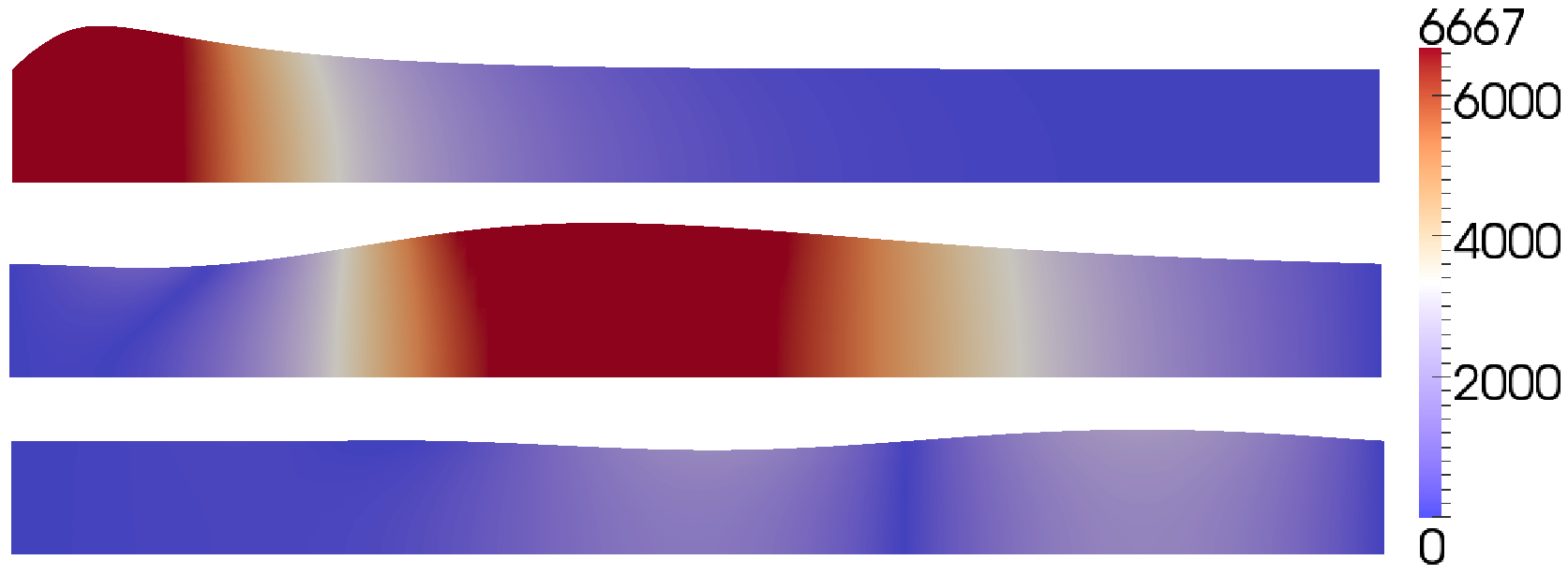
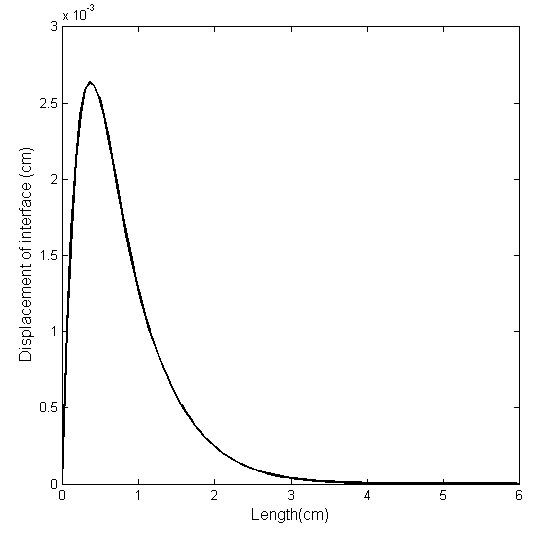
Refer to caption
Figure 2: Pressure surface plot on the deformed 2D fluid domain at times 1.5, 3.5 and 5.5 ms top to bottom. Units are Pa𝑃𝑎Pa. The propagation of a wave is clearly visible. For visualization purposes, the deformation of the domain is magnified 100 times.
Refer to caption
Refer to caption
Refer to caption
Refer to caption
Refer to caption
Refer to caption
Figure 3: Top panel: displacement of the fluid-structure interface at times 1.5, 3.5 and 5.5 ms from left to right. Bottom panel: intramural flow 𝒒h𝒏subscript𝒒𝒏\boldsymbol{q}_{h}\cdot\boldsymbol{n} at different planes in the arterial wall, located at the interface, at the intermediate section and at the outer layer.

Finite element approximation.

The proposed scheme is rather flexible with respect to the definition of the finite element spaces for each unknown, namely 𝐕hf,Qhf,𝐕hp,Qhp,𝐗hp,𝐗˙hpsuperscriptsubscript𝐕𝑓superscriptsubscript𝑄𝑓superscriptsubscript𝐕𝑝superscriptsubscript𝑄𝑝superscriptsubscript𝐗𝑝superscriptsubscript˙𝐗𝑝\mathbf{V}_{h}^{f},\,Q_{h}^{f},\,\mathbf{V}_{h}^{p},\,Q_{h}^{p},\,\mathbf{X}_{h}^{p},\,\dot{\mathbf{X}}_{h}^{p} previously introduced. Owing to the weak enforcement of the interface conditions, in principle it does not require any restriction on the choice of the discrete approximation spaces on each side of the interface, provided that appropriate quadrature methods are adopted to calculate the integrals of test functions evaluated at the interface. Considering the heterogeneous nature of the equations that are coupled though the interface conditions, this is an interesting property of the scheme. Nevertheless, in the forthcoming numerical experiments we will consider some simple choices. To facilitate the exchange of information across the interface, we use the same finite elements for the approximation of the unknowns 𝒗h,𝒒h,𝑼hsubscript𝒗subscript𝒒subscript𝑼\boldsymbol{v}_{h},\,\boldsymbol{q}_{h},\,\boldsymbol{U}_{h} that are combined in the interface conditions, see for example equation (13).

One of the drawbacks of using the Nitsche’s method for interface conditions is that the stability of the scheme relies on the appropriate quantification of the penalty and stabilization operators, namely γf,γstab,γstabsubscript𝛾𝑓subscript𝛾𝑠𝑡𝑎𝑏superscriptsubscript𝛾𝑠𝑡𝑎𝑏\gamma_{f},\,\gamma_{stab},\,\gamma_{stab}^{\prime}. More precisely, these parameters must satisfy the requirements of Theorem 2 or Corollaries 1 and 2, where the explicit expression of the constant CTIsubscript𝐶𝑇𝐼C_{TI} may not be available in general, but only their order of magnitude can be reasonably quantified. As a result, γf,γstab,γstabsubscript𝛾𝑓subscript𝛾𝑠𝑡𝑎𝑏superscriptsubscript𝛾𝑠𝑡𝑎𝑏\gamma_{f},\,\gamma_{stab},\,\gamma_{stab}^{\prime} should be manually tuned for each specific application. For the particular case of FSI related to blood flow in arteries, the sensitivity of the numerical solution on γfsubscript𝛾𝑓\gamma_{f} and γstabsubscript𝛾𝑠𝑡𝑎𝑏\gamma_{stab} has been carefully addressed in [6] for a scheme similar to the one addressed here. According to these results combined with the insight provided by Corollary 2 on the choice of γstabsuperscriptsubscript𝛾𝑠𝑡𝑎𝑏\gamma_{stab}^{\prime}, we have used the following values: γf=2500subscript𝛾𝑓2500\gamma_{f}=2500, γstab=1subscript𝛾𝑠𝑡𝑎𝑏1\gamma_{stab}=1, γstab=0superscriptsubscript𝛾𝑠𝑡𝑎𝑏0\gamma_{stab}^{\prime}=0.

Convergence analysis.

The objective of this section is to support the theoretical results on the accuracy of the proposed scheme, given in Theorem 3. The available theory shows that the main shortcomings of the scheme in terms of accuracy arise in the time approximation and are related to the splitting of the equations within each time step. For this reason, we limit our investigation to the variation of the time step τ𝜏\tau. As reference solution, since the analytical one is not available in this case, we use the numerical solution calculated using the monolithic scheme with a small time step equal to τ=106𝜏superscript106\tau=10^{-6} s. This way, we make sure that the splitting error is not polluting the solution, and the approximation error related to the time discretization scheme is negligible. This solution will be denoted with the subscript ref𝑟𝑒𝑓ref. To guarantee a sufficient spatial resolution as well as inf-sup stability, we use 21superscript2superscript1\mathbb{P}^{2}-\mathbb{P}^{1} approximations for velocity and pressure in the blood flow, combined with 21superscript2superscript1\mathbb{P}^{2}-\mathbb{P}^{1} approximation of Darcy’s equation and 2superscript2\mathbb{P}^{2} approximation of the structure displacement and velocity. We investigate the convergence properties of the scheme in the norm ||||||,N2|||\cdot|||_{\heartsuit,\,N}^{2} that is used in Theorem 3. More precisely, we split it in four parts:

f,hN:=ρf𝒗hN𝒗hN,refL2(Ωf)2,p,hN(a):=ρp𝑼˙hN𝑼˙hN,refL2(Ωp)2,p,hN(c):=s0pp,hNpp,hN,refL2(Ωp)2,formulae-sequenceassignsuperscriptsubscript𝑓𝑁subscript𝜌𝑓subscriptsuperscriptnormsuperscriptsubscript𝒗𝑁superscriptsubscript𝒗𝑁𝑟𝑒𝑓2superscript𝐿2subscriptΩ𝑓formulae-sequenceassignsuperscriptsubscript𝑝𝑁𝑎subscript𝜌𝑝subscriptsuperscriptnormsuperscriptsubscript˙𝑼𝑁superscriptsubscript˙𝑼𝑁𝑟𝑒𝑓2superscript𝐿2subscriptΩ𝑝assignsuperscriptsubscript𝑝𝑁𝑐subscript𝑠0subscriptsuperscriptnormsuperscriptsubscript𝑝𝑝𝑁superscriptsubscript𝑝𝑝𝑁𝑟𝑒𝑓2superscript𝐿2subscriptΩ𝑝\displaystyle\mathcal{E}_{f,h}^{N}:=\rho_{f}\|\boldsymbol{v}_{h}^{N}-\boldsymbol{v}_{h}^{N,ref}\|^{2}_{L^{2}(\Omega_{f})},\ \mathcal{E}_{p,h}^{N}(a):=\rho_{p}\|\dot{\boldsymbol{U}}_{h}^{N}-\dot{\boldsymbol{U}}_{h}^{N,ref}\|^{2}_{L^{2}(\Omega_{p})},\ \mathcal{E}_{p,h}^{N}(c):=s_{0}\|p_{p,h}^{N}-p_{p,h}^{N,ref}\|^{2}_{L^{2}(\Omega_{p})},
p,hN(b):=2μp𝑫(𝑼hN𝑼hN,ref)||L2(Ωp)2+λp(𝑼hN𝑼hN,ref)L2(Ωp)2,assignsuperscriptsubscript𝑝𝑁𝑏evaluated-at2subscript𝜇𝑝delimited-‖|𝑫superscriptsubscript𝑼𝑁superscriptsubscript𝑼𝑁𝑟𝑒𝑓superscript𝐿2subscriptΩ𝑝2subscript𝜆𝑝subscriptsuperscriptnormsuperscriptsubscript𝑼𝑁superscriptsubscript𝑼𝑁𝑟𝑒𝑓2superscript𝐿2subscriptΩ𝑝\displaystyle\mathcal{E}_{p,h}^{N}(b):=2\mu_{p}\|{\boldsymbol{D}}(\boldsymbol{U}_{h}^{N}-\boldsymbol{U}_{h}^{N,ref})||^{2}_{L^{2}(\Omega_{p})}+\lambda_{p}||\nabla\cdot(\boldsymbol{U}_{h}^{N}-\boldsymbol{U}_{h}^{N,ref})||^{2}_{L^{2}(\Omega_{p})},

corresponding to the fluid kinetic energy, the structure kinetic energy, the structure elastic stored energy and the pressure, respectively. We calculate the error between the reference solution and solutions obtained using τ=τ0,τ0/2,τ0/4,τ0/8𝜏subscript𝜏0subscript𝜏02subscript𝜏04subscript𝜏08\tau=\tau_{0},\tau_{0}/2,\tau_{0}/4,\tau_{0}/8 with τ0=104subscript𝜏0superscript104\tau_{0}=10^{-4} for simulations up to the final time T=103𝑇superscript103T=10^{-3} s. The mesh discretization step is h=0.050.05h=0.05 cm for all cases.

monolithic f,hNsuperscriptsubscript𝑓𝑁\sqrt{\mathcal{E}_{f,h}^{N}} rate p,hN(a)superscriptsubscript𝑝𝑁𝑎\sqrt{\mathcal{E}_{p,h}^{N}}(a) rate p,hN(b)superscriptsubscript𝑝𝑁𝑏\sqrt{\mathcal{E}_{p,h}^{N}}(b) rate p,hN(c)superscriptsubscript𝑝𝑁𝑐\sqrt{\mathcal{E}_{p,h}^{N}}(c) rate
τ0=104subscript𝜏0superscript104\tau_{0}=10^{-4} 2.14E-01 1.48E-01 5.24E-01 1.32E-02
τ0/2subscript𝜏02\tau_{0}/2 1.05E-01 1.02 7.89E-02 0.91 2.82E-01 0.90 6.95E-03 0.92
τ0/4subscript𝜏04\tau_{0}/4 5.13E-02 1.04 4.03E-02 0.97 1.44E-01 0.97 3.53E-03 0.98
τ0/8subscript𝜏08\tau_{0}/8 2.45E-02 1.07 1.98E-02 1.03 7.07E-02 1.03 1.72E-03 1.03
partitioned f,hNsuperscriptsubscript𝑓𝑁\sqrt{\mathcal{E}_{f,h}^{N}} rate p,hN(a)superscriptsubscript𝑝𝑁𝑎\sqrt{\mathcal{E}_{p,h}^{N}}(a) rate p,hN(b)superscriptsubscript𝑝𝑁𝑏\sqrt{\mathcal{E}_{p,h}^{N}}(b) rate p,hN(c)superscriptsubscript𝑝𝑁𝑐\sqrt{\mathcal{E}_{p,h}^{N}}(c) rate
τ0=104subscript𝜏0superscript104\tau_{0}=10^{-4} 2.87E-01 1.84E-01 7.71E-01 1.96E-02
τ0/2subscript𝜏02\tau_{0}/2 1.49E-01 0.94 9.91E-02 0.89 4.15E-01 0.90 1.01E-02 0.95
τ0/4subscript𝜏04\tau_{0}/4 7.58E-02 0.98 5.16E-02 0.94 2.13E-01 0.96 5.09E-03 0.99
τ0/8subscript𝜏08\tau_{0}/8 3.75E-02 1.01 2.59E-02 0.99 1.06E-01 1.01 2.49E-03 1.03
Table 2: Convergence in time of the monolithic and the partitioned scheme, respectively.

In Table 2 we show the convergence rate relative to the error indicators above calculated using both the monolithic and the loosely coupled scheme. We observe that, as expected, the error indicators scale as Cτ𝐶𝜏C\tau when the monolithic scheme is used. This result confirms the statement of Assumption 1 with p=1𝑝1p=1, since we use the Backward Euler scheme for the time discretization of all the time dependent equations. Looking at the error of the loosely coupled scheme, we notice that for each of the indicators the magnitude of the error increases with respect to the monolithic scheme. This is the contribution of the splitting error. However, quite surprisingly, we observe that the total error of the loosely coupled scheme scales as Cτ𝐶𝜏C\tau, although Lemma 3 shows that the splitting error should asymptotically behave as C1τh+C2τ2+C3ϑτsubscript𝐶1𝜏subscript𝐶2superscript𝜏2subscript𝐶3italic-ϑ𝜏\sqrt{C_{1}\frac{\tau}{h}+C_{2}\tau^{2}+C_{3}\vartheta\tau}. Combining these observations, we conclude that the splitting error is non negligible, but the dominant term among these three contributions is C2τsubscript𝐶2𝜏\sqrt{C_{2}}\tau. In other words, for the problem at hand, the available results suggest that C2C1,C3much-greater-thansubscript𝐶2𝐶1subscript𝐶3C_{2}\gg C1,\,C_{3}.

The loosely coupled scheme as a preconditioner for the monolithic formulation.

In order to simplify the management of the algebraic degrees of freedom related to the finite element spaces, for this test case we adopt a 11superscript1superscript1\mathbb{P}^{1}-\mathbb{P}^{1} approximations for velocity and pressure respectively. It is well known that this choice does not satisfy the inf-sup stability condition [19, 37]. Resorting to a pressure stabilization method on the whole fluid domain is mandatory. Owing to its simplicity of implementation, we opt for the Brezzi-Pitkaranta scheme [2], that is

sp(pf,hn,ψf,h):=γph2Ωfpf,hnψf,hd𝒙,assignsubscript𝑠𝑝superscriptsubscript𝑝𝑓𝑛subscript𝜓𝑓subscript𝛾𝑝superscript2subscriptsubscriptΩ𝑓superscriptsubscript𝑝𝑓𝑛subscript𝜓𝑓𝑑𝒙s_{p}(p_{f,h}^{n},\psi_{f,h}):=\gamma_{p}h^{2}\int_{\Omega_{f}}\nabla p_{f,h}^{n}\cdot\nabla\psi_{f,h}d\boldsymbol{x},

where the stabilization parameter is selected as γp=102subscript𝛾𝑝superscript102\gamma_{p}=10^{-2} on the basis of numerical experiments. The same type of spaces are used for the intramural filtration and pressure, namely 𝒒h,pp,hsubscript𝒒subscript𝑝𝑝\boldsymbol{q}_{h},p_{p,h}. Since equation (7) is not enforcing the divergence-free constraint exactly, but the material turns out to be slightly compressible, equal order approximation is stable. We also use 1superscript1\mathbb{P}^{1} finite elements to approximate the structure velocity and displacement.

Equation (40) suggests that the partitioned scheme may act as an efficient preconditioner for the monolithic equation. On one hand, the corresponding matrices share similar spectral properties. On the other hand, the computational cost of solving the partitioned scheme is significantly lower than the one related to the monolithic formulation. Indeed, matrix A^hsubscript^A\widehat{\mathrm{A}}_{h} features a block upper triangular structure that enables us to solve the structure, Darcy and blood flow problems independently. The performance of matrix A^hsubscript^A\widehat{\mathrm{A}}_{h} used as a preconditioner of A~hssuperscriptsubscript~A𝑠\widetilde{\mathrm{A}}_{h}^{s} is quantified by the numerical experiments reported in Table 3. As an indicator of the system conditioning, we look at the number of GMRES iterations required to reduce below a given tolerance the relative residual, defined as the left hand side of (41). In the special case of positive definite matrices, a manipulation of (41) allows us to show that the number of iterations (# GMRES) required to reduce the relative residual of a factor 10psuperscript10𝑝10^{p}, can be estimated as # GMRES p(K(P1A))similar-to-or-equalsabsent𝑝𝐾superscript𝑃1𝐴\simeq p\sqrt{\big{(}K(P^{-1}A)\big{)}}, where K()𝐾K(\cdot) is the spectral condition number. Since the initial relative residual is one, by definition, (# GMRES) is equivalent to the number of iterations performed until the relative residual is less than 10psuperscript10𝑝10^{-p}. In the experiments that follow, we have used p=6𝑝6p=6. As a result, knowing that the conditioning of the FEM stiffness matrices scales as the square of the number of degrees of freedom, we expect that # GMRES linearly scales with the number of degrees of freedom in absence of preconditioners. Optimal preconditioners are those where the number of GMRES iterations becomes independent of the dimension of the discrete problem.

Artery test case (i𝑖i)

τ=104𝜏superscript104\tau=10^{-4} h=0.050.05h=0.05 h=0.0250.025h=0.025 h=0.01250.0125h=0.0125
# GMRES(A~hssuperscriptsubscript~A𝑠\widetilde{\mathrm{A}}_{h}^{s}) 211.4 446.4 1282.9
# GMRES((A^h)1A~hssuperscriptsubscript^A1superscriptsubscript~A𝑠(\widehat{\mathrm{A}}_{h})^{-1}\widetilde{\mathrm{A}}_{h}^{s}) 10.9 12 13.9

Artery test case (i𝑖i)

τ=105𝜏superscript105\tau=10^{-5} h=0.050.05h=0.05 h=0.0250.025h=0.025 h=0.01250.0125h=0.0125
# GMRES(A~hssuperscriptsubscript~A𝑠\widetilde{\mathrm{A}}_{h}^{s}) 362.1 498.3 1194.4
# GMRES((A^h)1A~hssuperscriptsubscript^A1superscriptsubscript~A𝑠(\widehat{\mathrm{A}}_{h})^{-1}\widetilde{\mathrm{A}}_{h}^{s}) 8 10 12.9

Fractured reservoir test case (ii𝑖𝑖ii)

τ=103𝜏superscript103\tau=10^{-3} h=1.061.06h=1.06 h=0.4500.450h=0.450 h=0.2120.212h=0.212
# GMRES(A~hssuperscriptsubscript~A𝑠\widetilde{\mathrm{A}}_{h}^{s}) 53.8 101.7 245.4
# GMRES((A^h)1A~hssuperscriptsubscript^A1superscriptsubscript~A𝑠(\widehat{\mathrm{A}}_{h})^{-1}\widetilde{\mathrm{A}}_{h}^{s}) 2 2 2
Table 3: Average number of GMRES iterations (# GMRES) required to reduce the relative residual of a factor 106superscript10610^{-6}. The values are calculated on the basis of the first 10 time steps of the simulation.

The results of Table 3 nicely agree with the general GMRES convergence theory, namely Theorem 4, and confirm that A^hsubscript^A\widehat{\mathrm{A}}_{h} behaves as an optimal preconditioner for A~hssuperscriptsubscript~A𝑠\widetilde{\mathrm{A}}_{h}^{s}. Not only the number of iterations to solve the preconditioned system is nearly insensitive with respect to the mesh characteristic size, and consequently the number of degrees of freedom of the discrete problem, but the number of iterations is significantly smaller than in the non preconditioned case. Reminding that the inversion of A^hsubscript^A\widehat{\mathrm{A}}_{h} is a relatively inexpensive operation, the preconditioned algorithm turns out to be a very effective solution method. Table 3 also suggests that the conditioning of the monolithic problem slightly increases when the time step is refined, especially for coarse meshes, while the good preconditioner performance seems to be unaffected. It indeed slightly improves, according to the fact that the loosely coupled scheme, and the related preconditioner, becomes more accurate and effective when the time discretization step decreases. We have tested this algorithm also using quadratic finite elements, 2superscript2\mathbb{P}^{2}, for all velocities and displacement fields. In the case of the coarsest mesh h=0.050.05h=0.05 cm, GMRES converges in 613.5 (average) iterations, while solving the preconditioned only requires 11 iterations. The preconditioner seems to scale well also with respect to the FEM polynomial degree. The good results on preconditioner performance also correspond to a decrease in the computational time. For h=0.05,τ=104formulae-sequence0.05𝜏superscript104h=0.05,\,\tau=10^{-4}, the calculation of 606060 time steps of the monolithic scheme require 4.73 seconds, while for the preconditioned method the time is 1.85 seconds. For τ=104𝜏superscript104\tau=10^{-4} and 600600600 time steps the computational times are respectively, 65.8 seconds and 14.6 seconds. Finally, we observe that these considerations apply also to the test case (ii𝑖𝑖ii), addressed in the next section, which represents a prototype problem for flow though a fractured reservoir.

5.2 Application of the scheme to flow through fractured reservoirs

In this example we focus on fluid-structure interaction in the context of modelling the interaction between a stationary fracture filled with fluid and the surrounding poroelastic medium. We consider a general case where the hydraulic conductivity is a tensor given by 𝜿=𝑲μf𝜿𝑲subscript𝜇𝑓\boldsymbol{\kappa}=\frac{\boldsymbol{K}}{\mu_{f}}, where 𝑲𝑲\boldsymbol{K} is the permeability tensor. Since the effect of the porous media on the conduit flow at the interface is more prominent in this application, we replace the no-slip condition (14) by the Beavers-Joseph-Saffman condition (15) with the coefficient

β=(αμf3tr(𝑲))1.𝛽superscript𝛼subscript𝜇𝑓3tr𝑲1\beta=\left(\frac{\alpha\mu_{f}\sqrt{3}}{\sqrt{\textrm{tr}(\boldsymbol{K})}}\right)^{-1}. (42)

We consider 2D and 3D test cases. In 2D, our reference domain is a square [100,100]2superscript1001002[-100,100]^{2} m. A fracture is positioned in the middle of the square, whose boundary is given by

y^2=0.0082(x^35)2(x^+352).superscript^𝑦2superscript0.0082superscript^𝑥352^𝑥superscript352\hat{y}^{2}=0.008^{2}(\hat{x}-35)^{2}(\hat{x}+35^{2}).

The fracture represents the reference fluid domain Ω^fsuperscript^Ω𝑓\hat{\Omega}^{f}, while the reference poroelastic structure domain is given as Ω^p=Ω^\Ω^f.superscript^Ω𝑝\^Ωsuperscript^Ω𝑓\hat{\Omega}^{p}=\hat{\Omega}\backslash\hat{\Omega}^{f}. Following the approach in [23], to obtain a more realistic domain, we transform the reference domain Ω^^Ω\hat{\Omega} onto the physical domain ΩΩ\Omega via the mapping

[xy](x^,y^)=[x^5cos(x^+y^100)cos(πx^+y^100)2+y^/5x^/10].\left[\begin{array}[]{c}x\\ y\end{array}\right](\hat{x},\hat{y})=\left[\begin{array}[]{c}\hat{x}\\ 5\cos\left(\displaystyle\frac{\hat{x}+\hat{y}}{100}\right)\cos\left(\displaystyle\frac{\pi\hat{x}+\hat{y}}{100}\right)^{2}+\hat{y}/5-\hat{x}/10\end{array}\right]. (43)

The extension to the 3D test case consists of introducing a reference domain Ω^=Ω^fΩ^p^Ωsuperscript^Ω𝑓superscript^Ω𝑝\hat{\Omega}=\hat{\Omega}^{f}\cup\hat{\Omega}^{p} which is a cube [100,100]3superscript1001003[-100,100]^{3} m. A circular fracture with radius of 353535 m and maximum height of 202020 m is positioned in the middle of the cube. Then, we apply the mapping

[xyz](x^,y^,z^)=[x^5cos(πz^+x^+y^100)cos(πx^+y^100)2+y^/5+x^(z^/1001)/10z^].\left[\begin{array}[]{c}x\\ y\\ z\end{array}\right](\hat{x},\hat{y},\hat{z})=\left[\begin{array}[]{c}\hat{x}\\ 5\cos\left(\displaystyle\frac{\pi\hat{z}+\hat{x}+\hat{y}}{100}\right)\cos\left(\displaystyle\frac{\pi\hat{x}+\hat{y}}{100}\right)^{2}+\hat{y}/5+\hat{x}(\hat{z}/100-1)/10\\ \hat{z}\end{array}\right]. (44)

Figure 4 shows the physical domain ΩΩ\Omega in 2D (left) and 3D (right).

Refer to caption
Figure 4: Left: Physical computational domain Ω=ΩfΩpΩsuperscriptΩ𝑓superscriptΩ𝑝\Omega=\Omega^{f}\cup\Omega^{p} in 2D. Middle: Physical domain ΩpsuperscriptΩ𝑝\Omega^{p} in 3D. Right: Physical domain ΩfsuperscriptΩ𝑓\Omega^{f} in 3D.

The flow is driven by the injection of the fluid into the fracture with the constant rate g=25𝑔25g=25 kg/s. The fluid is injected into a circle (2D) or a cube (3D) of radius 777 m in the center of the reference fracture Ω^fsuperscript^Ω𝑓\hat{\Omega}^{f}. On all external boundaries, we prescribe the no flow condition 𝒒𝒏=0𝒒𝒏0\boldsymbol{q}\cdot\boldsymbol{n}=0, zero normal displacement 𝑼𝒏=0𝑼𝒏0\boldsymbol{U}\cdot\boldsymbol{n}=0, and zero shear traction 𝒕𝝈f𝒏=0𝒕subscript𝝈𝑓𝒏0\boldsymbol{t}\cdot\boldsymbol{\sigma}_{f}\boldsymbol{n}=0. The computational time is T=5.1𝑇5.1T=5.1 hours. The problem was solved using the time step Δt=0.1Δ𝑡0.1\Delta t=0.1 seconds. The remaining parameters are given in Table 4. These parameters are similar to the ones in [23], and are taken to be within realistic range for applications to hydraulic fracturing.

Parameter Symbol Units Value
Poroelastic wall density ρpsubscript𝜌𝑝\rho_{p} (kg/m3) 897897897
Fluid density ρfsubscript𝜌𝑓\rho_{f} (kg/m3) 897897897
Dyn. viscosity μ𝜇\mu (Pa s) 103superscript10310^{-3}
Lamé coeff. μpsubscript𝜇𝑝\mu_{p} (Pa) 2.92×10102.92superscript10102.92\times 10^{10}
Lamé coeff. λpsubscript𝜆𝑝\lambda_{p} (Pa) 1.94×10101.94superscript10101.94\times 10^{10}
Hydraulic conductivity (2D) 𝜿𝜿\boldsymbol{\kappa} (m2/Pa s) diag(200,50)×1012𝑑𝑖𝑎𝑔20050superscript1012diag(200,50)\times 10^{-12}
Hydraulic conductivity (3D) 𝜿𝜿\boldsymbol{\kappa} (m2/Pa s) diag(200,50,200)×1012𝑑𝑖𝑎𝑔20050200superscript1012diag(200,50,200)\times 10^{-12}
Mass storativity coeff. s0subscript𝑠0s_{0} (Pa-1) 6.9×1056.9superscript1056.9\times 10^{-5}
Biot-Willis constant α𝛼\alpha 1
Beavers-Joseph-Saffman coefficient (2D) β𝛽\beta (m2/Pa s) 2.881042.88superscript1042.88\cdot 10^{-4}
Beavers-Joseph-Saffman coefficient (3D) β𝛽\beta (m2/Pa s) 3.881043.88superscript1043.88\cdot 10^{-4}
Total simulation time T𝑇T (s) 186001860018600
Table 4: Fluid and structure parameters.

In the 2D case, we use the conforming meshes for the discretization of the fluid and structure domains. In 3D case, we exploit the weak enforcement of the interface conditions and use non-conforming computational meshes. We use the preconditioned monolithic numerical solver. Its implementation in FreeFem++ facilitates the interpolation of finite element functions across the interface. We adopt the 11superscript1superscript1\mathbb{P}^{1}-\mathbb{P}^{1} approximation for the fluid velocity and pressure, complemented with the pressure stabilization sp(pf,h,ψf,h)subscript𝑠𝑝subscript𝑝𝑓subscript𝜓𝑓s_{p}(p_{f,h},\psi_{f,h}). For the Darcy fluid-pressure approximation in the poroelastic medium, as for the structure velocity and displacement, we again use the 11superscript1superscript1\mathbb{P}^{1}-\mathbb{P}^{1} finite elements. However, due to the large time-step in this example, we are numerically closer to the divergence-free regime. Thus, we add a Darcy pressure stabilization given by

sq(pp,h,ψp,h)=γqh2Ωppp,hψp,hd𝒙,subscript𝑠𝑞subscript𝑝𝑝subscript𝜓𝑝subscript𝛾𝑞superscript2subscriptsubscriptΩ𝑝subscript𝑝𝑝subscript𝜓𝑝𝑑𝒙s_{q}(p_{p,h},\psi_{p,h})=\gamma_{q}h^{2}\int_{\Omega_{p}}\nabla p_{p,h}\cdot\nabla\psi_{p,h}d\boldsymbol{x},

where the stabilization parameter is selected as γq=103subscript𝛾𝑞superscript103\gamma_{q}=10^{-3}. Finally, the choice of the penalty and stabilization parameters is γf=1500subscript𝛾𝑓1500\gamma_{f}=1500, γstab=1subscript𝛾𝑠𝑡𝑎𝑏1\gamma_{stab}=1, γstab=0superscriptsubscript𝛾𝑠𝑡𝑎𝑏0\gamma_{stab}^{\prime}=0.

The visualization of the injection of the fluid into the fracture, and the fluid leakoff to the surrounding rock at the final time T𝑇T is shown in a sequence of Figures, numbered from 5 to 10.

Refer to caption
Refer to caption
Figure 5: Top: Fluid pressure in 2D (left) and a slice of the pressure in the middle of the fracture in 3D (right) at final time T𝑇T. Bottom: Fluid velocity in 2D (left) and and a slice of the velocity in the middle of the fracture in 3D (right) at final time T𝑇T.
Refer to caption
Refer to caption
Figure 6: Fluid pressure in 3D at time t=5𝑡5t=5 seconds (left) and at the final time T𝑇T (right).
Refer to caption
Figure 7: Fluid velocity in the surrounding medium in 2D (left) and 3D (right) at final time T𝑇T.
Refer to caption
Refer to caption
Figure 8: Fluid pressure (left) and displacement (right) in surrounding medium in 2D at final time T𝑇T.
Refer to caption
Figure 9: Top: Pressure in the poroelastic medium at final time T𝑇T. Bottom: Displacement in the poroelastic medium at final time T𝑇T.
Refer to caption
Figure 10: Displacement of the poroelastic medium in 3D in the vertical (left) and axial (right) direction at final time T𝑇T.

Figure 5 shows the pressure (top) and the velocity (bottom) in the fracture for the 2D (left) and 3D (right) test cases, at final time T𝑇T. The 3D plots are obtained by taking a slice through the center of the domain. A top view of the fluid pressure in the fracture is shown in Figure 6 (as the pressure range is very narrow in the right panel, small mesh dependent fluctuations of the pressure are visible from the pressure contour plot). At the beginning of the process the simulations capture the expected local pressure increase in the region of fluid injection, while at the final time, the fluid pressure is the largest at the tip of the crack in both 2D and 3D test cases. Figure 7 shows the comparison of Darcy velocity in the surrounding medium obtained in 2D (left) and 3D (right) at final time T𝑇T. Pressure and displacement are shown in the surrounding medium, in the 2D case in Figure 8, and in the 3D test case in Figure 9. Finally, the displacement of the surrounding medium in the vertical (left) and axial (right) direction is shown in Figure 10.

This example demonstrates the ability of our algorithm to handle complex, three-dimensional simulations in different applications. Retaining the advantages of a monolithic scheme, the computational time is significantly reduced due to a well-designed preconditioner. Our model includes Darcy equations in the mixed formulation which are necessary to compute accurately the Darcy velocity in the surrounding rock. Furthermore, we are able to capture displacement of the fracture which has a complex, very slender domain with sharp edges.

6 Conclusions

We have studied the interaction of a free fluid with a poroelastic material. After setting appropriate governing equations on adjacent domains and discussing the corresponding interface conditions, we have considered the discretization of the problem in the framework of the finite element method. Particular attention must be devoted to the approximation of the interface conditions, which are non standard with respect to the ones that arise in the coupling of homogenous partial differential equations. We have shown that the Nitsche’s method, well known the weak approximation of boundary and interface conditions for elliptic or parabolic problems, is very appropriate to enforce the interface constraints in the variational formulation. The resulting discrete, fully coupled problem features good stability properties. Since all the interface conditions correspond to suitable operators in the variational problem, time-lagging allows to split the fully coupled problem into subproblems, relative to the main governing equations, such as free fluid flow, Darcy filtration and elastodynamics. Also the resulting loosely coupled problem formulation turns out to be stable, provided that it is combined with suitable stabilization operators. This solution approach is very effective from the computational standpoint, but suffers from low accuracy, as we have pointed out in the error analysis of the scheme. In order to merge the computational efficiency of the loosely coupled scheme with the good accuracy and stability properties of the monolithic formulation, we develop a numerical solver where the former scheme acts as a preconditioner for the latter. The theory and the numerical results suggest that this approach is very effective because the loosely coupled scheme behaves as an optimal preconditioner for the monolithic formulation. This solution algorithm turns out to be very robust with respect to the characteristic physical parameters of the problem. Indeed, we have successfully applied it to the analysis of a problem related to blood flow in arteries as well as to the study of subsurface flow and deformation of a fractured reservoir.

References

References

  • [1] S. Badia, A. Quaini, and A. Quarteroni. Coupling Biot and Navier–Stokes equations for modelling fluid–poroelastic media interaction. Journal of Computational Physics, 228(21):7986–8014, 2009.
  • [2] F. Brezzi and J. Pitkäranta. On the stabilization of finite element approximations of the Stokes equations. In Efficient solutions of elliptic systems (Kiel, 1984), volume 10 of Notes Numer. Fluid Mech., pages 11–19. Vieweg, Braunschweig, 1984.
  • [3] M. Bukač, S. Čanić, R. Glowinski, J. Tambača, and A. Quaini. Fluid-structure interaction in blood flow capturing non-zero longitudinal structure displacement. Journal of Computational Physics, 2012.
  • [4] Martina Bukac, Paolo Zunino, and Ivan Yotov. Explicit partitioning strategies for the interaction between a fluid and a multilayered poroelastic structure: an operator-splitting approach. arXiv preprint arXiv:1308.4454, 2013.
  • [5] M. Bukač, W. Layton, M. Moraiti, H. Trang, and C. Trenchea. Analysis of partitioned methods for biot system. Technical report, 2013. Submitted.
  • [6] E. Burman and M.A. Fernández. Stabilization of explicit coupling in fluid-structure interaction involving fluid incompressibility. Comput. Methods Appl. Mech. Engrg., 198(5-8):766–784, 2009.
  • [7] E. Burman and M.A. Fernández. Explicit strategies for incompressible fluid-structure interaction problems: Nitsche type mortaring versus Robin-Robin coupling. International Journal for Numerical Methods in Engineering, pages n/a–n/a, 2013.
  • [8] Y. Cao, M. Gunzburger, X. Hu, F. Hua, X. Wang, and W. Zhao. Finite element approximations for Stokes-Darcy flow with Beavers-Joseph interface conditions. SIAM Journal on Numerical Analysis, 47(6):4239–4256, 2010.
  • [9] Y. Cao, M. Gunzburger, F. Hua, and X. Wang. Coupled stokes-darcy model with beavers-joseph interface boundary condition. Communications in Mathematical Sciences, 8(1):1–25, 2010.
  • [10] P. Causin, J.F. Gerbeau, and F. Nobile. Added-mass effect in the design of partitioned algorithms for fluid-structure problems. Comput. Methods Appl. Mech. Eng., 194(42-44):4506–4527, 2005.
  • [11] Aycil Cesmelioglu, Vivette Girault, and Béatrice Rivière. Time-dependent coupling of Navier-Stokes and Darcy flows. ESAIM Math. Model. Numer. Anal., 47(2):539–554, 2013.
  • [12] Jeffrey M. Connors and Jason S. Howell. A fluid-fluid interaction method using decoupled subproblems and differing time steps. Numer. Methods Partial Differential Equations, 28(4):1283–1308, 2012.
  • [13] Jeffrey M. Connors, Jason S. Howell, and William J. Layton. Decoupled time stepping methods for fluid-fluid interaction. SIAM J. Numer. Anal., 50(3):1297–1319, 2012.
  • [14] Carlo D’Angelo and Paolo Zunino. A finite element method based on weighted interior penalties for heterogeneous incompressible flows. SIAM J. Numer. Anal., 47(5):3990–4020, 2009.
  • [15] Carlo D’Angelo and Paolo Zunino. Numerical approximation with Nitsche’s coupling of transient Stokes’/Darcy’s flow problems applied to hemodynamics. Appl. Numer. Math., 62(4):378–395, 2012.
  • [16] M. Discacciati, E. Miglio, and A. Quarteroni. Mathematical and numerical models for coupling surface and groundwater flows. Appl. Numer. Math., 43(1-2):57–74, 2002.
  • [17] J. Donea, S. Giuliani, and J.P. Halleux. An arbitrary lagrangian-eulerian finite element method for transient dynamic fluid-structure interactions. Computer Methods in Applied Mechanics and Engineering, 33(1-3):689–723, 1982.
  • [18] Stanley C. Eisenstat, Howard C. Elman, and Martin H. Schultz. Variational iterative methods for nonsymmetric systems of linear equations. SIAM Journal on Numerical Analysis, 20(2):345–357, April 1983.
  • [19] Alexandre Ern and Jean-Luc Guermond. Theory and practice of finite elements, volume 159 of Applied Mathematical Sciences. Springer-Verlag, New York, 2004.
  • [20] C. Förster, W.A. Wall, and E. Ramm. Artificial added mass instabilities in sequential staggered coupling of nonlinear structures and incompressible viscous flows. Computer Methods in Applied Mechanics and Engineering, 196(7):1278–1293, 2007.
  • [21] B. Ganis, M. Mear, A. Sakhaee-Pour, M.F. Wheeler, and T. Wick. Modeling fluid injection in fractures with a reservoir simulator coupled to a boundary element method. Computational Geosciences, 2013. To appear.
  • [22] Benjamin Ganis, Vivette Girault, Mark Mear, Gurpreet Singh, and Mary F. Wheeler. Modeling fractures in a poro-elastic medium. Technical Report 09, The Institute for Computational Engineering and Sciences (ICES), The University of Texas, Austin., 2013.
  • [23] Vivette Girault, Mary F. Wheeler, Benjamin Ganis, and Mark E. Mear. A lubrication fracture model in a poro-elastic medium. Technical Report 32, The Institute for Computational Engineering and Sciences (ICES), The University of Texas, Austin., 2013.
  • [24] P. Hansbo. Nitsche’s method for interface problems in computational mechanics. GAMM-Mitt., 28(2):183–206, 2005.
  • [25] F. Hecht. New development in freefem++. J. Numer. Math., 20(3-4):251–265, 2012.
  • [26] J.M. Kennedy and T.B. Belytschko. Theory and application of a finite element method for arbitrary lagrangian-eulerian fluids and structures. Nuclear Engineering and Design, 68(2):129–146, 1982.
  • [27] J. Kim, H. A. Tchelepi, and R. Juanes. Stability and convergence of sequential methods for coupled flow and geomechanics: drained and undrained splits. Comput. Methods Appl. Mech. Engrg., 200(23-24):2094–2116, 2011.
  • [28] William Layton, Hoang Tran, and Catalin Trenchea. Analysis of long time stability and errors of two partitioned methods for uncoupling evolutionary groundwater-surface water flows. SIAM J. Numer. Anal., 51(1):248–272, 2013.
  • [29] W.J. Layton, F. Schieweck, and I. Yotov. Coupling fluid flow with porous media flow. SIAM Journal on Numerical Analysis, 40(6):2195–2218, 2002.
  • [30] Matteo Lesinigo, Carlo D’Angelo, and Alfio Quarteroni. A multiscale Darcy-Brinkman model for fluid flow in fractured porous media. Numer. Math., 117(4):717–752, 2011.
  • [31] X. Ma, GC.. Lee, and S.G. Wu. Numerical simulation for the propagation of nonlinear pulsatile waves in arteries. Journal of biomechanical engineering, 114:490, 1992.
  • [32] Vincent Martin, Jérôme Jaffré, and Jean E. Roberts. Modeling fractures and barriers as interfaces for flow in porous media. SIAM J. Sci. Comput., 26(5):1667–1691 (electronic), 2005.
  • [33] Andro Mikelić and Mary F. Wheeler. On the interface law between a deformable porous medium containing a viscous fluid and an elastic body. Math. Models Methods Appl. Sci., 22(11):1250031, 32, 2012.
  • [34] Andro Mikelić and Mary F. Wheeler. Convergence of iterative coupling for coupled flow and geomechanics. Comput. Geosci., 17(3):455–461, 2013.
  • [35] Olivier Pironneau, Frédéric Hecht, and Jacques Morice. freeFEM++, www.freefem.org/.
  • [36] A. Quaini. Algorithms for fluid-structure interaction problems arising in hemodynamics. PhD thesis, EPFL, Switzerland, 2009.
  • [37] Alfio Quarteroni and Alberto Valli. Numerical approximation of partial differential equations, volume 23 of Springer Series in Computational Mathematics. Springer-Verlag, Berlin, 1994.
  • [38] B. Rivière and I. Yotov. Locally conservative coupling of Stokes and Darcy flows. SIAM Journal on Numerical Analysis, 42(5):1959–1977, 2005.
  • [39] Ralph E. Showalter. Poroelastic filtration coupled to Stokes flow. In Control theory of partial differential equations, volume 242 of Lect. Notes Pure Appl. Math., pages 229–241. Chapman & Hall/CRC, Boca Raton, FL, 2005.
  • [40] Joshua A. White and Ronaldo I. Borja. Block-preconditioned Newton-Krylov solvers for fully coupled flow and geomechanics. Comput. Geosci., 15(4):647–659, 2011.