Iterative Learning for Reference-Guided DNA Sequence Assembly from Short Reads: Algorithms and Limits of Performance

Abstract

Recent emergence of next-generation DNA sequencing technology has enabled acquisition of genetic information at unprecedented scales. In order to determine the genetic blueprint of an organism, sequencing platforms typically employ so-called shotgun sequencing strategy to oversample the target genome with a library of relatively short overlapping reads. The order of nucleotides in the reads is determined by processing the acquired noisy signals generated by the sequencing instrument. Assembly of a genome from potentially erroneous short reads is a computationally daunting task even in the scenario where a reference genome exists. Errors and gaps in the reference, and perfect repeat regions in the target, further render the assembly challenging and cause inaccuracies. In this paper, we formulate the reference-guided sequence assembly problem as the inference of the genome sequence on a bipartite graph and solve it using a message-passing algorithm. The proposed algorithm can be interpreted as the well-known classical belief propagation scheme under a certain prior. Unlike existing state-of-the-art methods, the proposed algorithm combines the information provided by the reads without needing to know reliability of the short reads (so-called quality scores). Relation of the message-passing algorithm to a provably convergent power iteration scheme is discussed. To evaluate and benchmark the performance of the proposed technique, we find an analytical expression for the probability of error of a genie-aided maximum a posteriori (MAP) decision scheme. Results on both simulated and experimental data demonstrate that the proposed message-passing algorithm outperforms commonly used state-of-the-art tools, and it nearly achieves the performance of the aforementioned MAP decision scheme.

I Introduction

In the last decade, rapid development of next-generation DNA sequencing technologies has enabled cheap and fast generation of massive amounts of sequencing data [1, 2, 3]. Determining the order of nucleotides in a long target DNA molecule typically involves use of shotgun sequencing strategy where multiple copies of the target are fragmented into short templates. Each template is then analyzed by a sequencing instrument which provides reads (i.e., information about nucleotide content of the templates) that are used to assemble the desired long sequence. Shotgun sequencing strategy is illustrated in Fig. 1.

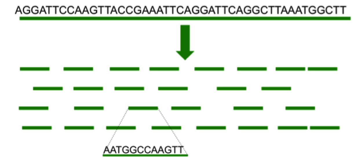
Figure 1: Illustration of shotgun sequencing. Multiple copies of a long target DNA molecule are fragmented into short templates. The order of bases in the templates (reads) is determined using a sequencing instrument, and the reads are then used to assemble the target.

The majority of next-generation sequencing methods detect the order of nucleotides in a template by facilitating enzymatic synthesis of a complementary strand on the template, and acquiring a signal that indicates the type of a nucleotide successfully incorporated into the complementary strand. Quality of the acquired signal is adversely affected by various sources of uncertainty. Base calling algorithms attempt to infer the order of nucleotides in short templates from the acquired noisy signals [4]. Confidence in the accuracy of base calls is expressed by their quality scores, which provide a measure of the probability of base calling error. Conventional base calling algorithms rely on various heuristics to estimate quality scores, while more recent methods employ Bayesian inference schemes to evaluate posteriori probabilities of the bases in the reads [5, 6, 7]. Due to their computational efficiency, the heuristic methods are the preferred choice for assessing confidence of the base calls – however, the resulting quality scores are not necessarily an accurate reflection of the actual probability of base calling errors [8]. In turn, inaccurate quality scores may adversely impact reliability of the assembly process.

The short reads generated by a sequencing instrument are used to assemble the target genome. The assembly may be performed with or without referring to a previously determined sequence related to the target (genome, transcriptome, proteins). De novo assembly refers to a scenario where the reconstruction is performed without a reference sequence. This is a computationally challenging task, difficult due to the presence of perfect repeat regions in the target sequence and short lengths of the reads [11], [12]. In re-sequencing projects where the goal, for instance, may be to study genetic variations among individuals or to discover new strains of bacteria [9], [10], a reference is available and used to order the reads. Such reference-guided assembly is still challenging due to the errors in the reads and because the reference often contains errors and gaps [13], [14]. Many of the assembly challenges are ameliorated if the target sequence is significantly oversampled and thus the information provided by short reads is highly redundant. This redundancy is quantified by means of a sequencing coverage – the average number of times a base in the target sequence is present in the overlapping reads. However, the demands for higher throughput and lower sequencing costs often limit the coverage to medium (5-20X) or low ($\leq 5$X). As an example, the ongoing 1000 Genomes Project has opted for trading-off sequencing depth for the number of individuals being sequenced [18]. In its preliminary phase, the project has focused on sequencing a large number of individuals at a very low 3X coverage.

In the reference-guided assembly, the short reads are first mapped to a reference sequence using an alignment algorithm (e.g., [16], [17]). Then each position along the target is determined by combining information provided by all the reads that cover that particular position. Due to the errors in base calls, short length of the reads, and repetitiveness in the target, both the mapping and the sequence assembly steps are potentially erroneous. The widely used tools to analyze and assemble genome sequence from high-throughput sequencing data include SAMtools [13] and Genome Analysis Toolkit (GATK) [14]. Note that both of these packages rely on the quality scores provided by the sequencing platform to infer the assembled sequence.

In this paper, we formulate the reference-guided assembly problem as the inference of the genome sequence on a bipartite graph and solve it using a message-passing algorithm. Unlike existing state-of-the-art methods, the proposed algorithm seeks the target sequence without needing to know reliability of the short reads (i.e., their quality scores). Instead, it infers reliability of a base in the assembled sequence by combining the information of all the reads covering that particular position. The proposed algorithm can be interpreted as the classical belief propagation under a certain prior. Binary reformulation of the problem leads to an alternative solution in the form of another message passing algorithm that is closely related to the so-called power iteration method. The power iteration algorithm approximates the solution to the sequence assembly problem by the leading singular vector of a matrix comprising read data. The power iteration method has guaranteed convergence, and its careful examination provides relation between the algorithm accuracy and the number of iterations. To evaluate and benchmark performance of the proposed techniques, we find an analytical expression for the probability of error of a genie-aided maximum a posteriori (MAP) sequence assembly scheme which is an idealized assembler with perfect quality score information and error-free mapping of the reads to their locations. Results on both simulated and experimental data obtained by sequencing Escherichia Coli and Neisseria Meningitidis at UT Austin’s Center for Genomic Sequencing and Analysis demonstrate that our proposed message-passing algorithm performs close to the aforementioned genie-aided MAP assembly scheme and is superior compared to state-of-the-art methods (in particular, it outperforms the aforementioned SAMtools and GATK software packages). Note that the developed algorithms as well as simulation and experimental studies are focused on haploid genomes – while modifications that enable application to diploid/polyploid genomes are relatively straightforward, they are beyond the scope of the current manuscript.

The paper is organized as follows. In Section II, we introduce the bipartite graphical model and a message passing based sequence assembly algorithm. In Section III, we show that this message passing algorithm can be interpreted as the classical belief propagation under a certain prior. In Section IV, we derive an alternative message passing scheme based on a binary reformulation of the sequence assembly problem. In Section V, we derive an expression for the probability of error of a genie-aided MAP assembly scheme. In Section VI, we present simulations as well as experimental results obtained by applying the proposed methods on the Escherichia Coli and Neisseria Meningitidis data sets. Section VII concludes the paper and outlines potential future work.

Preliminary work on the basic message passing scheme discussed in Section III was presented in [19, 20]. Implementation code of the algorithm in C++ is available at https://sourceforge.net/projects/mpsequencing/.

II Graphical Model and the Message-Passing Assembly Algorithm

To facilitate processing of the short reads generated by next-generation sequencing instruments, we introduce a bipartite graph representing the reads and bases in the target sequence that needs to be assembled. The fundamental building blocks of a sequence – the nucleotides A, C, G, and T – are numerically represented using $4$-dimensional unit vectors containing a single non-zero component whose position indicates type of a nucleotide. In particular, the $4$-dimensional unit vectors that we use are ${\bf e}_{A}=[1\;0\;0\;0]^{T}$, ${\bf e}_{C}=[0\;1\;0\;0]^{T}$, ${\bf e}_{G}=[0\;0\;1\;0]^{T}$, and ${\bf e}_{T}=[0\;0\;0\;1]^{T}$. Assume the target sequence has length $L$, and denote the bases in the sequence by $b_{1:L}$. Then each base in the target sequence is represented by a vector ${\bf b}_{i}\in\{{\bf e}_{A},{\bf e}_{C},{\bf e}_{G},{\bf e}_{T}\}$. For convenience, we will assume that all the short reads at our disposal are generated by the same sequencing instrument and thus have identical read length $l$; note, however, that there is no loss of generality and that our scheme can combine reads generated by sequencing the same target on different instruments and of different read lengths. Let us denote the set of short reads by ${\cal R}=\{r_{j}\}$, $j=1,2,\dots,n$. In general, the base calls in these reads are erroneous due to various uncertainties in the underlying sequencing-by-synthesis process. Average base-calling error rates of most current next-generation sequencing systems are on the order of $10^{-2}$.

In applications where a reference sequence is available (i.e., in the so-called reference guided sequence assembly scenario), the short reads are mapped onto the reference using one among many recently developed short-sequence alignment algorithms [16], [17]. Note that the reads comprising bases with low quality scores are often discarded by the alignment algorithms. Ideally, the remaining reads (the ones of high fidelity) are accurately mapped to their corresponding locations on the reference sequence. However, for some reads there may exist several candidate positions which leads to possible mis-alignments and, consequently, might provide erroneous information about the regions of the target sequence where the read is mis-aligned. As pointed out in [14], the misalignment rate for reads from genome regions which contains homozygous indels (where the chromosomes in a homologous pair have the same sequence but contain insertion or deletion as compared to the reference genome) can be as high as $15\%$.

We represent the reference-guided assembly problem by a graph shown in Fig. 2.

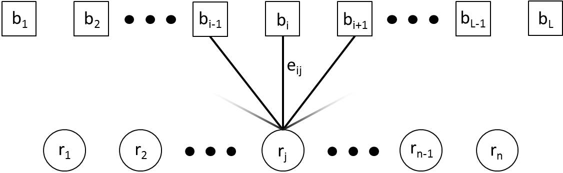
Figure 2: Illustration of the reference-guided DNA sequence assembly problem using short reads. Nodes $b_{i}$ represent bases in the target DNA sequence and $r_{j}$ represent reads. Each read node is connected to $l$ base nodes, where $l$ denotes the read length.

The bipartite graph $G(b_{1:L}\cup r_{1:n},E)$ illustrated in the figure has $L$ base nodes (representing the target genome sequence) and $n$ read nodes. Since we assume that all reads are of the same length $l$, each read node is connected to exactly $l$ base nodes. The edge $(i,j)$ in the edge set $E$ connecting $b_{i}$ and $r_{j}$ is associated with a unit vector ${\bf e}_{ij}$ indicating information about the type of base $b_{i}$ provided by the read $r_{j}$. Note that the bipartite graph described here is reminiscent of the graphical representation of the crowdsourcing problem in [21]. Motivated by the iterative learning scheme proposed there, we employ a message-passing algorithm to infer the target genome sequence using overlapping reads. Note that the previously mentioned problem of having multiple candidate locations for mapping reads can be incorporated in the proposed graphical representation and resolved using the algorithm that we describe next.

The message passing algorithms rely on the exchange of messages between neighboring nodes in the graph [24]. Our algorithm operates on real-valued base messages $\{{\bf x}_{i\rightarrow j}\}_{(i,j)\in E}$ and read messages $\{y_{j\rightarrow i}\}_{(i,j)\in E}$. A base message ${\bf x}_{i\rightarrow j}$ is a $4\times 1$ vector representing the likelihood of the base $b_{i}$ being A, C, G, or T, while a read message $y_{j\rightarrow i}$ represents the reliability of read $j$. Read messages are initialized from a random distribution, and the message update rules at iteration $k$ are given by

$${\bf x}^{(k)}_{i\rightarrow j} \leftarrow \sum_{j^{\prime}\in\partial i\backslash j}(2{\bf e}_{ij^{\prime}}-\mathds{1})y_{j^{\prime}\rightarrow i}^{(k-1)},$$ (1)

$$y_{j\rightarrow i}^{(k)} \leftarrow \frac{1}{l-1}\sum_{i^{\prime}\in\partial j\backslash i}{\bf e}_{i^{\prime}j}^{T}{\bf x}_{i^{\prime}\rightarrow j}^{(k)},$$ (2)

where $\partial i$ and $\partial j$ denote collection of the neighboring nodes of nodes $i$ and $j$, respectively, and $\mathds{1}$ is a $4\times 1$ vector containing all $1$’s. Note that $2{\bf e}_{ij^{\prime}}-\mathds{1}$ has element $1$ in the position corresponding to the nucleotide base $b_{ij^{\prime}}$ represented by ${\bf e}_{ij^{\prime}}$, and $-1$’s elsewhere. Hence a read with positive reliability value $y_{j^{\prime}\rightarrow i}$ will increase the likelihood of $b_{ij^{\prime}}$ and decrease the likelihood of other bases. Finally, the likelihood of a base being A, C, G, or T is calculated as the sum of the information provided by the reads weighted by each read’s reliability. The symbol with the highest likelihood is chosen as the estimate of the base in the corresponding position. The estimate rule for the $i^{th}$ base is

$$\hat{b}_{i}=\arg\max_{t\in\{A,C,G,T\}}{\bf x}_{i}^{\{t\}},$$ (3)

where the decision vector ${\bf x}_{i}=\sum_{j\in\partial i}(2{\bf e}_{ij}-\mathds{1})y_{j\rightarrow i}^{(k_{m})}$. Here, $k_{m}$ denotes the number of iterations performed and ${\bf x}_{i}^{\{t\}}$ denotes the likelihood corresponding to symbol $t\in\{A,C,G,T\}$ in the vector ${\bf x}_{i}=\left[{\bf x}_{i}^{\{A\}}\;{\bf x}_{i}^{\{C\}}\;{\bf x}_{i}^{\{G\}}\;{\bf x}_{i}^{\{T\}}\right]^{T}$. The procedure is formalized as Algorithm 1.

Algorithm 1 Message passing for sequence assembly

  Input: $E$, $\{{\bf e}_{ij}\}_{(i,j)\in E}$

  1 Initialize read messages:

  for all $(i,j)\in E$ do

     Initialize $y_{j\rightarrow i}^{(0)}$;

  end for

  2 Iterations:

  for $k=1\to k_{m}$ do

     for all $(i,j)\in E$ do

        Update base message:

        ${\bf x}_{i\rightarrow j}^{(k)}\leftarrow\sum_{j^{\prime}\in\partial i\backslash j}(2{\bf e}_{ij^{\prime}}-\mathds{1})y_{j^{\prime}\rightarrow i}^{(k-1)}$;

        Normalize ${\bf x}_{i\rightarrow j}^{(k)}$:

        ${\bf x}_{i\rightarrow j}^{(k)}\leftarrow\frac{{\bf x}_{i\rightarrow j}^{(k)}}{||{\bf x}_{i\rightarrow j}^{(k)}||_{2}}.$

     end for

     for all $(i,j)\in E$ do

        Update read message

        $y_{j\rightarrow i}^{(k)}\leftarrow\frac{1}{l-1}\sum_{i^{\prime}\in\partial j\backslash i}{\bf e}_{i^{\prime}j}^{T}{\bf x}_{i^{\prime}\rightarrow j}^{(k)}$;

     end for

  end for

  3 Estimation:

  for $i=1\to L$ do

     Calculate decision vector ${\bf x}_{i}=\sum_{j\in\partial i}(2{\bf e}_{ij}-\mathds{1})y_{j\rightarrow i}^{(k_{m})}$;

     Estimate the bases

     $\hat{b_{i}}=\arg\max_{t\in\{A,C,G,T\}}{\bf x}_{i}^{\{t\}}$;

  end for

Note that Algorithm 1 needs to be appropriately initialized. In our experimental studies presented in Section VI, we initialize $y_{j\rightarrow i}^{(0)}$ by drawing from both Gaussian distribution $\mathcal{N}(1,1)$ and uniform distribution $U[0,1]$. For the data sets under consideration, it turns out that different initializations lead to identical solutions. The algorithm is terminated when the reliability increment between subsequent iterations is small, i.e., $\sum|y_{j\rightarrow i}^{(k)}-y_{j\rightarrow i}^{(k-1)}|<\epsilon$. As pointed out earlier, the algorithm does not require exact knowledge of quality scores, and iteratively infers reliability of individual reads.

Since the reads originating from a single sequencing instrument have identical lengths, the degree of the read nodes in the graph is uniform. On the other hand, degree of a base node is the number of reads that cover the corresponding base, usually referred to as the sequencing coverage. Typically, coverage varies from one position to another and, consequently, degree of the base nodes varies. Note that fragmentation of multiple copies of the target sequence – a fundamental step in shotgun sequencing procedure – can be viewed as a uniform sampling from the original DNA strand. The resulting coverage is a random variable that can be described well by a Poisson distribution [26, 28].

Let $\bar{c}$ denote the average sequencing coverage. The computational complexity of the base message updating step (1), which needs to be performed in each iteration of Algorithm 1, is $\mathcal{O}(nl\bar{c})$ on average, while the complexity of the read message updating step (2) is $\mathcal{O}(nl^{2})$. Since $L\bar{c}=nl$, the complexity of the algorithm is $\mathcal{O}(k_{m}nl(l+\bar{c}))=\mathcal{O}(k_{m}L\bar{c}(l+\bar{c}))$, where $k_{m}$ denotes the number of iterations (i.e., the number of message updates). On the other hand, simple plurality voting scheme has complexity $\mathcal{O}(L\bar{c}\log\bar{c})$. Our experimental studies show that $k_{m}\leq 30$ is sufficient for the convergence of the algorithm. We tested the algorithm on a broad range of parameters (in particular, for read lengths $l\leq 100$, coverage $\bar{c}\leq 60$), and found that the runtimes are comparable to those of the state-of-the-art techniques (SAMtools and GATK) – a specific comparison of runtimes is reported in Section VI.

III Relation to standard belief propagation

As an alternative to the intuitively pleasing but basically heuristic message passing scheme proposed in Section II, we can also derive a standard belief propagation algorithm for the reference-guided sequence assembly. To this end, we seek the sequence $\hat{b}_{1:L}$ that maximizes the joint probability $P(\hat{b}_{1:L},p_{1:n})$, where $p_{1:n}$ denotes confidences of the aligned read data and $p_{j}\in[0,1]$. This maximization can be formalized as

$$\max_{\hat{b}_{1:L},p_{1:n}}\prod_{j=1}^{n}\mathcal{D}(p_{j})\prod_{(i,j)\in E}\left\{p_{j}\delta(\hat{b}_{i}={\bf e}_{ij})+\bar{p}_{j}\delta(\hat{b}_{i}\neq{\bf e}_{ij})\right\},$$ (4)

where $\mathcal{D}(p_{i})$ denotes the prior distribution on $p_{i}$ and $\bar{p}_{j}=1-p_{j}$. $\delta(\cdot)$ denotes an indicator function taking value $1$ if its argument is true and is $0$ otherwise. The joint optimization is computationally challenging and thus often practically not feasible. As an alternative, belief propagation provides an approximate solution to (4) by computing the marginal distributions of the optimization variables and selecting their most likely values according to the computed distributions. A thorough review of theoretical and practical aspects of the belief propagation method can be found in [23]. For the graphical model proposed in Section II, we define two messages to facilitate belief propagation: $\tilde{x}_{i\rightarrow j}$ and $\tilde{y}_{j\rightarrow i}$. The former is the belief on $\hat{b}_{i}$ and essentially represents a distribution over the four possible nucleotide bases $\{{\bf e}_{A},{\bf e}_{C},{\bf e}_{G},{\bf e}_{T}\}$. The latter is a probability of $p_{j}$ on $[0,1]$. In the $k^{th}$ iteration of the belief propagation algorithm, message update rules are given by (see, e.g., [23] and the references therein)

$$\tilde{y}_{j\rightarrow i}^{(k)}(p_{j}) \propto \mathcal{D}(p_{j})\prod_{i^{\prime}\in\partial j\setminus i}\sum_{m=A,C,G,T}\Big{\{}p_{j}\delta({\bf e}_{i^{\prime}j}={\bf e}_{m})$$ (5)

$$+\bar{p}_{j}\delta({\bf e}_{i^{\prime}j}\neq{\bf e}_{m})\Big{\}}\tilde{x}_{i^{\prime}\rightarrow j}^{(k)}({\bf e}_{m}),$$

$$\tilde{x}_{i\rightarrow j}^{(k+1)}(\hat{b}_{i}) \propto \prod_{j^{\prime}\in\partial i\setminus j}\int\Big{(}\tilde{y}_{j^{\prime}\rightarrow i}^{(k)}(p_{j^{\prime}})(p_{j^{\prime}}\delta(\hat{b}_{i}={\bf e}_{ij^{\prime}})$$ (6)

$$+\bar{p}_{j^{\prime}}\delta(\hat{b}_{i}\neq{\bf e}_{ij^{\prime}})\Big{)}dp_{j^{\prime}}.$$

After the completion of the iterative procedure, the bases $b_{i}$ in the target genome are estimated by first computing the beliefs $\tilde{x}_{i}(\hat{b}_{i})\propto$

$$\prod_{j^{\prime}\in\partial i}\int\Big{(}\tilde{y}_{j^{\prime}\rightarrow i}^{(k)}(p_{j^{\prime}})(p_{j^{\prime}}\delta(\hat{b}_{i}={\bf e}_{ij^{\prime}})+\bar{p}_{j^{\prime}}\delta(\hat{b}_{i}\neq{\bf e}_{ij^{\prime}}))\Big{)}dp_{j^{\prime}},$$ (7)

where $\hat{b}_{i}\in\{{\bf e}_{A},{\bf e}_{C},{\bf e}_{G},{\bf e}_{T}\}$, and then choosing the base with the highest $\tilde{x}_{i}$ value. Note that, by exploiting the symmetry of the expression (4), we can write

$$\tilde{x}_{i\rightarrow j}^{(k+1)}(\hat{b}_{i}\neq{\bf e}_{m}) \propto \prod_{j^{\prime}\in\partial i\setminus j}\int\Big{(}\tilde{y}_{j^{\prime}\rightarrow i}^{(k)}(p_{j^{\prime}})(p_{j^{\prime}}\delta({\bf e}_{ij^{\prime}}\neq{\bf e}_{m})$$

$$+\bar{p}_{j^{\prime}}\delta({\bf e}_{ij^{\prime}}={\bf e}_{m})\Big{)}dp_{j^{\prime}}.$$

For the brevity of notation, we denote $\tilde{x}_{i\rightarrow j}^{(k)}({\bf e}_{m})=\tilde{x}_{i\rightarrow j}^{(k)}(\hat{b}_{i}={\bf e}_{m})$. Assuming that the prior distribution on $p_{j}$, $\mathcal{D}(p_{j})$, is Beta(0,0) (which is essentially as same as the Bernoulli(1/2) distribution), the read confidence is a binary variable,

$$p_{j}=\left\{\begin{array}[]{cc}0,\mbox{ w.p. }1/2,\\ 1,\mbox{ w.p. }1/2.\end{array}\right.$$

Define a log-likelihood ratio

$$y_{j\rightarrow i}^{k}=\log\Big{(}\frac{\tilde{y}_{j\rightarrow i}^{(k)}(1)}{\tilde{y}_{j\rightarrow i}^{(k)}(0)}\Big{)}.$$ (8)

After substituting (5) in (8), we obtain

$$y_{j\rightarrow i}^{(k)} = \sum_{i^{\prime}\in\partial j\setminus i}\log\frac{\tilde{x}_{i^{\prime}\rightarrow j}^{(k)}({\bf e}_{i^{\prime}j})}{\sum_{{\bf e}_{m}\neq{\bf e}_{i^{\prime}j}}\tilde{x}_{i^{\prime}\rightarrow j}^{(k)}({\bf e}_{m})}$$ (9)

$$= \sum_{i^{\prime}\in\partial j\setminus i}\log\frac{\tilde{x}_{i^{\prime}\rightarrow j}^{(k)}({\bf e}_{i^{\prime}j})}{\tilde{x}_{i^{\prime}\rightarrow j}^{(k)}(\hat{b}_{i^{\prime}}\neq{\bf e}_{i^{\prime}j})}.$$

Define a $4\times 1$ vector message ${\bf x}_{i\rightarrow j}^{(k)}$ as

$${\bf x}_{i\rightarrow j}^{(k)}=\left[{\bf x}_{i\rightarrow j}^{(k)}(1)\;\;\;{\bf x}_{i\rightarrow j}^{(k)}(2)\;\;\;{\bf x}_{i\rightarrow j}^{(k)}(3)\;\;\;{\bf x}_{i\rightarrow j}^{(k)}(4)\right]^{T},$$

where

$$\begin{array}[]{lr}{\bf x}_{i\rightarrow j}^{(k)}(1)=\log\frac{\tilde{x}_{i\rightarrow j}^{(k)}({\bf e}_{A})}{\tilde{x}_{i\rightarrow j}^{(k)}(\hat{b}_{i}\neq{\bf e}_{A})},\;{\bf x}_{i\rightarrow j}^{(k)}(2)=\log\frac{\tilde{x}_{i\rightarrow j}^{(k)}({\bf e}_{C})}{\tilde{x}_{i\rightarrow j}^{(k)}(\hat{b}_{i}\neq{\bf e}_{C})},\\ {\bf x}_{i\rightarrow j}^{(k)}(3)=\log\frac{\tilde{x}_{i\rightarrow j}^{(k)}({\bf e}_{G})}{\tilde{x}_{i^{\prime}\rightarrow j}^{(k)}(\hat{b}_{i^{\prime}}\neq{\bf e}_{G})},\;{\bf x}_{i\rightarrow j}^{(k)}(4)=\log\frac{\tilde{x}_{i\rightarrow j}^{(k)}({\bf e}_{T})}{\tilde{x}_{i^{\prime}\rightarrow j}^{(k)}(\hat{b}_{i^{\prime}}\neq{\bf e}_{T})}.\end{array}$$

It is straightforward to write

$$y_{j\rightarrow i}^{(k)}=\sum_{i^{\prime}\in\partial j\setminus i}{\bf e}_{i^{\prime}j}{\bf x}_{i^{\prime}\rightarrow j}^{(k)}.$$ (10)

A closer examination of the first element of ${\bf x}_{i\rightarrow j}^{(k)}$, ${\bf x}_{i\rightarrow j}^{(k)}(1)$, leads to simplification shown in (13), where we implicitly used the assumption that $p_{j}$ is binary.

$${\bf x}_{i\rightarrow j}^{(k)}(1) = \log\frac{x_{i\rightarrow j}^{(k)}({\bf e}_{A})}{x_{i\rightarrow j}^{(k)}(\hat{b}_{i}\neq{\bf e}_{A})}=\sum_{j^{\prime}\in\partial i\setminus j}\log\frac{\int\left(\tilde{y}_{j^{\prime}\rightarrow i}^{(k-1)}(p_{j^{\prime}})(p_{j^{\prime}}\delta({\bf e}_{ij^{\prime}}={\bf e}_{A})+\bar{p}_{j^{\prime}}\delta({\bf e}_{ij^{\prime}}\neq{\bf e}_{A})\right)dp_{j^{\prime}}}{\int\left(\tilde{y}_{j^{\prime}\rightarrow i}^{(k-1)}(p_{j^{\prime}})(p_{j^{\prime}}\delta({\bf e}_{ij^{\prime}}\neq{\bf e}_{A})+\bar{p}_{j^{\prime}}\delta({\bf e}_{ij^{\prime}}={\bf e}_{A})\right)dp_{j^{\prime}}}$$ (13)

$$= \left\{\begin{array}[]{ll}\log\frac{\tilde{y}_{j^{\prime}\rightarrow i}^{(k-1)}(1)}{\tilde{y}_{j^{\prime}\rightarrow i}^{(k)}(0)}=y_{j^{\prime}\rightarrow i}^{(k-1)}&\mathrm{if}\;{\bf e}_{ij^{\prime}}={\bf e}_{A}\\ -\log\frac{\tilde{y}_{j^{\prime}\rightarrow i}^{(k-1)}(1)}{\tilde{y}_{j^{\prime}\rightarrow i}^{(k)}(0)}=-y_{j^{\prime}\rightarrow i}^{(k-1)}&\mathrm{if}\;{\bf e}_{ij^{\prime}}\neq{\bf e}_{A}\end{array}\right.$$

 

We can obtain similar expressions to (13) for other components of ${\bf x}_{i\rightarrow j}^{(k)}$. As a result, the updating rule for ${\bf x}_{i\rightarrow j}^{(k)}$ simplifies,

$${\bf x}_{i\rightarrow j}^{(k)}=\sum_{j^{\prime}\in\partial i\setminus j}(2{\bf e}_{ij^{\prime}}-\mathds{1})y_{j^{\prime}\rightarrow i}^{(k-1)},$$ (14)

where the vector $2{\bf e}_{ij^{\prime}}-\mathds{1}$ has element $1$ in the position corresponding to the nucleotide base $b_{ij^{\prime}}$ represented by ${\bf e}_{ij^{\prime}}$, and $-1$’s elsewhere. Therefore, the belief propagation update rule (14) is identical to the update rule (1) of our message passing algorithm presented in Section II. Moreover, update rule (10) is identical (up to the scaling factor) to the message update rule (2). Therefore, message passing scheme proposed in Section II can be interpreted as the belief propagation under a specific prior on the confidence of the aligned data $p_{j}$ – in particular, $p_{j}$ should come from a Beta(0,0) distribution, i.e., be treated as a binary variable.

IV Binary representation, message passing, and power iteration algorithm

So far, we discussed reference-guided assembly schemes that rely on a representation of the nucleotide basis with $4$-dimensional vectors $\{{\bf e}_{A},{\bf e}_{C},{\bf e}_{G},{\bf e}_{T}\}$. As an alternative, in this section we rely on a binary representation of nucleotides to formulate a message passing scheme and discuss the provably convergent power iteration algorithm for finding the target genome sequence. The power iteration scheme finds the desired sequence by computing the leading singular vectors of an appropriately defined data matrix.

The four-letter alphabet $\{A,C,G,T\}$ in DNA sequencing data can be represented using binary symbols, e.g., $\{+1,-1\}$. In particular, we encode the nucleotide basis as $A=\{-1,-1\}$, $C=\{-1,+1\}$, $G=\{+1,-1\}$, and $T=\{+1,+1\}$, and represent reads as binary sequences comprising $\{\pm 1\}$. Similar to how we built a model utilizing $4$-dimensional vectors $\{{\bf e}_{A},{\bf e}_{C},{\bf e}_{G},{\bf e}_{T}\}$ in Section II, we define a bipartite graph where each base $b_{i}$ is represented by two binary nodes $\tilde{b}_{2i-1}$ and $\tilde{b}_{2i}$. Using the output of an alignment algorithm, each read node of the bipartite graph is connected to $2l$ binary base nodes in the node set $\tilde{b}_{1:2L}$, where $l$ denotes read length and $L$ is the length of the target sequence. For convenience, let us denote the resulting graph by $G(\tilde{b}_{1:2L}\cup r_{1:n},\tilde{E})$. The edge $(k,j)$ in $\tilde{E}$ connecting $\tilde{b}_{k}$ and $r_{j}$ is assigned a variable $e_{kj}\in\{\pm 1\}$, the binary representation of $\tilde{b}_{k}$ provided by read $r_{j}$. Given such a graphical representation, we can apply a binary message passing algorithm as in [21]. In particular, the read and base messages are scalars and the update equations are given by

$$x^{(k)}_{i\rightarrow j} \leftarrow \sum_{j^{\prime}\in\partial i\backslash j}e_{ij^{\prime}}y_{j^{\prime}\rightarrow i}^{(k-1)},$$ (15)

$$y_{j\rightarrow i}^{(k)} \leftarrow \sum_{i^{\prime}\in\partial j\backslash i}e_{i^{\prime}j}^{T}x_{i^{\prime}\rightarrow j}^{(k)}.$$ (16)

After the iterative procedure reaches a stopping criterion, the binary string representing unknown target DNA sequence is obtained as the weighted average

$$\tilde{b}_{i}=\mathrm{sign}(\sum_{j^{\prime}\in\partial i\backslash j}e_{ij^{\prime}}y_{j^{\prime}\rightarrow i}).$$ (17)

The above algorithm is known to converge to the optimal solution when the bi-partite graph is regular [22]. In our application, however, the graph is not regular since the sequencing coverage varies. Nevertheless, we find that the binary message-passing algorithm performs very well in both simulations and on experimental data, as we demonstrate in Section VI. The binary message passing algorithm is also closely related to the so-called power iteration scheme for computing the leading singular vector of an appropriately defined data matrix. We next examine the power iteration algorithm and argue its convergence.

With the adopted binary encoding of nucleotides, we can represent sequencing reads by a sparse $n\times 2L$ matrix $D$. The $2L$ columns of $D$ correspond to the $L$ positions in the target sequence whereas the $j^{th}$ row of $D$ comprises binary data representing read $r_{j}$. In each row, only $2l$ entries are non-zero (representing an $l$-long read) while the remaining ones are filled with zeros. Therefore, matrix $D$ has entries $D_{ij}\in\{0,+1,-1\}$. Since the percentage of nonzero entries of $D$ is $\frac{2l}{L}$ and $L\gg l$, $D$ is a sparse matrix. It is easy to show (see, e.g., [22]) that if each row of $D$ has the same number of nonzero entries, and the same holds for each column, the left singular vector corresponding to the largest singular value of $D$ is a reliable estimate of the target genome sequence when the measurement noise (i.e., read error rate) is low. Here is an illustration. Let $s$ denote the $2L\times 1$ binary vector with alphabet $\{-1,+1\}$ representing the true sequence of length $L$, and let the number of nonzero entries in each columns of $D$ be $c$. Consider the case where the reads are error-free and $s$ is a $2L\times 1$ all one vector $\mathds{1}_{2L}$. Since $DD^{T}\mathds{1}_{2L}=2Lc\mathds{1}_{2L}$, then $s$ is an eigenvector of $DD^{T}$. Here $D$ is a non-negative matrix with entries $0$s and $1$s and thus, by Perron-Frobenius theorem, $\mathds{1}_{2L}$ is a left singular vector corresponding to $D$’s largest singular value. In the general case where $s$ consists of both $1$ and $-1$, we can represent $s=S\mathds{1}_{2L}$ where $S$ is a $2L\times 2L$ diagonal matrix with $\mathrm{diag}(S)=s$. In this case, it is straightforward to generalize the above analysis and show that $s$ remains to be proportional to the leading singular vector of the matrix $D$.

Performing singular value decomposition is roughly cubic in the dimension of $D$ and, for our problem dimensions, clearly infeasible. Fortunately, we only need to find ${\bf u}$, the leading singular vector of $D$, and then estimate the target sequence $s$ as $\mathrm{sign}({\bf u})$. This can be done in a computationally efficient way using the power iteration technique due to sparsity of $D$. In particular, the power iteration procedure entails computing

$${\bf x}^{(k)}=D{\bf y}^{(k-1)},\;\;\;{\bf y}^{(k)}=D^{T}{\bf x}^{(k)}.$$ (18)

To demonstrate convergence of the power iteration scheme (18), let us denote the singular values of $D$ as $\sigma_{i}(D)$, where $\sigma_{1}(D)\geq\sigma_{2}(D)\geq...\geq 0$. With a random initialization ${\bf y}^{(0)}$, power iterations will converge to the singular vector ${\bf u}$ if the inequality $\sigma_{1}(D)>\sigma_{2}(D)$ holds strictly. The speed of the convergence of power iterations depends on the ratio $\sigma_{2}(D)/\sigma_{1}(D)$. This can be easily shown by an analysis of the consecutive projections of the iteratively updated vectors ${\bf x}^{(k)}$ onto the singular vector ${\bf u}$. In particular, the projection of ${\bf x}^{(k)}$ onto ${\bf u}$ is $({\bf u}^{T}{\bf x}^{(k)}){\bf u}$. A closer look into the singular value decomposition shows that ${\bf u}^{T}{\bf x}^{(k)}{\bf u}=(\sigma_{1}(D))^{2}{\bf u}^{T}{\bf x}^{(k-1)}{\bf u}$ and $({\bf x}^{(k)}-{\bf u}^{T}{\bf x}^{(k)}{\bf u})\leq(\sigma_{2}(D))^{2}({\bf x}^{(k-1)}-{\bf u}^{T}{\bf x}^{(k-1)}{\bf u})$. Therefore,

$$\frac{||{\bf x}^{(k)}-{\bf u}^{T}{\bf x}^{(k)}{\bf u}||}{||{\bf u}^{T}{\bf x}^{(k)}{\bf u}||} \leq \left(\frac{\sigma_{2}(D)}{\sigma_{1}(D)}\right)^{2}\frac{||{\bf x}^{(k-1)}-{\bf u}^{T}{\bf x}^{(k-1)}{\bf u}||}{||{\bf u}^{T}{\bf x}^{(k-1)}{\bf u}||}$$

$$\leq \left(\frac{\sigma_{2}(D)}{\sigma_{1}(D)}\right)^{2k}\frac{||{\bf x}^{(0)}-{\bf u}^{T}{\bf x}^{(0)}{\bf u}||}{||{\bf u}^{T}{\bf x}^{(0)}{\bf u}||}.$$

Clearly, power iterations will converge with any initialization if $\sigma_{1}(D)>\sigma_{2}(D)$, and the speed of convergence depends on the ratio of $\sigma_{1}(D)$ and $\sigma_{2}(D)$ – the larger the ratio, the faster the convergence. On the other hand, from (18) it directly follows that the update equations for the entries of ${\bf x}^{(k)}$ and ${\bf y}^{(k)}$ can be written as

$$x_{i}^{(k)}=\sum_{j\in\partial i}D_{ij}y_{j}^{(k-1)},\;\;\;y_{j}^{(k)}=\sum_{i\in\partial j}D_{ij}x_{i}^{(k)}.$$ (19)

Note that the power iterations (19) differ from the message update rules (15) and (16) in only one term. As our results in Section VI show, accuracy of message passing and power iterations is essentially identical, while the former converges in significantly fewer iterations than the latter. Moreover, both message-passing schemes – the one based on the representation of basis via $4$-dimensional vectors $\{{\bf e}_{A},{\bf e}_{C},{\bf e}_{G},{\bf e}_{T}\}$ as well as the one relying on the binary representation of nucleotides – converge after approximately the same number of iterations.

V Benchmarking performance of the proposed assembly schemes

To assess and benchmark performance of the proposed iterative learning schemes, in this section we analyze the probability of error of a genie-aided maximum a posteriori (MAP) estimator of the bases in the target genome sequence. In this problem, ”genie-aided” is referring to an idealized scenario where short reads are mapped to the reference genome with no errors, i.e., there are no misplacements of the reads along the reference sequence and the MAP estimator knows exact probabilities of mis-calling the bases in the short reads (i.e., has exact quality score information). Recall that neither our message-passing schemes nor the power iteration algorithm make such practically unrealistic assumptions and, in fact, do not require prior knowledge of quality scores.

V-A Genie-aided MAP estimator

Let $b_{k}$ denote the $k^{th}$ base in the target sequence, and let $y^{(i)}_{k}$ denote the signal generated by the sequencing platform as it examines $b_{k}$, $i=1,2,\ldots,c_{k}$, where $c_{k}$ stands for the total number of reads covering $b_{k}$. Assume that the probability of erroneously calling $b_{k}$ in the $i^{th}$ read is $p^{(i)}_{k}$. Given the base calls of the reads covering $b_{k}$, $y^{(i)}_{k}$, the MAP estimate $\hat{b}_{k}$ is readily found as

$$\hat{b}_{k} = \arg\max_{x}\prod_{i=1}^{c_{k}}P(y^{(i)}_{k},b_{k}=x)$$

$$= \arg\max_{x}\prod_{i=1}^{c_{k}}P(y^{(i)}_{k}|b_{k}=x)P(b_{k}=x)$$

$$= \arg\max_{x}\prod_{i=1}^{c_{k}}(1-p^{(i)}_{k})^{\delta(y^{(i)}_{k}=x)}(p^{(i)}_{k})^{(1-\delta(y^{(i)}_{k}=x))}P(b_{k}=x)$$

$$= \arg\max_{x}\sum_{i=1}^{c_{k}}\Big{[}\delta(y^{(i)}_{k}=x)\log(1-p^{(i)}_{k})$$

$$+ (1-\delta(y^{(i)}_{k}=x))\log(p^{(i)}_{k})\Big{]}+\log(P(b_{k}=x))$$

$$= \arg\max_{x}\sum_{i=1}^{c_{k}}\delta(y^{(i)}_{k}=x)w^{(i)}_{k}+\log(p^{(i)}_{k})$$

$$+ \log(P(b_{k}=x)),$$

where we introduced $w^{(i)}_{k}=\log\Big{(}\frac{1-p^{(i)}_{k}}{p^{(i)}_{k}}\Big{)}$. Therefore, the MAP estimate $\hat{b}_{k}$ formed by combining the information provided by $c_{k}$ reads covering $b_{k}$ is given by

$$\hat{b}_{k}=\arg\max_{x}\sum_{i=1}^{c_{k}}w^{(i)}_{k}\delta(y^{(i)}_{k}=x)+\log(P(b_{k}=x)).$$ (20)

In the absence of prior information $P(b_{k}=x)$, the MAP estimation of $b_{k}$ in (20) is identical to the so-called weighted plurality voting [25]. Note that if $p^{(i)}_{k}=p$ for all $i$ and $k$, (20) becomes the well-known plurality voting scheme.

Intuitively, we expect that the performance of the MAP decision scheme improves as we increase the coverage $c_{k}$. Note that the above expressions are predicated on the assumption of error-free read mapping.

V-B Performance of the genie-aided MAP estimator

For notational convenience, let us write the expression for the estimate in (20) as

$$\hat{b}_{k}=\arg\max_{x}W_{k}(x),$$ (21)

where $W_{k}(x)=\displaystyle\sum_{i:y^{(i)}_{k}=x}w^{(i)}_{k}+\log(P(b_{k}=x))$. The probability of error is defined as $P(\hat{b}_{k}\neq b_{k})=1-P(\hat{b}_{k}=b_{k})$.

To characterize the probability of error of the MAP decision scheme, we rely on the so-called universal generating functions often used in reliability analysis of multi-state systems [27]. Consider $n$ independent discrete random variables $X_{1},\ldots,X_{n}$ with probability mass functions (pmf) represented by vectors $(\bm{x}_{i},\bm{p}_{i})$ (e.g., $P(X_{i}=x_{ij})=p_{ij}$). In order to evaluate the pmf of an arbitrary function $f(X_{1},\ldots,X_{N})$, one has to find the vector $\bm{y}$ of all the possible values of $f(\cdot)$ and the vector $\bm{q}$ of the corresponding probabilities. The total number of possible combinations $(X_{1},\ldots,X_{N})$ is $K=\prod_{i=1}^{n}(k_{i}+1)$, where $(k_{i}+1)$ is the number of different realizations of $X_{i}$. Since the variables are independent, the probability of each unique combination is equal to the product of the probabilities of the realizations of arguments composing this combination. The probability of the $j^{th}$ combination of the realizations of the variables is $q_{j}=\prod_{i=1}^{n}p_{ij}$ and the corresponding value of the function is $f_{j}=f(x_{1j_{1}},\ldots,x_{nj_{n}})$. If different combinations produce the same value of the function, then the probability that $f(\cdot)$ takes that value is equal to the sum of probabilities of the combinations resulting in it. As an illustration, let $A_{h}$ denote the set of combinations resulting in the particular function value $f_{h}$. If the total number of different values that the function of random variables $f(X_{1},\ldots,X_{n})$ may assume is $H$, then its probability mass function is completely specified with a pair of vectors $(\bm{y},\bm{q})$ defined as

$$\bm{y} = (f_{h}:1\leq h\leq H),$$

$$\bm{q} = \Big{(}\sum_{(x_{1j_{1}},\ldots,x_{nj_{n}})\in A_{h}}\prod_{i=1}^{n}p_{ij_{i}}:1\leq h\leq H\Big{)}.$$

A compact representation of the probability mass function of a random variable $X_{i}$, $(x_{i0},x_{i1},\ldots,x_{ik_{i}},p_{i0},p_{i1},\ldots,p_{ik_{i}})$, is given by a z-transform that takes the polynomial form

$$u_{i}(z)=\sum_{j=0}^{k_{i}}p_{ij}z^{x_{ij}}.$$ (22)

Such a representation is convenient since, to find the probability that $X_{i}\in\Phi$, one can use operator $\delta$ defined as

$$Pr(X_{i}\in\Phi)=\delta(u_{i}(z),\Phi)=\sum_{j:x_{ij}\in\Phi}p_{ij}.$$ (23)

Moreover, the z-transform representation enables straightforward calculation of the probability mass function of an arbitrary function $f$ of $n$ independent random variables. This can be facilitated via the composition operator ${\otimes}_{f}$ applied to z-transform representations of the probability mass functions of the variables,

$${\otimes}_{f}\Big{(}\sum_{j_{i}=0}^{k_{i}}p_{ij_{i}}z^{x_{ij_{i}}}\Big{)}=\sum_{j_{1}=0}^{k_{1}}\ldots\sum_{j_{1}=0}^{k_{n}}\Big{(}\prod_{i=0}^{n}p_{ij_{i}}z^{f(x_{1j_{1}},\ldots,x_{nj_{n}})}\Big{)}.$$ (24)

The technique for finding probability mass functions that relies on the z-transform and composition operators ${\otimes}_{f}$ is referred to as the universal z-transform or the universal (moment) generating function (UGF) technique. In the context of this technique, the z-transform of a random variable for which the operator ${\otimes}_{f}$ is defined is often referred to as its U-function. For additional background on this subject, we refer an interested reader to [27]. Here, we rely on this technique to characterize the probability of error of the genie-aided sequence assembly scheme.

Consider the U-function (similar to (22)) defined for each read position

$$U_{i}(z) = \sum_{m=1}^{4}s^{i}_{m}z^{v^{i}_{m}}$$ (25)

$$= r^{(i)}_{x_{1}}z^{[w_{i}(x_{1})\hskip 1.42262pt0\hskip 1.42262pt0\hskip 1.42262pt0]}+r^{(i)}_{x_{2}}z^{[0\hskip 1.42262ptw_{i}(x_{2})\hskip 1.42262pt0\hskip 1.42262pt0]}$$

$$+ r^{(i)}_{x_{3}}z^{[0\hskip 1.42262pt0\hskip 1.42262ptw_{i}(x_{3})\hskip 1.42262pt0]}+r^{(i)}_{x_{3}}z^{[0\hskip 1.42262pt0\hskip 1.42262pt0\hskip 1.42262ptw_{i}(x_{4})]},$$

where $r^{i}_{x_{j}}$ denotes the probability that the symbol from read $i$ is $x_{j}$, and $w_{i}(x_{j})$ is the weight associated with the information provided by read $i$ (essentially given by the quality scores, which the genie-aided scheme assumes to be perfectly known). To obtain a U-function of the decision for two positions having respective U-functions $U_{1}(z)$ and $U_{2}(z)$, the following composition operator can be used,

$$U_{1,2}(z) = \Omega\Big{(}U_{1}(z),U_{2}(z)\Big{)}$$ (26)

$$= \Omega\Big{(}\sum_{m=1}^{4}s^{1}_{m}z^{v^{1}_{m}},\sum_{m=1}^{4}s^{2}_{m}z^{v^{2}_{m}}\Big{)}$$

$$= \sum_{m=1}^{4}\sum_{n=1}^{4}s^{1}_{m}s^{2}_{n}z^{v^{1}_{m}+v^{2}_{m}}$$

$$= \sum_{m}s^{\{1,2\}}_{m}z^{v^{\{1,2\}}_{m}}.$$

Note that some combinations of $v^{1}_{m}$ and $v^{2}_{m}$ may lead to the same $v^{1}_{m}+v^{2}_{m}$ and hence there may be multiple terms in (26) that involve $z^{v^{1}_{m}+v^{2}_{m}}$. If so, in the last step in (26), such terms are summed up to obtain $s^{\{1,2\}}_{m}$ which is referred to as the read output distribution of reads 1 and 2. The support set of $s^{\{1,2\}}_{m}$ is at most $4^{2}=16$, but may be smaller due to aforementioned grouping of the terms that involve identical vectors.

The above procedure leads to a representation of the probability of error of arriving at the decision for a particular sequence position by combining information provided by two reads. Given an arbitrary subset of reads $\lambda$ (e.g., so far we discussed $\lambda=\{1,2\}$), it is straightforward to obtain the U-function for an extended subset $\lambda\cup{j}$ with an arbitrary $j\notin\lambda$ as

$$U_{\lambda\cup j}(z) = \Omega\Big{(}U_{\lambda}(z),U_{j}(z)\Big{)}=\sum_{m}s^{\lambda\cup j}_{m}z^{v^{\lambda\cup j}_{m}}.$$ (27)

We can further simplify and arrive at more explicit expressions in the following way. Consider the U-function of an arbitrary weighted voting classifier (WVC) over a subset of reads $\lambda$,

$$U_{\lambda}(z)=\sum_{m}s^{\lambda}_{m}z^{v^{\lambda}_{m}}.$$ (28)

Let $W_{\Lambda}=\sum_{j\in\Lambda}w_{j}$ be the total weight of all the votes belonging to the WVC, and let the total weight of the subsystem $\lambda$ be given by $W_{\lambda}$. The weight not belonging to $\lambda$ can be expressed as

$$\sigma=\sum_{j\neq\lambda}w_{j}=W_{\Lambda}-W_{\lambda}.$$ (29)

Note that if $W$ is the largest element of the vector $v^{\lambda}_{m}$ and $v^{\lambda}_{m}(W)-v^{\lambda}_{m}(i)>\sigma$, then any element $v^{\lambda}_{m}(i)\neq W$ can be set to zero since this does not affect the probability of reliability even if all of the remaining votes are given to $i$. Similarly, vectors satisfying $v^{\lambda}_{m}(W)-v^{\lambda}_{m}(1)>\sigma$, $W\neq 1$ can be removed from further consideration for the same reason. After these simplifications, the probability of correctly identifying the base is given by

$$P(\hat{b}_{k}=b_{k})=r_{k}=\delta(U_{\Lambda},\hat{b}_{k})=\sum_{\hat{b}_{k}(V^{\Lambda}_{m})=b_{k}}s^{\Lambda}_{m},$$ (30)

where $\Lambda=\{1,2,\ldots,c_{k}\}$. The steps for computing the error probability of decision for a given set of read positions are summarized below.

Algorithm 2 Computation of $P(\hat{b}_{k}=b)$

  1. For each observations $y^{(i)}_{k},1\leq i\leq c_{k}$, define $U_{i}(Z)$ according to (25).

  2. Determine U-functions $U_{\Lambda}(z)$ for entire reads (in an arbitrary order) by applying (26) and (27) and collecting identical terms in the intermediate U-function.

  3. Simplify expressions (zeroing or removing as discussed).

  4. Apply $\delta$-operator (30) to obtain the probability of correct classification $r_{k}$ and the probability of error as $1-r_{k}$.

Having computed the probability of error $P(\hat{b}_{k}\neq b_{k})$ for a fixed coverage $c_{k}$ (where the MAP estimator forms $\hat{b}_{k}$ by combining information from $c_{k}$ reads that cover the $k^{th}$ base), we can readily evaluate the probability of error for a random coverage. In particular, the average assembly error probability $P_{error}$ can be found by evaluating

$$P_{error}=\sum_{c_{k}}P(c=c_{k})P(\overline{err}_{c}|c=c_{k}),$$ (31)

where $\overline{err}_{c_{k}}$ denotes the error averaged over different read positions given a fixed $c_{k}$. The probability distribution of $c$ is often assumed to be Poisson [26], [28] with some parameter $\lambda$. Assuming a non-zero coverage, the mean coverage is given by $\bar{c}=\frac{\lambda}{1-\exp(-\lambda)}$ [28]. With bases not covered by any reads we associate the probability of error of $\frac{3}{4}$. Thus we can write the average error probability (conditioned on the coverage depth being at least $1$) as

$$P_{error}=\frac{1}{1-\exp(-\lambda)}\sum_{c_{k}=1}^{\infty}\frac{\lambda^{c}\exp^{-\lambda}}{c!}P(\overline{err}_{c}|c=c_{k}).$$ (32)

Note that the fraction of bases not covered by any read is given by $\exp(-\lambda)$ and thus the overall probability of error is given by $P_{total}=\frac{3}{4}\exp(-\lambda)+P_{error}$. For distributions other than Poisson, e.g., empirical distributions inferred from data, one can still apply the above approach to perform a semi-analytical evaluation of $P_{error}$.

VI Experimental Results

In this section we present performance studies using both simulations and experimental data sets. First, using realistic synthetic data, we compare the performance of the message passing algorithm from Section II (Algorithm 1), the binary message passing algorithm and the power iteration algorithm. Moreover, we examine the convergence properties of all these schemes and benchmark their accuracy by comparing it with the genie-aided MAP estimation employed in the idealistic scenario where the exact error probabilities of the reads are known. Then we proceed by testing the algorithms on the experimental data we obtained by sequencing E. Coli and N. Meningitides using the Illumina’s HiSeq sequencing instrument that provides $100$-bp long reads. In particular, we compare the performance of our developed reference-guided sequence assembly algorithms with the commonly used sequencing data analysis tools including GATK and SAMtools.

VI-A Simulation data

We simulated reference-guided sequence assembly of the genome of a strain of Neisseria Meningitidis. The reference sequence is obtained from GenBank (http://www.ncbi.nlm.nih.gov/nuccore) database and is $L=2,184,406$ bases long. The reference is used to generate target sequences having $1\%$ variation rate. We then uniformly select starting positions along the sequence and simulate short reads of length $l=76$ (mimicking Illumina’s Genome Analyzer II platform). Sequencing errors in these reads are simulated according to the position-dependent base calling error profile typical of this particular sequencing platform [6]. The average error rate of the base calling procedure is $0.015$ (averaged over all reads and bases in the reads). To construct the bipartite graphical model, we map the reads to the reference sequence using an alignment algorithm based on the Burrows-Wheeler transform [16] and thus establish connections (i.e., edges) between the read nodes and their aligned base nodes. The read nodes with multiple candidate mapping positions are replicated (where each replica may be assigned different confidence score), and each replica is connected to its corresponding set of base nodes. The bipartite graph with binary base nodes introduced in Section IV is constructed in the same way. We apply both the message passing algorithms from Section II and Section IV to infer the target sequence (note that since the algorithms are randomly initialized, the stopping points and hence the resulting assembled sequences may be different). We also form the binary data matrix representing all the short read data and employ the power iteration method to infer the target genome sequence. While the analysis in Section IV gives a guarantee of convergence of the power iteration algorithm, we found that its convergence is usually faster than the theoretical bound. We set the stopping criterion for all these iterative learning methods as $\sum|y_{j\rightarrow i}^{(k)}-y_{j\rightarrow i}^{(k-1)}|<\epsilon=0.01L$. It turns out that both message passing algorithms need $\sim 30$ iterations to converge, while the power iterations converge in $\sim 50$ iterations. We initialize all these algorithm by generating $y_{j\rightarrow i}^{(0)}$ from Gaussian distribution $\mathcal{N}(1,1)$ and uniform distribution $U(0,1)$ – our extensive simulation studies indicate that different initializations lead to the same error rate of the considered iterative schemes.

For a comparison, we also consider the plurality voting based decision scheme often used in practice (see, e.g., [26]). Here, multiple calls for a base in any given position along the target sequence are consolidated by performing plurality voting. Notice that, in both message passing and plurality voting, we assume the error profiles of the reads (i.e., base calling error rates) are unknown. Plurality voting assumes all reads has equal reliability while message passing scheme iteratively infers the reliability of each read. We also consider probability of error of the MAP decision scheme in Section III which assumes perfect knowledge of the positions of reads along the target sequence and exact information about position-dependent base calling errors (both assumptions are unrealistic in practice). The error rates of these algorithms are shown in Fig. 3 for various sequencing coverages (horizontal axis shows the average coverage). As can be seen from Fig. 3, the message-passing scheme and the power iteration algorithm outperform plurality voting. The binary message passing algorithm has almost identical accuracy as power iterations, while being slightly worse than Algorithm 1. Moreover, we see that the error rates of message passing are close to the genie-aided MAP decision scheme.

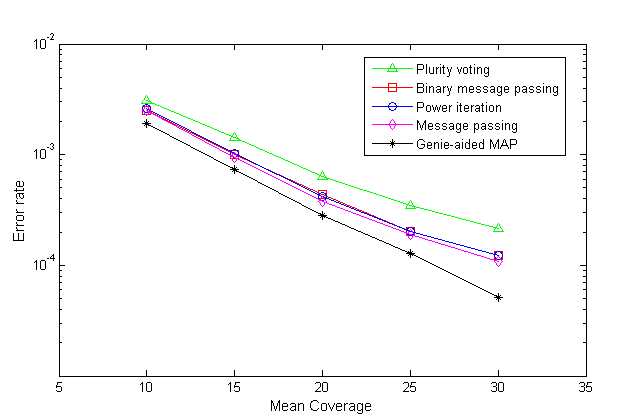
Figure 3: Error rates performance of the iterative learning schemes (message passing, binary message passing, and power iterations) compared with the plurality voting and genie-aided MAP schemes. The error rates of iterative learning schemes and plurality voting are averaged over $20$ experiments.

VI-B Experimental data

In addition to the simulation studies, we tested the performance of our proposed iterative learning schemes for reference-guided sequence assembly using two experimental data sets. In particular, we sequenced Escherichia Coli (from strain MG1655, $4.64\times 10^{6}$ bases long) and Neisseria Meningitidis (from strain FAM18, having length $2.2\times 10^{6}$) at the Center for Genomic Sequencing and Analysis of the University of Texas at Austin. The data is obtained using Illumina’s HiSeq platform that provides $100$bp-long paired-end reads, and the performance of our proposed methods are compared with that of the widely used sequencing analysis packages SAMtools and GATK. Both SAMtools and GATK process aligned next-generation sequencing data stored in SAM format, the alignment file format provided by the majority of frequently used alignment tools (e.g., BWA). These files contain the aligned reads, their positions and the quality scores of the bases. SAMtools calculates empirical quality scores from the alignment information and uses them to recalibrate the raw quality scores provided by the sequencing platform. The assembled sequence is formed using the aligned bases weighted by these new quality scores. In addition to the quality score recalibration, GATK also performs a local realignment procedure to correct misaligned reads, especially from the target genome region containing indels compared to the reference genome. After performing sequence assembly using quality score information, these software packages can also perform downstream single nucleotide polymorphism (SNP) detection, while GATK also incorporates a machine learning tool to separate true variation from sequencing platform artifacts.

The two genomes are sequenced using $67\%$ of an HiSeq platform lane having approximately $30\times 10^{6}$ reads, resulting in the coverage greater than $200$. This enables accurate inference of the true E. Coli and N. Meningitides sequences using any of the techniques discussed in the paper, providing us with the ground truth. To determine the accuracy of our proposed schemes in realistic scenarios where the coverage is limited, we uniformly subsample the data to emulate low coverage situations. The resulting error rates are shown in Table I. As can be seen there, the developed message passing schemes outperform both SAMtools and GATK in terms of the accuracy. The number of iterations for each message passing scheme was set to $30$, which at coverage $c=20$ resulted in the average CPU runtimes of $65$ and $37$ minutes for processing E. Coli and N. Meningitidis data sets, respectively (the algorithms were coded in C++, run on a 3.07G Hz single core machine). The corresponding runtimes for SAMtools are $50$ and $28$ minutes, and for GATK $53$ and $30$ minutes. As seen from the table, increasing the coverage can dramatically improve accuracy of the assembly – recall the discussion from Section V where we showed that the probability of error of the genie-aided MAP estimator decreases exponentially with the coverage. However, increasing coverage also increases the cost of the sequencing project.

Sequence	Number of errors
and Coverage	MP	BMP	SAMtools	GATK
E coli
15	$3484\pm 88$	$3507\pm 76$	$3655\pm 66$	$3598\pm 72$
20	$2566\pm 66$	$2599\pm 54$	$2677\pm 71$	$2634\pm 53$
25	$1243\pm 31$	$1256\pm 44$	$1298\pm 41$	$1283\pm 55$
30	$763\pm 20$	$781\pm 23$	$811\pm 23$	$798\pm 18$
N. Meningitidis
15	$2168\pm 35$	$2231\pm 43$	$2404\pm 37$	$2358\pm 30$
20	$1201\pm 29$	$1299\pm 26$	$1388\pm 30$	$1379\pm 20$
25	$899\pm 16$	$913\pm 20$	$933\pm 24$	$921\pm 19$
30	$658\pm 11$	$669\pm 11$	$681\pm 9$	$680\pm 15$

TABLE I: Performance of the message passing algorithm (MP), binary message passing algorithm (BMP), SAMtools and GATK on E. coli and N. Meningitidis sequencing data with various coverages. The average number of decision errors and the corresponding standard deviation are computed over $30$ runs.

Note that the sequenced genome might contain insertions as compared to the reference or, equivalently, the reference sequence contains gaps. This structural variation can be detected in the alignment stage by using paired-end reads [29], [30]. The paired-end reads have a known range of lengths of inserts between the reads in a pair. The gaps in the reference can be detected by relying on a multi-read alignment of the pairs of reads and comparing the aligned positions with the insert lengths. We used the scheme in [30] to perform the alignment of our E. Coli data set and detected $34$ gaps in the reference. We includes the gap positions as additional base nodes in our graphical model and uses our Algorithm 1 to identify the order of nucleotides in the gaps. As a result, $31$ out of $34$ gaps were reconstructed (i.e., closed).

VII Summary and Conclusion

We studied reference-guided sequence assembly from short reads generated by next-generation sequencing technologies, specifically focusing on the problem of obtaining the target genome sequence from potentially erroneous and misaligned reads. We cast the problem as the inference of the target sequence on an appropriately defined bipartite graph and proposed iterative learning algorithms for solving it. In particular, we developed message passing algorithms that rely on both binary as well as representation of nucleotide bases by $4$-dimensional vectors. It was shown that the derived message passing algorithm (in particular, Algorithm 1 in Section II) can be interpreted as the standard belief propagation under a certain prior. In addition, the problem was rephrased so that the power iteration algorithm, employed to find the leading singular vector of a matrix collecting all short reads, results in a good approximation of the target sequence. Convergence of power iterations is guaranteed, while the convergence of message passing algorithms is studied empirically. Unlike existing methods, the proposed algorithms find the desired sequence without using reliability information (i.e., quality scores) of the short reads – in fact, message passing algorithms infer the aforementioned quality score information.

To assess achievable accuracy of the proposed iterative learning techniques, we analyzed the probability of error of a genie-aided maximum a posteriori decision scheme in the idealized scenario where the base calling error rates and read mapping locations are known perfectly. It was shown empirically that the iterative learning schemes perform close to the genie-aided estimation scheme, and that they outperform state-of-the-art software packages for downstream processing of sequencing data.

References

- [1] J. Shendure and H. Ji, “Next-generation DNA sequencing,” Nat Biotechnology, vol. 26, pp. 1135-1145, 2008.
- [2] M. Metzker, “Emerging technologies in DNA sequencing,” Genome Research, vol. 56, pp. 1767-1776, 2005.
- [3] D. Bentley, “Whole-genome re-sequencing,” Curr Opin Genet Dev, vol. 16, pp. 545-552, 2006.
- [4] C. Ledergerber and C. Dessimoz, “Base-calling for next-generation sequencing platforms,” Brief Bioinformatics, 2011, 12(5):489-497.
- [5] W. Kao, K. Stevens, and Y. Song, “BayesCall: A model-based base-calling algorithm for high-throughput short-read sequencing,” Genome Research, vol. 19, pp. 1884-1895, 2009.
- [6] X. Shen and H. Vikalo, “ParticleCall: A particle filter for base calling in next-generation sequencing systems,” BMC Bioinformatics, vol. 13, July 2012.
- [7] S. Das and H. Vikalo, “Base calling for high-throughput short-read sequencing: Dynamic programming solutions,” BMC Bioinformatics, April 2013, 14:129, pp: 1-10.
- [8] R. Nielsen, J. S. Paul, A. Albrechtsen and Y. Song, “Genotype and SNP calling from next-generation sequencing data,”Nature Reviews Genetics, vol. 12, pp. 443-451, 2011.
- [9] A. Altmann, P. Weber, et al. “A beginners guide to SNP calling from high-throughput DNA-sequencing data,” Human Genetics, pp. 1-14, 2012.
- [10] R. Li, Y. Li, et al. “SNP detection for massively parallel whole-genome resequencing,” Genome Research, vol. 19: 1124-1132, 2009.
- [11] R. Dalloul, et al. “Multi-platform next-generation sequencing of the domestic turkey (Meleagris gallopavo): Genome assembly and analysis,” PLoS Biol, 8:e1000475, 2010.
- [12] R. Li, et al. “The sequence and de novo assembly of the giant panda genome,” Nature, vol. 463: 311-317, 2010.
- [13] H. Li, B. Handsaker, et al. “The Sequence Alignment/Map format and SAMtools,” Bioinformatics, vol. 25, pp. 2078-2079, 2009.
- [14] M. DePristo, E. Banks, R. Poplin, et al. “A framework for variation discovery and genotyping using next-generation DNA sequencing data,” Nature Genetics, vol. 43, pp. 491-498, 2011.
- [15] D. Smith, A. Quinlan, et al. “Rapid whole-genome mutational profiling using next-generation sequencing technologies,” Genome Research, vol. 18: 1638-1642, 2008.
- [16] B. Langmead et al. “Ultrafast and memory-efficient alignment of short DNA sequences to the human genome,” Genome Biology, vol. 10, 2009.
- [17] H. Li, R. Durbin, “Fast and accurate short read alignment with Burrows-Wheeler transform,” Bioinformatics, vol. 25, pp. 1754-1760, 2009.
- [18] R. M. Durbin et al. “A map of human genome variation from population-scale sequencing,” Nature 467 (7319): 10611073, 2010.
- [19] X. Shen and H. Vikalo, “A message-passing algorithm for reference-guided sequence assembly from high-throughput sequencing reads,” IEEE International Workshop on Genomic Signal Processing and Statistics (GENSIPS), December 2-4, 2012, Washington, DC, USA, pp: 35-37.
- [20] X. Shen, M. Shamaiah, and H. Vikalo, “Message-passing algorithm for inferring consensus sequence from next-generation sequencing data,” IEEE International Symposium on Information Theory, July 7-12, 2013, Istanbul, Turkey.
- [21] D. Karger, S. Oh, D. Shah, “Iterative learning for reliable crowd-sourcing systems,” in Proceedings of NIPS, 2011.
- [22] D. Karger, S. Oh, D. Shah, “Budget-optimal Crowdsourcing using Low-rank Matrix Approximation,” Communication, Control, and Computing (Allerton), 2011 49th Annual Allerton Conference on. IEEE, 2011.
- [23] J. Yedidia, W. Freeman, Y. Weiss, “Constructing free-energy approximations and generalized belief propagation algorithms,” IEEE Transactions on Information Theory, vol 51, pp. 2282-2312, 2005.
- [24] F. Kschischang and H. Loeliger, “Factor graphs and the sum-product algorithm,” IEEE Transactions on Information Theory, vol. 47, 2001.
- [25] X. Lin, S. Yacoub, J. Burns, and S. Simske, “Performance analysis of pattern classifier combination by plurality voting,” Pattern Recognition Letters, vol. 24, pp. 1959-1969, 2002.
- [26] W. C. Kao, A. H. Chan, and Y. S. Song, “ECHO: a reference-free short-read error correction algorithm,” Genome Research, vol. 21, no. 7, pp. 1181-92, 2011.
- [27] G. Levitin, Universal Generating Function in Reliability Analysis and Optimization, Springer-Verlag, 2005.
- [28] G. A. Churchill and M. S. Waterman, “The accuracy of DNA sequences: Estimating sequence quality,” Genomics, vol. 14, pp. 89-98, 1992.
- [29] DNASTAR: http://www.dnastar.com/t-sub-nextgen-genome-solutions-automated-genome-closure.aspx
- [30] T. Rausch, K. Sergey, et al. “A consistency-based consensus algorithm for de novo and reference-guided sequence assembly of short reads,” Bioinformatics, vol. 25, no. 9, pp. 1118-1124, 2009.