The available-enthalpy (flow-exergy) cycle.
Part-I: introduction and basic equations.

Abstract

A diagnostic package is derived from the concept of specific available enthalpy, leading to the definition of a local and complete energy cycle. It is useful to understand the transformations of energy occurring at any particular pressure level or pressure layer of a limited area domain. The global version of this diagnostic tool is very similar to the cycle of Lorenz, but the local counterpart contains several additional terms, with zonal, eddy and static-stability components close to definitions already given by Pearce. The new cycle takes into account the flow of energy components across the vertical and horizontal boundaries, with additional conversion terms involving potential energy, leading to accurate computations of dissipation and generation terms obtained as residuals. A new accurate temporal scheme is proposed in order to allow use of a large time interval in future numerical applications. Finally, comments are made on the arbitrary choice for two constant reference values for pressure and temperature.

1 Introduction.

Understanding of energy transformations occurring in the atmosphere is still a subject of research, and several methods exist to investigate observed atmospheric energetics. Margules (1905) performed an application to a single column of fluid, and its generalization to the general circulation has been realized by Lorenz (1955, hereafter L55). More recently, different local versions of the Lorenz cycle have been published when authors are concerned with small-scale phenomena like tropical or mid-latitude cyclogenesis, baroclinic-wave development or frontal cyclogenesis, all associated with limited-area domains (e.g. Muench 1965; Brennan and Vincent 1980; Michaelides 1987).

Previous local studies based on the Lorenz method have been able to catch the main features of local energy transformations, including usual baroclinic or barotropic conversions and involving classical differential heating terms, with boundary terms different from zero only in the case of limited-area domains.

However, these local versions lead to certain inconsistencies. There are two main problems resulting from global-scale assumptions that do not hold for limited-area domains. Firstly, all terms in the energy cycle are integrated part by part through the whole atmosphere and, as a consequence, finite vertical-extent domains or an isolated level cannot be considered. Secondly, the mean vertical velocity $\overline{\omega}\>=\>\overline{dp/dt}\>$, where $p$ is pressure, is supposed to cancel out when it is averaged over any horizontal layer. However this is only true for a surface surrounding the whole earth, which excludes the use of Lorenz’s cycle for local studies owing to large impacts caused by these approximations (Saltzman and Fleisher, 1960). For example, the mean conversion term $-\>R\>\overline{\omega}\>\overline{T}\>/{p}$ and eddy component $-\>R\>\overline{{\omega}^{\prime}\>{T}^{\prime}}\>/{p}$ can be of the same order of magnitude because, even if $|\overline{\omega}|$ is a tenth of $|{\omega}^{\prime}|$, $|\overline{T}|$ is commonly $10$ times greater than $|{T}^{\prime}|$ (Symbols are defined in appendix A). As a result, the mean conversion term cannot be neglected in limited-area energetics.

These local studies present other unrealistic features–for instance when dissipation and generation terms are the only unknown quantities and are computed as residuals of the cycle. It is often mentioned that these residuals are too large and that they lead to unbalanced terms, like the conversion terms with potential energy.

In other words, there is a need for a new kind of local energy cycle without any missing terms and where approximations would be overcome. The method adopted to revisit the approach of local energetics in meteorology is to start with a set of local and exact equations for temperature and wind, to define appropriate availability functions, to specify a reference state and finally to compute the average values over a given pressure level for a limited-area domain. This methodology ensures that all the terms will be present in the local version, even if some of these terms cease to exist in the globally averaged version.

A new local and exact available-enthalpy cycle is proposed in this paper. It will clear up the difficulties encountered with previous limited-area applications and, on the global stage, will lead to results more usually expected, including baroclinic and barotropic instabilities. This new cycle is based on the concept of available enthalpy described in Marquet (1991, hereafter M91), following the proposition of Sir Charles Normand (Normand 1946) when he chose a direct approach in terms of enthalpy (total heat) in place of the total potential energy used by Margules and Lorenz.

Part I of this paper was taken from a thesis (Marquet, 1994). The concept of available enthalpy has not been widely applied in meteorology and a short review of its development, both in meteorology and in general physics, will be discussed in the section 2. Kinetic-energy and available-enthalpy components are presented in section 3 and the fundamental energy equations are used in section 4 to define the limited-area available enthalpy cycle. Associated with this, a new accurate temporal scheme is proposed in section 5 to allow future use of large time intervals in Part II, where applications to idealized baroclinic waves will be presented. A discussion on the prescribed ‘reference’ pressure and temperature is presented in section 6. The final conclusion appears in section 7. Symbols and notations for Parts I and II are explained in Appendix A.

2 The energy availability concepts in meteorology and
thermodynamics.

2.1 In thermodynamics.

Problems of defining energy availability have been tackled in many ways in physics, and different available-energy and available-enthalpy concepts was developed during early developments in thermodynamics. The aim was to compute part of the total energy contained in a closed or open system that can be available for useful technical work. All availability functions introduced by Lord Kelvin (Thomson, 1849, 1853, 1879), Maxwell (1871) or Gibbs (1873) depend on the local internal energy ($e_{i}$), enthalpy ($h$) and entropy ($s$) of the fluid. A reference state must be specified, generally given by a constant ‘reference’ temperature ($T_{r}$) with associated pressure ($p_{r}$) and specific volume (${\alpha}_{r}$). There is only one available-enthalpy function:

$$a_{h}\;=\;(h-h_{r})\>-\>T_{r}\>(s-s_{r})\>,$$ (1)

but two available energies have been defined. Two functions, one simple and the other one more complex, are given by

$${a}_{e1}\;=\;[\>e_{i}-{(e_{i})}_{r}\>]\>-\>T_{r}\>(s-s_{r})\>,$$

and

$${a}_{e2}\;=\;[\>e_{i}-{(e_{i})}_{r}\>]\>+\>p_{r}\>({\alpha}-{\alpha}_{r})\>-\>T_{r}\>(s-s_{r})\>.$$

2.2 In meteorology.

Without referring to thermodynamic theories, and following the ideas of Margules, Lorenz defined available potential energy ($APE$) as the maximum part of the sum of internal and potential energies – also called total potential energy ($TPE$) – which can be transformed under adiabatic motion into kinetic energy ($K$). Margules and Lorenz treated kinetic energy as the useful energy in the atmosphere because of its easily visible effects. Lorenz’s approach can be summarized by a cycle (see Fig. 1), where each $APE$ and $K$ reservoirs are separated into two parts ($APE=AZ+AE$ and $K=KZ+KE$). The four components $AE$, $AZ$, $KE$ and $KZ$ correspond to a separation of the general circulation into zonally symmetric and eddy parts (denoted by the suffixes $Z$ and $E$ respectively). Energy generation terms $GE$ and $GZ$ provide energy to $AE$ and $AZ$, with dissipation terms $DE$ and $DZ$ acting on $KE$ and $KZ$. The terms $CA$, $CE$, $CK$ and $CZ$ are conversion terms as shown in Figure 1.

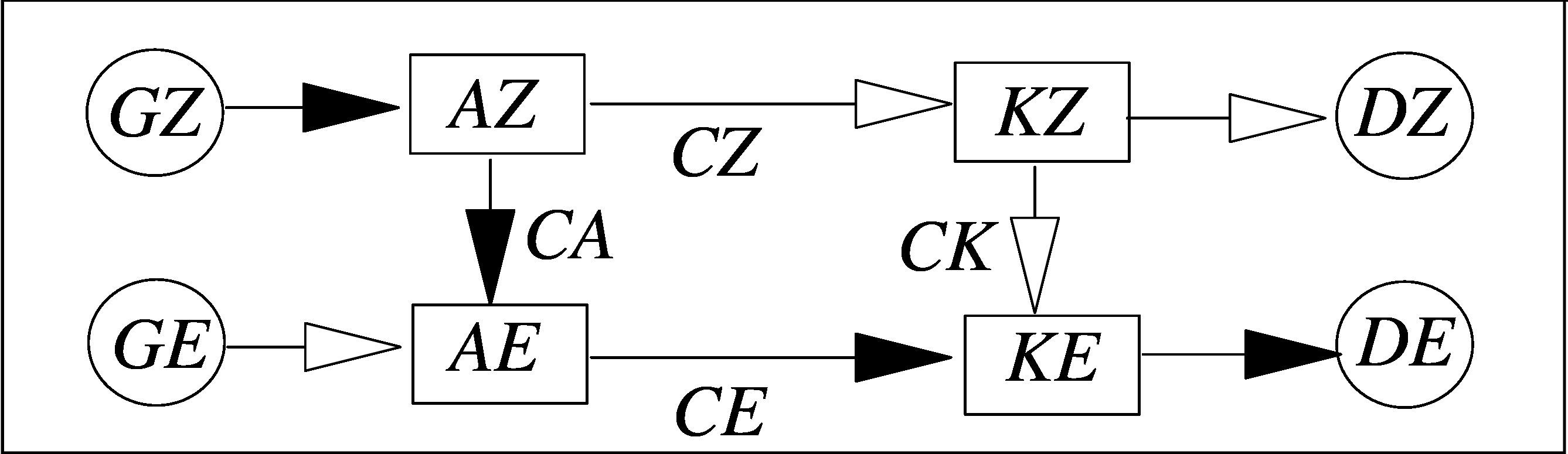
Figure 1: A diagram for the Lorenz cycle. The baroclinic instability is depicted by the dark arrows: $GZ\rightarrow\;$$CA\rightarrow\;$$CE\rightarrow\;$$DE$.

The result obtained by Lorenz demonstrates the maintenance of the general circulation ($KE$) by baroclinic instabilities ($CA$ and $CE$). The horizontal differential heating term $GZ$ supplies energy to the internal reservoir $AZ$ which is transformed into kinetic energy by baroclinic conversions $CA$ and $CE$, so that the $KE$ component is maintained despite the continuous dissipation $DE$.

Apart from the global Lorenz cycle and associated local versions, other availability functions have been defined in meteorology. It has been demonstrated in Marquet (1995) that most of them are associated with special thermodynamic availability functions. For instance, the available energy ${a}_{e1}$ corresponds to a quantity $T_{0}\Sigma$ called ‘static entropic energy’. Defined by Eq. (51) in the global approach of Dutton (1973), it is also the available energy examined in the production of a local version of Dutton’s theory by Pichler (1977). The function ${a}_{e2}$ is equivalent to another form of ‘static entropic energy’ described by Livezey and Dutton (1976). Furthemore, it is also the dry part of the ‘exergy’ function suggested by Karlsson (1990). Even if the exergy term is a generic name used in modern thermodynamics to denote any of the availability functions ${a}_{e1}$, ${a}_{e2}$ or $a_{h}$, depending on the system to be investigated, the terms ‘available energy’ or ‘available enthalpy’ will be used in this paper.

The previous relationship between the thermodynamic availability functions ${a}_{e1}$ or ${a}_{e2}$ and their meteorological counterparts has already been stated in M91, where a possible application of a local available-enthalpy function $a_{h}$ to atmospheric energetics was also considered, but where the local cycle was not derived. It was mentioned that the theory of $APE$ presented in Pearce (1978, hereafter P78) was the first application of the available-enthalpy concept to atmospheric science. Pearce defined the global $APE$ function such that $d/dt(APE)=d/dt(H-T_{r}S)$ applies to the whole atmosphere, with $T_{r}\approx 251$ K. Clearly, the global available enthalpy

$$A_{h}\>=\>(H-T_{r}\>S)\>-\>(H_{r}-T_{r}\>S_{r})$$

is a solution to this equation, but the constant term $H_{r}-T_{r}S_{r}$ was missing in the paper of Pearce and his following mathematical developments were carried out using several approximations that will be overcome in this paper.

Other approaches have also been proposed in meteorology to generalize the results of Lorenz, though most of them have not succeeded in deriving a set of energy equations similar to the Lorenz cycle. The same is also true for the local and positive-definite potential energy of Andrews (1981) - see section 6 in Part-I of this paper for further explanations –, for the $APE$ of MacHall (1990), or for the local pseudo-energy concept of Shepherd (1993) – a generalization of all meteorological availability functions – also discussed in Kucharski (1997). As demonstrated by Marquet (1995), it is possible to deduce Lorenz, Dutton or Pearce’s results by choosing, for each case, an appropriate reference state in the pseudo-energy theory. However, up to now, it appears that no general cycle has been published starting with this concept.

2.3 The available enthalpy function

The basis for the research presented in this paper can be found in the thesis report of Marquet’s (1994). However, several theoretical improvements and some new applications will be included in this article. An approach similar to P78 will be retained by separating $A_{h}$ into three energy components, depending on pressure averages for $A_{S}$, zonally symmetric circulations for $A_{Z}$ and eddy circulations for $A_{E}$. Kinetic energy will also be separated into three parts $K_{S}$, $K_{Z}$ and $K_{E}$, contrary to L55 and P78 when $K_{S}$ and $K_{Z}$ were merged into a single component, also called $K_{Z}$. The new proposal is an available enthalpy cycle with $A3+K3$ components ($3$ for the thermal part and $3$ for the kinetic part), substituting $A2+K2$ in L55 and $A3+K2$ in P78.

3 Energy components.

3.1 Local available enthalpy $a_{h}$.

According to M91, available enthalpy per unit mass ‘$a_{h}$’ defined by (1) is equal to $(h-h_{r})-T_{r}\>(s-s_{r})$. Therefore it only depends on differences in enthalpy and entropy which only depends on local temperature ($T$) and pressure ($p$):

$$h-h_{r} =\;c_{p}\>(T-T_{r})\>,$$ (2)

$$s-s_{r} \;=\;c_{p}\>\ln\left\{\left(\frac{T}{T_{r}}\right)\left(\frac{p}{p_{r}}\right)^{-{\kappa}}\right\}\;=\;c_{p}\>\ln\left(\frac{T}{T_{r}}\right)\>-\>R\>\ln\left(\frac{p}{p_{r}}\right)\>.$$ (3)

Note that absolute values for enthalpy $h$ or even entropy $s$ need not be known, only the relative differences (2) and (3) are required for determining $a_{h}$. The reference temperature and pressure $T_{r}$ and $p_{r}$ are chosen as two constants in space and time. Following M91, $1/T_{r}$ and $\ln(p_{r})$ should be global and long-range averages of $1/T$ and $\ln(p)$, respectively. In fact, two prescribed numerical values, set to $250$ K for $T_{r}$ and $1000/\exp(1)\approx 368$ hPa for $p_{r}$, will be used in this paper. It will be demonstrated later that results will not be affected when the reference values are perturbed.

According to M91, the available enthalpy (1) can be separated into a sum of two local components $a_{T}$ and $a_{p}$, the first one depending on temperature, the other one on pressure, to give

$$a_{h}\>(T,p\>;\>T_{r},p_{r}) = a_{T}\>(T\>;\>T_{r})\>+\>a_{p}\>(p\>;\>T_{r},p_{r})\>,$$ (4)

where

$$a_{T}\;=\;c_{p}\;T_{r}\>{\cal F}(X)\>,\hskip 39.83368pta_{p}\;=\;R\>\>T_{r}\>\ln(p/p_{r})\>,$$ (5)

$${\cal F}(X)\>=\>X-\ln(1+X)\>,\hskip 11.38092ptX(T,T_{r})\;=\;\frac{T-T_{r}}{T_{r}}\;=\;\frac{T}{T_{r}}-1\>.$$ (6)

The local temperature component $a_{T}$ is written with the help of a function ${\cal F}$ defined by (6) for any variable $X>-1$. Function ${\cal F}$ also verifies the exact separating property (7) that holds whenever $X_{1}>-1$ and $X_{2}>-1$ (in which case $X_{1}+X_{2}+X_{1}\>X_{2}=(1+X_{1})\>(1+X_{2})-1$ is also greater than $-1$):

$${\cal F}(X_{1}+X_{2}+X_{1}\>X_{2})\!\! = \!\!{\cal F}(X_{1})\;+\;{\cal F}(X_{2})\;+\;X_{1}\>X_{2}\>.$$ (7)

Function ${\cal F}$ is a positive, quadratic function for small $|X|$, as indicated by the expansions (8) and (10). Typically, $|X|<0.3$ for $T_{r}\equiv 250$ K and for temperatures between $320$ K and $180$ K, as observed in usual atmospheric conditions.

$${\cal F}(X)\!\! = \!\!\frac{X^{2}}{2}\;-\;\frac{X^{3}}{3}\;+\;o(X^{3})\>,$$ (8)

$$\Rightarrow{\cal F}(X)\!\! \approx \!\!{\cal G}(X)\>=\>\frac{X^{2}}{2}\hskip 17.07182pt\hbox{for }\;|X|\;\approx 0\>,$$ (9)

$${\cal F}(\alpha\>X)\!\! = \!\!{\alpha}^{2}\>{\cal F}(X)\;-\;{\alpha}^{2}\>(\alpha-1)\>\frac{X^{3}}{3}\;+\;o(X^{3})\>.$$ (10)

As a consequence, ${\cal G}$ given by (9) is a good approximation of ${\cal F}$ for small $|X|$, and the temperature component (5) is found to be similar to the local function ‘$a$’ in P78. The result is $a_{T}\approx a=c_{p}\>{(T-T_{r})}^{2}/(2\>T_{r})$.

3.2 Limited area components for $a_{h}$ and $e_{k}$

According to L55 and the following limited-area applications of Muench (1965), Brennan and Vincent (1980), P78 and Michaelides (1987), the eddy part of the flow will be computed by a departure from the zonal average circulation, when the zonal average is defined over the limited area domain. The notations for the isobaric $\overline{(...)}$ and zonal ${(...)}^{\lambda}$ averaging operators are described in Appendix-A, where superscripts and subscripts (for instance $T^{\lambda}=T-T_{\lambda}$) represent average values and deviations from them, respectively.

It is expected that $a_{T}$ can be separated into the three local components of P78, $a_{S}$, $a_{Z}$ and $a_{E}$, possibly with further local terms. A concise description will be obtained in terms of the function ${\cal F}$ of $X_{S}$, $X_{B}$, $X_{Z}$ and $X_{E}$. The final result will be obtained with the property (7) applied successively to the exact separations

$$\left(\frac{T}{T_{r}}-1\right)\; = \;\;\left(\frac{T}{\overline{T}}-1\right)\;\;+\;\left(\frac{\overline{T}}{T_{r}}-1\right)\;\;+\;\left(\frac{T}{\overline{T}}-1\right)\left(\frac{\overline{T}}{T_{r}}-1\right)\>,$$ (11)

$$\left(\frac{T}{\overline{T}}-1\right)\; = \;\left(\frac{T}{{T}^{\lambda}}-1\right)\;+\;\left(\frac{{T}^{\lambda}}{\overline{T}}-1\right)\;+\;\left(\frac{T}{{T}^{\lambda}}-1\right)\left(\frac{{T}^{\lambda}}{\overline{T}}-1\right)\>.$$ (12)

Equations (11) and (12) can be understood as an insertion of $\overline{T}$ between $T$ and $T_{r}$ for (11), and an insertion of ${T}^{\lambda}$ between $T$ and $\overline{T}$ for (12). Note that these equations are directly put in the form $X_{1}+X_{2}+X_{1}\>X_{2}$ as required by (7).

After some manipulations, it is found that the temperature component $a_{T}$ can indeed be written as a sum of the local version of Pearce components $a_{S}$, $a_{Z}$ and $a_{E}$, with two additional terms $a_{cS}$ and $a_{cZ}$, to give

$$a_{T}\!\! = \!\!\>a_{S}\>+\>a_{Z}\>+\>a_{E}\>+\>a_{cS}\>+\>a_{cZ}\>,$$ (13)

where

$$a_{S}\;=\;c_{p}\;T_{r}\;{\cal F}(X_{S})\>,\;\;\;\;\;a_{Z}\;=\;c_{p}\;T_{r}\;{\cal F}(X_{Z})\>,\;\;\;\;\;a_{E}\;=\;c_{p}\;T_{r}\;{\cal F}(X_{E})\>,$$ (14)

and

$$a_{cS}\;=\;c_{p}\;T_{r}\;X_{S}\;X_{B}\>,\;\;\;X_{S}\;=\;\frac{{\overline{T}-T_{r}}}{T_{r}}\>,\;\;\;X_{B}\;=\;\frac{T-\overline{T}}{\overline{T}}\>,$$ (15)

$$a_{cZ}\;=\;c_{p}\;T_{r}\;X_{Z}\;X_{E}\>,\;\;\;X_{Z}\;=\;\frac{{T}^{\lambda}-\overline{T}}{\overline{T}}\>,\;\;\;X_{E}\;=\;\frac{T-{T}^{\lambda}}{{T}^{\lambda}}\>,$$ (16)

or, alternatively,

$$X_{B}\;=\;\frac{T^{\>\prime}}{\overline{T}}\>,\;\;\;\hskip 31.2982ptX_{Z}\;=\;\frac{{T}^{\lambda}_{\varphi}}{\overline{T}}\>,\;\;\;\hskip 31.2982ptX_{E}\;=\;\frac{{T}_{\lambda}}{{T}^{\lambda}}\>.$$ (17)

The function ${\cal F}(X)$ is always positive and equal to zero only if $X=0$. This property can be applied to the mean values $\overline{a_{S}}$, $\overline{a_{Z}}$ and $\overline{a_{E}}$ which differ from zero only if $\overline{T}\neq T_{r}$, ${T}^{\lambda}\neq\overline{T}$ and $T\neq{T}^{\lambda}$, respectively.

The components of Pearce are obtained as approximate forms of Eqs. (14) when ${\cal F}$ is replaced by ${\cal G}$, together with the hypotheses ${(T_{r}/\overline{T})}^{2}\approx 1$ and ${(T_{r}/{T}^{\lambda})}^{2}\approx 1$, giving

$$a_{S}\;\approx\;c_{p}\;\frac{\left(\overline{T}-T_{r}\right)^{2}}{2\>T_{r}}\;,\hskip 14.22636pta_{Z}\;\approx\;c_{p}\;\frac{\left({T}^{\lambda}_{\varphi}\right)^{2}}{2\>T_{r}}\;,\hskip 14.22636pta_{E}\;\approx\;c_{p}\;\frac{\left({T}_{\lambda}\right)^{2}}{2\>T_{r}}\>.$$ (18)

The three components $a_{S}$, $a_{Z}$ and $a_{E}$ have been called in P78, ‘static stability’, ‘zonal’ and ‘eddy’ reservoirs, respectively. The new component $a_{p}$ given by (5) and the two complementary parts $a_{cS}$ and $a_{cZ}$ in (13) were missing in P78. There was no impact on the global scale since the vertical integral of $a_{p}$ and the horizontal average $\overline{a_{cS}}$ and $\overline{a_{cZ}}$ are $0$. But, for a limited area study, the flux of these additional components $\overline{B(a_{p})}$, $\overline{B(a_{cS})}$ and $\overline{B(a_{cZ})}$ are non zero and cannot be neglected.

It is also possible to separate the kinetic energy $e_{k}={\bf U}_{h}.{\bf U}_{h}/2$ into three components $k_{S}$, $k_{Z}$ and $k_{E}$, with two additional parts $k_{cS}$ and $k_{cZ}$, giving

$$e_{k} =\;k_{S}\;+k_{Z}\;+\;k_{E}\;+\;k_{cS}\;+\;k_{cZ}\>,$$ (19)

where

$$k_{S} =\;\frac{(\overline{u}){}^{2}+(\overline{v}){}^{2}}{2}\>,\hskip 14.22636ptk_{Z}\;=\;\frac{({u}^{\lambda}_{\varphi}){}^{2}+({v}^{\lambda}_{\varphi}){}^{2}}{2}\>,\hskip 14.22636ptk_{E}\;=\;\frac{({u}_{\lambda}){}^{2}+({v}_{\lambda}){}^{2}}{2}\>,$$ (20)

$$k_{cS} =\;u^{\prime}\>\overline{u}\;+\;v^{\prime}\>\overline{v}\>\>,\hskip 11.38109ptk_{cZ}\;=\;\>{u}^{\lambda}_{\varphi}\;{u}_{\lambda}\;+\;{v}^{\lambda}_{\varphi}\;{v}_{\lambda}\>\>.$$ (21)

An exact separating property (22) observed for the quadratic function ${\cal G}(X)=X^{2}/2$, equivalent to (7) observed for ${\cal F}(X)=X-\ln(1+X)$ and $a_{h}$, has been used to derive (20)-(21):

$${\cal G}(X_{1}+X_{2})\!\! = \!\!{\cal G}(X_{1})\;+\;{\cal G}(X_{2})\;+\;X_{1}\>X_{2}\>.$$ (22)

3.3 Interpretations for the limited-area components.

The six components ($a_{S}$, $a_{Z}$, $a_{E}$) and ($k_{S}$, $k_{Z}$, $k_{E}$) are little known in atmospheric energetics. Even if the three available-enthalpy reservoirs are similar to the components defined in P78, results published in the global approach of Pearce have not been widely applied in meteorology and it is worthwhile to explore further their physical meaning, especially for a limited-area domain. The same is true for the separation of $e_{k}$ into three components where the eddy part, $k_{E}$, is the only part not to undergo a redefinition ; it is defined as usual. The large-scale parts $k_{Z}$ and $k_{S}$ correspond to a new approach justified for the sake of retaining symmetry between the two sets of components.

(a)    $\overline{T}-T_{r}$ for $a_{S}$                                     (b)    ${T}({\lambda},{\varphi})$                  

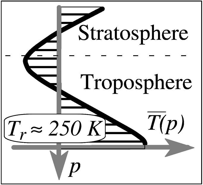
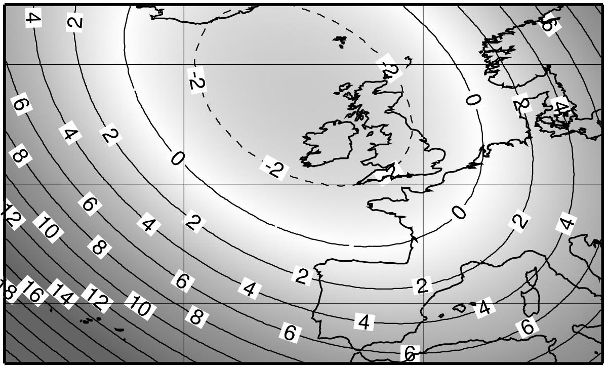
(c)    ${T}^{\lambda}_{\varphi}$ for $a_{Z}$                                             (d)    ${T}_{\lambda}$ for $a_{E}$

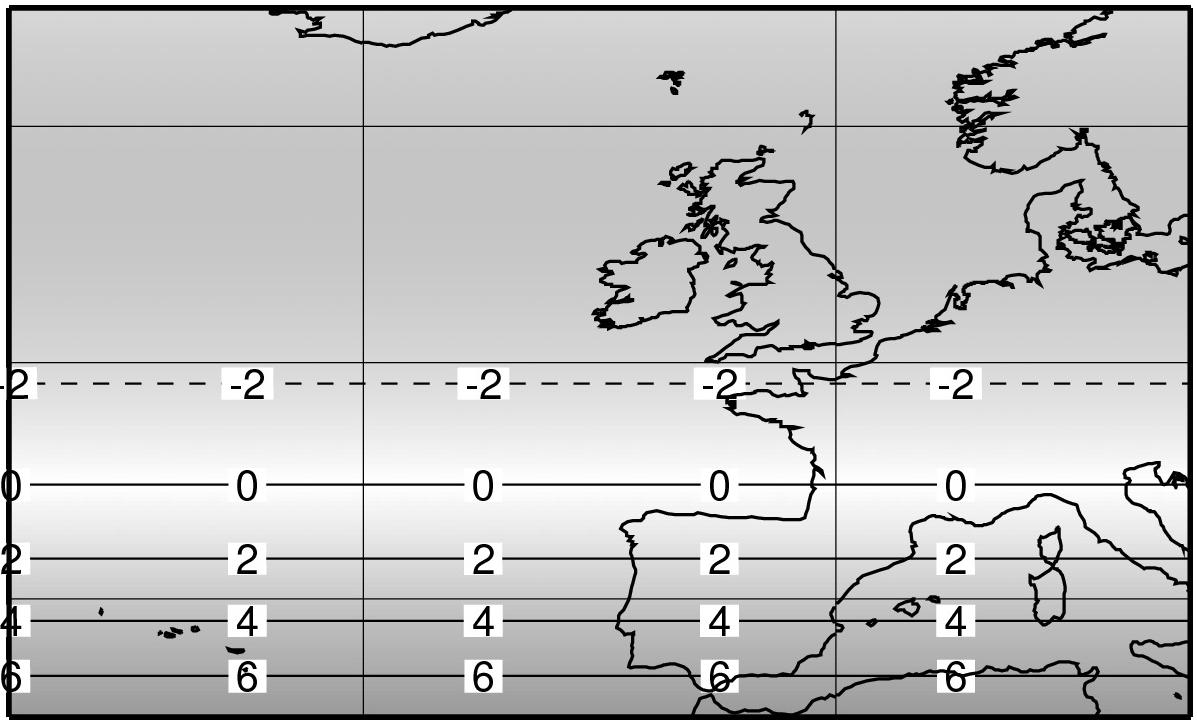
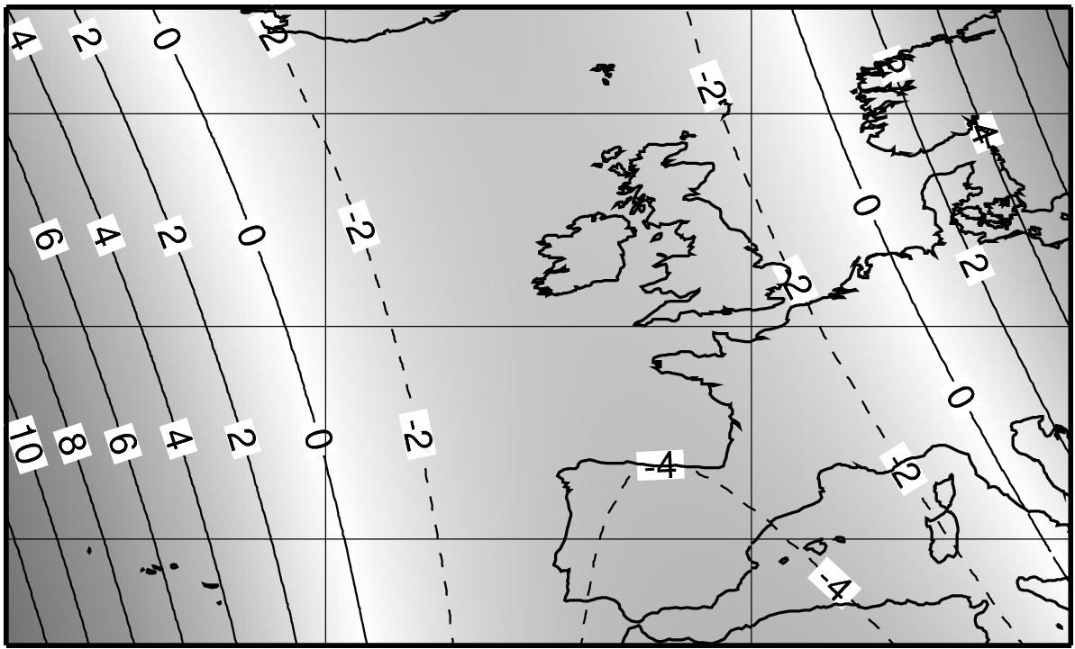
Figure 2: The separation of $\overline{a_{T}}$ (the thermal part of the available enthalpy $\overline{a_{h}}$ ) into $\overline{a_{S}}\>+\>\overline{a_{Z}}\>+\>\overline{a_{E}}$. (a) Values of $\overline{T}-T_{r}$ for $a_{S}$. (b) A temperature distribution made of a cold minimum located within a limited area domain. (c) Values of ${T}^{\lambda}_{\varphi}$ for $a_{Z}$. (d) Values of ${T}_{\lambda}$ for $a_{E}$. See text for further explanation.

An example of $\overline{a_{T}}$ separation is shown on Fig. 2. Following Pearce, ‘$a_{S}$’ will be called the vertical ‘static stability’ component and according to Fig. 2(a) is the part of thermal availability created by the difference between the average vertical profile $\overline{T}$ and a constant prescribed profile $T_{r}$ (shaded area). The horizontal separation of $\overline{a_{T}}$ into $\overline{a_{Z}}+\overline{a_{E}}$ is illustrated by the use of a simulated temperature distribution, described in Fig. 2(b). It is an elongated cold minimum with a north-west to south-east orientation and the minimum is not centred with respect to the limited area domain. Figure 2(c) shows how the component $a_{Z}$ is created by the north/south differences in zonal average temperature ${T}^{\lambda}_{\varphi}={T}^{\lambda}-\overline{T}$. The isopleths in Fig. 2(d) represent the distribution of the zonal departure ${T}_{\lambda}=T-{T}^{\lambda}$ which generates the eddy component $a_{E}$. Even if the east/west gradient prevails, it is found that the north-west to south-east tilted feature is still present.

The old Lorenz partitioning $APE=A_{Z}+A_{E}$ corresponds to a mixing of horizontal and vertical departure terms defined by the integrands ${T}^{\lambda}_{\varphi}/\overline{\sigma}$ and ${T}_{\lambda}/\overline{\sigma}$, respectively, where $\overline{\sigma}$ is the mean static stability. The numerators for these integrands are represented on Fig. 2(c) and (d) for ${T}^{\lambda}_{\varphi}$ and ${T}_{\lambda}$, respectively. The common denominator $\overline{\sigma}$ depends on the mean vertical lapse rate and can be compared to some extent with the component $a_{S}$ which depends on $\overline{T}-T_{r}$. However an important result is that the component $a_{S}$ is still valid for hydrostatically neutral or unstable states when local values of $\sigma$ are close to zero or negative, in which case local values of Lorenz’s components depending on $\overline{\sigma}$ become infinite and meaningless.

(a)    Wind ($u$, $v$) for $e_{k}$

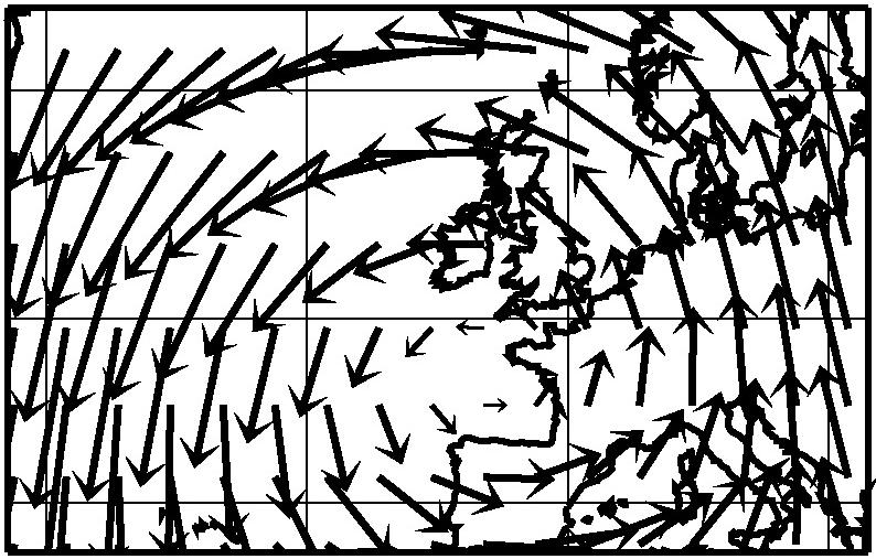
(b)    (${u}_{\lambda}$, ${v}_{\lambda}$) for $k_{E}$                                         (c)    (${u}^{\lambda}_{\varphi}$, ${v}^{\lambda}_{\varphi}$) for $k_{Z}$
                 
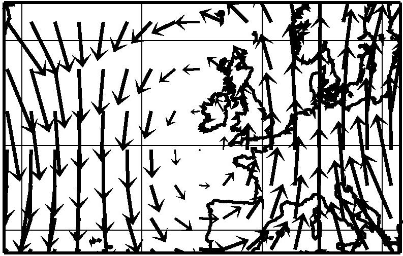
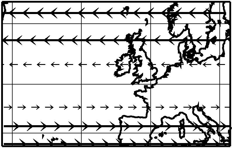
                  (d)    ($\overline{u}$, $\overline{v}$) for $k_{S}$                            (e)    Lorenz and Pearce ‘${K_{Z}}$’$\>=k_{S}+k_{Z}$
                 

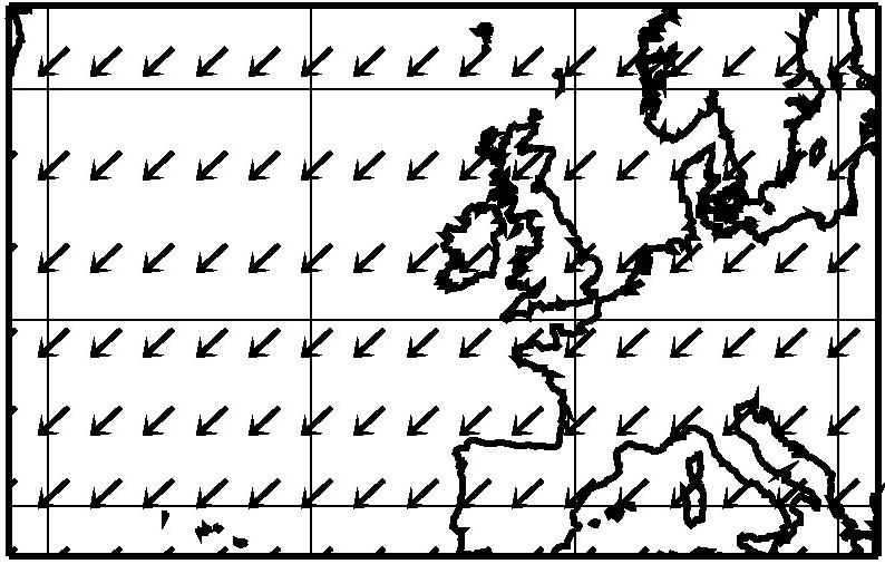
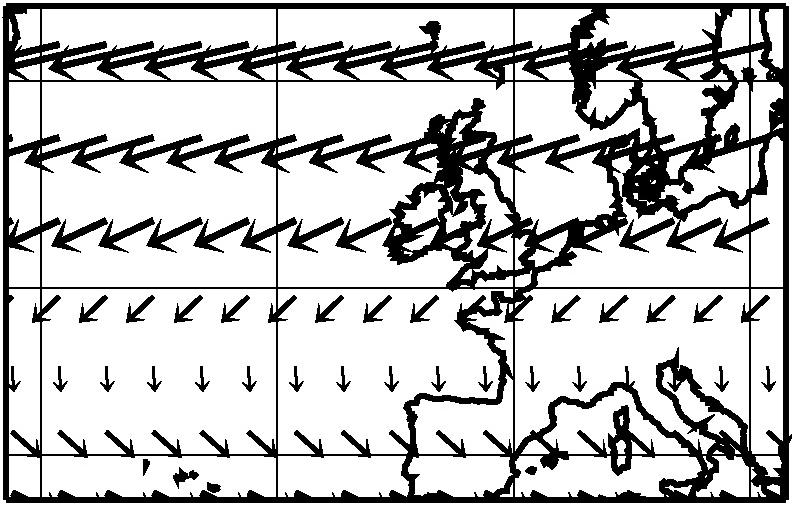
Figure 3: An illustration for the separation (19) applied to a simulated vortex within a limited area domain. The separation $\overline{e_{k}}=\overline{k_{S}}+\overline{k_{Z}}+\overline{k_{E}}$ proposed in this paper is shown in (b), (c) and (d). Lorenz’s and Pearce’s large scale version $\overline{k_{S}}+\overline{k_{Z}}$ is depicted in (e). (a) The map for the local wind ($u$, $v$). (b) The wind (${u}_{\lambda}$, ${v}_{\lambda}$) for $k_{E}$. (c) The wind (${u}^{\lambda}_{\varphi}$, ${v}^{\lambda}_{\varphi}$) for $k_{Z}$. (d) The wind ($\overline{u}$, $\overline{v}$) for $k_{S}$. (e) Lorenz and Pearce large scale component for the wind (${u}^{\lambda}$, ${v}^{\lambda}$) for $k_{S}+k_{Z}=\>$‘${K_{Z}}$’. See text for further explanation.

Figure 3 shows the new separation of $\overline{e_{k}}$ into $\overline{k_{E}}+\overline{k_{Z}}+\overline{k_{S}}$ when it is applied to a simulated vortex not centred with respect to the limited-area domain. The local wind vectors corresponding to components $k_{E}$, $k_{Z}$ and $k_{E}$ are depicted by Figure 3 (b), (c) and (d), respectively. The eddy-vortex part of the flow is clearly captured by Figure 3 (b) (${u}_{\lambda}$ and ${v}_{\lambda}$). Furthermore, large scale shearing of the zonal average wind can be recognized on Figure 3 (c) (${u}^{\lambda}_{\varphi}$ and ${v}^{\lambda}_{\varphi}$). The third component $k_{S}$ corresponds to the uniform average motion $\overline{u},\overline{v}$. The wind field representation, $k_{Z}+k_{S}$ (depicted on Fig. 3(e)), is the component referred to as ‘$K_{Z}$’ by Lorenz and Pearce. For this particular flow in this limited area, a large scale vortex feature is visible for ‘$K_{Z}$’ and it is redundant with the $k_{E}$ information. Moreover, the average motion picture shown on Fig. 3(d) is not easily identified in Fig. 3(e). For these reasons, the new separation into the three components $\overline{k_{E}}+\overline{k_{Z}}+\overline{k_{S}}$ as proposed in this study seems to be appropriate to catch relevant spatial scales for such a vortex motion.

4 The limited-area available enthalpy cycle.

4.1 Basic equations.

The available-enthalpy cycle will be reproduced as a set of six equations for the six available-enthalpy and kinetic-energy components. Pressure coordinates will be used with vertical velocity $\omega=d/dt(p)$ according to Kasahara (1974). The Eulerian time derivative operator $\partial/\partial t$ will be applied to each of the six components and will be expressed by using the material derivative $d/dt$ and a boundary function $B$. The resulting operator is given for any scalar $\eta$ as

$$\frac{\partial\,\eta}{\partial\,t} = \frac{d\,\eta}{d\,t}\>-\>B(\eta)\>,$$ (23)

where

$$B(\eta) = {{\rm div}\,}_{\!\!p}\>(\eta\>{\bf U}_{h}\>)\;+\;\frac{\partial}{\partial\,p}\left(\eta\>\omega\right)\;=\;{\bf U}_{h}\>.\>{\bf\nabla}_{\!p}\>(\eta)\;+\;\omega\;\frac{\partial\,\eta}{\partial\,p}\>,$$ (24)

$$\mbox{with}\hskip 28.45274ptB(\phi) = {\bf U}_{h}\>.\>{\bf\nabla}_{\!p}\>(\phi)\;-\;\frac{R}{p}\;\omega\>T\>.$$ (25)

The hydrostatic assumption and continuity equations will be used in the forms:

$$\frac{\partial\,\phi}{\partial\,p}\;=\;-\;\frac{R\>T}{p}\hskip 19.91684pt\mbox{and}\hskip 19.91684pt0\;=\;{{\rm div}\,}_{\!p}\>({\bf U}_{h}\>)\;+\;\frac{\partial\,\omega}{\partial\,p}\>.$$ (26)

The two representations of $B(\eta)$ in Eq. (24) in terms of divergence or gradient operators are equivalent, linked by the continuity equation. The special case for $B(\Phi)$ in Eq. (25) is obtained when the hydrostatic assumption is taken into account.

The momentum and thermodynamic equations as used in the Eulerian version of the French Arpege model can be written as follows (Courtier et al., 1991) :

$$\frac{d\,{\bf U}_{h}}{d\,t}\! = \!-\>{\bf\nabla}_{\!p}(\phi)\;-\;f\>{\bf k}\times{\bf U}_{h}\;+\;{\bf F}_{h}\>,$$ (27)

$$\frac{d\,u}{d\,t}\! = \!-\>[{\bf\nabla}_{\!p}(\phi)]{}_{x}\;+\;f^{\ast}v\;+\;({F}_{h}){}_{x}\>,$$ (28)

$$\frac{d\,v}{d\,t}\! = \!-\>[{\bf\nabla}_{\!p}(\phi)]{}_{y}\;-\;f^{\ast}u\;+\;({F}_{h}){}_{y}\>,$$ (29)

$$c_{p}\;\frac{d\,T}{d\,t}\! = \!\;\frac{R}{p}\;\omega\>T\;+\;\dot{q}\>,$$ (30)

where friction (${\bf F}_{h}$) and diabatic heating ($\dot{q}$) are forcing terms. The pseudo-Coriolis factor $f^{\ast}$ is the sum of the usual Coriolis ($f=2\>\Omega\sin(\varphi)$) term and horizontal curvature, giving $f^{\ast}=f+u\tan(\varphi)/{\cal R}$.

4.2 The energy equations.

The kinetic energy equation per unit mass is easily obtained for

$$e_{k}\;=\;\frac{1}{2}\;{\bf U}_{h}\,.\,{\bf U}_{h}\;=\;\frac{1}{2}\;\left(u^{2}+v^{2}\right)$$

by taking the dot product of Eq. (27) by ${\bf U}_{h}$, to get

$$\frac{d\,e_{k}}{d\,t} = -\>{\bf U}_{h}\>.\>{\bf\nabla}_{\!p}\>(\phi)\;+\;{\bf U}_{h}\>.\>{\bf F}_{h}\;=\;-\>B(\phi)\;-\;\frac{R}{p}\;\omega\>T\>-\;d\>.$$ (31)

The frictional dissipation $d$ denotes the scalar product $-{\bf U}_{h}\>.\>{\bf F}_{h}$ and the Coriolis term does not contribute to any local exchange of energy. The second formulation for (31) is a consequence of Eq. (25) by which $-\>{\bf U}_{h}\>.\>{\bf\nabla}_{\!p}\>(\phi)$ can be transformed into $-\>B(\phi)-R\>\omega\>T/{p}$.

The potential-energy equation per unit mass satisfies

$$\frac{d\,\phi}{d\,t} = \frac{\partial\,\phi}{\partial\,t}\>+\>B(\phi)\>.$$ (32)

The entropy equation is deduced from $s=s_{00}+c_{p}\ln\{(T/T_{00}){(p/p_{00})}^{-R/c_{p}}\}$ and used with Eq. (30), to give:

$$T\;\frac{d\,s}{d\,t} = c_{p}\;\frac{d\,T}{d\,t}\;-\;\frac{R}{p}\;\omega\>T\;\;\;=\;\;\;\dot{q}\>.$$ (33)

An equation for $a_{h}$ is then obtained by applying the Eulerian time derivative operator to (1) with the use of (30) and (33), whilst remembering the fact that the material derivatives of constant terms $T_{r}$ and $p_{r}$ cancel out. The result is

$$\frac{d\,a_{h}}{d\,t} = c_{p}\left(1-\frac{T_{r}}{T}\right)\>\frac{d\,T}{d\,t}\>+\>\frac{R}{p}\;\omega\>T_{r}\;=\;\frac{R}{p}\;\omega\>T\>+\>\left(1-\frac{T_{r}}{T}\right)\>\dot{q}\>.$$ (34)

The final term in (34) is a generation of available enthalpy by diabatic heating $\dot{q}$ with a modulation by the local efficiency factor $(1-T_{r}/T)$, also called the Carnot factor in thermodynamics. The sign of this factor is the same as that of ($T-T_{r}$), but the sign of the complete term $(1-T_{r}/T)\>\dot{q}$ depends on the correlation between $(1-T_{r}/T)$ and $\dot{q}$. The last term in (34) is interpreted as a generation by horizontal and vertical differential heating, as in L55 and P78.

The available enthalpy equation (34) is associated with a local law of conservation, valid along any streamline. The change in time of the sum $a_{k}+e_{k}+\phi$ is evaluated from (31), (32) and (34), to give

$$\frac{d}{d\,t}\left(\>a_{h}+e_{k}+\phi\>\right) = \frac{\partial\,\phi}{\partial\,t}\>+\>\left(1-\frac{T_{r}}{T}\right)\>\dot{q}\;-\;d\>.$$ (35)

As a result, the sum ($\>a_{k}+e_{k}+\phi\>$) is a constant along any particular streamline for a frictionless and isentropic steady flow. It is Bernoulli’s law, valid for the available enthalpy. The only difference from the usual Bernoulli’s equation observed for the sum $(\>h+e_{k}+\phi\>)$ is the Carnot’s Factor $(1-{T_{r}}{/T})$ in factor of the heating rate $\dot{q}$.

4.3 The limited-area available-enthalpy cycle.

The budget equations for the new available-enthalpy cycle are obtained by computing the time derivatives of the six components $a_{S}$, $a_{Z}$, $a_{E}$, $k_{S}$, $k_{Z}$ and $k_{E}$. This requires considerable manipulations based on the definitions given in the previous sections and in the Appendix-A. There is no approximation, no development in series and no missing terms. An example of the beginning of the $a_{Z}$ computations is presented in Appendix-B. All terms are rearranged to reproduce the form of classical results for the main global-scale conversion, generation and dissipation terms. The final result is as follows

$$\left.\begin{aligned} \overline{{\partial}_{t}(a_{S})}\;&\>=\;\;-\;\overline{B(a_{S}+a_{cS})}\;-\;\overline{c_{AS}}\;-\;\overline{c_{S}}\mbox{\hskip 34.14322pt}\;-\;\overline{B(a_{p})}\mbox{\hskip 2.84544pt}\;+\;\overline{g_{S}}\vspace*{-0.4 cm}\\ \overline{{\partial}_{t}(a_{Z})}\;&\>=\;\;-\;\overline{B(a_{Z}+a_{cZ})}\;+\;\overline{c_{AS}}\;-\;\overline{c_{Z}}\;-\;\overline{c_{A}}\mbox{\hskip 48.36958pt}\;+\;\overline{g_{Z}}\vspace*{-0.4 cm}\\ \overline{{\partial}_{t}(a_{E})}\;&\>=\;\;-\;\overline{B(a_{E})}\mbox{\hskip 65.44142pt}\;-\;\overline{c_{E}}\mbox{\hskip 2.84544pt}\;+\;\overline{c_{A}}\mbox{\hskip 45.52458pt}\;+\;\overline{g_{E}}\vspace*{-0.4 cm}\\ \overline{{\partial}_{t}(k_{S})}\;&\>=\;\;-\;\overline{B(k_{S}+k_{cS})}\;-\;\overline{c_{KS}}\mbox{\hskip 1.42271pt}\;+\;\overline{c_{S}}\mbox{\hskip 34.14322pt}\;-\;\overline{{B(\phi)}_{S}}\;-\;\overline{d_{S}}\vspace*{-0.4 cm}\\ \overline{{\partial}_{t}(k_{Z})}\;&\>=\;\;-\;\overline{B(k_{Z}+k_{cZ})}\;+\;\overline{c_{KS}}\;+\;\overline{c_{Z}}\;-\;\overline{c_{K}}\;-\;\overline{{B(\phi)}_{Z}}\;-\;\overline{d_{Z}}\vspace*{-0.4 cm}\\ \overline{{\partial}_{t}(k_{E})}\;&\>=\;\;-\;\overline{B(k_{E})}\mbox{\hskip 66.86414pt}\;+\;\overline{c_{E}}\;+\;\overline{c_{K}}\;-\;\overline{{B(\phi)}_{E}}\;-\;\overline{d_{E}}\end{aligned}\;\;\right\}$$ (36)

The six components of the cycle (36) can be rearranged in various ways. An example is shown on Fig. 4 where the $A3+K2$ global cycle of Pearce is depicted in Fig. 4(a) and where the global cycle Fig. 4(b) is a straightforward generalisation to a $A3+K3$ version. The difference between Fig. 4(a) and (b) is a partitioning into the $KZ$ and $KS$ reservoirs and the appearance of corresponding new conversions and boundary terms. The external path, controlled by $\overline{\omega}$ (grey arrows) and corresponding to possible large values for $AS\leftrightarrow KS$, is now separated from the smaller values observed in the “Lorenz internal cycle” involving $AZ$, $AE$, $KZ$ and $KE$.

On one hand this version of Fig. 4(b) can be relevant to the study of tropical cyclone development in regions of weak meridional gradients. In that case the conversions $AS\rightarrow AZ$ and $KS\rightarrow KZ$ cancel out and direct transformations must occur from $AS$ into $AE$ and $KS$ into $KE$. The cycle in Fig. 4(b) is also the one chosen in P78 to study the energetics of dry and moist local convection.

On the other hand direct conversions between the larger-scale and eddy components may be considered as unrealistic. This is the case for midlatitude baroclinic waves where baroclinic and barotropic conversions $AZ\rightarrow AE$ and $KZ\rightarrow KE$ corresponding to Fig. 4(b) are different from classical ones as given by Lorenz, i.e. $CA$ and $CK$ in Fig. 1.

For these reasons, a modified version of the global cycle has been considered in Fig. 5(a) (the three connections with potential energy ($\overline{{B(\phi)}_{S}}$, $\overline{{B(\phi)}_{Z}}$ and $\overline{{B(\phi)}_{E}}$) are not shown for sake of clarity). The modification is obtained without loss of generality by subtracting two internal closed loops (depicted by grey arrows on the left part of Fig. 5(a)), in order to suppress the direct conversions $AS\rightarrow AE$ and $KS\rightarrow KE$. It has been found with this new version that the formulation of the baroclinic and barotropic conversions $AZ\rightarrow AE$ and $KZ\rightarrow KE$ are the same as in the previous local applications of L55. To go from Fig. 4(b) to Fig. 5(a), the conversion $AS\rightarrow AE$ is just added to $AS\rightarrow AZ$ and $AZ\rightarrow AE$. The same is done for the corresponding kinetic-energy conversion terms.

(a)    Pearce’s cycle (1978)                            (b)    $AH$-cycle (Marquet, 1994)

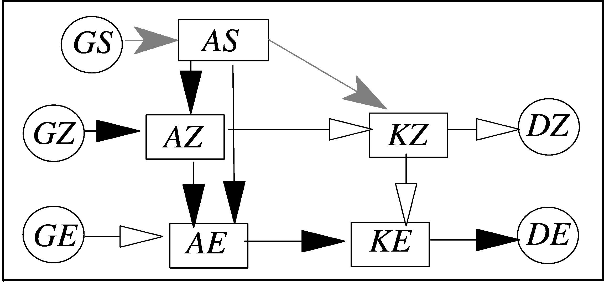
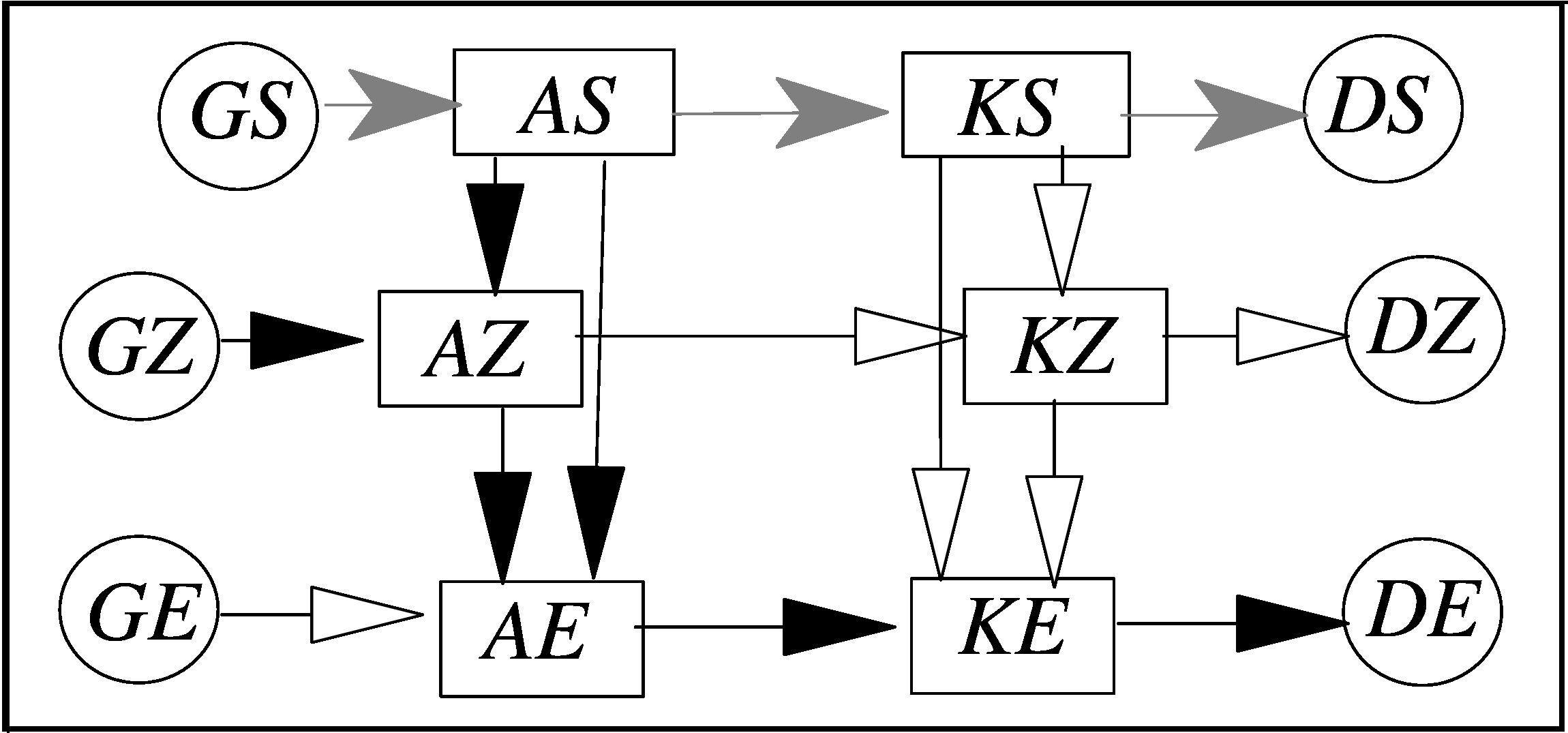
Figure 4: (a) Global and asymmetric $APE$ cycle diagram according to Pearce (1978) ; (b) A possible version for a symmetric and global $AH$ cycle diagram as defined by Marquet (1994). It is close to Pearce’s (1978) diagram except now there are two large-scale kinetic-energy components $KS$ and $KZ$, both connected to $KE$.

The complete limited-area and pressure-level cycle (36) corresponds to Fig. 5(b) where all the terms are depicted. The boundary transport of energy is surrounded by dashed boxes, with a shaded internal Lorenz cycle ($\overline{c_{Z}}$, $\overline{c_{A}}$, $\overline{c_{K}}$, $\overline{c_{E}}$) and with a large external path of energy: $\overline{B(a_{p})}\leftrightarrow\overline{c_{S}}\leftrightarrow\overline{{B(\phi)}_{S}}$.

(a)    The global $A_{h}$-cycle                            (b)    the local $a_{h}$-cycle

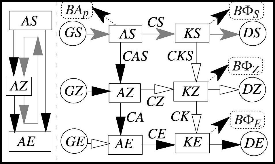
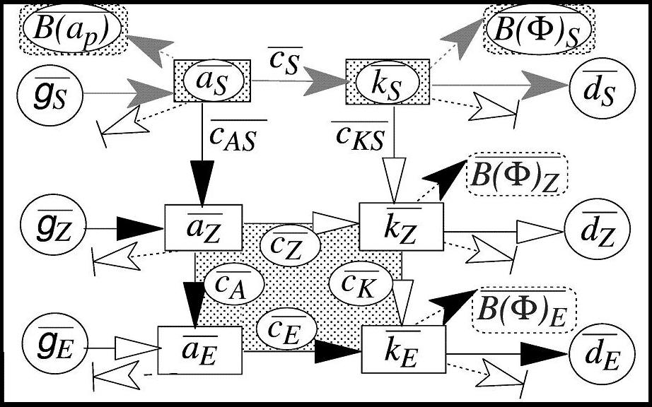
Figure 5: (a) The global and symmetric available-enthalpy cycle diagram as proposed in this paper, including the new connections with potential-energy reservoirs ${B\phi}_{S}$, ${B\phi}_{Z}$ and ${B\phi}_{E}$ (these terms do not disappear because only the sum $\overline{B(\phi)}$ cancels out on global average, not individual components). The left of the diagram shows the modification from Fig. 4(b): a closed inner loop (stippled) is formed by the conversion term $AE\rightarrow AS$ which is subtracted from $AS\rightarrow AE$ and added to the other branches $AS\rightarrow AZ$ and $AZ\rightarrow AE$. A similar modification is done for the path $KS\rightarrow KE$ and $KS\rightarrow KZ\rightarrow KE$. The external path for energy ($AS\leftrightarrow KS$) is now clearly separated from the internal Lorenz cycle ($AZ$, $AE$, $KZ$, $KE$) and, by comparison with Pearce’s formulation, more usual values are obtained for the mathematical expressions of the conversion terms $CA$ and $CK$. (b) The limited area version of (a). The global boundary terms ${B\phi}_{S}$, ${B\phi}_{Z}$ and ${B\phi}_{E}$ in (a) correspond here to the “pressure levels” boundary fluxes $\overline{B(\phi)}_{S}(p)$, $\overline{B(\phi)}_{Z}(p)$ and $\overline{B(\phi)}_{E}(p)$. The six non-labelled outgoing white arrows represent additional boundary fluxes for each of the six energy components (the formulations are given in the first terms on the right-hand sides of (36)).

4.4 Mathematical expressions for all terms.

The six equations in the cycle (36) are expressed in a common form (37) valid for an energy component $e_{X}$. The time derivative $\overline{{\partial}_{t}(e_{X})}$ is equal to boundary flux terms $-\overline{B(e_{X})}$, possibly with further complementary flux $-\overline{B(e_{cX})}$. The conversions terms are $\pm\overline{c_{A}}$ and $\pm\overline{c_{X}}$. The conversion of potential energy into $e_{X}$ is $-\overline{{B(\phi)}_{X}}$, if $e_{X}$ is one of the kinetic energy components. Generation or dissipation terms ($+\;\overline{g_{X}}\;\mbox{or}\;-\overline{d_{X}}$) are present for the case of available-enthalpy or kinetic-energy components, respectively.

$$\overline{{\partial}_{t}(e_{X})}\!\! = \!\!-\;\overline{B(e_{X})}\;-\;\overline{B(e_{cX})}\;\;\;\pm\;\overline{c_{A}}\;\;\;\pm\;\overline{c_{X}}\;\;-\;\overline{{B(\phi)}_{X}}\;\;\;+\left(\;\overline{g_{X}}\;\;\mbox{or}\;-\overline{d_{X}}\;\right).$$ (37)

The general boundary operator $\overline{B(\ldots)}$ is defined using (24). The special case for $\overline{B(a_{p})}=R\>T_{r}\>\overline{B(p)}/p$ is obtained by using $\overline{B(p)}=\overline{\omega}$, to give

$$\overline{B(a_{p})}\!\! = \!\!-\>\frac{R}{p}\;\overline{\omega}\;T_{r}\>.$$ (38)

The first set of conversion terms refers to a transformation of any of the available-enthalpy reservoirs into the corresponding kinetic-energy component with the same status ($S$, $Z$ or $E$). Therefore

$$\overline{c_{S}}\!\! = \!\!-\>\frac{R}{p}\;\overline{\omega}\;\overline{T}\>,\hskip 17.07182pt\overline{c_{Z}}\;=\;-\>\frac{R}{p}\;\overline{{\omega}^{\lambda}_{\varphi}\;{T}^{\lambda}_{\varphi}}\>,\hskip 17.07182pt\overline{c_{E}}\;=\;-\frac{R}{p}\;\overline{{\omega}_{\lambda}\;{T}_{\lambda}}\>,$$ (39)

where the baroclinic conversions $\overline{c_{Z}}$ and $\overline{c_{E}}$ take the classic form. Note that there is no implicit summation over repeated ${\lambda}$ or ${\varphi}$ subscripts or superscripts.

The second set of conversion terms represents energy transformations from one form to another between the three available-enthalpy reservoirs or the three kinetic-energy reservoirs. Thus

$$\overline{c_{AS}} = -\>c_{p}\;\overline{({\omega}^{\>\prime}\;{T}^{\>\prime})}\;\;p^{-{\kappa}}\;\frac{\partial}{\partial\,p}\left\{p^{\kappa}\left(1-\frac{T_{r}}{\overline{T}}\right)\right\}\>,$$ (40)

$$\overline{c_{KS}} = -\left\{\>\overline{({u}^{\>\prime}\;{\omega}^{\>\prime})}\;\;\frac{\partial\,\overline{u}}{\partial\,p}\;+\;\overline{({v}^{\>\prime}\;{\omega}^{\>\prime})}\;\;\frac{\partial\,\overline{v}}{\partial\,p}\>\right\}\>,$$ (41)

$$\overline{c_{A}} = -\>c_{p}\left[\;\overline{{({v}_{\lambda}\>{T}_{\lambda})}^{\lambda}\;\frac{\partial}{\partial\,y}\left(1-\frac{T_{r}}{{T}^{\lambda}}\right)}\;+\;\overline{{({\omega}_{\lambda}\>{T}_{\lambda})}^{\lambda}\>p^{-{\kappa}}\>\frac{\partial}{\partial\,p}\left\{p^{\kappa}\>\left(1-\frac{T_{r}}{{T}^{\lambda}}\right)\right\}}\>\right],$$ (42)

$$\overline{c_{K}} = -\left\{\>\overline{{({u}_{\lambda}{v}_{\lambda})}^{\lambda}\>\frac{\partial\,{u}^{\lambda}}{\partial\,y}}+\overline{{({v}_{\lambda}{v}_{\lambda})}^{\lambda}\>\frac{\partial\,{v}^{\lambda}}{\partial\,y}}+\overline{{({u}_{\lambda}\>{\omega}_{\lambda})}^{\lambda}\>\frac{\partial\,{u}^{\lambda}}{\partial\,p}}+\overline{{({v}_{\lambda}\>{\omega}_{\lambda})}^{\lambda}\>\frac{\partial\,{v}^{\lambda}}{\partial\,p}}\>\right\}.$$ (43)

The baroclinic and barotropic conversions $\overline{c_{A}}$ and $\overline{c_{K}}$ take the classical form.

The boundary terms $\overline{{[B(\phi)]}{}_{\textstyle\eta}}$ with $\eta=S,Z$ or $E$ are the projections of $\overline{B(\phi)}$ onto the three equations for $k_{S}$, $k_{Z}$ and $k_{E}$, respectively. They can be interpreted as conversion terms with the potential energy because $\overline{B(\phi)}$ appears with opposite signs in equations for kinetic and potential energies (31) and (32). They cannot be put in a form $\overline{B[{\phi}_{\textstyle\eta}]}$, i.e. the boundary flux of some ${\phi}_{\textstyle\eta}$ to be determined, as indicated in the local studies of Muench (1965), Brennan and Vincent (1980) or Michaelides (1987). As a consequence $\overline{{[B(\phi)]}{}_{\textstyle\eta}}\neq 0$, with $\eta=S,Z$ or $E$. These terms could not appear in the global approaches of L55 or P78 because the sum of the three projections, i.e. $\overline{B(\phi)}$, has been cancelled out at the beginning of these studies, as a global term equal to zero. However, even in L55 and P78, the terms $\overline{{[B(\phi)]}{}_{\textstyle\eta}}$ is different from $0$ and they should have been present.

The other boundary term $\overline{B(a_{p})}$ with $a_{p}=R\>T_{r}\;\ln(p/p_{r})=R\>T_{r}\;\{\ln(p)-\ln(p_{r})\}$ cancels out if it is integrated over $p_{t}$ and $p_{b}$. It is a consequence of the definition of $p_{r}$ when $\ln(p_{r})$ is equal to the global average of $\ln(p)$.

$$\overline{{B(\phi)}_{S}}\; =\;\overline{u}\;\overline{\left(\frac{\partial\,\phi}{\partial\,x}\right)}\>+\>\overline{v}\;\overline{\left(\frac{\partial\,\phi}{\partial\,y}\right)}\>+\>\overline{\omega}\;\overline{\left(\frac{\partial\,\phi}{\partial\,p}\right)}\hskip 31.29802pt\>=\>\overline{{\bf U}_{h}}\>.\>\overline{{\bf\nabla}_{\!p}\,\phi}\>-\>\frac{R}{p}\;\overline{\omega}\>\overline{T}\>,$$ (44)

$$\overline{{B(\phi)}_{Z}}\; =\;\overline{{u}^{\lambda}_{\varphi}\left(\frac{\partial\,\phi}{\partial\,x}\right){\phantom{\Bigl{(}\Bigr{)}}}^{\lambda}_{\varphi}}\>+\>\overline{{v}^{\lambda}_{\varphi}\left(\frac{\partial\,\phi}{\partial\,y}\right){\phantom{\Bigl{(}\Bigr{)}}}^{\lambda}_{\varphi}}\>+\>\overline{{\omega}^{\lambda}_{\varphi}\left(\frac{\partial\,\phi}{\partial\,p}\right){\phantom{\Bigl{(}\Bigr{)}}}^{\lambda}_{\varphi}}\hskip 1.42262pt\>=\>\overline{{({\bf U}_{h})}^{\lambda}_{\varphi}\>.\>{({\bf\nabla}_{\!p}\,\phi)}^{\lambda}_{\varphi}}\>-\>\frac{R}{p}\;\overline{{\omega}^{\lambda}_{\varphi}\>{T}^{\lambda}_{\varphi}}\>,$$ (45)

$$\overline{{B(\phi)}_{E}}\; =\;\overline{{u}_{\lambda}\left(\frac{\partial\,\phi}{\partial\,x}\right){\phantom{\Bigl{(}\Bigr{)}}}_{\lambda}}\>+\>\overline{{v}_{\lambda}\left(\frac{\partial\,\phi}{\partial\,y}\right){\phantom{\Bigl{(}\Bigr{)}}}_{\lambda}}\>+\>\overline{{\omega}_{\lambda}\left(\frac{\partial\,\phi}{\partial\,p}\right){\phantom{\Bigl{(}\Bigr{)}}}_{\lambda}}\hskip 5.69054pt\>=\>\overline{{({\bf U}_{h})}_{\lambda}\>.\>{({\bf\nabla}_{\!p}\,\phi)}_{\lambda}}\>-\>\frac{R}{p}\;\overline{{\omega}_{\lambda}\>{T}_{\lambda}}\>.$$ (46)

Note that the baroclinic conversions $\overline{c_{S}}$, $\overline{c_{Z}}$ and $\overline{c_{E}}$ appear with the opposite sign in the conversion terms $\overline{c(\phi,k_{X})}=-\overline{{B(\phi)}_{X}}$ for $X=(S,Z,E)$ in Equations (44) to (46). This unexpected property will be discussed in more detail in part II of this paper. The result is that these combinations of terms are equal to the work of the general pressure forces ‘$-{\bf\nabla}_{\!p}(\phi)$’ against the motion and after a projection onto the subset $X=(S,Z,E)$ of components. It gives rise to the equations

$$\overline{c_{S}}\;-\;\overline{{B(\phi)}_{S}} = -\;\overline{{\bf U}_{h}}\>.\>\overline{{\bf\nabla}_{\!p}\phi}\>,$$ (47)

$$\overline{c_{Z}}\;-\;\overline{{B(\phi)}_{Z}} = -\;\overline{{({\bf U}_{h})}^{\lambda}_{\varphi}\>.\>{({\bf\nabla}_{\!p}\phi)}^{\lambda}_{\varphi}}\>,$$ (48)

$$\overline{c_{E}}\;-\;\overline{{B(\phi)}_{E}} = -\;\overline{{({\bf U}_{h})}_{\lambda}\>.\>{({\bf\nabla}_{\!p}\phi)}_{\lambda}}\>.$$ (49)

Finally, the generation and dissipation terms are written as follows

$$\overline{g_{S}}\!\! = \!\!\left(\>1-\frac{T_{r}}{\overline{T}}\>\right)\;\overline{(\>\dot{q}\>)}\hskip 71.13188pt;\hskip 11.38092pt\overline{d_{S}}\;\;\;=\;\;\;-\>\overline{{\bf U}_{h}}\>.\>\overline{{\bf F}_{h}}\>,$$ (50)

$$\overline{g_{Z}}\!\! = \!\!\left(\>\frac{T_{r}}{\overline{T}}\>\right)\;\overline{\left\{\>\left(\>1-\frac{\overline{T}}{{T}^{\lambda}}\>\right)\;\dot{q}\>\right\}}\hskip 19.91684pt;\hskip 11.38092pt\overline{d_{Z}}\;\;\;=\;\;\;-\>\overline{{({\bf U}_{h})}^{\lambda}_{\varphi}}\>.\>\overline{{({\bf F}_{h})}^{\lambda}_{\varphi}}\>,$$ (51)

$$\overline{g_{E}}\!\! = \!\!\overline{\left\{\>\left(\>\frac{T_{r}}{{T}^{\lambda}}\>\right)\;\left(\>1-\frac{{T}^{\lambda}}{T}\>\right)\;\dot{q}\>\right\}}\hskip 17.07182pt;\hskip 11.38092pt\overline{d_{E}}\;\;\;=\;\;\;-\>\overline{{({\bf U}_{h})}_{\lambda}}\>.\>\overline{{({\bf F}_{h})}_{\lambda}}\>.$$ (52)

It is possible to develop the Carnot factors in the generation terms $\overline{g_{Z}}$ and $\overline{g_{E}}$ in order to bring the expressions closer to the corresponding values given in P78: $\overline{\{{T}^{\lambda}_{\varphi}\>{(\dot{q})}^{\lambda}_{\varphi}\}}/T_{r}$ and $\overline{\{{T}_{\lambda}\>{(\dot{q})}_{\lambda}\}}/T_{r}$, respectively. The detailed computations are presented in Appendix-C and the final approximate formulae are given by (C.1) and (C.2). The results

$$\overline{g_{Z}} \approx \overline{\>\left\{\frac{T^{\lambda}_{\varphi}\;{(\dot{q})}^{\lambda}_{\varphi}}{{T}^{\lambda}}\right\}}\>\left(\frac{T_{r}}{\overline{T}}\right)$$

$$\overline{g_{E}} \approx \overline{\left\{\>{\left\{\frac{T_{\lambda}\>{(\dot{q})}_{\lambda}}{T}\right\}}^{\lambda}\>\left(\frac{T_{r}}{{T}^{\lambda}}\right)\right\}}$$

compare relatively well with P78’s expressions.

5 A modified temporal scheme.

An output dataset from the French Arpege model will be used in part II of this paper for post-processed data on $27$ pressure levels at uneven intervals from $10$ to $1000$ hPa. The time derivative and other terms of the cycle (36) will be evaluated with meteorological data, available every $3$ hours. The questions to be addressed are: (i) How to compute the time and spatial differencing? (ii) What are the accuracies of these schemes?

It is usual in papers dealing with energetics to express the time derivative at time $t_{0}$ as a centred finite-difference scheme computed between $t_{(-)}=t_{0}-\Delta t$ and $t_{(+)}=t_{0}+\Delta t$. If (36) is schematically represented by ${\partial}_{t}(Z)=C$ and if the notations $Z^{(+)}$, $Z^{(-)}$ and $C^{(0)}$ are used for values at time $t_{(+)}$, $t_{(-)}$ and $t_{0}$, the usual scheme can be rewritten as

$$\frac{Z^{(+)}-Z^{(-)}}{2\;\Delta t} \approx C^{(0)}\;\;\equiv\;\;\{{\partial}_{t}(Z)\}{}^{(0)}\>.$$ (53)

An objective evaluation of the quality of this scheme will be done using the test functions $Z(t)=\cos(\omega t)$ and $C(t)=-\omega\>\sin(\omega t)$, where $\omega=2\pi/T_{0}$. If $C^{(0)}$ is taken as a reference value, the approximation (53) corresponds to $\{\sin(\pi\ell)\}/(\pi\ell)\approx 1$ for $\ell=\Delta t/{(\Delta t)}_{crit}$ and for a critical time interval equal to ${(\Delta t)}_{crit}=T_{0}/2=\pi/\omega$. In that case, the relative error is equal to ${\varepsilon}_{1}=1-\{\sin(\pi\ell)\}/(\pi\ell)$. Values of ${\varepsilon}_{1}$ are given for $\ell=0.1$ to $\ell=1.4$ in Table 1. This scheme becomes rapidly inaccurate for $\ell>0.3$ or equivalently for $\Delta t>{(\Delta t)}_{crit}/3$, with errors reaching $36$ % or more when $\ell>0.50$.

Table 1: The error functions. Values of ${\varepsilon}_{1}=1-\{\sin(\pi\ell)\}/(\pi\ell)$ and ${\varepsilon}_{2}={\varepsilon}_{1}+\{\cos(\pi\ell)-1\}/3$ for $\ell=\Delta t/{(\Delta t)}_{crit}$ and $\;\>0.1\leq\ell\leq 1.4$

$\ell$ 0.1 0.2 0.3 0.4 0.5 0.6 0.7 0.8 0.9 1.0 1.2 1.4 ${\varepsilon}_{1}$ 0.02 0.06 0.14 0.24 0.36 0.50 0.63 0.77 0.89 1.0 1.16 1.22 ${\varepsilon}_{2}$ 0.00 0.00 0.00 0.01 0.03 0.06 0.10 0.16 0.24 0.33 0.55 0.78

The proposal of this present paper is to write an improved scheme that could manage cases when $\Delta t\approx{(\Delta t)}_{crit}$. The new approach is based on an approximate form of the integral of $C(t)$ in the interval $[t_{(-)};t_{(+)}]$ and on an exact result for the integral of ${\partial}_{t}(Z)$.

$$\int_{t_{(-)}}^{t_{(+)}}\!\!{\partial}_{t}(Z)\>dt\;\equiv\;Z^{(+)}-Z^{(-)}\! = \!\int_{t_{(-)}}^{t_{(+)}}\!\!C\>dt\;\;\;\Longrightarrow$$

$$\frac{1}{2\;\Delta t}\;\int_{t_{(-)}}^{t_{(+)}}\!\!C\>dt\;=\;\frac{Z^{(+)}-Z^{(-)}}{2\;\Delta t}\! \approx \!C^{(0)}\;+\;\frac{\>C^{(+)}-2\,C^{(0)}+C^{(-)}\>}{6}\;.$$ (54)

The integral is computed with an approximation of $C(t)$ around $t=t_{0}$ by a quadratic function of time, defined as $C(t)=a(t-t_{0}){}^{2}+b(t-t_{0})+c$. The three constants are determined by $C(t_{(-)})=C^{(-)}$, $C(t_{0})=C^{(0)}$ and $C(t_{(+)})=C^{(+)}$. They are equal to $a=\{\>C^{(+)}-2\,C^{(0)}+C^{(-)}\>\}/\{2{(\Delta t)}^{2}\}$, $b=\{C^{(+)}-C^{(-)}\}/(2\Delta t)$ and $c=C^{(0)}$. As a result the old scheme (53) is transformed into (54). There is an additional term with weighting factors ($1/6$, $-1/3$, $1/6$). It is zero when $C(t)$ varies linearly with time but can be large in the case of rapid increase or decrease of its change in time.

The objective evaluation for (53) can also be realized for (54) although it leads to the relative error ${\varepsilon}_{2}={\varepsilon}_{1}+\{\cos(\pi\>\ell)-1\}/3$. The corresponding limits of ${\varepsilon}_{1}$ and ${\varepsilon}_{2}$ for small $\ell$ are ${(\pi\>\ell)}^{2}/6$ and ${(\pi\>\ell)}^{4}/180$, respectively. The accuracy is clearly improved and the second-order scheme becomes a fourth-order scheme. Numerical values of ${\varepsilon}_{2}$ are given in Table 1 and it appears that the new scheme is accurate enough up to ${\ell}<0.8$, with an error for $\Delta t\approx{(\Delta t)}_{crit}$ decreasing from $100$ % to $33$ % when replacing (53) by (54).

(a)    Slow advection ($0.7\>L$)                                     (b)    Rapid advection ($1.2\>L$)

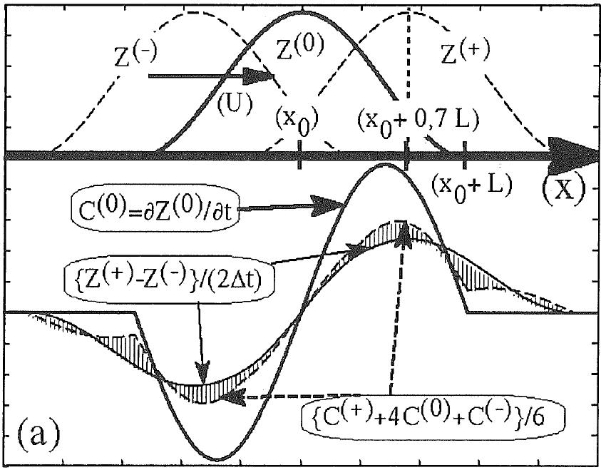
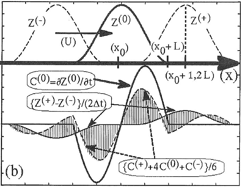
Figure 6: A comparison of accuracy for different numerical schemes to solve ${\partial}_{t}(Z)=C$ for (a) moderate advection and for (b) more rapid advection. The pattern $Z=\cos\{\pi(x-x_{0})/L\}$ where $|x-x_{0}|<L$, is advected by wind $U$ with $x_{0}=U(t-t_{0})$. Length $L$ corresponds the pattern radius. On the upper parts of panels (a) and (b) the curves $Z(x)$ are shown at times $t_{0}-\Delta t$, $t_{0}$ and $t_{0}+\Delta t$. On lower parts the true time derivative $C^{(0)}$ is depicted by a heavy solid line. A thin solid line shows the approximate finite difference (53) and a dashed line shows the new scheme (54). For (a) and (b), the true time derivative $C^{(0)}$ cannot be compared with $\{Z^{(+)}-Z^{(-)})\}/(2\Delta t)$ and (53) is not verified. It is also clear that (54) is valid for (a) because the dashed and thin solid lines are close together, encompassing a small hatched area. But for a rapid advection case (b) the new scheme is no longer valid, as indicated by a hatching area which is too large. It should be mentioned that for small advection (say $\ell=0.3$, not shown) the dashed and thin solid lines cannot be distinguished and (54) is almost exact. Furthermore, for $\ell=0.3$ the solid line is already separated from the others, which means that (53) is rapidly not verified for increasing $\ell$, even when $\Delta t\ll{(\Delta t)}_{crit}$. Symbols are explained in Appendix A.

Improvements in scheme accuracy are confirmed on the basis of the subjective visual analyses presented in Fig. (6). Let us consider the advection by a uniform wind $U$ of a pattern defined by $Z(x,t)=\cos(kx-\omega t+{\alpha}_{0})$, with $k=\pi/L$, $\omega=\pi U/L$ and ${\alpha}_{0}=\pi Ut_{0}/L$. The accuracies of the old and new schemes (53) and (54) can be evaluated by visual comparisons of the different lines depicted on the lower parts of Fig.(6)(a) and (b), with $\ell\approx 0.7$ for Fig.(6)(a) and $\ell\approx 1.2$ for Fig.(6)(b).

It appears that the old scheme is not verified for any of the two cases because the heavy lines for $C^{(0)}$ are clearly separated from the other two. The accuracy of the new scheme can be appreciated by the small hatched area. If the new scheme is valid for the moderate advection scheme in Fig.(6)(a), it is no longer valid in Fig.(6)(b) when $\Delta t\approx 1.2{(\Delta t)}_{crit}$. So, the subjective limits are equivalent to the objective ones and in order to ensure an accuracy better than $16$ % the time interval must verify $\ell<0.3$ for (53) and $\ell<0.8$ for (54).

The critical time interval can be small in the case of real small-scale meteorological features like frontal waves or mobile troughs. For the example, presented in Figure (3) of Michaelides (1987), the observation of the successive panels indicate a radius of about $10\,{}^{\circ}$ for the depression and a zonal advection of about $10\,{}^{\circ}$ (day)^-1. As a consequence, the critical time interval is equal to $1$ day and the limits required for relevant applications of (53) or (54) are respectively equal to $7$ h and $19$ h.

The new scheme can be interpreted as a ‘moving average’ approach centred on $t_{0}$, with a window of $\pm\Delta t$. It is when all terms in (36) are computed with (54) as moving averages that the dissipation and generation terms can be derived as moving average residuals. Large values of dissipation and generation terms, described in previous papers dealing with local energetics, are perhaps partly due to the imbalance in (53) and to values of $\Delta t$ close to or above ${(\Delta t)}_{crit}$.

6 Discussion of $T_{r}$, $p_{r}$ and the reference state.

The choice of prescribed and constant values for $T_{r}$ and $p_{r}$ is often open to criticism. It appears to be a problem for the use of more complex reference states (non-uniform, non-stationary or without zonal-mean symmetry). However, the possibility of choosing more complex “reference states” does exist with the present available-enthalpy approach. There is a real possibility of defining a less academic and more realistic basic state.

Even if a constant temperature $T_{r}$ is used as in P78 to define an isothermal “thermodynamic reference atmosphere”, in Pearce’s and this paper, the real “reference meteorological state” must be thought of in terms of the additional isobaric and zonally averaged quantities $\overline{T}(p,t)$ and ${T}^{\lambda}(\varphi,p,t)$. These are time-dependent states of the atmosphere, based on real meteorological datasets.

Another isothermal reference state $T_{0}=\>$constant have been used by Andrews (1981) to define the potential energy for a perfect gas by

$$\Pi\;=\;{\Pi}_{1}(p/p_{0})\>+\>{\Pi}_{2}(\theta/{\theta}_{0})\>,$$

where the two parts ${\Pi}_{1}$ and ${\Pi}_{2}$ are local and positive-definite everywhere. The second part can be written as

$${\Pi}_{2}(\eta)\;=\;c_{p}\;T_{0}\;h(\eta)\>,$$

with $h(\eta)=\exp(\eta)-1-\eta$ and $\eta=\ln(\theta/{\theta}_{0})$. It is thus equal to

$${\Pi}_{2}(X)\;=\;c_{p}\;T_{0}\;{\cal F}(X)\>,$$

where $X=\theta/{\theta}_{0}-1$ and the function ${\cal F}(X)=X-\ln(1+X)$ is the same function used in (6) to define $a_{T}=c_{p}\>T_{r}\;{\cal F}(T/T_{r}-1)$.

The reference values $T_{r}$ and $p_{r}$ are introduced in order to isolate the pressure component $a_{p}=R\;T_{r}\>\ln(p/p_{r})$ and to define the “zero-order” quadratic function $a_{T}=c_{p}\>T_{r}\>{\cal F}\{(T-T_{r})/T_{r}\}$. The separating property (7) has then been used to successively insert the first- and second-order departure terms of Lorenz: $T_{1}={T}^{\lambda}_{\varphi}$ and $T_{2}={T}_{\lambda}$. The same separating property can easily be used to deal with other “eddy” and “mean” energetic investigations, with more complex definitions for the average terms (e.g. for temporal or spatial moving averages of the flow, with possible tilted features and complex geometry over the limited area domain).

Actually the choice of $T_{r}$ and $p_{r}$ is not a central point for atmospheric purposes. Other developments could be pursued in the future with other possible definitions for $T_{1}$ and $T_{2}$ to be inserted between the same $T$ and $T_{r}$. A new problem would, however, appear in that case since the algebra in Appendix B would not be easy to use, making the derivation of the energy cycle (36) very difficult in most cases. Here lies the success of Lorenz’s separation into ${T}^{\lambda}_{\varphi}$ and ${T}_{\lambda}$, even when it is applied to the available-enthalpy function and to limited-area domains.

7 Conclusions.

The specific available enthalpy function (3) has been used to derive the complete energy cycle (36). It can be applied to any pressure level of any limited-area atmospheric domain. It is an exact cycle with $A3+K3$ components corresponding to Fig. 5 (b). There are no approximations and no missing terms. The demonstration of this affirmation will be obtained in part II of this paper when the generation and the dissipation terms will be computed as residuals of Eqs.(36) using the modified temporal scheme (54). Logically these residuals should be small in the case of adiabatic studies of idealized simulations of baroclinic waves, whereas they were very large in previous studies where some terms of (36) were missing.

The approach followed in this paper is similar to some extent to L55 and P78 in that the basic states ${T}^{\lambda}$, ${u}^{\lambda}$ and ${v}^{\lambda}$ are zonally symmetric. The eddy and zonally symmetric components $\overline{a_{E}}$ and $\overline{a_{Z}}$ are almost the same as in L55, but the averaged stability $\overline{\sigma}$ is disregarded and replaced, as in P78, by an additional static stability component $a_{S}$. The kinetic components are defined similarly by $\overline{k_{E}}$, $\overline{k_{Z}}$ and $k_{S}$, for the sake of symmetry with the partitioning of the available enthalpy components.

The global and local (“pressure level”) versions of the available-enthalpy cycle represented by Fig. 5 (a) and (b) differ only by some boundary fluxes, as it should be. The transformations required to go from Lorenz cycle to the local available-enthalpy cycle are illustrated by considering the series of Figs.1, 4 (b), 5 (a) and 5 (b).

In the new cycle, the baroclinic and barotropic conversion terms $\overline{c_{E}}$ and $\overline{c_{Z}}$ in (39) and (43) take their classical form. However, they are obtained by the usual transformation of horizontal wind $-{\bf U}_{h}\>.\>{\bf\nabla}_{\!p}\>(\phi)$ into $-\>B(\phi)-R\>\omega\>T/{p}$, where the second term uses the vertical wind. This manipulation leads to cancellation of the boundary term $-\>B(\phi)$ on a global scale which simplifies the study of L55.

This, though, is no longer true for the local study presented here. It could be more advantageous to keep the initial formulation $-{\bf U}_{h}\>.\>{\bf\nabla}_{\!p}\>(\phi)$ when budgets of kinetic-energy components are considered, or equivalently $f\>{\bf k}\>.\left({\bf U}_{g}\times{\bf U}_{a}\right)$, where ${\bf U}_{g}$ and ${\bf U}_{a}$ are the geostrophic and ageostrophic winds, respectively. The main problem is that the classical baroclinic conversion $-R\>\overline{{\omega}_{\lambda}\>{T}_{\lambda}}/p$ is contained in both $\overline{c_{E}}$ and in $-\overline{{B(\phi)}_{E}}$ with the opposite sign. As a consequence, it does not contribute to any change in $\overline{k_{E}}$ and a careful comparison of the two formulations, using ageostrophic or vertical winds, is thus necessary. This will be done in part II, based on applications to idealize adiabatic and diabatic simulations.

Acknowledgements.

The author is most grateful to S. Malardel for his initial support regarding the applications of available-enthalpy energetics to idealized simulations. I also thank R. Clark and the two referees who suggested many clarifications and modifications to the manuscript.

Appendix A. Basic notation.  

$a$, $A$	Local and global available enthalpy (Pearce, 1978).
$a_{h}$, $A_{h}$	Local specific and global available enthalpy.
$a_{T}$, $A_{T}$	Local specific and global temperature-component of $a_{h}$ and $A_{h}$.
$a_{p}$, $A_{p}$	Local specific and global pressure-component of $a_{h}$ and $A_{h}$.
$\overline{a_{S}}$, $\overline{a_{Z}}$, $\overline{a_{E}}$	Basic available-enthalpy components.
$\overline{a_{cS}}$, $\overline{a_{cZ}}$	Complementary available-enthalpy components.
$a_{e1}$, $a_{e2}$	Local specific values for two available-energies.
APE	Global available potential energies (Lorenz, 1955)
$\overline{B(\ldots)}$	Boundary flux terms for all energy components
$\overline{{B(\phi)}_{S}}$, $\overline{{B(\phi)}_{Z}}$, $\overline{{B(\phi)}_{E}}$	Potential-energy special conversion terms
$B$, $E$, $S$, $Z$	Subscripts for baroclinicity, eddy, static-stability and zonal components
$BA_{h}$, $BK$, $BA_{p}$, $B(\phi)$	Global boundary flux terms
$\overline{c_{A}}$, $\overline{c_{Z}}$, $\overline{c_{E}}$, $\overline{c_{K}}$	Basic conversions
$\overline{c_{S}}$, $\overline{c_{AS}}$, $\overline{c_{KS}}$	Other basic conversions involving $\overline{a_{S}}$
$\overline{c_{a}}$	Ageostrophic conversion (Part II)
$\overline{(c_{ag})_{S}}$, $\overline{(c_{ag})_{Z}}$, $\overline{(c_{ag})_{E}}$	Ageostrophic conversions (Part II)
$c_{p}$	Specific heat at constant pressure for dry air
$d$, $D$	Local and global dissipation terms
$\overline{d_{S}}$, $\overline{d_{Z}}$, $\overline{d_{E}}$	Dissipation terms
$e_{i}$, ${(e_{i})}_{r}$	Local specific values for internal energy, reference value of $e_{i}$
$e_{k}$	Local specific values for kinetic energy
$e_{p}=\phi$	Local specific values for potential energy
$E_{i}$	Global internal energy
$E_{p}$	Global potential energy
$f$, $f^{\ast}$	Coriolis and pseudo Coriolis factor
${\bf F}_{h}$, $(F_{h})_{x}$, $(F_{h})_{y}$	Frictional force and its horizontal components
$\cal{F}$	An exergy (quadratic) function
$\cal{G}$	An exergy (quadratic) function
$g$, $G$	Local and global generation terms
$\overline{g_{S}}$, $\overline{g_{Z}}$, $\overline{g_{E}}$	Generation terms
$h$, $h_{r}$, $h_{00}$	Local specific enthalpy, reference and standard values of $h$
$H$	Global enthalpy
$H_{pbl}$	Scale height of the Planetary Boundary Layer (Part II)
${\bf k}$	Vertical unit vector
$\overline{k_{S}}$, $\overline{k_{Z}}$, $\overline{k_{E}}$	Pressure-level average kinetic-energy components of $e_{k}$
$\overline{K_{S}}$, $\overline{K_{Z}}$, $\overline{K_{E}}$	Global kinetic-energy components (KS, KZ and KE in Figures)
$\overline{k_{cS}}$, $\overline{k_{cZ}}$	Complementary kinetic-energy components.
$K$	Global kinetic energy
$L$	Mixing length for the vertical dissipation scheme (Part II)
$p$, $p_{r}$, $p_{00}$	Local pressure, reference and standard values of $p$
$p_{t}$, $p_{b}$	Pressure at top and bottom of atmosphere
$\dot{q}$	Diabatic heating
$R$	Gas constant
${\cal R}$	Earth radius
$s$, $s_{r}$, $s_{00}$	Local specific entropy, reference and standard values of $s$
$S$	Global entropy
$T$, $T_{r}$, $T_{00}$	Local temperature, reference and standard values of $T$
$T_{1}$, $T_{2}$	Two reference temperatures used in section 6 (Part I)
“$T_{0}\Sigma$”	Global static entropic energy
TPE	Global total potential energies (Lorenz, 1955)
${\bf U}_{h}=(u,v)$	Horizontal wind speed and its components
${\bf U}_{g}=(u_{g},v_{g})$	Geostrophic horizontal wind and its components
${\bf U}_{a}=(u_{a},v_{a})$	Ageostrophic horizontal wind and its components
$V_{a}$, $V_{b}$	Geostrophic and ageostrophic wind in complex notation (Part II)
$X$, $X_{1}$, $X_{2}$	Dummy arguments of $\cal{F}$ and $\cal{G}$ exergy (quadratic) functions
$z$, $z_{b}$	Height above surface and bottom of atmosphere (Part II)
($a$, $b$, $c$)	Coefficients used in section 5 (Part I)
$\ell$	Dummy value used in section 5 (Part I)
${\alpha}$, ${\alpha}_{r}$	Inverse of density, reference value of ${\alpha}$
$\eta$	A dummy variable
${\varepsilon}_{1}$, ${\varepsilon}_{2}$	Two error functions
$\phi=g\>z$	Local specific potential energy ($g$ is the acceleration due to gravity)
$\lambda$	Longitude
$\varphi$	Latitude
$\Lambda$	A scale height (Part II)
$\overline{\sigma}\,(p)$	Average static stability on a pressure level (Lorenz, 1955)
$\omega=d/dt(p)$	Vertical velocity in pressure coordinates
$\Omega$	Angular velocity of the Earth
$\kappa=R/c_{p}$	A non-dimensional number
$\theta$	A general surface angle (Part II)
${\bf\nabla}_{\!p}(\phi)$	Pressure force
$[{\bf\nabla}_{\!p}(\phi)]_{x}$, $[{\bf\nabla}_{\!p}(\phi)]_{y}$	Horizontal components of pressure force
$d/dt(\ldots)$	${\partial}/{\partial t}(\ldots)+{{\bf U}_{h}}\>.\>{\bf\nabla}_{\!p}(\ldots)+\omega\>{\partial}/{\partial p}(\ldots)$ : the material derivative
${\cal V}_{T}$	A non-dimensional number
$\psi$, $\Psi$	Two dummy variables

The notation used in this paper is adapted from Reiter (1969). Let us consider any pressure level within a limited-area domain limited by south and north latitudes ${\varphi}_{s}$ and ${\varphi}_{n}$ and by east and west longitudes ${\lambda}_{e}$ and ${\lambda}_{w}$. Horizontal averaging operators ${\psi}^{\varphi}(\lambda,p)$ and ${\psi}^{\lambda}(\varphi,p)$ will be indicated by superscripts, they are defined for any local scalar ${\psi}(\lambda,\varphi,p)$ by

$${\psi}^{\varphi}\> = \>\frac{1}{\sin({\varphi}_{n})-\sin({\varphi}_{s})}\;\int_{{\varphi}_{s}}^{{\varphi}_{n}}\!{\psi}\>\cos(\varphi)\;d\varphi\>,$$

$${\psi}^{\lambda}\> = \>\frac{1}{{\lambda}_{e}-{\lambda}_{w}}\;\int_{{\lambda}_{w}}^{{\lambda}_{e}}\!{\psi}\;d\lambda\>.$$

The average and departure terms are defined by

$$\overline{{\psi}} = ({{\psi}}^{\varphi}){}^{\lambda}\>=\>({{\psi}}^{\lambda}){}^{\varphi}\>=\>{{\psi}}^{\lambda}{}^{\varphi}\>,$$ (A.1)

$${\psi}_{\lambda} = {\psi}-{{\psi}}^{\lambda}\;\;;\;\;{\psi}^{\lambda}_{\varphi}\>=\>{\psi}^{\lambda}-{{\psi}}^{\lambda}{}^{\varphi}\>=\>{\psi}^{\lambda}-\overline{{\psi}}\>,$$ (A.2)

$${\psi}^{\>\prime} = {\psi}-\overline{{\psi}}\>=\>{\psi}^{\lambda}_{\varphi}+{\psi}_{\lambda}\>,$$ (A.3)

where departure terms are indicated by subscripts.

The global value ${\Psi}$ is defined from any local value ${\psi}(t,\lambda,\varphi,p)$ by

$${\Psi}\>=\int_{p_{t}}^{p_{b}}\overline{{\psi}}\;\;\frac{dp}{g}\>,$$

where $p_{t}$ and $p_{b}$ are the pressure at the bottom and top of the atmosphere. The horizontal and time derivatives at constant pressure and the vertical derivative are:

$${\partial}_{x} = \frac{\partial}{\partial x}\>(\ldots)\>=\>\frac{1}{{\cal R}\cos(\varphi)}\>{\left[\frac{\partial}{\partial\lambda}\>(\ldots)\right]}_{(t,{\varphi},p)}\>,$$

$${\partial}_{y} = \frac{\partial}{\partial y}\>(\ldots)\>=\>\frac{1}{\cal R}\>\>{\left[\frac{\partial}{\partial\varphi}\>(\ldots)\right]}_{(t,{\lambda},p)}\>,$$

$${\partial}_{t} = \frac{\partial}{\partial t}\>(\ldots)\>=\>\>{\left[\frac{\partial}{\partial t}\>(\ldots)\right]}_{({\lambda},{\varphi},p)}\>,$$

$${\partial}_{p} = \frac{\partial}{\partial p}\>(\ldots)\>=\>-\>\frac{R\>T}{g\>p}\>{\left[\frac{\partial}{\partial z}\>(\ldots)\right]}_{(t,{\lambda},{\varphi})}\>.$$

Appendix B. The local available enthalpy cycle.  

The first stages of the computations leading to the available enthalpy cycle (36) will be described, though only for the component $a_{Z}$. Similar methods can be applied to the five other components. The first step is to compute the derivation at constant pressure with respect to any $\eta$ variable ($\eta=t$, $\lambda$, $\varphi$), or with respect to pressure if $\eta=p$. The result is

$$\overline{{\partial}_{\eta}(a_{Z})}\> = \>\overline{{\partial}_{\eta}\left\{\>c_{p}\>T_{r}\>{\cal F}\!\left(\frac{T^{\lambda}_{\varphi}}{\overline{T}}\right)\>\right\}}$$

$$= \>c_{p}\>\left(\frac{T_{r}}{\overline{T}}\right)\>\overline{\left\{\>\>\left(\frac{\overline{T}}{T^{\lambda}}\right)\>{T^{\lambda}_{\varphi}}\;{\partial}_{\eta}(T^{\lambda})-{\partial}_{\eta}(\overline{T})\>\right\}}\>.$$ (B.1)

The time derivative is transformed using the commutating properties between ${\partial}_{t}(...)$ and ${(...)}^{\lambda}$, to give

$$\overline{{\partial}_{t}(a_{Z})} = c_{p}\>\left(\frac{T_{r}}{\overline{T}}\right)\>\overline{\left\{\>\>\left(\frac{\overline{T}}{T^{\lambda}}\right)\>{T^{\lambda}_{\varphi}}\;{({\partial}_{t}T)}^{\lambda}-\overline{({\partial}_{t}T)}\>\right\}}\>.$$ (B.2)

The boundary terms are obtained from (B.1) for $a_{Z}$ and with the equivalent equation for $a_{cZ}$ given by (16). The results can be rearranged into

$$\overline{B(a_{Z})} = c_{p}\>\left(\frac{T_{r}}{\overline{T}}\right)\>\overline{\left\{\>\>\left(\frac{\overline{T}}{T^{\lambda}}\right)\>{T^{\lambda}_{\varphi}}\;{B({T}^{\lambda})}-{B(\overline{T})}\>\right\}}\;,$$ (B.3)

$$\overline{B(a_{cZ})} = c_{p}\>\left(\frac{T_{r}}{\overline{T}}\right)\>\overline{\left[\left(\frac{T^{\lambda}_{\varphi}}{T^{\lambda}}\right)\>{B({T})}-\left(\frac{T_{\lambda}}{\overline{T}}\right)\>{B(\overline{T})}+\left\{\frac{T\>{\overline{T}}}{{(T^{\lambda})}^{2}}-1\right\}\>B(T^{\lambda})\right]}\;.$$ (B.4)

Equation (30) in then used to express $\overline{{\partial}_{t}(T)}$ in (B.2) and, after long and exact manipulations, the quantity $\overline{{\partial}_{t}(a_{Z})}+\overline{B(a_{Z}+a_{cZ})}$, which is equal to (B.2)$+$ (B.3)$+$ (B.4), is found to be equal to the sum $\>+\>\overline{c_{AS}}-\overline{c_{Z}}-\overline{c_{A}}+\overline{g_{Z}}$, as indicated in (36), without approximations or cancelled terms.

Appendix C. Approximation formulas for $g_{Z}$ and $g_{E}$.  

Starting from Eqs. (51) and (52), the diabatic heating $(\dot{q})$ is separated differently for $\overline{g_{Z}}$ and $\overline{g_{E}}$. It is found, with the use of ${[T^{\lambda}_{\varphi}\>{(\dot{q})}_{\lambda}]}^{\lambda}=0$ for $\overline{g_{Z}}$, that

$$\frac{\overline{g_{Z}}}{T_{r}}\> = \>\overline{\left[\>\left(\frac{T^{\lambda}_{\varphi}}{\overline{T}}\right)\;\left(\frac{\>\overline{(\dot{q})}+{(\dot{q})}^{\lambda}_{\varphi}+{(\dot{q})}_{\lambda}}{{T}^{\lambda}}\>\right)\right]}\;,$$

$$= \>\overline{\left(\frac{T^{\lambda}_{\varphi}}{T^{\lambda}}\right)}\;\;\frac{\overline{(\dot{q})}}{\overline{T}}\>+\>\overline{\left[\;\>\frac{T^{\lambda}_{\varphi}}{{T}^{\lambda}}\;\;\frac{{(\dot{q})}^{\lambda}_{\varphi}}{\overline{T}}\;\right]}\>,$$

and

$$\frac{\overline{g_{E}}}{T_{r}}\> = \>\overline{\left[\>\left(\frac{T_{\lambda}}{T}\right)\;\left(\>\frac{{(\dot{q})}^{\lambda}+{(\dot{q})}_{\lambda}}{{T}^{\lambda}}\right)\right]}\>,$$

$$= \>\overline{\left[\>{\left(\frac{T_{\lambda}}{T}\right)}^{\lambda}\;\frac{{(\dot{q})}^{\lambda}}{{T}^{\lambda}}\right]}\>+\>\overline{\left[\>\left(\frac{T_{\lambda}}{{T}^{\lambda}}\right){\left(\frac{{(\dot{q})}_{\lambda}}{T}\right)}^{\lambda}\right]}\>.$$

The last terms of these equations, say $\overline{\>[T^{\lambda}_{\varphi}\;{(\dot{q})}^{\lambda}_{\varphi}/{T}^{\lambda}]}$ and $\overline{\{\>{[T_{\lambda}\>{(\dot{q})}_{\lambda}/T]}^{\lambda}/{T}^{\lambda}\}}$, are close to the definition given in P78 and it can be demonstrated that the first terms $\overline{(T^{\lambda}_{\varphi}/T^{\lambda})}\;[\overline{(\dot{q})}/\overline{T}]$ and $\overline{\{\>{(T_{\lambda}/T)}^{\lambda}\;[{(\dot{q})}^{\lambda}/{T}^{\lambda}]\}}$ are one order of magnitude smaller. Indeed, it appears that absolute values of the first non dimensional terms $A=\overline{(T^{\lambda}_{\varphi}/T^{\lambda})}$ and $B={(T_{\lambda}/T)}{}^{\lambda}$ are small when compared to unity. The demonstration starts with $A=1-\overline{(\overline{T}/T^{\lambda})}$ and $B=1-{(T^{\lambda}/T)}{}^{\lambda}$. From Eq. (A.2), the use of $T^{\lambda}=T^{\lambda}_{\varphi}+\overline{T}$ in $A$ and of $T=T^{\lambda}+T_{\lambda}$ in $B$ lead to

$$A=1-\overline{\left(\frac{1}{1+T^{\lambda}_{\varphi}/\overline{T}}\right)}\;\;\;\;\;\mbox{and}\;\;\;\;B=1-\left(\frac{1}{1+T_{\lambda}/T^{\lambda}}\right)^{\lambda}\>.$$

For small $|x|$, $1/(1+x)\approx 1-x+x^{2}$ and the limits for small $|T^{\lambda}_{\varphi}/\overline{T}|$ and $|T_{\lambda}/T^{\lambda}|$ are $A\approx-\overline{\{{(T^{\lambda}_{\varphi}/\overline{T})}{}^{2}\}}$ and $B\approx-{\{{(T_{\lambda}/T^{\lambda})}{}^{2}\}}{}^{\lambda}$. The first order term “$-x$” cancels out in both cases because $\overline{(T^{\lambda}_{\varphi})}={(T_{\lambda})}^{\lambda}=0$. As a consequence, the terms $\overline{\{\>{(T_{\lambda}/T)}^{\lambda}\;[{(\dot{q})}^{\lambda}/{T}^{\lambda}]\}}$ and $\overline{(T^{\lambda}_{\varphi}/T^{\lambda})}\;[\overline{(\dot{q})}/\overline{T}]$ in the expressions above are small and the following approximations (C.1) and (C.2) are close to the results obtained in P78, namely $\overline{\{{T}^{\lambda}_{\varphi}\>{(\dot{q})}^{\lambda}_{\varphi}\}}/T_{r}$ and $\overline{\{{T}_{\lambda}\>{(\dot{q})}_{\lambda}\}}/T_{r}$, respectively. The local available-enthalpy versions of generations terms thus become

$$\overline{g_{Z}}\!\! \approx \!\!\overline{\>\left\{\frac{T^{\lambda}_{\varphi}\;{(\dot{q})}^{\lambda}_{\varphi}}{{T}^{\lambda}}\right\}}\>\left(\frac{T_{r}}{\overline{T}}\right)\>,$$ (C.1)

$$\overline{g_{E}}\!\! \approx \!\!\overline{\left\{\>{\left\{\frac{T_{\lambda}\>{(\dot{q})}_{\lambda}}{T}\right\}}^{\lambda}\>\left(\frac{T_{r}}{{T}^{\lambda}}\right)\right\}}\>.$$ (C.2)

They correspond to equations mentioned at the end of section 4.

References.

$\bullet$ Andrews, D. 1981. A note on potential energy in a stratified compressible fluid. J. Fluid Mech., 107, p.227–236.

$\bullet$ Bernard-Bouissières, I., Cadiou, M., Muzellec, A., Vincent, Ch. 1991. Cycles énergétiques. Internal report of the French School of Meteorology.

$\bullet$ Brennan, F. E. and Vincent, D. G. 1980. Zonal and eddy components of the synoptic-scale energy budget during intensification of hurricane Carmen (1974). Mon. Weather Rev. 108, p.954–965.

$\bullet$ Carnot, N, L, S. 1824. Réflexions sur la puissance motrice du feu, et sur les machines propres à développer cette puissance. See the account of Carnot’s theory written by W. Thomson (1849) in the Trans. Roy. Soc. Edinb. 16, p.541–574. An English translation by R. H. Thurston of the version published in the “Anales scientifique de l’École Normale Supérieure” (ii. series, t.1, 1872) is available in the url: http://www3.nd.edu/~powers/ame.20231/carnot1897.pdf (Wiley & Sons, 1897, digitized by Google)

$\bullet$ Clausius, R. 1865. Über verschiedene für die Anwendung bequeme Formen der Hauptgleichungen der mechanischen Wärmetheorie. (On Different Forms of the Fundamental Equations of the Mechanical Theory of Heat). Ann. der Phys. und Chem. 125, p.353-400.

$\bullet$ Courtier, J. A., Freydier, C., Geleyn, J.F., Rabier, F. and Rochas, M. 1991. The Arpège project at Météo-France. ECMWF Seminar Proceedings., Reading, 9-13 Sept. 1991, Volume II, p.193–231.

$\bullet$ Dutton, J. A. 1973. The global thermodynamics of atmospheric motion. Tellus. 25, (2), p.89–110.

$\bullet$ Engel, F., Petit, B., Pontaud, M. 1992. Un cycles énergétiques local associé au modèle non-hydrostatique de COME : applications à une onde d’est. Internal report of the French School of Meteorology.

$\bullet$ Gibbs, J. W. 1873. A method of geometrical representation of the thermodynamic properties of substance by means of surfaces. Trans. Connecticut Acad. II: p.382–404. (Pp 33–54 in Vol. 1 of The collected works of J. W. Gibbs, 1928. Longmans Green and Co.)

$\bullet$ Karlsson, S. 1990. Energy, Entropy and Exergy in the atmosphere. Thesis of the Institute of Physical Resource Theory. Chalmers University of Technology. Göteborg, Sweden.

$\bullet$ Kasahara, A. 1974. Various vertical coordinate systems used for numerical weather prediction. Mon. Weather Rev. 102, p.509–522.

$\bullet$ Kucharski, F. 1997. On the concept of exergy and available potential energy. Q. J. R. Meteorol. Soc. 123, p.2141–2156.

$\bullet$ Livezey, R. E. and Dutton, J. A. 1976. The entropic energy of geophysical fluid systems. Tellus. 28, (2), p.138–157.

$\bullet$ Lorenz, E. N. 1955. Available potential energy and the maintenance of the general circulation. Tellus. 7, (2), p.157–167.

$\bullet$ McHall,  Y. L., 1990. Available potential energy in the atmospheres. Meteorol. Atmos. Phys., 42, p.39–55.

$\bullet$ Margules, M. 1903-05. On the energy of storms. Smithsonian Miscellaneous collections, 51, 4, 533–595, 1910. (Translation by C. Abbe from the appendix to the annual volume for 1903 of the Imperial Central Institute for Meteorology, Vienna, 1905. ‘Über die energie der stürme’. Jahrb. Zentralantst. Meteorol., 40, p.1–26, 1903).

$\bullet$ Marquet P. 1991. On the concept of exergy and available enthalpy: application to atmospheric energetics. Q. J. R. Meteorol. Soc. 117: p.449–475. http://arxiv.org/abs/1402.4610. arXiv:1402.4610 [ao-ph]

$\bullet$ Marquet, P. 1994. Applications du concept d’exergie à l’énergétique de l’atmosphère. Les notions d’enthalpie utilisables sèche et humide. PhD-thesis of the Paul Sabatier University. Toulouse, France.

$\bullet$ Marquet, P. 1995. On the concept of pseudo-energy of T. G. Shepherd. Q. J. R. Meteorol. Soc. 121: p.455–459. http://arxiv.org/abs/1402.5637. arXiv:1402.5637 [ao-ph]

$\bullet$ Marquet, P. 2001. The available enthalpy cycle. Applications to idealized baroclinic waves.. Note de centre du CNRM. Number 76. Toulouse, France.

$\bullet$ Marquet P. 2003a. The available enthalpy cycle. Part I : Introduction and basic equations. Q. J. R. Meteorol. Soc., 129, (593), p.2445–2466.

$\bullet$ Marquet P. 2003b. The available enthalpy cycle. Part II : Applications to idealized baroclinic waves. Q. J. R. Meteorol. Soc., 129, (593), p.2467–2494.

$\bullet$ Maxwell, J. C. 1871. Theory of Heat. References are made in the text to next editions of this book. Longmans, Green and Co. London.

$\bullet$ Michaelides, S. C. 1987. Limited area energetics of Genoa cyclogenesis. Mon. Weather Rev. 115, p.13–26.

$\bullet$ Muench, H. S. 1965. On the dynamics of the wintertime stratosphere circulation. J. Atmos. Sci. 22, p.349-360.

$\bullet$ Normand, Sir C. 1946. Energy in the atmosphere. Q. J. R. Meteorol. Soc., 72, p.145–167.

$\bullet$ Pearce, R. P. 1978. On the concept of available potential energy. Q. J. R. Meteorol. Soc. 104, p.737–755.

$\bullet$ Pichler, H. 1977. Die bilanzgleichung für die statischer entropische Energie der Atmosphäre. Arch. Met. Geoph. Biokl., Ser.A, 26, p.341–347.

$\bullet$ Reiter, E. R. 1969. Mean and eddy motions in the atmosphere. Mon. Weather Rev., 97, p.200–204.

$\bullet$ Saltzman, B. and Fleischer, A. 1960. The modes of release of available potential energy in the atmosphere. J. Geophys. Res. 65, (4), p.1215–1222.

$\bullet$ Shepherd, T. G. 1993 A unified theory of available potential energy. Atmosphere-Ocean., 31, p.1–26.

$\bullet$ Thomson, W. 1849. An account of Carnot’s theory of the “Motive Power of Heat”, with numerical results deduced from Regnault’s experiments on steam. Trans. Roy. Soc. Edinb. 16, Part 5, p.541–574.

$\bullet$ Thomson, W. 1853. On the restoration of mechanical energy from an unequally heated space. Phil. Mag. 5, 30, 4e series, p.102–105.

$\bullet$ Thomson, W. 1879. On thermodynamic motivity. Phil. Mag. 7, 44, 5e series, p.346–352.