Solving fractional Schrödinger-type spectral problems: Cauchy oscillator and Cauchy well

Abstract

This paper is a direct offspring of Ref. GS where basic tenets of the nonlocally induced random and quantum dynamics were analyzed. A number of mentions was maid with respect to various inconsistencies and faulty statements omnipresent in the literature devoted to so-called fractional quantum mechanics spectral problems. Presently, we give a decisive computer-assisted proof, for an exemplary finite and ultimately infinite Cauchy well problem, that spectral solutions proposed so far were plainly wrong. As a constructive input, we provide an explicit spectral solution of the finite Cauchy well. The infinite well emerges as a limiting case in a sequence of deepening finite wells. The employed numerical methodology (algorithm based on the Strang splitting method) has been tested for an exemplary Cauchy oscillator problem, whose analytic solution is available. An impact of the inherent spatial nonlocality of motion generators upon computer-assisted outcomes (potentially defective, in view of various cutoffs), i.e. detailed eigenvalues and shapes of eigenfunctions, has been analyzed.

I Introduction

A fully fledged theory of quantum dynamical patterns of behavior that are nonlocally induced has been carefully analyzed in Ref. GS . The pertinent motion scenario stems from generalizing the standard Laplacian-based framework of the Schrödinger picture quantum evolution to that employing nonlocal (pseudo-differential) operators. Except for so-called relativistic Hamiltonians (c.f. the spinless Salpeter equation, with or without external local potentials GS ; R1 ; Li ), generic nonlocal energy generators are not supported by a classical mechanical intuition of massive particles in motion.

A particular mass zero version (Cauchy generator) of the relativistic Hamiltonian may be linked with the photon wave mechanics and Maxwell fields GS . Likewise, other fractional generators seem to have more in common with fields than with particles, regardless of their classical or quantum connotations.

The standard unitary quantum dynamics $\exp(-iHt/\hbar)$ and the Schrödinger semigroup-driven random motion $\exp(-tH/\hbar)$ are examples of dual evolution scenarios that may be mapped among each other by means of a suitable analytic continuation in time (here e.g. $it\rightarrow t$ for times $t\geq 0$), which is a quantum mechanical offspring of the Euclidean quantum theory methods. Both types of motion share in common a local Hamiltonian operator $H$. Its spectral resolution is known to determine simultaneously: (i) transition probability amplitudes of the Schrödinger picture quantum motion in $L^{2}(R^{n})$ and (ii) transition probability densities of a space-time homogeneous diffusion process in $R^{n}$, with $n\geq 1$.

Within the general theory of so-called infinitely divisible probability laws the familiar Laplacian (Wiener noise or Brownian motion generator) is known to be one isolated member of a surprisingly rich family of non-Gaussian L evy noise generators. All of them stem from the fundamental Lévy-Khintchine formula, and refer to (heavy-tailed) probability distributions of spatial jumps and the resultant jump-type Markov processes.

The emergent Lévy generators are manifestly nonlocal (pseudo-differential) operators and give rise (via a canonical quantization procedure, GS ) to Lévy-Schrödinger semigroups and affiliated nonlocally-induced jump-type processes. The dual (Euclidean) image of such semigroups comprises unitary dynamics scenarios which give rise to a nonlocal quantum behavior.

Remark 1: The canonical quantization is introduced indirectly, by means of the most primitive ansatz, whose core lies in choosing the Hilbert space $L^{2}(R^{n})$ as an arena for our investigations. From the start we have the Fourier transformation realized as a unitary operation in this space and a canonical quantization input as an obvious consequence. The above mentioned Lévy-Khintchine formula, actually derives from a Fourier transform of a symmetric probability density function. A variety of symmetric probability laws for random noise is classified by means of a characteristic function which is an exponent ($\eta(p)$ of the $(2\pi)^{n/2}$-multiplied Fourier transform of that probability density function (pdf) $\int d^{n}x\,\rho(x)\exp(\pm ipx)=\exp[\eta(p)]$. The naive (note that $\hbar\equiv 1$) canonical quantization step $p\rightarrow\hat{p}=-i\nabla$, while executed upon the characteristic function, induces random jump-type processes that are driven by Lévy-Schrödinger semigroups $\exp[t\eta(\hat{p})]$. Their dual partners actually are the unitary evolution operators $\exp[it\eta(\hat{p})]$ of interest and are a subject of further discussion, specifically after incorporating locally defined confining potentials and/or boundary data.

Remark 2: Redefining the characteristic exponent as $\eta(p)=-F(p)$, we can actually classify a subclass of probability laws (and emergent generators) of interest. Those are: (i) symmetric stable laws that correspond to $F_{\mu}(p)=|p|^{\mu}$, with $\mu\in(0,2)$ and (ii) relativistic probability law inferred from $F^{m}(p)=\sqrt{p^{2}+m^{2}}-m$, $m>0$ which is a rescaled (dimensionless) version of a classical relativistic Hamiltonian $\sqrt{m^{2}c^{4}+c^{2}p^{2}}-mc^{2}$, where $c$ stands for the velocity of light ($c\equiv 1$ is used throughout the paper. We note that $F_{1}(p)=|p|$ determines the Cauchy probability law and gives rise to Cauchy operator, here denoted $|\nabla|=(-\Delta)^{1/2}$. Clearly $F_{1}(p)=F^{0}(p)$.

With no explicit mention of the affiliated stochastic formalism (e.g. Lévy jump-type processes), nonlocal Hamiltonians of the form $\sim(-\Delta)^{\mu/2}$ are instrumental in so-called fractional quantum mechanics Laskin -D . Its formalism, as developed so far, is unfortunately not free from inconsistencies and disputable statements. Specifically this happens with regard to spectral problems, where perturbations by confining (local) potentials or a priori imposed boundary data, yield a discrete energy spectrum together with related eigenfunctions. Their functional properties (analytic or numerical analysis of shapes) have not been unambigously settled.

In this connection, the need for a careful account of the nonlocal character of the motion generator has been clearly exposed in Refs. J ; YL . Its neglect in solution procedures for potentially simplest infinite well problem has led to erroneous formulas for both eigenvalues and eigenvectors of the generator. Those have been repeatedly reproduced in the literature, Laskin -D . Currently, the status of undoubtful relevance have approximate statements (various estimates) pertaining to the asymptotic behavior of eigenfunctions at the well boundaries and estimates, of varied degree of accuracy, of the eigenvalues, c.f. Z and BK -K .

We note in passing that even in the fully local (Laplacian-based) case, one should not hastily ignore the exterior of the entrapping enclosure, if the canonical quantization is to be reconciled with the existence of impenetrable barriers and the infinite well problem in particular, GK .

Historically the nonlocality of relativistic generators (likewise, that of fractional ones) has been considered as a nuisance, sometimes elevated to the status of a devastating defect of the theory and a ”good reason” for its abandoning. Thence not as a property worth exploitation on its own. However, we can proceed otherwise. If one takes nonlocal Hamiltonian-type operators seriously, as a conceptual broadening of current quantum paradigms, it is of interest to analyze solutions of the resultant nonlocal Schrödinger-type equations. Of particular importance are solutions of related spectral problems in confining regimes, which are set either by locally defined external potentials or by confining boundary data.

If an analytic solution of the ”normal” Laplacian-based Schrödinger eigenvalue problem is not in the reach, a recourse to the imaginary time propagation technique (to evolve the system in ”imaginary time”, to employ ”diffusion algorithms”) is a standard routine BBC -Chin , see also A . There exist a plethora of methods (mostly computer-assisted, on varied levels of sophistication and approximation finesse) to address the spectral solution of local 1D-3D Schrödinger operators in various areas of quantum physics and quantum chemistry. Special emphasis is paid there to low-lying bound states. Here ”low-lying” actually means that numerically even few hundred of them are computable.

Interestingly, with a notable exception of relativistic Hamiltonians where a numerical methodology has been tailored to this specific case only, no special attention has been paid to an obvious possibility to extend these methods to general nonlocal (and fractional in this number) energy operators, which stem directly from the Lévy-Khintchine formula. The major goal of the present paper is to provide exemplary numerically-assisted spectral solutions to the latter case, while taking fully into account the inherent spatial nonlocality of the problem.

Efficient 2D and 3D generalizations of computer routines have been worked out for local Hamiltonians. They rely on higher order factorizations of the semigroup operator Auer -Chin . An extension to nonlocal operators is here possible as well. A reliability of the method (including an issue of its sensitivity upon integration volume cut-offs) does not significantly depend on the particular stability index $\mu$ or the replacement of a stable generator by the relativistic one.

In the present paper we shall focus on 1D Cauchy-Schrödinger spectral problems in two specific confining regimes. First we consider an analytically solvable Cauchy oscillator problem, SG ; LM ; R2 ; GS1 , which is viewed as a test model for an analysis of possible intricacies/pitfalls of adopted numerical procedures. Next we shall pass to the Cauchy-Schrödinger well problem. The well is assumed to be finite, but eventually may become arbitrarily deep. That will set a connection with the infinite well problem, considered so far in the fractional QM literature with rather limited success, c.f. Z -K ). A consistent spectral solution of the Cauchy well problem is our major task.

All computations will be carried out in configuration space, thus deliberately avoiding a customary usage of Fourier transforms which definitely blur the spatial nonlocality of the problem. It is our aim to keep under control the balance between the nonlocality impact and bounds upon the spatial integration volume that are unavoidable in numerical routines. By varying spatial cutoffs we can actually test the reliability of the computation method, e.g. the convergence towards would be exact eigenvalues and eigenfunctions. Here interpreted to arise as asymptotic ”Euclidean time” limits.

In addition to deducing convergent approximations for lowest eigenvalues of confining fractional QM spectral problems, we aim at determining the (convergent as well) spatial shapes of the corresponding eigenfunctions. That will actually resolve previously mentioned inconsistencies (faulty or doubtful results) in the literature devoted to fractional quantum mechanics, see in this connection Refs. GS ; YL .

To this end, we adopt a computer-assisted route to solve the spectral problem for energy operators of the form $H=T+V$ where $T$ might be nonlocal while $V$ is a locally defined external potential. Its crucial ingredient is an approximate form of the Trotter formula, named the Strang splitting of the operator $\exp(-tH)$ with $0<t\ll 1$. The Strang method has been originally devised for local Hamiltonians, BBC -Chin . It is valid for short times and not as a sole operator identity, but while in action on suitable functions in the domain of $H$.

The main advantage of the Strang method in the nonlocal context, lies in an easy identification of pitfalls and errors in the existing theoretical discussions/disagreements pertaining to spectral issues. More than that, correct answers to a number of disputable points can be given with a fairly high (numerical) finesse level, thus providing a reliable guidance for any future research on other fractional and relativistic QM spectral problems.

The paper is structured as follows. In Section 2 an outline is given of the Strang splitting idea, widely used in the context of spectral problems for (local) Schrödinger operators. Next we describe the algorithm yielding an efficient simulation of an initially given set of trial $L^{2}$ functions towards an asymptotic orthonormal set. In Section 3 we extend the applicability range of the algorithm to nonlocal motion generators which are the major concern of the present paper.

In Section 3 we give a detailed study of the algorithm workings in comparison with known analytic results for the 1D Cauchy oscillator problem. That includes an analysis of an impact of spatial cutoffs (necessary for executing numerical routines) on obtained spectral data, while set against those obtained analytically for the inherently nonlocal motion generator.

Section 4 contains a discussion of the finite Cauchy well spectral problem and that of a dependence of resultant spectral data on the well depth and the spatial range of integrations (cutoffs which somewhat ”tame” a nonlocality of the problem). Links with the infinite Cauchy well spectrum are established. For the latter problem we have decisively disproved spectral solutions proposed so far in the literature. They are wrong. This statement extends to all hitherto proposed spectra of fractional generators in the infinite well (or ”in the interval” as mathematicians use to say). A constructive part of our research is a fairly accurate solution for both the finite and infinite Cauchy well spectral problem in case of lowest eigenstates and eigenvalues.

II Solution of the Schrödinger eigenvalue problem by means of the Strang splitting method

II.1 The direct semigroup approach

As far as the spectral solution for a self-adjoint non-negative operator $H$ is concerned, it is the ”imaginary time propagation” i.e. the semigroup dynamics $\exp(-tH/\hbar)$ with $t\geq 0$ that particularly matters, BBC ; AK . This, in view of obvious domain and convergence/regularization properties which are implicit in the Euclidean/statistical (e.g. the partition function evaluation) framework. Subsequently we scale away all dimensional constants to make further arguments more transparent (then e.g. $\hbar\equiv 1$).

Let us consider the spectral problem for $H$ of the form $H=T+V$:

$$H\,\psi_{i}(x)=E_{i}\psi_{i}(x),\qquad i=1,2,\ldots,$$ (1)

where $T$ is not necessarily a local differential operator (like the negative of the Laplacian), but may be a nonlocal pseudo-differential operator as well.

For concreteness we mention that in below we shall mostly refer to $T$ as the $1D$ Cauchy operator which is nonlocally defined as follows:

$$T\,\psi(x)=(-\Delta)^{1/2}\,\psi(x)=\frac{1}{\pi}\int\frac{\psi(x)-\psi(x+z)}{z^{2}}dz.$$ (2)

A technical subtlety of Eq. (2) is that the integral is interpreted in terms of its Cauchy principal value. Clearly, $H$ needs to be considered as a self-adjoint operator and its spectrum is expected to belong to $R_{+}$, SG ; LM . Then, the one-parameter family $\{e^{-tH},\>t\geqslant 0\}$ constitutes a (strongly continuous symmetric) semigroup of interest.

We shall confine further discussion to simplest cases of confining potentials (the 1D harmonic potential $V(x)=x^{2}$ provides an example) or confining boundary data (finite, eventually very deep well), such that the discrete spectrum of $H$ is strictly positive and non-degenerate: $0<E_{1}<E_{2}<E_{3}<\ldots$. The latter restriction may be lifted, since it is known how to handle degenerate spectral problems, BBC ; AK .

Let there be given in $L^{2}(R)$ an orthonormal basis composed of eigenfunctions $\psi_{i}(x)$ of $H$, such that $[e^{-tH}\psi_{i}](x)=e^{-tE_{i}}\psi_{i}(x)$ for all $i\in N$. Let $\psi(x,0)=\psi(x)$ be a pre-selected trial function which is an element of $L^{2}(R)$. In the eigenbasis of $H$, for $\psi$ belonging to the domain of $H$, we have $\psi=\sum\limits_{i}c_{i}\psi_{i}$, where $c_{i}=<\psi_{i}|\psi>$ and $<\cdot|\cdot>$ denotes the $L^{2}(R)$ scalar product.

The evolution rule reads $\psi\rightarrow\psi(t)=\exp(-Ht)\,\psi(0)$ (alternatively $\partial_{t}\psi(x,t)=-H\psi(x,t)$), with $\psi(x,0)=\psi(x)$. Accordingly, in the large time (albeit finite) asymptotic (presuming that $c_{1}\neq 0$) we have

$$\psi(x,t)=[e^{-tH}\psi](x,0)=\sum\limits_{i}e^{-tE_{i}}c_{i}\psi_{i}(x)\sim e^{-tE_{1}}c_{1}\psi_{1}(x).$$ (3)

If we do not a priori know the ground state $\psi_{1}$ of $H$, it is the $L^{2}(R)$-normalization of $\psi(t)$ for large times that does the job, i.e. yields $\psi_{1}$. The corresponding ground-state eigenvalue can be obtained by computing $<\psi_{1}|H\psi_{1}>=E_{1}$.

We note however that if we select $\psi(0)$ blindly (e.g. plainly at random), then it may happen that $\psi(0)$ is $L^{2}$-orthogonal to $\psi_{1}$ and the ground state surely will never emerge in the asymptotic procedure Eq. (3). Instead, we would arrive at a certain (lowest possible) excited eigenstate of $H$. Therefore to identify consecutive eigenvalues and eigenfunctions of $H$, a systematic (and optimal) strategy for a proper choice/guess of trial functions $\psi(0)$ appears to be vital.

II.2 The Strang method

The Strang splitting method amounts to approximating a semigroup operator, that yields the dynamics $\exp(-tH)\psi$ of a suitable initial data vector $\psi$ for arbitrary $t>0$, by a composition of a large number of consecutive small ”time shifts”. Its core lies in the Trotter-type splitting of the semigroup operator $\exp(-H\Delta t)$, where $H=T+V$ and $\Delta t\ll 1$, into products of the form

$$\mathcal{U}^{(p)}(\Delta t)\equiv\prod\limits_{i=1}^{m}e^{-a_{i}V\Delta t}e^{-b_{i}T\Delta t}.$$

Here $\mathcal{U}^{(p)}(\Delta t)=e^{-H\Delta t}+\mathcal{O}({\Delta t}^{p+1})$ is regarded as the $p$-th order approximation of $e^{-H\Delta t}$, provided $\Delta t$ is sufficiently small, $m$ in turn being not too small and the coefficients $a_{i},b_{i}$, that determine the approximation accuracy, need to obey suitable consistency conditions, see BBC . For $p\leq 2$, positive $a_{i},b_{i}$ are always admitted.

In the present paper we shall focus on the simplest, second order Strang approximation, widely used Auer in physics and quantum chemistry contexts:

$$\mathcal{U}^{(2)}(t)\equiv e^{-\frac{t}{2}V}e^{-t\,T}e^{-\frac{t}{2}V},$$ (4)

where there holds $\mathcal{U}^{(2)}(t)=e^{-tH}+\mathcal{O}(t^{3})$.

Like in the standard quantum mechanical perturbation theory, the interpretation of the $\mathcal{O}(t^{3})$ term as ”sufficiently small” remains somewhat obscure, unless specified with reference to its action in the domain of definition.

Remark 3: As mentioned before, the approximation formula (4) for the semigroup operator $e^{-tH}$ is one specific choice among many conceivable others. An example of the fourth rank approximation reads:

$$\mathcal{U}^{(4)}(t)\equiv e^{-\frac{t}{6}V}e^{-\frac{t}{2}T}e^{-\frac{2t}{3}V-\frac{t^{3}}{72}[V,[T,V]]}e^{-\frac{t}{2}T}e^{-\frac{t}{6}V}.$$

A number of other approximation formulas can be found in Refs. BBC ; AK together with a discussion of their usefulness, see also A for alternative considerations.

We note that an optimal value of a ”small” time shift unit $\Delta t$, here by denoted $h$, appears to be model-dependent. Subsequently, we shall refer to $h=0.001$, which proves to be sufficient for third and higher rank terms of the Taylor expansion of (4) to be considered negligible. That in the context of the Cauchy oscillator and the Cauchy well spectral problems.

A preferably long sequence of consecutive small $h$ ”shifts” of an initially given function $\psi(x,0)\rightarrow\psi(x,kh)$ with $k=1,2,...$, mimics the actual continuous evolution of $\psi(x,t)$ in the time interval $[0,kh]$. With the above assumptions, the exact evolution operator $e^{-tH}$ is here replaced by an approximate expression, valid in the regime of sufficiently small times $t\sim h$:

$$e^{-hH}\approx e^{-\frac{h}{2}V}\left(1-hT\right)e^{-\frac{h}{2}V}\equiv\mathcal{S}(h).$$ (5)

The induced approximation error depends on the time step $h$ value. If $h$ is small, the error is small as well but the number of iterations towards first convergence symptoms is becoming large. Thus a proper balance between the two goals, e.g. the accuracy level and the optimal convergence performance, need to be established. (One more source of inaccuracies is rooted in the nonlocality of involved operators and spatial cutoffs needed to evaluate integrals. This issue we shall discuss later.)

An outline of the algorithm that is appropriate for a numerical implementation and ultimately is capable of generating approximate eigenvalues and eigenfunctions of $H$, reads as follows:

(i) We choose a finite number $n$ of trial state vectors (preferably linearly independent) $\{\Phi_{i}^{(0)},\,1\leq i\leq n\}$, where $n$ is correlated with an ultimate number of eigenvectors of $H$ to be obtained in the numerical procedure; at the moment we disregard an issue of their optimal (purpose-dependent) choice.

(ii) For all trial functions the time evolution beginning at $t=0$ and terminating at $t=h$, for all $1\leq i\leq n$ is mimicked by the time shift operator $S(h)$

$$\Psi_{i}^{(1)}(x)=S(h)\Phi_{i}^{(0)}(x).$$ (6)

(iii) The obtained set of linearly independent vectors $\{\Psi_{i}^{(1)}\}$ should be made orthogonal (we shall use the familiar Gram-Schmidt procedure, although there are many others, AK ) and normalized. The outcome constitutes a new set of trial states $\{\Phi_{i}^{(1)},i=1,2,\ldots,n\}$.

(iv) Steps (ii) and (iii) are next repeated consecutively, giving rise to a temporally ordered sequence of $n$-element orthonormal sets $\{\Phi_{i}^{(k)}(x),i=1,2,\ldots,n\}$ and the resultant set of linearly independent vectors

$$\Psi_{i}^{(k+1)}(x)=S(h)\Phi_{i}^{(k)}(x),\qquad i=1,2,\ldots,n,$$

at time $t_{k+1}=(k+1)\cdot h$. We main abstain from its orthonormalization and stop the iteration procedure, if definite symptoms of convergence are detected. A discussion of operational convergence criterions can be found e.g. in Ref. Chin .

(v) The temporally ordered sequence of $\Phi_{i}^{(k)}(x)$, $k\geq 1$ for sufficiently large $k$ is expected to converge to an eigenvector of $S(h)$, according to:

$$S(h)\Phi_{i}^{(k)}(x)=e^{-hE_{i}^{(k)}}\Phi_{i}^{(k)}(x)\sim e^{-hE_{i}}\psi_{i}(x),$$ (7)

where actually $\psi_{i}$ actually stands for an eigenvector of $H$ corresponding to the eigenvalue $E$. Here:

$$E_{i}^{(k)}(h)=-\frac{1}{h}\ln(\mathcal{E}_{i}^{k}(h)),$$ (8)

where

$$\mathcal{E}_{i}^{k}(h)=<\Phi_{i}^{(k)}|\Psi_{i}^{(k+1)}>=<\Phi_{i}^{(k)}|S(h)\Phi_{i}^{(k)}>,$$

is an expectation value of $S(h)$ in the $i$-th state $\Phi_{i}^{(k)}$.

It is the evaluation of $\Phi_{i}^{(k)}(x)$ and $E_{i}^{(k)}(h)$ that is amenable to standard computing routines and yields approximate eigenfunctions and eigenvalues of $H$. The degree of approximation accuracy is set by the terminal time value $t_{k}=kh$, at which the symptoms of convergence are detected and the iteration (i)-(v) is thence stopped.

In passing let us mention one more obvious (in addition to the second order Strang splitting choice, instead of higher order formulas) source of the approximation inaccuracy in the computer-assisted evaluation of eigenfunctions and eigenvalues. Namely, in the Strang splitting formula (5), the formal Taylor series for $\exp(-tT)=1-tT+(t^{2}/2!)T^{2}-...$ have been cut after the linear in $t$ term.

II.3 Accounting for spatial cutoffs

As mentioned before, an important source of inaccuracies of numerical procedures is rooted in the nonlocality of involved operators and in spatial cutoffs needed to evaluate the integrals. Till now we have introduced $h=0,001$ as a partition unit for any time interval in question. However, to execute any numerical routine pertaining to nonlocal operators of the Cauchy form (2), we need to set an upper bound for the integration interval and additionally select an appropriate spatial partition unit.

In $1D$, from the start we need to choose $x\in[-a,a]$, $a>0$. How wide the spatial interval should be to yield reliable simulation outcomes, is a matter of a numerical experimentation. Subsequently, we shall analyze how sensitive the simulation outcomes are upon a concrete choice of $a$.

For computing purposes, the finite spatial interval must be partitioned into a large number $N$ of small subintervals. The partition finesse is crucial for the fidelity of integrations. Once $a$ is fixed, by taking large $N$, we considerably increase the simulation time. Therefore we need to set a balance between the overall computer time cost and integration reliability.

In the present paper, the spatial partition unit is set to be $\Delta x=0.001$. Consequently, for $a=1$, the interval $[-1,1]$ is being partitioned into $2\cdot 10^{3}$ subintervals.

In view of the a priori declared $[-a,a]$ integration boundary limits, irrespective of the initial data choice $\{\Phi_{i}^{(0)}\in L^{2}(R)\}$, the simulation outcome is automatically placed in $L^{2}([-a,a])$.

(We point out that what we deal with ”behind the stage”, because of the semigroup dynamics involved, are heavy-tailed jump type processes. Their long jumps have a considerable probability to occur, hence taming them by spatial cutoffs needs to be under scrutiny and subject to control.)

For the Cauchy oscillator whose eigenfunctions extend over the whole real line, we effectively get an approximation of true eigenfunctions by functions with a support restricted to $[-a,a]$. Clearly, the value of $a$ cannot be too small and for the present purpose the minimal value of $a=50$ has been found to be a reliable choice. This point must be continually kept in mind.

III Cauchy oscillator: Strang method versus exact spectral solution

To test a predictive power of the just outlined computer-assisted method of solution of the Schrödinger-type spectral problem, while extended to a non-local operator $H$, we shall take advantage of the existence in $L^{2}(R)$ of a complete analytic solution of the Cauchy oscillator problem, GS ; LM .

Remembering that the algorithm (i)-(v) of Section II.B, even if started in $L^{2}(R)$ will necessarily place all our discussion in $L^{2}([-a,a])$, we need to presume that $a$ is ”sufficiently large”. We shall subsequently describe how the simulation outcomes for the Cauchy oscillator spectral solution depend on the specific choice of $a\geq 50$.

Remark 4: We recall that one needs to be aware of the relevance of long jumps (that in view of the heavy-tailed Lévy noise distribution function) in the jump-type process which underlies the semigroup dynamics. For an unrestricted (free, with no boundary restrictions or external potentials in action) an impact of both above cut-offs has been investigated in Ref. SM . Instead of the Lévy jump-type process, there appears a standard jump process. Since Lévy measures are still involved, there is some preference of long jumps (heavy-tails issue). For all standard jump processes a convergence to a Gaussian (law of large numbers) is known to arise. In case of truncated Lévy processes an ultraslow convergence to a Gaussian has been reported to occur SM . This observation does not extend to confined Lévy flights, even in their truncated version. They asymptotically set down at heavy-tailed pdfs SG and GS1 .

For our purposes the natural $L^{2}(R)$ choice of initially given trial state vectors is that of Hermite functions

$$\Phi_{i+1}^{(0)}(x)=\frac{1}{\sqrt{2^{i}i!\sqrt{\pi}}}H_{i}(x)e^{-x^{2}/2},\qquad i=0,1,\ldots$$ (9)

where $H_{i}(x)$ are Hermite polynomials, defined by the Rodrigues formula

$$H_{i}(x)=(-1)^{i}e^{x^{2}}\frac{d^{i}}{dx^{i}}e^{-x^{2}},\qquad i=0,1,\ldots$$

We recall that $H_{0}(x)=1,H_{1}(x)=2x,H_{2}(x)=4x^{2}-2,H_{3}(x)=8x^{3}-12x$ and so on.

The functions (9) form a standard (quantum harmonic oscillator) basis in $L^{2}(R)$. They loose this property after the first time-shift operation (6), being mapped into linearly independent functions with support restricted to $[-a,a]$. The resultant $L^{2}([-a,a])$ functions $\Psi_{i}^{(1)}(x)$ preserve a track of the number of nodes and the related evenness/oddness properties.

At this point it is necessary to mention that the Courant-Hilbert nodal line theorem has never been extended to operators which are nonlocal, BK ). As well, no its analog is known in the current context. Nonetheless, our simulation routines will reproduce the standard nodal picture for approximate eigenvectors, in consistency with previously established analytic properties of the Cauchy oscillator eigenfunctions, SG ; LM .

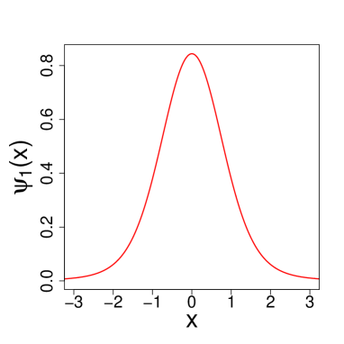
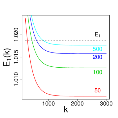
Figure 1: Cauchy oscillator ground state (left panel) and the ($k$)-time evolution of $E_{1}^{(k)}(h)=-\frac{1}{h}\ln(\mathcal{E}_{1}^{k}(h))$, (8), for $a=50,100,200,500$. The dotted line indicates the ground state eigenvalue reported in Refs. LM ; SG .

III.1 Cauchy oscillator ground state.

As the initial trial state vector we take the Hermite function $\Phi_{1}^{(0)}(x)$, (9), which is subsequently evolved up to $k=3000$, with $h=10^{-3}$. In Fig. $1$, where the Cauchy oscillator ground state is reproduced, we have intentionally abstained from depicting the corresponding $\Phi_{1}^{(k)}(x)$. The reason is that within the graphical reproduction accuracy limits, in the adopted scale and with the spatial boundary set by $a\geq 50$, the computed curve cannot be practically distinguished from the Cauchy oscillator ground state $\psi_{1}(x)$, SG . Note the visually obvious irrelevance of the boundaries: in Fig. 1 an interval $[-3,3]$ has been displayed, while $[-50,50]$ is actually considered in simulations.

For completeness we provide an analytic form of the Cauchy oscillator ground state (we recall a dimensionless form of this expression):

$$\psi_{1}(x)=\frac{A_{0}}{\pi}\int\limits_{-E_{1}}^{\infty}Ai(t)\cos x(t+E_{1})dt,$$ (10)

Here, $E_{1}=1.01879297$, while $Ai(t)$ denotes the Airy function, $A_{0}$ being a normalization factor.

The $k=3000$ approximation $E_{1}^{(k)}(0.001)$ of a ”true” eigenvalue $E_{1}$ is depicted in Fig. $1$ for values $a=50,100,200,500$ of the boundary parameter. In this case, scales have been modified to better visualize the impact of $a$ (alternatively, a contribution of longer jumps in the semigroup-driven stochastic process, as encoded in the involved Lévy measure) upon the approximation finesse of the lowest Cauchy oscillator eigenvalue $E_{1}$.

A useful hint towards the large $a$ behavior of the detuning (deviation) $\Delta E_{1}=E_{1}-E_{1}^{(k)}$ of the approximate energy value $E_{1}^{(k)}$ from the analytically derived value $E_{1}$ comes from Fig. 2, where a double logarithmic (decimal logarithm is used on both axis) scale is employed. Clearly, with the growth of $a$, the detuning value $\Delta E_{1}$ decreases.

Since the Cauchy oscillator eigenfunctions $\psi_{n}(x),n\geq 1$ obey an asymptotic estimate, KK ; LM :

$$|\psi_{n}(x)|\leqslant\frac{C_{n}}{x^{4}},\qquad|x|>1,$$ (11)

in Fig. 2 we have also displayed the graph of $x^{4}\,\Phi_{1}^{3000}(x)$ for $a=500$. The $x$-dependence in Fig. 2 has been restricted to an interval $[-100,100]$, since beyond this interval the deviation of the graph from zero quickly becomes fapp-negligible (fapp means ”for all practical purposes”).

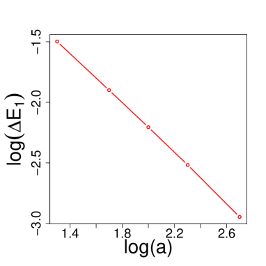
Figure 2: Detuning $\Delta E_{1}$-dependence upon $a$, in the (decimal) logarithmic scales and the behavior of $x^{4}\Phi_{1}^{(3000)}(x)$ for $a=500$.

III.2 Lowest excited states

III.2.1 $n=2$

From a formal point of view, while strictly complying with the point (i) of the algorithm (c.f. Section II.B), to recover simultaneously the ground state and the first excited state, we need to take two Hermite functions $\Phi_{1}^{(0)},\Phi_{2}^{(0)}$ as our trial states. However, there are more optimal choices as well and, given $\psi_{1}$, we can take a single Hermite function $\Phi_{2}^{(0)}$ (having one node) as a trial state and $(k)$-evolve it towards the sought for $\psi_{2}$.

In Fig. 3 the computed state function $\Phi_{2}^{(k)}(x)$ is depicted for $k=3000$. This outcome is practically (fapp) $a$-independent. As in case of the ground state, spatial boundaries in the Figure are set at $[-3,3]$, while computations have been performed for $a=50$.

An identification of $\Phi_{2}^{(k)}(x)$ as a valid approximation of a true first excited state $\psi_{2}(x)$ is supported by two arguments: (i) an analytic form of this excited state is available, and its graph cannot be visually distinguished form the depicted approximate graph, within scales adopted, (ii) the $k$-evolution of $E_{2}^{(k)}$ for different choices of $a$, displayed against the analytically supported value $E_{2}\approx 2,3381$ (dotted line), c.f. LM ; SG .

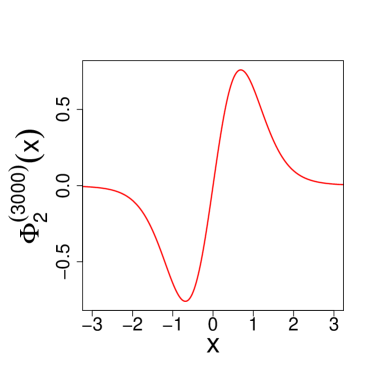
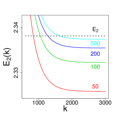
Figure 3: First excited state $\psi_{2}$ of the Cauchy oscillator and the ($k$)-time evolution of $E_{2}^{(k)}(h)$ (8) for $a=50,100,200,500$. The dotted line indicates the first excited eigenvalue reported in Refs. LM ; SG .

In Fig. 4 we have verified the validity of an asymptotic estimate (11) and the detuning $\Delta E_{2}=E_{2}-E_{2}^{(k)}$ - dependence on $a$ in a double logarithmic scale.

Let us stress that the nodal properties of the computed eigenfunction are a consequence of the oddness of the chosen trial function and do not trivially rely on the initial (trial function) number of nodes. For example, if instead of the previous odd function $\Phi_{2}^{(0)}(x)$ we would have considered its spatially translated $x\rightarrow x-1$ version

$$\frac{1}{\sqrt{2\sqrt{\pi}}}\,2(x-1)\,e^{-(x-1)^{2}/2},$$

as a trial function, then a simulation outcome would converge to the $E_{1}$ - ground state $\psi_{1}$ and not (as possibly anticipated) to the excited $E_{2}$ - state $\psi_{2}$ .

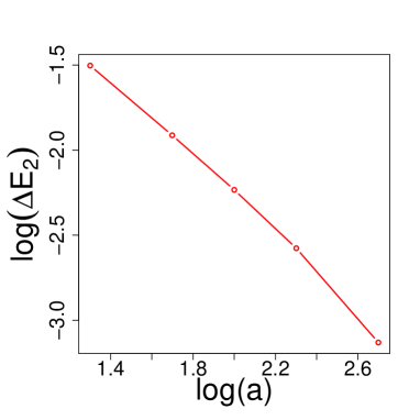
Figure 4: Detuning $\Delta E_{2}$-dependence upon $a$, in the (decimal) logarithmic scales and the behavior of $x^{4}\Phi_{2}^{(3000)}(x)$ for $a=500$.

In tune with the previous observation, let us notice that the $i=2$ Hermite function is even and has two nodes. If taken as a trial function for our algorithm, it converges to the Cauchy oscillator ground state and not to any excited state.

III.2.2 $n\geq 3$

To compute $n\geq 3$ eigenfunctions we must begin from at least two linearly independent even trial functions and follow iteratively all steps (i)-(v) of the algorithm outlined in Section II.B. If we choose as trial functions (in the notation of Eq. (9)) a two element set comprising $\Phi_{1}^{(0)}(x)$ and $\Phi_{3}^{(0)}(x)$, then the algorithm produces a sequence of state vector pairs which converges to that composed of the ground state $\psi_{1}$ and the excited state $\psi_{3}$, the latter corresponding to $E_{3}=3.24819$.

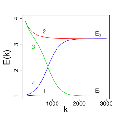
Figure 5: Two ordering choices in the Gram-Schmidt procedure. We depict the ($k$)-time evolution of $E_{i}^{(k)}$, (8), for initially chosen trial functions $\Phi_{1}^{(0)}(x)$ and $\Phi_{3}^{(0)}(x)$. For $E_{1}^{(k)}$ the (1,3) G-S order induces the black (1) curve, while blue (4) for (3,1) G-S order. For $E_{3}^{(k)}$ the (1,3) order yields the red (2) curve while (3,1) implies the green (3) one.

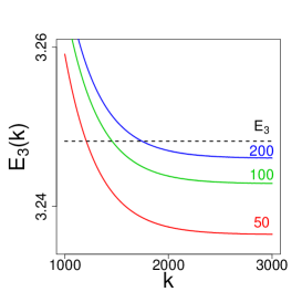
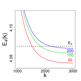
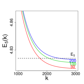
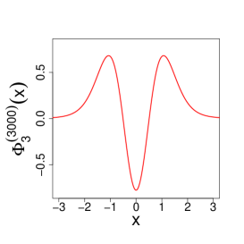
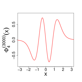
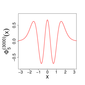
Figure 6: The $k$-evolution of $E_{i}^{(k)}$ for $i=3,4,5$ in the computation with $0\leq i\leq 4$ Hermite trial functions. The dependence on $a$ is displayed as well. The corresponding (both limiting and approximating) eigenfunctions, labeled by $i=3,4,5$, are depicted for $x\in[-3,3]$. $a\geq 50$ is used in the course of algorithmic iterations.

If the trial set is composed of $\Phi_{2}^{(0)}(x)$ and $\Phi_{4}^{(0)}(x)$ then $\psi_{2}$ together with $\psi_{4}$ will asymptotically come out. The corresponding eigenvalues read $E_{2}=2.33811$ and $E_{4}=4.08795$.

For the algorithm to work correctly, one needs to fix a priori and next secure a pre-defined order in the Gram - Schmidt orthonormalization procedure, at each $k$-th iteration. Example: in the two-element set we declare the $(1,3)$ Gram-Schmidt order. This means that in the ordered pair $\{\Phi_{1}^{(0)}(x),\Phi_{3}^{(0)}(x)\}$ after the first $h$-shift we normalize $\Psi^{(1)}_{1}(x)=S(h)\Phi_{1}^{(0)}$ and it is $\Psi_{3}^{(1)}=S(h)\Phi_{3}^{(0)}$ which is next (Gram-Schmidt)-transformed to its ultimate $\Phi_{3}^{(1)}$ form (as an orthonormal complement to $\Phi_{1}^{(1)}$). That is to be continued until a terminal $(1,3)$ ordered pair $\{\Psi^{(k+1)}_{1}=S(h)\Phi_{1}^{(k)},\Psi_{3}^{(k+1)}=S(h)\Phi_{3}^{(k)}\}$ is recovered.

In Fig. 5 we display the $k$ -evolution of $E_{i}^{(k)}$, where $i=1,3$ or $i=3,1$, in direct correspondence with the above exemplary discussion. We display as well the evolution with the reverse Gram-Schmidt order ansatz. Here $(3,1)$ means that we first normalize $\Psi_{3}^{(k)}$ and next make the G-S transformation of $\Psi_{1}^{(k)}$ to a orthonormal complement $\Psi_{1}^{(k)}$ of $\Psi_{3}^{(k)}$.

We have thus handled the ground state and three consecutive excited states up to $\psi_{4}$. The procedure in case of higher states, like e.g. $n\geq 5$, seems to need a bit more general approach. Namely, to get a $(k)$-convergent approximation of an odd eigenfunction $\psi_{5}$, we should in principle consider a trial set composed of five elements (three of them are even). This amounts to forming an initial (G-S ordered ) trial set, which is composed of five consecutive $0\leq n\leq 4$ Hermite functions.

Nonetheless, to the same end, an optimal guess is to consider merely three trial functions, say $\Phi_{1}^{(0)},\Phi_{3}^{(0)},\Phi_{5}^{(0)}$. Outcomes of algorithmic iterations are presented in Fig. 6. We display the $k$-evolution, up to $k=3000$, of $E_{i}^{(k)}$ for selected indices $i=3,4,5,$ and for values $a=50,100,200$ of the boundary parameter. We also depict the approximations (5) of the corresponding eigenfunctions $\psi_{i},i=3,4,5$ of the Cauchy oscillator, SG ; LM . We note that the plots (e.g. shapes) of approximate eigenfunctions for $a\geqslant 50$ are graphically fapp independent of $a$. Their defining properties can be read out by restricting the space axis in Fig. 6 to the interval $[-3,3]$ and (fapp ) appear to coincide with those for true eigenfunctions.

As a word of warning, let us call again our ”linear ansatz” in the Strang splitting formula (5). For higher eigenfunctions and eigenvalues, the G-S orthonormalization procedure induces an accumulation of systematic (ansatz related) errors. Therefore one should not uncritically extend our algorithm (designed with a purpose to investigate lowest parts of the spectrum) to higher parts of the spectrum.

III.3 Spatial nonlocality impact on the approximation finesse.

As mentioned repeatedly above, the usage of the algorithm involves a spatial cutoff placing the simulation outcomes in $L^{2}([-a,a])$, even if initial trial functions are elements of $L^{2}(R)$. Interestingly, the shapes of eigenfunctions appear not to be very sensitive upon the value of $a$. Indeed, all relevant numerical outcomes (see e.g. the approximate eigenfunctions plots in Figs. $1,3,6$) could have been reproduced in the space interval $[-3,3]$. Even though $a=50,100,200,500$ is employed in all integrations.

The situation appears to be different if we pass to approximate eigenvalues, where the $a$ - dependence appears to be vital. Then, convergence properties of $E_{i}^{(k)}(a)$ can be quantified by means of the detuning (deviation) value $\Delta E_{i}(a)$ which falls down with the growth of $a$, as displayed in Figs. $2$ and $4$.

We shall derive a rough estimate of the detuning dependence on $a$, based on the assumption that far beyond the boundaries of the interval $[-3,3]$, the approximate and true (limiting) eigenfunction, both corresponding to the true eigenvalue $E$, do not differ considerably.

Let $H(a)f\sim E(a)f$ sets an approximate eigenvalue solution of the original Cauchy oscillator problem. The ”kinetic” term $T(a)f$ has the form dictated by Eq. (2), provided the Cauchy principal value of the integral is evaluated in the interval $[-a,a]$, $a=50$, instead of the previously mentioned $[-3,3]$. Accordingly for $x\in[-a,a]$ we have

$$H(a)f(x)\sim[(-\Delta)^{1/2}+V(x)]\,f(x)=\frac{1}{\pi}\int_{|z|\leq a}\frac{f(x)-f(x+z)}{z^{2}}dz+V(x)f(x)\sim E(a)\,f(x).$$ (12)

Let $g(x)$ be another approximate spectral solution corresponding to the eigenvalue $E(b)$, with $b>a$, that is close to $E(a)$ (as a member of a sequence converging to the limiting/genuine eigenvalue $E$ associated with an eigenfunction $\psi(x)$).

By our $f\sim g$ assumption, a continuation of $f$ from $[-a,a]$ to $[-b,b]$ does not differ considerably from $g$ well beyond the control interval $[-3,3]$ (c.f. Figs. 1, 3, 6). We additionally assume the same about $V(x)g(x)$ (for $V(x)\sim x^{2}$ this would need $g(x)\ll 1/x^{2}$, in consistency with the estimate (11)). Therefore for $x\in[-b,b]$ we have (keeping in mind that we evaluate the Cauchy principal value of the integral):

$$H(b)g(x)\sim{\frac{1}{\pi}}\int_{|z|\leq b}{\frac{g(x)-g(x+z)}{z^{2}}}dz+V(x)g(x)\sim E(a)\,g(x)+\frac{1}{\pi}\int_{a\leq|z|\leq b}\frac{g(x)-g(x+z)}{z^{2}}dz\sim$$ (13)

$$E(a)\,g(x)+{\frac{2}{\pi}}\,g(x)\,\int_{a}^{b}{\frac{dz}{z^{2}}}\sim\left[E(a)+{\frac{2}{\pi}}\left({\frac{1}{a}}-{\frac{1}{b}}\right)\right]\,g(x)\sim E(b)g(x)$$

Hence

$$E(b)-E(a)\sim{\frac{2}{\pi}}\left({\frac{1}{a}}-{\frac{1}{b}}\right).$$ (14)

Inserting consecutive boundary values $50,100,200,500$ in the above formula we arrive at a perfect agreement with the numerically retrieved $E(b)-E(a)$ data. Namely, we have: $(2/\pi)(1/50-1/100)\sim 0.0064$, $(2/\pi)(1/100-1/200)\sim 0.0032$, $(2/\pi)(1/200-1/500)\sim 0.0019$ and ultimately $(2/\pi)(1/500-1/\infty)\sim 0.0013$.

We can readily reproduce the detuning $\Delta E(a)=E-E(a)$ dependence on $a$, as depicted in Figs. $1$ through $6$, provided the $k$-instant of the numerically implemented evolution is common for all $E(a)$.

IV Cauchy well eigenvalue problem

A primary motivation for the present research have been inconsistencies and erroneous statements detected in publications devoted to selected fractional QM spectral problems, the harmonic potential and the infinite well problem being included. Spectral solutions for the infinite well presented in Refs. DX ; B ; D are incorrect. See e.g. YL ; J ; Z ; GS for a discussion of some of those issues, specifically in connection with a correct spatial shape of the pertinent eigenfunctions.

We take a constructive attitude and instead of reproducing a list of faulty statements, we shall directly address the finite and next infinite well problem in the fractional QM, for an exemplary Cauchy case. The main methodology will based on the previously tested algorithm, but our approach will directly refer to the finite well in the nonlocal (fractional) context. Subsequently (like in GK where a similar route has been followed in the local QM) we shall pass from a shallow to a very deep (eventually infinitely deep) well.

Since approximate spectral formulas and eigenfunction estimates are available for the the ”fractional Laplace operator in the interval” (mathematicians’ transcript of the infinite well in fractional QM), K , the latter publication will be our reference point as far as an approximation issue of an infinite well in terms of a sequence of deepening finite wells, will become our concern.

If we choose in Eqs. (1) and (2) the potential $V(x)$ in the form

$$V(x)=\left\{\begin{array}[]{ll}0,&\hbox{$|x|<1$;}\\ V_{0},&\hbox{$|x|\geqslant 1$.}\end{array}\right.$$ (15)

where $V_{0}>0$, we tell about the Cauchy well spectral problem.

In case of the Cauchy well, our numerical algorithm (i)-(v) allows to deduce approximate eigenvalues and eigenfunctions of the pertinent spectral problem. Since an infinite well limit, to which we continually refer, can be formulated in terms of $L^{2}([-a,a])$ (see however GK for another viewpoint in the local context), we quite intentionally choose an initially pre-defined trial set of linearly independent functions to be an orthonormal basis in $L^{2}[-1,1]$ whose trivial extension to $L^{2}(R)$ reads as follows:

$$\Phi_{n=2m+1}^{(0)}(x)=\left\{\begin{array}[]{ll}A\cos\left(\frac{n\pi x}{2}\right),&\hbox{$|x|<1$,}\\ 0,&\hbox{$|x|\geqslant 1$}\end{array}\right.\qquad\Phi_{n=2m}^{(0)}(x)=\left\{\begin{array}[]{ll}A\sin\left(\frac{n\pi x}{2}\right),&\hbox{$|x|<1$,}\\ 0,&\hbox{$|x|\geqslant 1$}\end{array}\right.\qquad m=0,1,\ldots$$ (16)

The normalization constant $A$ equals $\pm 1$. A particular sign choice has no physical meaning, but to compare our simulation outcomes with results of other publications, sometimes a concrete sign adjustment is necessary (to be explicitly stated when necessary).

Remark 5: The above orthonormal basis in $L^{2}([-1,1])$ has been claimed in Refs. DX ; B ; D to comprise eigenfunctions of the infinite Cauchy well problem with boundaries at the ends of $[-1,1]$ and the eigenvalues $E_{n}=n\pi/2$. These statements we shall openly disprove in below, see e.f. Fig. 7, and as a constructive part of the argument we shall provide numerically deduced, actual eigenvalues and shapes of the respective eigenfunctions. The level of accuracy for low lying eigenstates is surprisingly good. It is worthwhile to mention that the only eigenvalue formulas for an infinite Cauchy well, that can be termed rigorous, refer to the large $n$ limit. More explicitly K we actually have an approximate expression for $E_{n}$, provided $n$ is sufficiently large:

$$E_{n}={\frac{n\pi}{2}}-{\frac{\pi}{8}}+O\left({\frac{1}{n}}\right).$$

For completeness of arguments, let us give an explicit expression for approximate eigenfuctions associated with the large $n$ part of the infinite Cauchy well spectrum. Namely, we have (with minor adjustments of the original notation of Ref. K ):

$$\psi_{n}(x)=q(-x)F_{n}(1+x)-(-1)^{n}q(x)F_{n}(1-x),\qquad x\in R,$$

where $E_{n}=\frac{n\pi}{2}-\frac{\pi}{8}$ and $q(x)$ is an auxiliary function

$$q(x)=\left\{\begin{array}[]{ll}0&\hbox{for $x\in(-\infty,-\frac{1}{3})$,}\\ \frac{9}{2}\left(x+\frac{1}{3}\right)^{2}&\hbox{for $x\in(-\frac{1}{3},0)$,}\\ 1-\frac{9}{2}\left(x-\frac{1}{3}\right)^{2}&\hbox{for $x\in(0,\frac{1}{3})$,}\\ 1&\hbox{for $x\in(\frac{1}{3},\infty)$.}\end{array}\right.$$

The function $F_{n}(x)$ is defined as follows: $F_{n}(x)=\sin\left(E_{n}\,x+\frac{\pi}{8}\right)-G(E_{n}\,x)$, where $G(x)$ is the Laplace transform $G(x)=\int\limits_{0}^{\infty}e^{-xs}\gamma(s)ds$ of a positive definite function $\gamma(s)$:

$$\gamma(s)=\frac{1}{\pi\sqrt{2}}\frac{s}{1+s^{2}}\exp\left(-\frac{1}{\pi}\int\limits_{0}^{\infty}\frac{1}{1+r^{2}}\log(1+rs)dr\right).$$

Evidently, things are here much more complicated than an oversimplified (and faulty) guess (16) of previous authors would suggest.

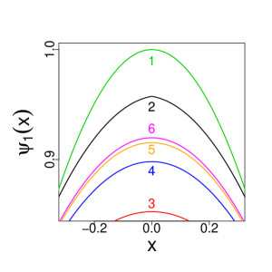
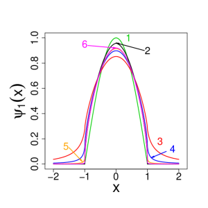
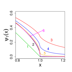
Figure 7: Ground state solution of the Cauchy well. Numbers refer to: 1 - $\cos(\pi x/2)$, 2 - an approximate solution, Eq. (13) in K , 3,4,5,6 refer to the well depths, respectively $5,20,100,500$. Convergence symptoms (towards an infinite well solution) are visually identifiable. Left panel reproduces an enlarged resolution around the maximum of the ground state. The right panel does the same job in the vicinity of the right boundary $+1$ of the well (curves deformation comes from scales used to increase a resolution).

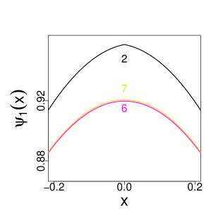
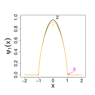
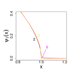
Figure 8: Convergence towards $\psi_{1}$: 2 - an approximate ground state, Eq. (13) in K ; Our algorithm appears to be more reliable, since $6$ and $7$ refer to wells whose depths are respectively $500$ and $5000$. Left panel shows an enlarged vicinity of the maxima. Right panel shows enlarged plots in the vicinity of $+1$.

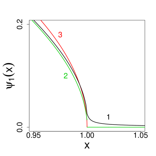
Figure 9: Finite versus infinite Cauchy well ground state in the vicinity of the boundary $+1$ of $[-1,1]$: 1 (black) - the algorithm outcome for the finite $V_{0}=500$ well, 2 (green) - an approximate infinite well expression from Ref. K , 3 (red) - an approximate form of $\psi_{1}(x)\sim(1-|x|)^{1/2}$, in the vicinity of the infinite well barriers, as proposed in Ref. Z .

IV.1 Ground state

As the initial trial function in $L^{2}(R)$ we take $\Phi_{1}^{(0)}(x)=cos(\pi x/2)$ for $|x|<1$ and $0$ otherwise, see Eq. (16). Without further mentions of the detailed (i)-(v) algorithm steps (c.f. Sections II.B and C), we shall immediately pass to a discussion of results obtained by means of numerical procedures. We note that the action of $S(h)$, Eq. (6), defined in $L^{2}(R)$, effectively now takes us away from $L^{2}([-1,1])$ trial functions to elements of $L^{2}([-a,a])$, where $a>1$ sets actual integration boundaries. Typically we have $a\geq 50$.

In Fig. 7 approximations of the finite well ground state $\psi_{1}$ are depicted for few well depths. Namely: $V_{0}=5$ (red, $3$), $V_{0}=20$ (blue, $4$), $V_{0}=100$ (orange, $5$), $V_{0}=500$ (pink, $6$). These outcomes need to be compared with an apparently faulty solution proposed in Refs DX ; B ; D (green, $1$) and an approximate ground state in the infinite well as provided in Ref. K (black, $2$).  Left panel amplifies the differences in the vicinity of a maximum of $\psi_{1}$, while the right panel amplifies them in the vicinity of the right boundary of the well (e.g. about $+1$). Chosen scales slightly deform the actual shapes of curves, but that is the price paid for an amplification of differences between closely packed curves.

We have clearly confirmed (see curves $3$, $4$, $5$ and $6$) a convergence towards an infinite well ground state $\psi_{1}$. Effectively it is the curve $6$ corresponding to $V_{0}=500$ that suffices to identify a proper shape and a spatial location of the curve representing the infinite well ground state $\psi_{1}$.

To get a better insight into the convergence issue, in Fig. $8$ we directly compare approximate ground states that were derived numerically for $V_{0}=500$ (pink, $6$) and $V_{0}=5000$ (yellow, $7$). For comparison, an approximate curve drawn on the basis of K is displayed. Left panel refers to a vicinity of a maximum of $\psi_{1}$, while the right one to the vicinity of the well boundary.

For finite wells, quite in affinity with the standard local spectral problem, eigenfunctions ”spread out” well beyond the well area $[-1,1]$, especially for shallow wells. Fig. 7 decisively demonstrates that $\cos(\pi x/2)$ is not a spectral solution (e.g. ground state) for an infinite well problem (see e.g. curve 1). It is the vicinity of the curves 5 and 6, where the true infinite well ground state is actually located. Compare e.g. Fig. 8 where the depth of the well has been lifted from $500$ to $5000$. An approximate solution K (curve 2 in Fg. 7) differs considerably from a true ground state in the central area of the well while at the well boundaries, together with all other curves appears to converge to a true ground state for $V_{0}>100$ (comparison curves are numbered 5 and 6).

Remark 6: For $V_{0}=5000$ our computer algorithm appears to accumulate errors coming from the low-order Strang splitting choice and small-valued cutoffs finesse. That appears not to be significant for the shape of eigenfunctions. In Fig. 8 we note quite indicative agreement at the boundaries with the approximating curve of K . Somewhat unfortunately, the accuracy becomes significantly worse when it comes to the computation of eigenvalues, especially for $n>3$. That issue will be discussed later.

The well spatial extension is limited to $[-1,1]$. It seems instructive to know what the concrete values (at prescribed points) of eigenfunctions are beyond this interval. This indicates how fast is the decay of the ground state beyond $[-1,1]$. In Table I we have collected ground state values at points $x=2,10,40,50$ for various choices of $V_{0}$.

	2	10	40	50
5	$3.7\cdot 10^{-2}$	$1.3\cdot 10^{-3}$	$8.3\cdot 10^{-5}$	$5.4\cdot 10^{-5}$
20	$7.3\cdot 10^{-3}$	$2.4\cdot 10^{-4}$	$1.5\cdot 10^{-5}$	$9.6\cdot 10^{-6}$
100	$1.3\cdot 10^{-3}$	$4.4\cdot 10^{-5}$	$2.7\cdot 10^{-6}$	$1.7\cdot 10^{-6}$
500	$2.6\cdot 10^{-4}$	$8.6\cdot 10^{-6}$	$5.3\cdot 10^{-7}$	$3.4\cdot 10^{-7}$

Table 1: Values of $\psi_{1}(x)$ for $x=2,10,40,50$ and $V_{0}=5,20,100,500$.

We note a fast convergence of $\psi_{1}(x)$ to $0$, outside of $[-1,1]$. This confirms an antcipated $V_{0}\to\infty$ outcome that $\psi_{1}(x)$ equals identically zero beyond $(-1,1)$. The pertinent limit should be understood in the Cauchy sense: for each $\varepsilon>0$ there exists $\delta>0$ such that for all $x\in(-\infty,-1]\cup[1,\infty)$, if only $V_{0}>\delta$, there holds $|\Phi_{1}^{(k)}(x)|<\varepsilon$.

In Table II, asymptotic (approximate) finite well eigenvalues are displayed for $V_{0}=5,20,100,500,5000$ and integration intervals set by $a=50,100,200,500$.

	5	20	100	500	5000
50	0.9538	1.0743	1.1258	1.1408	1.1445
100	0.9602	1.0807	1.1322	1.1472	1.1509
200	0.9634	1.0839	1.1353	1.1504	1.1541
500	0.9653	1.0858	1.1372	1.1523	1.1560

Table 2: Approximate ground state eigenvalue for various well depths $V_{0}$ and integration volume bounds $a$. The data for $V_{0}=5000$ were computed with the time step h=0.001.

We note that the variability of eigenvalues as functions of $a$ does not depend on the well depth. Clearly $E(100)-E(50)\sim 0.0064$, $E(200)-E(100)\sim 0.0032$, $E(500)-E(200)\sim 0.0019$. These data stay in a precise coincidence with the previously discussed effect of extending integration boundary well beyond the (small) control interval in the Cauchy oscillator case, see e.g. (13) and (14).

As directly seen in Table II, the approximate ground state eigenvalues grow up with the well depth. Tht is not unexpected. The largest value we are sure is sufficiently accurate reads $1.1523$ and corresponds to $V_{0}=500$.
The value corresponding to $V_{0}=5000$ is less accurate, in view of errors accumulated in the numerical procedure. The well depth is so large that we can directly compare this value with that for an infinite well produced in Ref. K , see Table 2 there in. To improve the fidelity level for $V_{0}=5000$, we need the time partition unit to be one order less (i.e. h= 0.0001) than actually chosen h=0.001. This decision would significantly increase the simulation time.

IV.2 Low-lying excited states

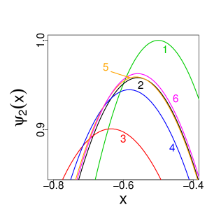
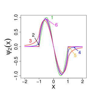
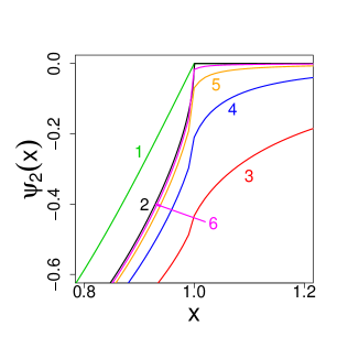
Figure 10: First excited state $\psi_{2}$. Numbers refer to: 1 - $-\sin(\pi x)$, 2 - an approximate solution (13) of Ref. K , 3, 4, 5, 6 correspond to finite wells with depths $V_{0}=5,20,100,500$ respectively. In the left panel we display an enlarged vicinity of the maximum of $\psi_{2}$. The right panel contains an enlargement of closely packed curves in the vicinity of the right boundary $1$ of the well. Note the scales employed.

	5	20	100	500	5000
50	2.3701	2.6060	2.7046	2.7343	2.7419
100	2.3765	2.6124	2.7110	2.7407	2.7483
200	2.3797	2.6156	2.7142	2.7439	2.7515
500	2.3816	2.6175	2.7161	2.7458	2.7534

Table 3: The approximate eigenvalue $E_{2}$ for various well depths $V_{0}$ and $a$.

To deduce the first excited level of the finite well (if in existence, we have checked that the shallow well with $V_{0}=5$ has three bound states), we take $\Phi_{1}^{(0)}(x)=-\sin(\pi x)$ for $|x|<1$ and $0$ otherwise, see Eq. (16) as a trial function. For comparison with Ref. K we have chosen the minus sign instead of the positive one. In Fig. 10 the first excited state $\psi_{1}$ has been depicted (colors, curves numbering being the same as in the ground state displays in Fig. 7).

We have a clear confirmation that would be infinite well eigenfunctions of Refs. DX ; B ; D are plainly wrong (curve 1). Our approximate eigenfunctions show a definite convergence towards an asymptotic (true infinite well) eigenfunction, see e.g. curves 5 and 6. An approximate eigenfunction of Ref. K is much better approximation of a true excited eigenstate, than it was in case of the ground state. Nonetheless there are obvious deviations from the true shape of the eigenstate in the vicinity of the well boundaries (lets panel, curves 2 and 6 need to be compared).

We anticipate that with the increase of $V_{0}$ the obtained modifications of the shape of the curve 6, in the vicinity of its extrema, would be insignificant. The behavior in the vicinity of the well boundaries would be more indicative. Compare e.g. Fig. 9 depicting the ground state of the ”almost” infnite well.

In Table III we have collected approximate eigenvalues of $\psi_{2}$ for various well depths $V_{0}$ and integration boundary values $a$. Again, we observe that the variability of eigenvalues as functions of $a$ does not depend on the well depth. The data stay in a precise coincidence with the previously discussed effect of extending integration boundary well beyond the (small) control interval in the Cauchy oscillator case, see e.g. (13) and (14). The approximate eigenvalue of $\psi_{2}$ grow together with $V_{0}$.

The largest numerical outcomes that correspond to $V_{0}=500$ and $V_{0}=5000$ can be directly compared with values reported in Table 2 of Ref. K . As a complement to this discussion, subsequently (Table VII) we shall compare our maximal approximate eigenvalues with best (optimal) approximations reported in Ref. K .

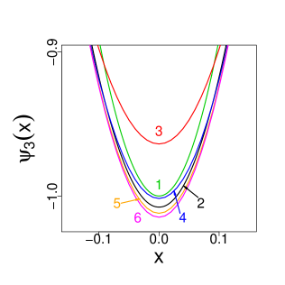
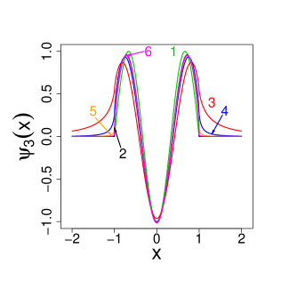
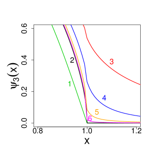
Figure 11: Eigenstate $\psi_{3}$. Numbers refer to: 1 - $-\cos(3\pi x/2)$, 2 - approximate solution (13) of Ref. K , 3, 4, 5, 6 correspond to well depths $V_{0}=5,20,100,500$. Left panel contains an enlargement of a minimum of $\psi_{3}$. Right panel depicts an enlargement of closely packed curves in the vicinity of the well boundary.

0

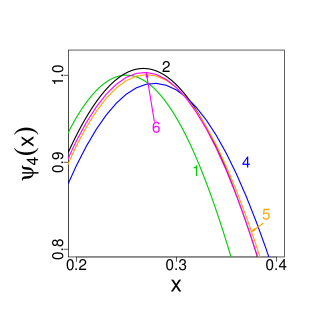
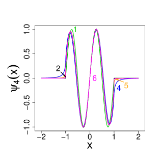
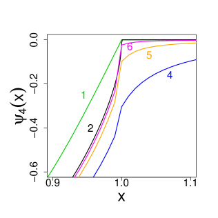
Figure 12: Eigenstate $\psi_{4}$. Numbers correspond to: 1 - $\sin(2\pi x)$, 2 - approximate solution (13) of Ref. K , 4, 5, 6 refer to $V_{0}=20,100,500$. Left panel depicts the vicinity of a maximum of $\psi_{4}$. Right panel refers to the well boundary.

	5	20	100	500	5000
50	3.7457	4.1116	4.2517	4.2942	4.3053
100	3.7522	4.1180	4.2581	4.3006	4.3117
200	3.7554	4.1212	4.2613	4.3038	4.3149
500	3.7573	4.1231	4.2632	4.3057	4.3168

	5	20	100	500	5000
50	-	5.6378	5.8147	5.8687	5.8830
100	-	5.6442	5.8211	5.8751	5.8894
200	-	5.6474	5.8243	5.8783	5.8926
500	-	5.6493	5.8262	5.8802	5.8945

Table 4: Approximate values for $E_{3}$ and $E_{4}$ for various $V_{0}$ and $a$. The $V_{0}=5$ well has three bound states only.

	5	20	100	500	5000
50	-	7.1584	7.3720	7.4369	7.4543
100	-	7.1648	7.3784	7.4433	7.4607
200	-	7.1680	7.3816	7.4465	7.4639
500	-	7.1699	7.3835	7.4484	7.4658

	5	20	100	500	5000
50	-	8.6878	8.9359	9.0109	9.0312
100	-	8.6942	8.9423	9.0173	9.0376
200	-	8.6974	8.9455	9.0205	9.0408
500	-	8.6993	8.9474	9.0224	9.0427

Table 5: Approximate values for $E_{5}$ and $E_{6}$.

	5	20	100	500	5000
50	-	10.2136	10.4979	10.5827	10.6057
100	-	10.2200	10.5043	10.5891	10.6121
200	-	10.2232	10.5075	10.5923	10.6153
500	-	10.2251	10.5094	10.5942	10.6172

	5	20	100	500	5000
50	-	11.7443	12.0638	12.1579	12.1836
100	-	11.7507	12.0702	12.1643	12.1900
200	-	11.7539	12.0734	12.1675	12.1932
500	-	11.7558	12.0753	12.1694	12.1951

Table 6: Approximate eigenvalues for $E_{7}$ and $E_{8}$.

	$E_{1}$	$E_{2}$	$E_{3}$	$E_{4}$	$E_{5}$	$E_{6}$	$E_{7}$	$E_{8}$
Ref.K	1.1577	2.7547	4.3168	5.8921	7.4601	9.0328	10.6022	12.1741
$a=500,\,V_{0}=500$	1.1523	2.7458	4.3057	5.8802	7.4484	9.0224	10.5942	12.1694
$a=500,\,V_{0}=5000$	1.1560	2.7534	4.3168	5.8945	7.4658	9.0427	10.6172	12.1951

Table 7: A comparison of our approximate eigenvalues for a $V_{0}=500,\,a=500$ with ”most optimal” values presented in Ref. K .

To deduce other excited states and corresponding eigenvalues an algorithm needs to be used in its full extent, with a properly chosen initial set of trial functions and theri consecutive Gram-Schmidt orthonormalization at each iteration step. In Figs 11 and 12 we depict shapes of the third and fourth finite well eigenstates (in the well $V_{0}=5$ three bound states are in existence). Tables IV-VI collect the data for six consecutive eigenvalues (up to $n=8$). Again, we have clearly confirmed that would-be infinite well eigenfunctions of Refs DX ; B ; D are plainly wrong. Albeit, per force, one can admit some level of robustness, at which those can be viewed as very robust approximations of a true state of affairs.

In Table VII we have compared maximal simulated eigenvalues, obtained for $V_{0}=500$, $V_{0}=5000$ and $a=500$, with optimal approximations reported in Ref. K . Our numerical values of Table VII, in case of $V_{0}=500$ are slightly lower than those in Table 2 of Ref. K , as expected. Namely, our computed values refer to finite wells, while the data of Ref. K refer to an infinite well. We can make a rough guess that the computed value for $a=500$, might differ by about $0.0013$ from an infinite well eigenvalue (c.f. our previous $E(a)-E(b)$ discussion).

Remembering about a remark we have made before about an accumulation of numerical errors when we pass to higher eigenstates and eigenvalues (they are basically a consequence of the Gram-Schmidt orthonormalization procedure), we may look at respective eigenvalues from this ”error accumulation” perspective. A comparison of our numerical results in the $V_{0}=5000$ case with approximate eigenvalues of Ref. K indicates that, beginning from $n=4$, our procedure shows up some limitations and needs improvements (those are known for practitioners of analogous algorithms in the local case). The resultant eigenvalues become too large, compared with our anticipation. The simplest way to improve our numerics would be to chose so small time step $h$, such that for larger $V_{0}$ we would have at least $hV_{0}<1$, and even better if $hV_{0}<1/2$.

V Outlook

Our numerically-assisted derivation of eigenfunctions and eigenvalues may be adopted to any nonlocal problem (e.g. any fractional or quasi-relativistic motion generator), not only in 1D but also in 2D or 3D. There is no basic limitation upon the choice of the external confining potential $V(x)$. The main model-dependent factors are the time interval partition unit $h$ and the size of integration volume (that was $a$ in our 1D case, while an arbitrary finite open volume in $R^{3}$ is admitted). They affect the ultimate numerical outcomes.

Coming back to our 1D considerations, an important issue is that of seeking an optimum: small time partition unit $h$ versus large $V_{0}$. In particular, for fairly small $h$, higher Taylor series terms can be accounted for in the Strang splitting method. It is know that in the local case, the fourth-order algorithm works pretty well Auer .

For the finite well potential (15) the time step $h$ needs to be adjusted to $V_{0}$ so that $h\,V_{0}$ is ”small enough”. In the present paper we were mostly interested in the precise deduction of lowest eigenstates and eigenvalues. To this end, the choice of $h=0.001$ and well depths $V_{0}=5\,,20\,,100\,,500$ proved to be optimal.

As we have mentioned before our decision to employ the Gram-Schmidt orthonormalization procedure at each step of the algorithm proved to be a source of accumulating errors. Other procedures are known to be more reliable. However, we have been seeking for an optimal choice between various error-producing factors and the simulation time. For lowest eigenstates the G-S choice was optimal in this respect.

The major goal of the paper, that of disproving faulty results concerning the infinite well spectrum has been achieved. We have produced a number of high accuracy numerically-assisted approximations of ”true” finite and (ultimately) infinite Cauchy well eigenstates. A comparison with approximate results obtained in the mathematical literature K , proved an efficiency of both our computation method and the reliability of its outcomes.

References

- (1) P. Garbaczewski and V. A. Stephanovich, Lévy flights and nonlocal quantum dynamics, J. Math. Phys. 54, 072103, (2013).
- (2) K. Kowalski and J. Rembielinski, Salpeter equation and probability current in the relativistic quantum mechanics, Phys. Rev. A 84, 012108, (2011).
- (3) Zhi-Feng Li et al, Relativistic harmonic oscillator, J. Math. Phys. 46, 103514, (2005).
- (4) N. Laskin, Fractional quantum mechanics, Phys. Rev. 62, 3135, (2000).
- (5) N. Laskin, Fractional Schrödinger equation, Phys. Rev. E 66, 056108, (2002).
- (6) J. Dong and M. Xu, Applications of continuity and discontinuity of a fractional derivative of the wave functions to fractional quantum mechanics, J. Math. Phys. 49, 052105, (2008).
- (7) S. S. Bayin, On the consistency of the solutions of the space fractional Schrödinger equation, J. Math. Phys. 53, 042105, (2012), ibid 53, 084101, (2012).
- (8) J. Dong, Lévy path integral approach to the solution of the fractional Schrödinger equation with infinite square well, arXiv:1301.3009v1.
- (9) Y. Luchko, Fractional Schrödinger equation for a particle moving in a potential well, J. Math. Phys. 54, 012111,(2013).
- (10) M. Jeng et al, On the nonlocality of he fractional Schrödinger equation, J. Math. Phys. 51, 062102, (2010).
- (11) A. Zoia, A. Rosso and M. Kardar, Fractional Laplacian in a bounded domain, Phys. Rev. E 76, 021116,(2007).
- (12) R. Bañuelos and T. Kulczycki, The Cauchy process and the Steklov problem, J. Funct. Anal. 211, 355, (2004).
- (13) K. Kaleta and T. Kulczycki, Intrinsic ultracontractivity for Schrödinger operators based on fractional Laplacian, Potential Anal. 33, 313, (2010).
- (14) A. N. Hatzinikitas, Spectral properties of the Dirichlet operator on domains in d-dimensional Euclidean space, J. Math. Phys. 54, 103501, (2013).
- (15) T. Kulczycki, M. Kwa nicki, J. Ma ecki and A. Stós, Spectral properties of the Cauchy process on half-line and interval, Proc. London Math. Soc. 101, 589, (2010).
- (16) M. Kwaśnicki, Eigenvalues of the fractional Laplace operator in the interval, J. Funct. Anal. 262, 2379, (2012).
- (17) P. Garbaczewski and W. Karwowski, Impenetrable Barriers and Canonical Quantization, Am. J. Phys. 72, 924,(2004).
- (18) P. Bader, S. Blanes and F. Casas, Solving the Schrödinger eigenvalue problem by the imaginary time propagation technique using splitting methods with complex coefficients, J. Chemical Physics 139, 124117 (2013).
- (19) M. Aichinger and E. Krotscheck, A fast configuration space method for solving local Kohn –Sham equations, Computational Materials Science, 34, 188, (2005).
- (20) J. Auer and E. Krotschek, A fourth-order real-space algorithm for solving local Schrödinger equations, J. Chem. Phys. 115, 6841, (2001).
- (21) S. Janaecek and E. Krotscheck, A fast and simple program for solving local Schrödinger euqations in two and three dimensions, Comp. Phys. Comm. 178, 835, (2008).
- (22) S. A. Chin, S. Janecek and E. Krotscheck, An arbitrary order diffusion algorithm for solving Schrödinger equation, Comp. Phys. Comm. 180, 1700, (2009).
- (23) P. Amore et al. Collocation method for fractional quantum mechanics, J. Math. Phys. 51, 122101, (2010).
- (24) P. Garbaczewski and V. A. Stephanovich, Levy flights in inhomogeneous environments, Physica A 389, 4419, (2010).
- (25) J. Lőrinczi and J. Ma ecki, Spectral properies of the massless relativistic harmonic oscillator, J. Differential Equations, 253, 284, (2012).
- (26) K. Kowalski and J. Rembielnski, Relativistics massless harmonic oscillator, Phys. Rev. A 81, 012118, (2010).
- (27) P. Garbaczewski and V. A. Stephanovich, Lévy targeting and the principle of detailed balance, Phys. Rev. E 84, 011142, (2011).
- (28) R. N. Mantegna and H. E. Stanley, Stochastic Process with Ultraslow Convergence to a Gaussian: The Truncated L vy Flight, Phys. Rev. Lett. 73, 2946, (1994).