Transaction Repair: Full Serializability Without Locks

Abstract

Transaction Repair is a method for lock-free, scalable transaction processing that achieves full serializability. It demonstrates parallel speedup even in inimical scenarios where all pairs of transactions have significant read-write conflicts. In the transaction repair approach, each transaction runs in complete isolation in a branch of the database; when conflicts occur, we detect and repair them. These repairs are performed efficiently in parallel, and the net effect is that of serial processing. Within transactions, we use no locks. This frees users from the complications and performance hazards of locks, and from the anomalies of sub-serializable isolation levels. Our approach builds on an incrementalized variant of leapfrog triejoin, an algorithm for existential queries that is worst-case optimal for full conjunctive queries, and on well-established techniques from programming languages: declarative languages, purely functional data structures, incremental computation, and fixpoint equations.

1 introduction

1.1 Scenario

Consider the following artificial scenario chosen to highlight essential issues. A database tracks available quantities of warehouse items identified by sku number (stock-keeping unit). Each transaction adjusts quantities for a subset of skus, updating a database predicate $\mathsf{inventory}[\mathsf{sku}]=\mathsf{qty}$. Suppose there are $n$ skus, and each transaction adjusts skus chosen independently with probability $\alpha n^{-1/2}$. Most pairs of transactions will conflict when $\alpha\gg 1$: the expected number of skus common to two transactions is $E[\cdot]=n\cdot\left(\alpha n^{-1/2}\right)^{2}=\alpha^{2}$, an instance of the Birthday Paradox.

Row-level locking is a bottleneck when $\alpha\gg 1$: since most transactions have skus in common, they quickly encounter lock conflicts and are put to sleep. Figure 1 (left) shows parallel speedup of transaction throughput for $\alpha=0.1$, $\alpha=1.0$, and $\alpha=10$, using an efficient implementation of row-level locking on a multicore machine. Note that for $\alpha=10$ there is no parallel speedup: there are so many conflicts that throughput is reduced to that of a single cpu.

Our approach, which we call transaction repair, is rather different. The LogicBlox database has been engineered from the ground-up to use purely functional and versioned data structures. Transactions run simultaneously, with no locking, each in complete isolation in its own branch of the database. We then detect conflicts and repair them. These repairs are performed efficiently in parallel, and the net result is a database state indistinguishable from sequential processing of transactions. With this approach, we are able to achieve parallel speedup even when there are large amounts of conflicts between transactions (Figure 1, right).

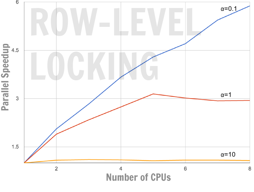
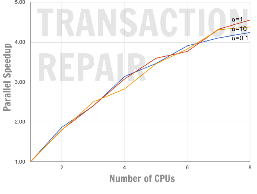
Figure 1: (a) Parallel speedup for the scenario of Section 1.1, using an efficient implementation of row-level locking. When the expected number of conflicts between two transactions is small ($\alpha=0.1$), parallel speedup for a modest number of processors is possible, since most transactions can get some work done before encountering a lock conflict. For $\alpha=1$, parallel speedup is sharply limited; and for $\alpha=10$ almost no speedup is possible, since every transaction immediately encounters a lock conflict. (b) Parallel speedup for the same scenario, using transaction repair. (Speedup of our current prototype is hindered by contention in memory allocation subroutines; this is unrelated to repair per se.)

It does not strain credulity to report that transaction repair can achieve parallel speedup for the trivial scenario just described. Remarkably, our technique applies to arbitrary mixtures of complex transactions.

1.2 Transaction repair

Transaction repair combines three major ingredients:

1. Leapfrog triejoin: Each transaction in our system consists of one or more rules written in our declarative language LogiQL, a substantial augmentation of Datalog which preserves the clean lines of the original. Each LogiQL rule is evaluated using leapfrog triejoin, an algorithm for existential rules for which a significant optimality property was recently proven [14].

2. Incremental maintenance of rules: Leapfrog triejoin admits an efficient incremental maintenance algorithm that is designed to achieve cost proportional to the trace-edit distance of leapfrog triejoin traces [13]. We employ this algorithm to repair individual rules when conflicts occur between transactions. In operation, the maintenance algorithm collects sensitivity indices that precisely specify database state to which a rule is sensitive, in the sense that modifying that state could alter the observable outcomes of the transaction. Maintenance of individual rules is extended to maintenance of entire transactions by propagating changes through a dependency graph of the transaction rules (Section 5).

The third ingredient is transaction repair circuits, which we broadly outline in Section 1.4, and describe in detail in subsequent sections.

A bottom-up exposition would begin at the level of single rules and leapfrog triejoin, and describe how transaction repair is built on these foundations. However, the novelty of this paper is in the higher-level aspects of transaction repair; we begin there since the principles can be understood while abstracting away the detailed mechanics of individual transactions. We return to leapfrog triejoin and its incremental maintenance in Section 4. In Section 5 we cover the middle ground between rules and transaction repair, namely, the repair mechanisms that are employed inside the boundaries of a single transaction.

1.3 Advantages

Transaction repair promises significant advantages over existing approaches to concurrency control:

Simplicity. We present the simplest possible concurrency model to users: from their vantage point, transactions behave as if processed one at a time, but they enjoy the performance benefits of parallelism. There are no locks, and hence no lock interactions, no transactions aborted due to lock conflicts, and no locking strategies to select or tune. Since transaction repair provides full serializability, users are freed from the anomalies, hazards, performance tradeoffs and anxieties of sub-serializable isolation levels. Unlike Multi-Version Concurrency Control (MVCC) [2], we only abort transactions if integrity constraints fail.

Performance. We are able to achieve parallel speedup even in inimical scenarios, for example, all pairs of transactions having significant conflicts. This improves on Optimistic Concurrency Control (OCC) [11]. OCC employs readsets, somewhat analogous to our sensitivity signals. However, when conflicts are detected, OCC restarts transactions, rather than repairing them as we do. This causes OCC to perform poorly when there is significant conflict between transactions.

Economics. Our approach to transaction processing is inherently scalable. Since we do not use locks for concurrency control, we do not require low-latency communication between compute nodes to confer over locks and versioning. This suggests that transaction repair may be able to achieve transaction throughput on inexpensive clusters that rivals that of traditional databases on high end hardware.

1.4 Transaction Repair Circuits

We introduce the basic concepts of transaction repair at a casual level of detail, with pointers to later sections where the concepts are developed in depth.

We can view a transaction as a black box which inputs an initial database state and outputs changes to the database we call deltas (Figure 2(a)). Suppose we run two transactions independently in parallel. We have to be concerned that the second transaction in the proposed serialized order tries to read some state affected by deltas of the first transaction. To address this, transactions report their sensitivities, that is, aspects of database state whose modification might alter the outcome of the transaction. We compare the deltas produced by the first transaction to sensitivities declared by the second, to test whether there is a possibility of conflict. If so we describe relevant corrections of the database state (Figure 2(b)) to the second transaction, which is then repaired (incrementally maintained) for the corrections (Sections 4, 5).

Figure 2(b) is a simple example of a transaction repair circuit. It is not a circuit in the sense of custom hardware, but rather a schematic describing the work to be performed; in particular, it specifies a set of recursive fixpoint equations to be solved (Section 3). The deltas, corrections, and sensitivities are signals (Section 2.3). The triangle element is a correction operator: it takes as inputs changes to the database state (in this case, deltas) and declared sensitivities, and selects just those deltas that match sensitivities (Section 2.4.3).

(a) Single transaction as a black box.

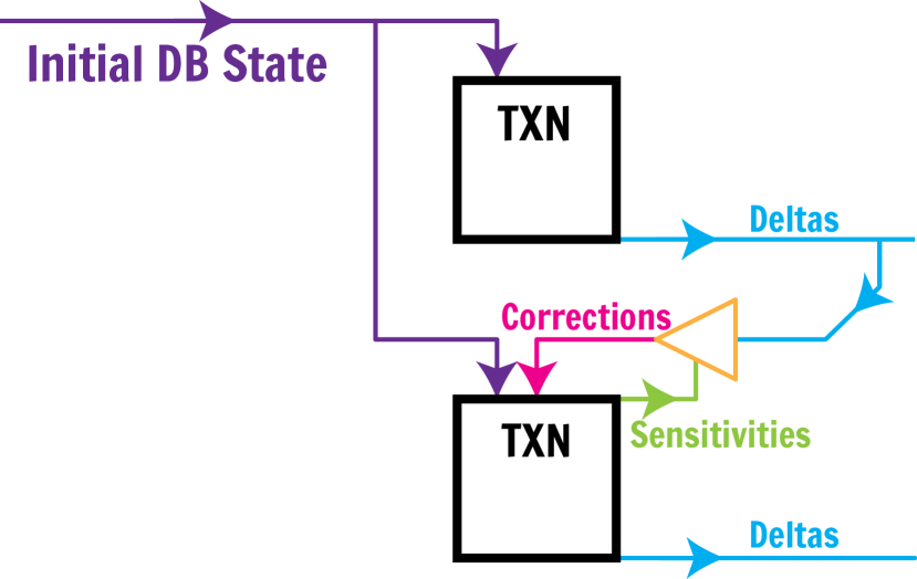
(b) Two transactions run in parallel, with corrections from the first used to repair the second.

Figure 2: Some basic repair circuits.

Suppose there are previous transactions before these two in the serialization order. We need to know what corrections might apply to these two transactions. In Figure 3, we have the first transaction also report its sensitivities; we merge the sensitivities of the two transactions, and add correction circuitry that filters incoming corrections and feeds them back to repair the transactions. To determine the net changes made by the two transactions, we merge their deltas, giving priority to changes made by the second transaction: since it occurs later in the serialized order, its changes supersede those of the first. The merging of the deltas is accomplished by a $\mathsf{merge}$ operator (Section 2.4.2).

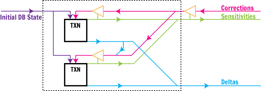
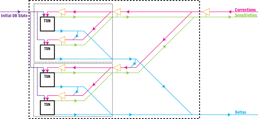
Figure 3: Repair circuits for (a) two and (b) four transactions.

Consider the dotted box of Figure 3. Outside this box we observe the same structure as a single transaction: initial database state and corrections enter the box, and sensitivities and deltas come out. In Figure 3 we duplicate that box of two transactions and wire the boxes as done in Figure 3 for individual transaction boxes. This constructs a transaction repair circuit for four transactions; iterating yields repair circuits for $(2^{k})_{k\in\omega}$ transactions. Each of the dotted boxes of Figure 3 represent a transaction group; individual transactions and groups are arranged in a transaction tree (Section 2.2).

Conceptually, repair circuits are evaluated by fixpoint iteration (Section 3): when inputs to a merge operator, correction operator, or individual transaction change, the circuit element is refreshed, and its outputs are revised as appropriate. For simple transactions, the number of steps required for convergence is controlled by the length of the largest conflict chain. Multiple transactions both reading and writing the same record are a common cause of conflict chains. Figure 4 illustrates a conflict chain among three transactions: the first transaction modifies a record read then written by the fourth transaction; the seventh transaction reads the record. As the fixpoint iteration proceeds, deltas from the first transaction are routed as a correction to the next transaction in the conflict chain, and its deltas will be routed to the next transaction in the conflict chain, until all the conflicts are resolved and the combined deltas are consistent with serial execution.

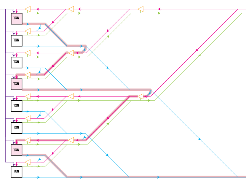
Figure 4: A conflict chain of three transactions. Deltas from the first transaction are propagated as corrections to the fourth, and deltas from the fourth are propagated as corrections to the seventh transaction.

The repair circuit diagrams expose parallelism in an obvious way: multiple cpus can be simultaneously evaluating and repairing transactions, and computing merges and corrections. We need not limit ourselves to multiple cores. If transaction arrivals exceed the capacity of a single machine, we can scale out to clusters: label the outermost box of Figure 3 ‘machine 0’; repeating the earlier constructions we obtain a repair circuit for four machines (Figure 5). The signal lines carrying deltas, sensitivities, and corrections become communications between machines. In this diagram we have omitted correction and sensitivity signals that would be unnecessary, assuming machine 0 contains the first transactions in a commit group.

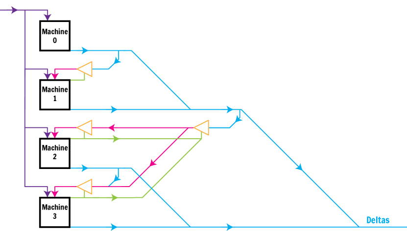
Figure 5: Communication circuit for transaction repair on a four-machine cluster.

2 Repair circuits in depth

We now describe repair circuits in depth.

For simplicity, the exposition of Section 1.4 omitted a major detail. From Figure 3 one might construe that the largest dotted box emits a single signal containing changes from four transactions, and in general the work performed by top-level merge operators is proportional to the number of transactions. This is not the case.

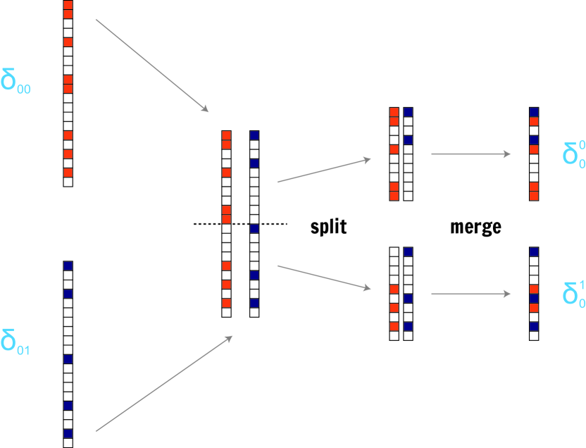
Figure 6: Operation of a merge operator. Delta signals $\delta_{00},\delta_{01}$ from two transactions are partitioned into subdomains at a split point. Delta records below the split point are placed in $\delta_{0}^{0}$, and the others in $\delta_{0}^{1}$.

To better expose parallelism, when we merge delta signals, we simultaneously perform a domain split, separating the merged deltas into those for two disjoint subdomains. Figure 6 illustrates the merge of two delta signals $\delta_{00},\delta_{01}$. The subscripts are a binary representation of the transaction label (zero and one in a group of four transactions), indicating the order of transactions in the serialization order. Records describing changes to the first half of the domain are placed in a signal $\delta_{0}^{0}$, and the remainder are placed in $\delta_{0}^{1}$. The subscript $0$ of these signals labels the transaction group; a group with label $t$ contains all transactions whose label begins with the prefix $t$. The superscript labels the domain split: the two halves of the domain are given subdomain labels $0$ and $1$, and when split into quarters the subdomains would be labelled $00$, $01$, $10$, and $11$. We will refer to subdomain labels using the letter $d$, and transaction group labels using the letter $t$. A merge operator for deltas always takes a pair of signals of the form $\delta_{t0}^{d}$ and $\delta_{t1}^{d}$, which carry deltas in a subdomain $d$ for two sibling transaction groups $t0$ and $t1$, and emits a pair of signals with form $\delta_{t}^{d0}$ and $\delta_{t}^{d1}$: these are deltas for the two halves of the subdomain $d$ (namely, $d0$ and $d1$) for the entire group of transactions $t$ (which contains all transactions in groups $t0$ and $t1$).

Figure 7 shows the detailed wiring of delta and sensitivity signals for a group of four transactions. The four delta signals emitted by individual transactions are merged into four delta signals, each corresponding to a quarter of the domain. Merging of sensitivity signals is similar to that of delta signals, with modest adjustments (Section 2.4.2.)

2.1 Domains and subdomains

We now define the domain. In brief, all tuples in the database can (conceptually) be placed in one set $D$ with a natural total order $(D,\leq)$. We specify subdomains of the database as intervals $[d_{1},d_{2})$ where $d_{1},d_{2}\in D$. Tuples of $D$ have form $(P,\overline{k})$, where $P$ is a relation or function symbol, and $\overline{k}$ is a key tuple. In practice fixed-width identifiers (e.g. integers) can be used to label predicates. Readers content with this synopsis of $D$ may skip to the next heading, bypassing some mildly belabored definitions.

The LogicBlox database engine implements a key-value store with set semantics. A database instance has much in common with a structure of (many-sorted) first-order logic. A database schema defines function symbols $F_{0}$, $F_{1}$, $\ldots$, $F_{m}$ and relation symbols $R_{0}$, $R_{1}$, $\ldots$, $R_{n}$, each with an associated signature specifying key and value arities, and types. (For example, $F[\mathsf{int}$, $\mathsf{string}]=\mathsf{decimal}$ specifies a function with key-arity 2 and value-arity 1.) A nullary function (with key arity 0) is a scalar; relations always have value arity 0. Each type $T$ has an associated total order $(T,\leq_{T})$ predefined and/or dynamically maintained by the database engine.

We refer to functions and relations as predicates. For most purposes of this paper, a predicate symbol $P$ has an associated data structure representing the elements of $P$. (Predicate symbols can also represent primitives such as integer addition, multiplication, etc.; these are largely irrelevant to our purpose, apart from a brief mention in Section 4.)

For each predicate P, let $T_{P}=T_{1}\times\ldots T_{k}$, where $T_{1},\ldots,T_{k}$ are the key types of its signature, and let $(T_{P},\leq_{T_{P}})$ be the lexicographical order on tuples. The data structure for a predicate $P$ provides $O(\log|P|)$ lookups, and $O(1)$ amortized iteration of elements in the order $\leq_{T_{P}}$.

Finally, we define the domain $D$ by:

$$D \equiv\{+\infty,-\infty\}\cup\left(\bigcup_{P}\{P\}\times T_{P}\right)$$ (1)

where $\pm\infty$ are endpoints of the domain, and $\bigcup_{P}\cdot$ ranges over function and relation symbols. Elements of $D$ other than $\pm\infty$ are of the form $(P,\overline{k})$, where $P$ is a predicate symbol, and $\overline{k}$ is a key tuple. Fix an arbitrary order on predicate symbols, and define a total order $(D,\leq_{D})$ where $\pm\infty$ are the endpoints, and lexicographical order on elements of the form $(P,\overline{k})$: tuples ordered first by predicate symbol, and secondarily by key order within each predicate. Subdomains can then be specified as intervals $[d_{1},d_{2})$, where $d_{1},d_{2}\in D$.

2.1.1 Domain decomposition

A domain decomposition is specified by a binary tree, each node labelled by a tuple $s\in D$ of the form $(P,\overline{k})$, $P$ being a predicate symbol. The tuple $s$ is a split point. The root node of the tree is associated with the subdomain $[-\infty,+\infty)$ of $D$. A root node with split point $s$ has a left child ssociated with the subdomain $[-\infty,s)$ and a right child with $[s,+\infty)$; and so on down the tree. We specify a subdomain with a binary string $d\in\{0,1\}^{\ast}$ identifying a tree path, starting from the root and taking left or right branches for 0 or 1, respectively. Split points can be placed between predicate symbols by choosing something with form $(P,[-\infty,\ldots,-\infty])$, or within the records of a predicate.

For exposition it is handy to assume the domain decomposition tree has height $\log_{2}n$, where $n$ is the number of transactions in the repair circuit under discussion. In practice the height and contents of the domain decomposition tree can be tweaked to finesse performance. For example, if there is an influx of microtransactions, one might elect to defer domain splitting until a group of transactions is large enough to warrant it. This can be accomplished by dynamically revising a domain decomposition subtree specifying subdomains $[s_{0},s_{1}),[s_{1},s_{2}),\ldots,[s_{k-1},s_{k})$ into one with subdomains $[s_{0},s_{k}),\emptyset,\ldots,\emptyset$.

2.2 The transaction tree

Individual transactions are arranged in a serialization order, and labelled with binary strings indicating their placement: $000$, $001$, $010$, $\ldots$ $111$ for a group of eight. We’ll say a transaction is later than another if its label is lexicographically greater. We will use the symbol $t$ to represent a transaction label or a prefix of a transaction label.

The transaction tree is a binary tree whose leafs are transactions, and internal nodes are transaction groups. Groups nodes are labelled in the obvious way: a group node with label $t$ has left child $t0$ and possibly a right child $t1$. The leaf positions of the transaction tree are always populated left to right, heap-style. In Figure 7, the transaction tree is implicit in the containment relation of boxes: the outermost box is the root, which contains group 0 and 1; group 0 contains transactions 00,01 and group 1 contains transactions 10,11.

Each transaction node maintains a count of leafs in its subtree, so we can quickly determine whether a subtree can incorporate another incoming transaction (Section 3.2).

2.3 Signals

A signal is an information flow between operators. Signals are realized by data structures; between machines, changes to signals are communicated by protocol. Signal names bear sub- and superscript labels indicating (respectively) their transaction group and subdomain. For example, the signal $\delta_{00}^{010}$ carries deltas from the first (00) transaction (group) that occur in the third (010) subdomain (the first two being, of course, 000 and 001.) Signals are emitted by operators (Section 2.4); each time an operator is refreshed, it emits updates to all of its output signals in a single atomic operation.

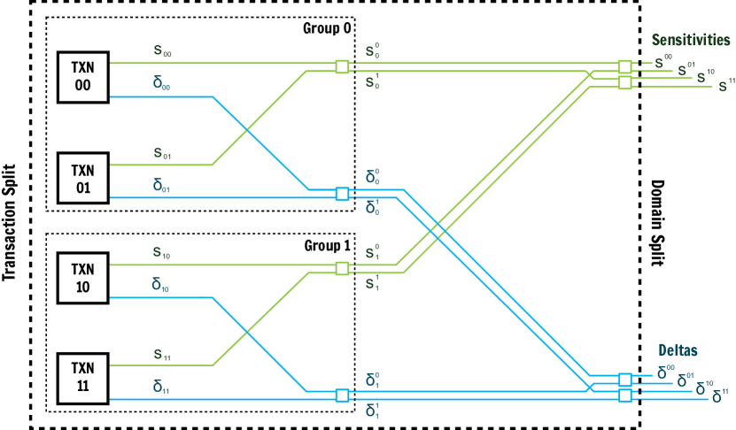
Figure 7: Transaction split and domain split. Small blue boxes indicate $\mathsf{merge}$ operators, and green boxes are $\mathsf{corr}$ (correction) operators.

Delta signals ($\delta_{t}^{d}$) carry changes to database state. Each delta record is of the form $(A,\overline{k},\overline{v},\pm)$, where $A$ identifies a predicate, $\overline{k}$ is a key tuple, $\overline{v}$ is a value tuple, and $\pm\in\{+,-\}$ distinguishes upserts and retractions. An upsert $(A,\overline{k},\overline{v},+)$ indicates the update or insertion of a record (hence the portmanteau). For a relation $R(\overline{k})$, the value tuple $\overline{v}$ is omitted (or construed to be the empty tuple). For a scalar quantity (i.e. a nullary function), $\overline{k}$ is an empty tuple. A retraction $(R,\overline{k},\cdot,-)$ indicates removal of a record; the value tuple is omitted.

Correction signals ($c_{t}^{d}$) also carry changes to database state. They have the same format as delta signals; the name correction distinguishes them as signals carrying relevant deltas back toward transactions in need of repair. (When a delta signal is filtered with sensitivities by a $\mathsf{corr}$ operator, it becomes a correction signal.)

Sensitivity signals ($s_{t}^{d}$) carry information about what aspects of database state might require repairing a transaction, if changed. Each sensitivity record is of the form $(A,[\overline{k}_{1},\overline{k}_{2}])$, where $A$ identifies a predicate, and $[\overline{k}_{1},\overline{k}_{2}]$ is an interval of key tuples. For efficiency, sensitivity records can be represented in the form $(A,\overline{k}_{0},[\overline{k}_{1}^{\prime},\overline{k}_{2}^{\prime}])$, where $\overline{k}_{0}$ is a prefix common to $\overline{k}_{1}$ and $\overline{k}_{2}$, and $\overline{k}_{1}^{\prime},\overline{k}_{2}^{\prime}$ give the remaining tuple elements. This form of sensitivity intervals is emitted by the incremental variant of leapfrog triejoin (Section 4).

2.3.1 Signals associated with transaction nodes

Leaf nodes of the transaction tree have height 0; a group node has height one greater than its children. A tree node (leaf or group) of height $h$ is associated with the following signals:

• $2^{h}$ delta signals, named $\delta_{t}^{0\cdots 000}$, $\delta_{t}^{0\cdots 001}$, $\delta_{t}^{0\cdots 010}$ etc., where the domain labels have $h$ binary digits. (Leaf nodes have empty domain labels.)

• $2^{h}$ sensitivity signals $s_{t}^{0\cdots 00}$, etc.

• $2^{h}$ correction signals $c_{t}^{0\cdots 00}$, etc.

2.3.2 Data structures for signals

A signal can undergo multiple revisions as transactions are repaired. To avoid concurrency hazards, one can either employ read-write locks (i.e. each operator acquires read locks on signals it inputs, and write locks on signals it outputs, and is postponed until such locks can be acquired); or one can use a lock-free, purely functional representation. We have used both in practice, and have a slight preference for purely functional data structures, as they simpler, intrinsically scalable, and adapt easily to repair circuits that span multiple machines.

For efficiency, we want to incrementally maintain operators when changes occur to their signals, rather than evaluating from scratch each time an operator is refreshed. For this reason, signals must support versioning and efficient enumeration of changes between versions: each time a signal is read, it has an associated version-id (an ordinal), and we must be able to enumerate changes between two specified version-ids in time $O(\Delta\log n)$ where $n$ is the number of records in the latest version, and $\Delta$ is the number of update operations (i.e. records inserted or removed) performed between the specified versions. This can be achieved by a variety of purely functional, versioned, or persistent data structures [8, 12]. We employ data structures with efficient iterators that support seeking i.e. $O(m\cdot\log(n/m))$ time to visit $m$ of $n$ records, in order.

2.4 Operators

Signals are processed by operators: each operator inputs a few signals, and outputs one or two signals. An operator tracks the version-id for its inputs, so that each time an operator is refreshed it can efficiently enumerate changes that have occurred to its inputs.

Three operators are employed: $\mathsf{txn}$, $\mathsf{merge}$, and $\mathsf{corr}$. For each, we describe their operation in both full evaluation and incremental maintenance mode.

2.4.1 The txn operator

Each transaction $t$ is implemented by an operator $\mathsf{txn}_{t}$ which reads the database state and corrections $c_{t}$ that reflect relevant updates to the database state by older transactions. A transaction outputs a delta signal $\delta_{t}$ which indicates changes it makes to the database state, and a sensitivities signal $s_{t}$ indicating aspects of the database state it read or attempted to read:

$$\mathsf{txn}_{t}\left(\mathsf{db},c_{t}\right) \Rightarrow(s_{t},\delta_{t})$$ (2)

We describe the details of individual rules and transactions in Sections 4 and 5. In summary, a transaction consists of multiple rules that may query database state and request updates of it. In full evaluation mode, each transaction rule is evaluated. Rule evaluation emits sensitivity records, originating from incremental leapfrog triejoin (4). Some rules may produce deltas (requested changes to database state). In incremental evaluation mode, the transaction is repaired for relevant corrections made to the database state, as carried by the correction signal $c_{t}$ (Section 5).

If an error occurs in a transaction that would require its abort in serial execution (e.g. an integrity constraint failure), the output signals are revised to be empty: $\delta_{t}=\emptyset$, $s_{t}=\emptyset$. The transaction is not officially aborted until all its input signals have been marked as finalized (Section 3.1.4); a failure might be transient, and the transaction might succeed once repaired for changes made by previous transactions.

2.4.2 The merge operator

The $\mathsf{merge}$ operator takes a pair of transaction-split signals and produces a pair of domain-split signals. Merge operators are used to combine delta signals, and to combine sensitivity signals (Figure 7).

For sensitivity signals, a use of the merge operator has the form:

$$\mathsf{merge}\left(\left[\begin{array}[]{c}s_{t0}^{d}\\ s_{t1}^{d}\end{array}\right]\right) \Rightarrow\left[\begin{array}[]{c}s_{t}^{d0}\\ s_{t}^{d1}\end{array}\right]$$ (7)

When a merge operator is constructed, it is given a split point of the form $(R,\overline{k})$, where $R$ identifies a database relation, and $\overline{k}$ is a key tuple (Section 2.1.1). Each sensitivity record represents an interval (Section 2.3). Records whose key interval endpoint is $<\overline{k}$ are placed in $s_{t}^{d0}$, and those whose interval start is $\geq\overline{k}$ are placed in $s_{t}^{d1}$. If a sensitivity record $(R,[\overline{k}_{1},\overline{k}_{2}])$ straddles the split point, two records are emitted: $(R,[\overline{k}_{1},\overline{k}])$ is placed in $s_{t}^{d0}$, and $(R,[\overline{k},\overline{k}_{2}])$ is placed in $s_{t}^{d1}$. Sensitivity records from the two transaction subtrees may overlap; one can eliminate duplicates, merge overlapping intervals, and so forth.

The merge operator for delta signals is simpler. Delta signals carry records of the form $(R,\overline{k}^{\prime},\overline{v},\pm)$; records with $\overline{k}^{\prime}<\overline{k}$ (below the split point) are placed in $\delta_{t}^{d0}$, and those with $\overline{k}^{\prime}\geq\overline{k}$ are placed in $\delta_{t}^{d1}$. When a record for a key $\overline{k}^{\prime}$ occurs in both $\delta_{t0}^{d}$ and $\delta_{t1}^{d}$, the delta from $\delta_{t1}^{d}$ is given priority, since it originated from a later transaction. Note that when $\delta_{t0}^{d}$ contains an upsert record $(R,\overline{k},\overline{v},+)$ and $\delta_{t1}^{d}$ contains a retraction record $(R,\overline{k}^{\prime},\cdot,-)$, the retraction record is emitted; the retraction and insertion do not annihilate.

Full evaluation: using a pair of iterators for the incoming signals, one can iterate the records in order, and write corresponding record(s) to the outgoing subdomain signals as described above. If an identical record occurs in both input signals, only one instance need be emitted.

Incremental evaluation: for each changed record, revisit the merge for that record, revising the output signal appropriately.

2.4.3 The corr operator

Conceptually, the $\mathsf{corr}$ filter is responsible for intersecting a sensitivity signal with delta and correction signals, propagating relevant corrections toward transactions in need of repair.

$$\mathsf{corr}\left(s_{t0}^{d},[c_{t}^{d0},c_{t}^{d1}],\emptyset\right) \Rightarrow c^{d}_{t0}$$ (8)

$$\mathsf{corr}\left(s_{t1}^{d},[c_{t}^{d0},c_{t}^{d1}],\delta_{t}^{d0}\right) \Rightarrow c^{d}_{t1}$$ (9)

Each $\mathsf{corr}$ operator takes a sensitivity signal, a pair of domain-split correction signals, and an optional delta signal. (The delta signal is used for right children of transaction nodes, but not for left children.)

In full evaluation mode, one can choose among multiple strategies, basing the decision on whether there are many sensitivities and few corrections/deltas, or vice versa; one can choose a different strategy for each predicate P mentioned in the signals. In all cases, records from the delta signal supersede those of the correction signal, since they originate from later transactions.

1. If there are comparatively few sensitivity records, one can iterate the sensitivity records of $s^{d}_{t1}$. For each sensitivity record, extract from $\delta_{t}^{d0},c_{t}^{d0},c_{t}^{d1}$ all record(s) which intersect.

2. If there are many sensitivity records, and comparably few corrections and deltas, one can iterate the corrections and deltas, and for each record look for a sensitivity record with a containing interval. Special data structure support is required, as is done for incremental leapfrog triejoin (Section 4.1). Only one matching sensitivity interval is required; one need not find all matching intervals, as in incremental leapfrog triejoin.

Incremental evaluation:

1. If the sensitivity signal is unchanged since the last refresh: For each of $\delta_{t}^{d0},c_{t}^{d0},c_{t}^{d1}$, enumerate the changes since the last refresh, collecting key tuples in a priority queue. Iterate through these keys in order. For each key, determine the net change (for example, an record might be removed from $c_{t}^{d0}$ but also inserted to $\delta_{t}^{d0}$, a net insertion. For removed records, remove them from the output signal, if present. For inserted records, search for a matching sensitivity interval, as in strategy(2) above.

2. If the sensitivity signal has changed, but the correction and delta signals have not, iterate changes to the sensitivity signal, and use iterators for $\delta_{t}^{d0},c_{t}^{d0},c_{t}^{d1}$ to efficiently seek matching records. For inserted sensitivity intervals, matching records are placed in the outgoingcorrection signal. For removed sensitivity intervals, one must determine whether a matching sensitivity interval still exists for each correction/delta record contained in the removed interval. (Alternately, one can maintain a count of the number of matching sensitivity intervals for each correction/delta, and remove a correction/delta when its count reaches zero.)

3. If both the sensitivity signal and one or more of the delta & sensitivity signals have changed, apply both (1) and (2), using the previous version of the sensitivity signal in (1), and then the newer version of all signals in (2).

2.5 Summary of wiring

The following equations summarize the operators and signals of a repair circuit.

$$\mathsf{txn}_{t}\left(\mathsf{db},c_{t}\right) \Rightarrow(s_{t},\delta_{t})$$ (10)

$$\mathsf{merge}\left(\left[\begin{array}[]{c}\delta_{t0}^{d}\\ \delta_{t1}^{d}\end{array}\right]\right) \Rightarrow\left[\begin{array}[]{c}\delta_{t}^{d0}\\ \delta_{t}^{d1}\end{array}\right]$$ (15)

$$\mathsf{merge}\left(\left[\begin{array}[]{c}s_{t0}^{d}\\ s_{t1}^{d}\end{array}\right]\right) \Rightarrow\left[\begin{array}[]{c}s_{t}^{d0}\\ s_{t}^{d1}\end{array}\right]$$ (20)

$$\mathsf{corr}\left(s_{t0}^{d},[c_{t}^{d0},c_{t}^{d1}],\emptyset\right) \Rightarrow c^{d}_{t0}$$ (21)

$$\mathsf{corr}\left(s_{t1}^{d},[c_{t}^{d0},c_{t}^{d1}],\delta_{t}^{d0}\right) \Rightarrow c^{d}_{t1}$$ (22)

1. For each transaction leaf node, we instantiate the transaction operator Eqn. (10).

2. At each transaction tree group node $t$ of height $h$, we instantiate $\mathsf{merge}$ and $\mathsf{corr}$ equations for all $2^{h}$ binary strings $d$ of length $h$, e.g., for height h=3 we would use $d\in\{000$, $001$, $010$, $\ldots$, $111\}$.

3 Transaction repair in action

3.1 Fixpoint mechanics

Conceptually, the transaction repair circuit is evaluated using a fixpoint iteration. A naive iteration would initially set all signals (apart from initial database state) to $\emptyset$. In the first iteration one would evaluate every operator; in subsequent iterations, refreshing only operators whose input signals changed in the previous iteration.

Time can be saved by using an appropriate relaxation of the iteration schedule. In a relaxed schedule, we do not refresh operators in a lockstep global fixpoint iteration, but rather refresh individual operators opportunistically and in parallel with no fixed schedule; each time a compute unit becomes available, we select an operator for it to refresh. In addition, we require that each operator be selected for refresh at least once, and an operator with a changed input must eventually be refreshed. This style of fixpoint evaluation is known as an asynchronous (or chaotic) relaxation.

3.1.1 Soundness and convergence

An obvious concern is whether asynchronous relaxation is sound and convergent for transaction repair. We make an informal convergence argument by induction over the serialization order. The convergence is to a unique fixpoint, hence sound. The argument relies on some assumptions:

1. The database is finite.

2. Operators are purely functional, i.e., their output signals are uniquely determined by their input signals.

3. The evaluation (full or incremental) of an operator always terminates. (For individual transactions, this is enforced by the PTIME bound of our language.)

4. We force the outgoing sensitivity signals of individual transactions to be monotone by never removing records from them. A transaction can contain rules that would otherwise result in nonmonotone updates to the sensitivity signal. For example, a transaction could examine a record $E(10)$ only when a record $D(10)$ is absent; a correction signal bringing the news that $D(10)$ is present would result in the sensitivities decreasing. This makes it challenging if not impossible to fashion a convergence argument. We therefore require the sensitivity signal from a transaction to be increasing. Since sensitivity signals from individual transactions are monotone, all sensitivity signals in the circuit are, since they are collations of single-transaction sensitivities.

5. We assume individual operators correctly implement their functionality. For example, if we iterate a single $\mathsf{txn}$ operator until it reaches a fixed point (holding the incoming corrections constant), then no subsequent changes made to the incoming corrections outside its reported sensitivity regions will affect it.

We proceed by induction over the serialization order. For the base case: since transaction 0 depends only on the initial database state, which is fixed for the course of the iteration, it will reach its final state the first time it is refreshed.

Induction step: by design, information carried by correction and delta signals flows strictly forward, following the serialization order: no information flows from transaction $j$ to transaction $i$ when $i<j$. If all transactions $<i$ have converged, then delta, sensitivity and correction signals depending solely on transactions $<i$ will converge, as every cycle of such signals is interrupted by a transaction $<i$, whose output signals have converged.

We encounter a slight wrinkle in arguing that transaction $i+1$ will converge. This transaction receives a correction signal from transactions $<i$, and possibly a delta signal from transaction $i$; these signals are modulated by the sensitivity signal emitted by transaction $i+1$ itself (Figure 3, with the top transaction mentally labelled $i$). Here we invoke the enforced monotonicity of the sensitivity signal and finiteness of the database: the sensitivity signal for transaction $i+1$ must eventually converge, since its lattice is finite. Once its sensitivity signal convergences, the convergence of transaction $i+1$ follows by the purely functional operator property.

3.1.2 Priorities

In asynchronous relaxation, it is useful to define a priority on operators. When a compute unit becomes available, we select the operator of highest priority in need of refresh.

The importance of selecting priorities wisely is best illustrated by a bad choice: suppose we gave transactions latest in the serialization highest priority. If we had transactions numbered $0,\ldots,k-1$, each incrementing the same scalar counter, the order of transaction refreshes would be $k-1$, then $k-2,k-1$, then $k-3,k-2,k-1$, etc. i.e. $\Theta(k^{2})$ transaction repairs. Similarly bad things happen if operators at height $h$ of the transaction tree are given priority over those at height $h-1$.

We assign priorities according to the following principles:

1. Transactions are given priorities reflecting the serialization order, with the earliest transaction given highest priority.

2. We label each signal with the priority of the operator generating it. We then assign priority to operators to be lower than their inputs. This encourages operators to wait until all their inputs have converged. Since every signal-cycle contains a transaction, and transactions are assigned fixed priorities, this definition of priorities is well-founded.

3. In (2), we select priorities so that signals depending solely on transactions $<i$ have greater priority than transaction $i$.

3.1.3 Enqueuings

We use a priority queue to track operators in need of refresh. Operators are placed in the queue when these events occur:

1. When a new transaction is added to the transaction tree, its $\mathsf{txn}$ operator is enqueued.

2. When an operator is refreshed, it may change some of its output signals. For each changed output signal, all operators reading that signal are enqueued (if they are not already).

3.1.4 Finalization of signals and transactions

We say a transaction is finalized when it has converged in the sense of Section 3.1.1. Tracking which transactions have been finalized plays a central role in the commit mechanics (Section 3.2.3). The first transaction in the serialization order is finalized at completion of its first evaluation; the first transaction never needs to be repaired. A signal is finalized if it is emitted by a finalized operator; an operator is finalized if all its inputs are finalized. Individual transactions are a special case, due to the cycles between transactions, sensitivities, and corrections. A transaction is finalized once (a) all previous transactions in the serialization order are finalized; and (b) no signals participating in a cycle with the transaction are downstream from an operator either being refreshed or in the queue awaiting refresh.

Once a transaction is finalized, we notify its originator that the transaction has been accepted. (The LogicBlox database sends two notifications for transactions: first of acceptance, and then of durable commit and/or replication.)

3.2 Intake and commit of transactions

In practice the transaction repair circuit is being grown and pruned dynamically as new transactions arrive, and finalized transactions are committed. For efficiency, we try to keep the transaction tree small, since there are additional costs with each increase in height of the tree. One way we do this is by pruning transactions after commit (Section 3.2.3). Another is by deferring intake of new transactions. If transactions are balanced in load, then we only need roughly as many transactions in the tree as there are compute units, plus a number of transactions whose processing time is equivalent to the commit pipeline latency.

When new transactions arrive, they are not immediately added to the transaction tree. Instead they are placed in a holding queue. While there, they may be triaged and their placement in the serialization order optimized (Section 6.1).

When a compute unit seeking an operator to refresh finds none eligible, it selects a transaction from the holding queue and moves it into the transaction tree. Transactions are always inserted to the leftmost unoccupied leaf position. If the transaction tree is full, another layer of height is added by creating a new root node whose left child is the current root node (Figure 8, left).

3.2.1 Null transactions

Null transactions can be employed for load balancing, and to accommodate configurations that do not have a number of machines equal to a power of two. Null transactions produce no deltas or sensitivities; their presence in a circuit does not substantially affect performance, if employed thoughtfully. If transactions require uneven amounts of effort, null transactions can be inserted into the serialization order to alter the allocation of transactions. For arbitrary number of machines, one can pad up to the nearest power of two by inserting phantom machines processing null transactions. (This requires adjustments to domain decomposition to ensure load balance.)

3.2.2 Handling long-running transactions

Transactions do not report any deltas or sensitivities until they complete their initial evaluation. This means we can bump long running transaction(s) from a potential commit set and replace them with null transactions.

We can in general bump arbitrary transactions, even those that have already reported deltas and are undergoing repair. We simply replace the transaction with a null transaction (whose empty delta and sensitivity sets will then propagate out, removing the deltas from the bumped transaction). We can then place the transaction in a new position. To avoid discarding all the repair done so far, we can put the transaction on hold until its sensitivities have propagated out to the root level of the transaction tree, and adjusted corrections have flowed back.

3.2.3 Commit mechanics

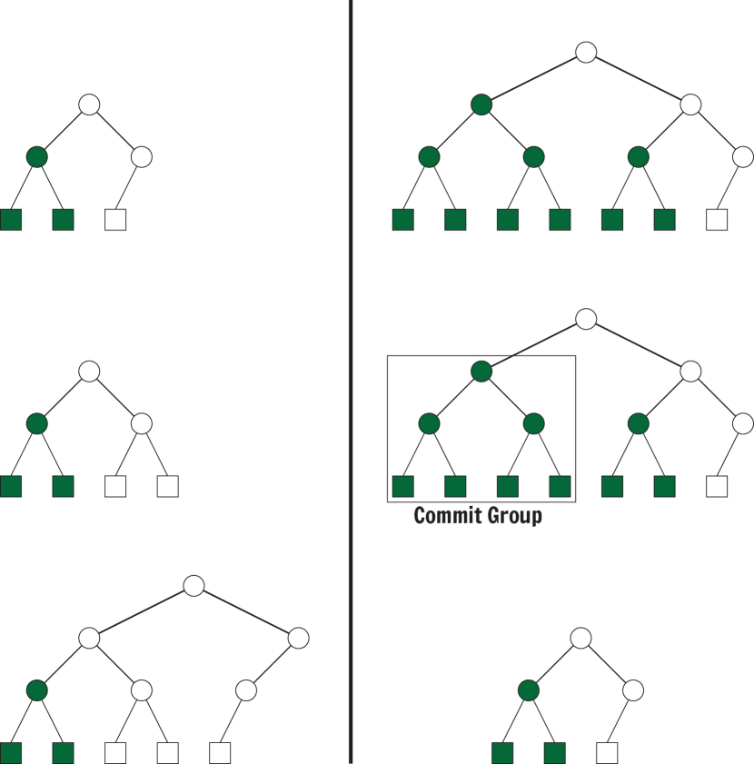
Figure 8: Growing and shrinking the transaction tree. Left, top to bottom: new transactions are placed in the first available leaf position. When the transaction tree becomes full, a new root node is added, with the current tree becoming its left subtree. Right, top to bottom: finalized transactions (and groups) are marked green. The simplest style of commit chooses a finalized left child of the root node (middle). When the left child of the root has been committed, the right child becomes the new transaction tree (bottom).

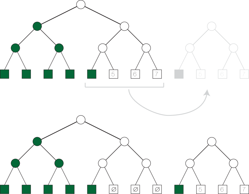
Figure 9: Commit padding. A more ambitious commit can tackle the entire sequence of finalized transactions. The smallest subtree containing all non-finalized transactions becomes the new transaction tree, with finalized transactions replaced by null transactions. Non-finalized transactions in the current transaction tree are replaced with null transactions; once the signals for this tree become finalized, the commit can proceed with the apply-deltas phase.

Our durable commit process is arranged in a somewhat complex pipline, the details of which revolve around particularities of our metadata and page management techniques. The relevant point is that when the first stage of the commit pipeline is idle, it grabs a new batch of transactions and starts them down the pipeline. This batch of transactions is committed as a group, with all members of the group being notified simultaneously when the durable commit and/or replications complete.

There are two strategies that can be employed. The simplest can be used when the root node’s left subtree contains only finalized transactions. In this case we can select the transactions of the left subtree for commit, and place them into the commit pipeline. This strategy is advantageous because the delta signals of the left subtree contain exactly the deltas to be applied to the database state.

Whenever the root node of the transaction tree has a left child whose subtree contains only transactions which have been submitted to the commit pipeline, we discard the left subtree, and the right child of the root node becomes the new root node (Figure 8, right). This discourages the transaction tree from becoming arbitrarily high. (Note though, that signals from the discarded subtree may remain in use by transactions in the tree; they are not garbage collected until they become inaccessible.)

A slightly more complicated strategy can be used to commit all transactions which have been finalized. This involves duplicating the transaction tree, an $O(1)$ operation if purely functional data structures are used. In one version we replace all non-finalized transactions with null transactions, and wait for its top-level delta signals to converge before submitting to the commit pipeline; this ensures no deltas are included from non-finalized transactions. In the other version of the transaction tree, we prune to the smallest subtree containing all nonfinalized transactions (Figure 9).

As the first step in committing a group of finalized transactions, we apply their net deltas to the database state. This can be accomplished by submitting high-priority tasks to the same pool of workers used to refresh operators, with one task for each of the $2^{h}$ subdomains. Each task reads a delta signal for a subdomain, and applies the changes to a branch of the database state. Once all these tasks finish, the branch becomes the new tip version of the database. Transactions arriving after this event are given this new version as their initial database state, and corrections only from the transactions remaining in the tree.

4 Leapfrog Triejoin

In previous sections we have described transaction repair at a high level of detail, with a transaction presented as a black box. In this section and Section 5 we open the box, detailing repair mechanisms at the level of individual transactions.

The LogicBlox database processes transactions that consist of one or more rules written in our LogiQL language, a descendent of Datalog. A simple example of a rule:

$$D(x,y) \leftarrow A(x),B(x,y),C(y).$$ (23)

To the left of the $\leftarrow$ is the rule head listing inferences to be made when satisfying assignments are found for the rule body $A(x),B(x,y),C(y)$. Most rules have straightforward interpretations as sentences of first-order logic:

$$\forall x,y,z~{}.~{}\left[A(x)\wedge B(x,y)\wedge C(y)\right]\rightarrow D(x,y).$$ (24)

The LogiQL language has a rich feature set, but most functionality (in particular, all rule bodies) can be lowered to a minimal core language used by our optimizer and rule evaluators. The syntax of the core language is described by this grammar:

$$\mathsf{rule} ::=\forall\overline{x}~{}.~{}\mathsf{head}\leftarrow\mathsf{conj}$$

$$\mathsf{head} ::=\mathsf{atom}~{}(~{},\mathsf{atom})^{\ast}$$

$$\mathsf{atom} ::=R(\overline{y})~{}|~{}F[\overline{y}]=\overline{z}$$

$$\mathsf{conj} ::=~{}[~{}\exists\overline{x}~{}.~{}~{}]~{}\mathsf{dform}~{}(~{},\mathsf{dform}~{})^{\ast}~{}$$

$$\mathsf{dform} ::=\mathsf{atom}~{}|~{}\mathsf{disj}~{}|~{}\mathsf{negation}$$

$$\mathsf{disj} ::=\mathsf{conj}~{}(~{};\mathsf{conj})^{+}$$

$$\mathsf{negation} ::=\mbox{!}(\mathsf{conj})$$

Atoms can be either relations or functions, and may represent either concrete data structures (representing edb functions/relations, or materialized views), or primitives such as addition and multiplication. Rule bodies must usually adhere to existential ($\exists_{1}$) form, that is, no existential quantifiers under an odd number of negations. User rules not adhering to this form are rewritten by introducing temporary predicates. Sets of rules capture FO+lfp (i.e. PTIME).

We use leapfrog triejoin to enumerate satisfying assignments of rule bodies. Leapfrog triejoin is an algorithm for existential queries that performs well over a variety of workloads, and was recently proven to be worst-case optimal for full conjunctive queries [14]. A few details are pertinent to transaction repair; for a more detailed treatment we refer the reader to [14].

To evaluate a rule such as Eqn. (23), our query optimizer selects an efficient variable ordering for the instance; $[x,y]$, for example. Leapfrog triejoin follows this variable ordering in performing a backtracking search for satisfying assignments: it first looks for $x$ which are present in both $A$ and $B(x,\_)$ (where $B(x,\_)$ is the projection $\{x~{}:~{}\exists y.(x,y)\in B\}$ ). For each such $x$, it searches for $y$ such that $(x,y)\in B$ and $y\in C$.

For each variable a ‘leapfrogging’ of iterators is performed, selecting at each step an iterator and advancing it to a least-upper bound for the positions of the other iterators. Figure 10(a) illustrates this process for $A=\{1,3,4,5,6,7\}$ and $B(x,\_)=\{2,5,7\}$. At $x=5$ all iterators come together on the same value, and the search proceeds to the next variable, $y$ (Figure 10(a), inset box). When values of $y$ satisfying $B(5,y),C(y)$ are encountered, it emits the current variable bindings as a satisfying assignment (e.g. $x=5,y=101$). When one of the iterators reaches its end, the algorithm backtracks to the previous variable, $x$, and continues the search.

4.1 Incremental Leapfrog Triejoin

Leapfrog triejoin admits an efficient incremental evaluation algorithm [13]. For transaction repair this provides a mechanism to quickly repair transaction rules when corrections are made to the database state. The LogicBlox database uses the same incremental evaluation algorithm for efficient fixpoint computation and to maintain IDB predicates, that is, materialized views installed in the database that are kept up-to-date as transactions modify it.

Our incremental evaluation algorithm for leapfrog triejoin is closer to the trace-maintenance style [1] than the approaches typically favoured by the database community [6, 10, 9]. We can view Figure 10(a) as a trace of the leapfrog triejoin algorithm, that is, a fine-grained record of the steps performed in evaluating the rule. By recording a little information about the trace, we are able to efficiently maintain the rule when one of the input relations $A,B,C$ changes.

Consider the operation of the iterator for $C(y)$ in the inset box of Figure 10(a). The last iterator operation for $C$ moves from 104 to 108; this occurs because the iterator for B was positioned at 106, so the C iterator is asked to advance to a least upper bound of 106. How would the trace of this iterator operation change if we removed or inserted elements to $C$? Inserting 105 would have no effect: the iterator would ignore 105 in seeking a least upper bound for 106. Inserting 106 or 107 would change the trace, as would removing 108. In general, when an iterator is asked to seek a least upper bound for a key $k$, it is sensitive to any change in the interval $[k,k^{\prime}]$, where $k^{\prime}$ is the current least upper bound for $k$. The coloured bars of Figure 10(a) indicate these sensitivity intervals.

We collect such intervals in sensitivity indices. For the $C(y)$ relation of this rule, the sensitivity index has form $C_{\mathit{sens}}([y_{1},y_{2}],x)$, where $[y_{1},y_{2}]$ is a sensitivity interval, and $x$ is a context key. For the iterator operation that moves from 104 to 108, the sensitivity index would collect a record $C_{\mathit{sens}}([106,108],5)$. Figure 10(b) shows a sensitivity index for which includes some sensitivity records collected during the search for $y$ with $x=7$ (not shown).

Suppose we modify $C$ by inserting $102$, and we now wish to incrementally maintain the rule. To determine what regions of the trace need revision, we query the sensitivity index to find intervals that overlap the change at $y=102$. We represent sensitivity indices such as $C_{\mathit{sens}}([y_{1},y_{2}],x)$ using a tree that permits rapid computation of prefix sums [5]; its internal nodes are decorated with maximums of interval endpoints $y_{2}$, allowing us to efficiently extract matching intervals. We find a match: $C_{\mathit{sens}}([102,104],5)$, which suggests we revisit the trace where $x=5$ and $102\leq y\leq 104$. Matching sensitivity intervals are used to construct the change oracle, a nonmaterialized view of the union of matching intervals. We then evaluate a special maintenance rule with form:

$$\delta D(x,y,\Delta) \leftarrow\begin{array}[t]{l}(\mathsf{Body}[A,B,C]\cdots\mathsf{Body}[A,B,C^{\prime}])(x,y,\Delta),\\ \mathsf{ChangeOracle}(x,y).\end{array}$$ (27)

where $\delta D(x,y,\Delta)$ is the change in satisfying assignments ($\Delta\in\{+,-\}$), $C^{\prime}$ is the new version of the $C$ predicate,

$$\mathsf{Body}[A,B,C](x,y) \equiv A(x),B(x,y),C(y)$$ (28)

and $(\mathsf{Body}[A,B,C]\cdots\mathsf{Body}[A,B,C^{\prime}])(x,y,\Delta)$ yields the difference between the satisfying assignments of the rule body with the old and new versions of the body predicates. This is implemented by running two leapfrog triejoin algorithms simultaneously, one for the rule body with the old predicates, and one with the new versions. The change oracle restricts evaluation to regions matching sensitivity records. As the maintenance rule (27) is evaluated, we collect sensitivity records from the leapfrog triejoin of the new predicate versions, for use in future maintenance. Figure 11 illustrates the revised trace, with a new satisfying assignment $x=5,y=102$ being found.

Sensitivity records are amenable to compression, conservative approximation, and progressive refinement. In approximating, one can aim for high-fidelity information in volatile regions of the database, and coarser information in static regions, trading accuracy for parsimony to maximize overall performance.

This gives a taste for the incremental version of leapfrog triejoin, used to repair individual rules within a transaction. Issues such as maintaining aggregations, details of the change oracle, etc. are explained in [13].

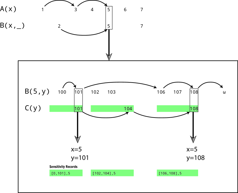
(a) Example of Leapfrog Triejoin in operation (see text).

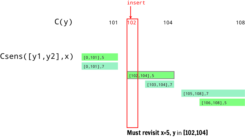
(b) Sensitivity records, some collected from iterator operations in Figure 10(a), and a query for intervals matching $y=102$.

Figure 10: Leapfrog Triejoin.

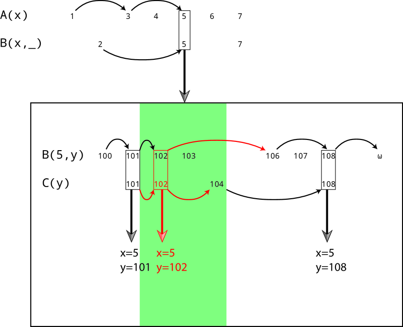
Figure 11: The trace of Figure 10(a) after incremental maintenance for insertion of $C(102)$.

5 Single transaction repair

Setting aside transactions that perform administrative functions, schema changes, install materialized views, etc., for our purposes a transaction is a set of rules to be evaluated. These rules may query database predicates, perform computations using temporary predicates, enforce constraints, and request changes to database predicates. Figure 12(a) shows transaction rules that transfer 100 currency units from Alice’s account to Bob’s account, failing if Alice’s account would be overdrawn. In the head of rule (A) are upserts (^) that request update of $\mathsf{acct\_balance}$ records. The rule body retrieves account numbers for Alice and Bob, and calculates their new account balances. The decoration $\mathsf{@start}$ is used to distinguish the $\mathsf{acct\_balance}$ predicate as it existed at the start of the transaction. The rule (B) is a constraint: if the balance of Alice’s account at the end of the transaction is negative, the transaction fails.

$\displaystyle(A)$ $\displaystyle\begin{array}[t]{l}\mathsf{\textasciicircum acct\_balance}[n_{1}]=a,\\ \mathsf{\textasciicircum acct\_balance}[n_{2}]=b\\ \leftarrow\begin{array}[t]{l}\mathsf{account\_by\_name}[\mathrm{``Alice"}]=n_{1},\\ \mathsf{account\_by\_name}[\mathrm{``Bob"}]=n_{2},\\ a=\mathsf{acct\_balance@start}[n_{1}]-100,\\ b=\mathsf{acct\_balance@start}[n_{2}]+100.\end{array}\end{array}$ $\displaystyle(B)$ $\displaystyle\begin{array}[t]{l}\mathbf{false}\\ \leftarrow\begin{array}[t]{l}\mathsf{account\_by\_name}[\mathrm{``Alice"}]=n_{1},\\ \mathsf{acct\_balance}[n_{1}]<0.\\ {}\end{array}\end{array}$

(a) Two rules of a simple transaction.

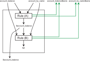
(b) Execution graph for the rules, after some rewriting.

Figure 12: A simple transaction and its execution graph.

The rules are placed in an execution graph. Rules and predicates are vertices; there is an edge $(\mathsf{R},X)$ if predicate $X$ appears in the head of rule $\mathsf{R}$, and an edge $(Y,\mathsf{R})$ if $Y$ appears in the body of $\mathsf{R}$. The rules of Figure 12(b), after some manipulations we describe shortly, result in the execution graph of Figure 12(a). The box indicates transaction scope: database predicates appearing in rule bodies flow into the box, and deltas and sensitivities flow out. Rules reach the execution graph after undergoing several rounds of rewriting. The upserts appearing in the head of rule (A) are rewritten to derive into a delta predicate $\delta\mathsf{account\_balance}[x,\Delta]=y$ containing requested changes, where $\Delta\in\{+,-\}$.

In single-writer operation of the database, we add a frame rule that applies the requested deltas. For transaction repair, transaction rules need adjustment:

• Rather than having a frame rule apply the requested deltas $\delta\mathsf{account\_balance}$ within the transaction scope, we instead emit the deltas from the transaction without modifying $\mathsf{account\_balance}$; these become the delta signal used by transaction repair. Since the body of rule (B) refers to the state of $\mathsf{account\_balance}$ at the end of the transaction, we provide rule (B) a nonmaterialized view with the deltas applied (hence the edge to Rule (B) from $\delta\mathsf{account\_balance}$.) These changes make transactions purely declarative, with no side-effects; mutation of database state only occurs during the apply-deltas phase of the commit process (Section 3.2.3).

• Each rule outputs sensitivity records for its body predicates (Figure 12(b), green). Sensitivity records are stripped of context keys (Section 4.1). Sensitivities are collated at the transaction level, forming the outgoing sensitivity signal used by transaction repair. Records are never removed from the outgoing sensitivity signal, as required for the convergence argument of Section 3.1.1.

• Correction signals from transaction repair are handled by providing database predicates such as $\mathsf{account\_balance}$ and $\mathsf{account\_by\_name}$ to the execution graph as nonmaterialized views that reflect the database predicates after correction. Within a rule, we can access these corrections directly to find matching sensitivity intervals for incremental leapfrog triejoin. In each round of maintenance, we are not looking just at the correction signals, but also changes made to the correction signals.

The rules of Figure 12(b) are implemented as execution units, which expose a simple interface: $\mathsf{beginMaintenance}(\mathbf{P})$ informs an execution unit that a round of maintenance is about to begin, and that revised versions of the predicates named in set $\mathbf{P}$ are to be provided. A revised predicate $P$ is provided by invoking $\mathsf{inputChanged}(\mathsf{name},P)$. Alternatively, one may invoke $\mathsf{inputNotChanged}(P)$. The maintenance round ends with $\mathsf{endMaintenance}()$. Individual rules are maintained using the incremental leapfrog triejoin described in Section 4.1.

The execution graph as a whole also implements the execution unit interface. When input predicates to the graph are revised, we propagate changes through the graph, performing rounds of maintenance on any rules affected, and respecting dependencies. This may result in changes to both the outgoing delta and sensitivity signals for the transaction.

6 Refinements and Variations

We now describe some variations and refinements of transaction repair. These ideas are not yet (as of writing) implemented in our prototype, and hence speculative.

6.1 Selecting serialization orders.

The order in which transactions are placed into the serialization order can have a significant impact on performance. In general the problem falls into the broad category of minimum linear arrangement algorithms [7]. Some of the factors to be considered include:

• Read-only transactions can always be inserted at the very beginning of the serialization order, even when there are already transactions in flight, since their delta signals will always be null. This avoids any repair of read-only transactions.

• If transaction X reads a set of data D, and transaction Y modifies a subset of D, can be advantageous to place X before Y in the serialization order, to avoid repair.

• It is advantageous to group together transactions that read and write similar sets of data in the serialization order. This reduces the need for long sensitivity/correction paths, which will reduce latency cost and improve data locality when merging delta signals.

• Define a conflict graph $G_{C}=(V,E)$ whose vertices are transactions, and there is an edge $(X,Y)$ if the sensitivities of $Y$ intersect the deltas of $X$. Let $G^{\prime}$ be a directed, acyclic subgraph of $G_{C}$, constructed by selecting a subset of transactions $V^{\prime}$ and edges $E\cap V^{\prime}\times V^{\prime}$. Then the transactions $V^{\prime}$ can be placed in a topological order at the start of the serialization order, without requiring any repair. One can use this property by (a) placing new transactions in a triage pool, where they are fully evaluated in isolation (with an empty correction signal) to obtain their initial sensitivities and deltas, and possibly repairing them to keep them up to date with the latest leaf in the transaction tree; (b) building the conflict graph $G_{C}$ for the transactions in the triage pool by determining (or conservatively approximating) conflict edges, and (c) selecting a maximal acyclic subset of vertices $V^{\prime}$ (possibly weighted by transaction cost, or estimated repair cost) to begin a serialization order.

• Randomization may be useful to disrupt linear chains of conflicting transactions. Suppose we have a sequence of transactions $X_{0},\ldots,X_{k-1}$ where $X_{i}$ reads a record $r_{i}$ and writes a (different) record $r_{i+1}$. This creates a conflict chain of length $k$ whose repair could possibly be expensive. Suppose we choose a permutation of $X_{0},\ldots,X_{k-1}$ uniformly at random for our serialization order. The expected length of the longest conflict chain is $2\sqrt{k}$, a substantial reduction; this is an instance of the ‘longest increasing subsequence of a random permutation’ problem posed by Ulam.

6.2 Load balancing techniques

• Microtransactions. If there are large volumes of microtransactions to be proceessed, for example, transactions that read and/or update only a few records, it will be advantageous to group them together as if a single transaction. This can be accomplished by inserting a leaf node into the transaction tree which internally contains multiple transactions arranged in a repair circuit, but without any domain splits being applied. This would defer domain splits until a sufficiently large chunk of deltas and sensitivities have accrued.

• Revising the domain decomposition. In our prototype we have so far used a static domain decomposition. For a system that performs well under varying workloads, one will want to periodically revise the domain decomposition. Ideally this would be done not according to static distribution of data, but according to the intensity of activity, e.g., by using random samples of recent deltas and sensitivities to revise the domain decomposition.

6.3 Trie surgery deltas

Incremental leapfrog triejoin handles trie surgeries in addition to record-level deltas [13]. A trie surgery occurs when the first or last record matching a key prefix is inserted or removed. For some transactions, providing trie surgery deltas will be necessary for performance. To address this, we anticipate maintaining projections of key prefixes, with support counts. When the $\mathsf{merge}$ operator observes a support count making a transition from $0\rightarrow 1$ or $1\rightarrow 0$, it can emit appropriate trie surgery deltas, which can be matched against sensitivities.

6.4 Reducing the cost of sensitivity indices.

Collecting sensitivity information from rules in a transaction introduces some overhead, and propagating sensitivity information through the repair circuit can be expensive. These costs can be reduced by employing heuristics:

• If we can determine statically (i.e. before initial evaluation) that a transaction $X$ reads a set of data D, and no transaction before $X$ modifies $D$, then we do not need to produce sensitivity records from X for D.

• We can trade off the precision vs. parsimony of sensitivity information. If the sensitivity of a transaction is a subset $S\subseteq D$ where $D$ is the domain, then it is sound to use any superset $S^{\prime}\supseteq S$ as the sensitivity information. One could, for example, report sensitivities at the coarse level of page boundaries, or even at the level of entire predicates.

• We can augment the circuit wiring described in Section 2 with what we call sensitivity knockout elements. At each node of the transaction tree, insert an element that uses deltas from the left child to "knock out" sensitivities from the right child. This will avoid artificial dependency chains. For example, in a sequence of transactions that increment a counter, the circuits would include active correction paths from the very first transaction to the last. Knockouts would avoid this: if transaction $2i$ wrote the counter, and $2i+1$ read it, then the sensitivity to the counter of $2i+1$ would be "knocked out" by the delta from transaction $2i$. (This indicates that changes to the counter made by transactions $<2i$ are irrelevant.)

  Knockouts are not necessary within individual transactions (i.e. between rules). If a rule R1 requested an upsert $\mathsf{\textasciicircum}F[\overline{k}]=\overline{v}$, and rule R2 read $F[\overline{k}]$, the reported sensitivity would be to the $\delta F$ predicate emitted by rule R1, not to the $F$ from the database.

6.5 Adaptations for clusters

Transaction repair can be adapted to clusters in a straightforward way. Suppose we have $n$ machines, each with $m$ cores, where both $n,m$ are powers of two. (As mentioned earlier, we can pad the construction with phantom machines and/or phantom cores processing null transactions, to round these numbers up to the nearest power of two.)

Conceptually, we employ a transaction tree of height $\log_{2}(nm)-1$. (If needed, we can expand leaf nodes of the tree to be groups of transactions, and not perform domain splits inside such a group.)

Each of the $n$ machines is labelled by a unique binary string $\in\{0,1\}^{(\log_{2}n)-1}$.

• A signal $\delta_{t}^{d}$ is owned by the machine whose label is a prefix of $td$; similarly for $s_{t}^{d}$ and $c_{t}^{d}$. The operators emitting signals $\delta_{t}^{d}$, $s_{t}^{d}$ and $c_{t}^{d}$ similarly reside on the machine whose label is a prefix of $td$. (There is room for optimizations here; when signals traverse machine boundaries we can consider placing the operators on either of the two machines according to expected performance.) Note that in Figure 7, the merge operators for sensitivities and deltas form an efficient parallel sorting network; for example, all deltas and sensitivities related to the leftmost subdomain are forwarded to the machine with label $000\ldots 0$, and those for the rightmost subdomain are sent to the machine with label $111\ldots 1$.

• If a signal crosses machine boundaries, e.g., it is output by an operator on machine $X$ and input by an operator on machine $Y$, we transmit changes made to the signal from machine $X$ to machine $Y$.

• When the dynamic construction of the repair circuit reaches the last machine, and the last machine’s transaction tree becomes full, we ’wrap around,’ continuing construction of the transaction tree on the first machine. Conceptually, one can imagine transaction operators labelled with $\mathsf{txn}_{et}$, where $t$ is a $\log_{2}(nm)-1$ binary string, and $e$ is a binary string counting the number of times the repair circuit has wrapped around the entire cluster.

• Each machine can accept transactions independently; we relax the left-to-right filling in of the transaction tree, and require this only within each machine. Conceptually one can think of the transaction tree as fully constructed and containing null transactions, which are replaced with real transactions as they arrive.

• Each machine has its own priority queue for operators needing refresh. When updates to signals arrive from other machines, they are treated the same as updates to signals within a machine; any operators reading the signals are added to the priority queue.

• If we use the same domain decomposition for circuits as for dividing responsibility for durable storage of database state, then during the apply-deltas phase of the commit process, each machine has precisely the deltas which apply to the subset of the database for which it is responsible. (Note however, there is a tension here between maintaining a domain decomposition that evenly splits the database contents vs. a decomposition that evenly splits average activity of transactions.)

• The following refinement is conceptually interesting but possibly challenging to make work in practice: suppose that, as mentioned, the same domain decomposition is used for the repair circuit as for responsibility of database state. Each machine provides its transactions with an ‘initial database state’ consisting only of database state currently on the machine (i.e. either state that machine is responsible for, or cached state from other machines). When a transaction attempts to access state unavailable on the machine, the sensitivity signal propagates out to the responsible machine, and the needed state is transmitted back as a correction. This requires some elaboration to be practicable. For example, if a machine has no contents for a predicate $P$, and a transaction has a rule that attempts to read $P$, leapfrog triejoin will typically report a sensitivity for the entire domain of $P$. This would have the unfortunate effect of fetching the entire contents of $P$, even if only a tiny portion of $P$ was required. One way to address this would be to respond gradually to such requests; for example, providing the first few pages of $P$ and waiting for more sensitivity records to be received.

References

- [1] Umut A. Acar, Guy E. Blelloch, Robert Harper, Jorge L. Vittes, and Shan Leung Maverick Woo. Dynamizing static algorithms, with applications to dynamic trees and history independence. In Proceedings of the fifteenth annual ACM-SIAM symposium on Discrete algorithms, SODA ’04, pages 531–540, Philadelphia, PA, USA, 2004. Society for Industrial and Applied Mathematics.
- [2] Philip A. Bernstein and Nathan Goodman. Concurrency control in distributed database systems. ACM Comput. Surv., 13(2):185–221, June 1981.
- [3] Philip A Bernstein and Eric Newcomer. Principles of transaction processing. Morgan Kaufmann, 2009.
- [4] Philip A. Bernstein, Colin W Reid, Ming Wu, and Xinhao Yuan. Optimistic concurrency control by melding trees. Proceedings of the VLDB Endowment, 4(11), 2011.
- [5] Siddhartha Chatterjee, Guy E. Blelloch, and Marco Zagha. Scan primitives for vector computers. In In Proceedings Supercomputing ’90, pages 666–675, 1990.
- [6] Songting Chen. Efficient Incremental View Maintenance for Data Warehousing. PhD thesis, Worcester Polytechnic Institute, 2005.
- [7] Josep Díaz, Jordi Petit, and Maria Serna. A survey of graph layout problems. ACM Comput. Surv., 34(3):313–356, 2002.
- [8] James R. Driscoll, Neil Sarnak, Daniel Dominic Sleator, and Robert Endre Tarjan. Making data structures persistent. In ACM Symposium on Theory of Computing, pages 109–121, 1986.
- [9] Ashish Gupta and Iderpal Singh Mumick. Materialized views: techniques, implementations, and applications. MIT press, 1999.
- [10] Ashish Gupta, Inderpal Singh Mumick, and V. S. Subrahmanian. Maintaining views incrementally. In Peter Buneman and Sushil Jajodia, editors, Proceedings of the 1993 ACM SIGMOD International Conference on Management of Data, SIGMOD ’93, Washington, DC, May 26–28, 1993, volume 22(2) of SIGMOD Record (ACM Special Interest Group on Management of Data), pages 157–166, pub-ACM:adr, 1993. ACM Press.
- [11] Hsiang-Tsung Kung and John T Robinson. On optimistic methods for concurrency control. ACM Transactions on Database Systems (TODS), 6(2):213–226, 1981.
- [12] Chris Okasaki. Purely Functional Data Structures. Cambridge University Press, Cambridge, UK, 1998.
- [13] Todd L. Veldhuizen. Incremental maintenance for leapfrog triejoin. Technical Report LB1202, LogicBlox Inc., 2013. arXiv:1303.5313.
- [14] Todd L. Veldhuizen. Leapfrog triejoin: A simple, worst-case optimal join algorithm. In Proceedings of the International Conference on Database Theory (ICDT), March 2014. arXiv:1210.0481.