Characterization and physical explanation of energetic particles on Planck HFI instrument

Abstract

The Planck High Frequency Instrument (HFI) has been surveying the sky continuously from the second Lagrangian point (L2) between August 2009 and January 2012. It operates with 52 high impedance bolometers cooled at 100mK in a range of frequency between 100 GHz and 1THz with unprecedented sensivity, but strong coupling with cosmic radiation. At L2, the particle flux is about 5 $cm^{-2}s^{-1}$ and is dominated by protons incident on the spacecraft. Protons with an energy above 40MeV can penetrate the focal plane unit box causing two different effects: glitches in the raw data from direct interaction of cosmic rays with detectors (producing a data loss of about 15% at the end of the mission) and thermal drifts in the bolometer plate at 100mK adding non-gaussian noise at frequencies below 0.1Hz. The HFI consortium has made strong efforts in order to correct for this effect on the time ordered data and final Planck maps. This work intends to give a view of the physical explanation of the glitches observed in the HFI instrument in-flight. To reach this goal, we performed several ground-based experiments using protons and $\alpha$ particles to test the impact of particles on the HFI spare bolometers with a better control of the environmental conditions with respect to the in-flight data. We have shown that the dominant part of glitches observed in the data comes from the impact of cosmic rays in the silicon die frame supporting the micro-machinced bolometric detectors propagating energy mainly by ballistic phonons and by thermal diffusion. The implications of these results for future satellite missions will be discussed.

1 Introduction

Planck¹ is a project of the European Space Agency (ESA) with instruments provided by two scientific consortia funded by ESA member states (in particular the lead countries France and Italy), with contributions from NASA(USA) and telescope reflectors provided by a collaboration between ESA and a scientific consortium led and funded by Denmark. It comprises a telescope, two instruments High Frequency Instrument HFI and Low frequency Instrument LFI and a Spacecraft. The High Frequency Instrument (HFI) ³ has be operating with 52 high impedance spiderweb bolometers cooled at 100mK in a range of frequency between 100GHz and 1THz. During the mission the HFI instrument has shown a sensitivity in agreement with requirements but at the same time a strong coupling with cosmic radiation.

Cosmic rays (CRs) ^{7, 8} at Lagrangian point L2 are essentially composed by massive particles: about 89% of protons, 10% of alpha particles, 1% are the nuclei of heavier elements and less than 1% of electrons like beta particles. The total flux of CRs peaks around 200 MeV, giving a total proton flux of 3000 - 4000 particles m^-2 sr^-1 s^-1 GeV^-1. The flux is dominated by galactic CRs which dominates in period of low solar activity. The solar wind decelerates the incoming particles and blocks some of the particles with energies below about 1 GeV. Since the amount of solar wind is not constant due to changes in solar activity, the level of the cosmic ray flux varies with time. This is monitored in Planck satellite by the Standard Radiation Environment Monitor (SREM). The period following the Planck launch was a period of exceptionally low solar activity, resulting in very weak solar modulation of cosmic rays at 1AU⁷. The flux of low energy ($200MeVnucleon^{-1}$) nuclei from carbon to iron was four times higher than in the period between 2001 and 2003, and 20% higher than in previous solar minima over the last 40 years.

In this paper, first we discuss briefly the characteristic of the HFI high impedance bolometers. In section 3 we describe the impact of the cosmic ray in the in-flight HFI data. In section 4 we give the results obtained from ground-based tests which permitted to understand the origins of the different families of the in-flight glitches.

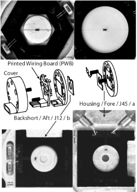
Figure 1: Top: SpiderWeb Bolometer (SWB) with the sensitive NTD thermometer on the centre of the spider absorber (zoom of the absorber and the NTD on top right picture.). Middle: exploded view of a typical HFI bolometer module. Bottom: Polarization Sensitive Bolometer (PSB). Two PSBs are mounted to the same bolometer module. The two pictures show the forward/upper PSBs (PSBb and PSBa).

2 HFI Bolometers

The HFI bolometers are made of a Neutron Transmutation Doped thermistor 30 $\mu$m (thickness) $\times$ 100 $\mu$m $\times$ 350 $\mu$m identical for all these detectors, a free standing metallized $Si_{3}N_{4}$ micromesh supported by $Si_{3}N_{4}$ beams (thickness 1 $\mu$m) and a silicon die. Other elements that composes a bolometer module have no impact on the goals of this paper so they are not discussed here. Details can be found in Holmes et al, 2008¹⁰.

For SWB detectors (spiderweb bolometer, non-sensitive to polarization), the thermometer is at the center of the grid while for PSB detectors (polarization sensitive bolometer) the thermometer is at the edge of the grid as it can be seen on Fig 1. The grid geometry has been chosen so that it absorbs mm-waves with high efficiency but has a much smaller physical surface area reducing significantly the cross section to cosmic ray particles and shorter wavelength photons.

The Silicon die thickness is equal to 350 $\mu$m, common to all the bolometers and the surface area is between 0.4 and 0.8 cm² depending on the working frequency.

3 HFI glitchology

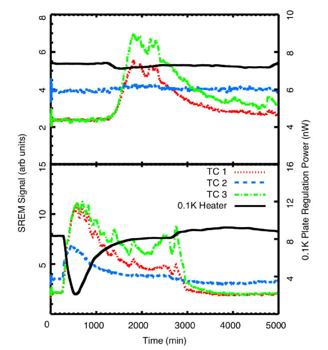
Figure 2: Output of SREM diodes D1, D2 and D3 (left axis) and temperature control heater power on the 0.1K plate (right axis) and as a function of time for large solar flares on March 7 (top) and August 4 (bottom) in 2011.

3.1 The Standard Radiation Environment Monitor

The flux of CRs is monitored onboard the satellite by the Standard Radiation Environment Monitor (SREM) mounted on the exterior of the Planck spacecraft. SREM consists of three detectors (Diodes D1, D2, D3) in two detector head configurations ⁹. A total of 15 discriminator levels are available to bin the energy of the detected events. Solar flares provided a useful test to correlate the signal measured on the out-side of the spacecraft with the SREM to signals due to particle impact on HFI.

During a solar flare the glitch rate increases and the heater power used to regulate the 0.1K cryogenic stage decreases with the increasing deposited power by the particle flux. In Fig 2 the signal of the three different SREM diodes and the temperature control heater on 0.1K cryogenic stage for two large solar flares is shown.

The signals of the heater power and D2 are similar to each other in each flare. However, the peak signal of each is very different comparing the two flares. In addition, there is structure in the signal for D1 and D3 that are not in D2 or the heater power response. We find that this correlation holds between the heater power and D2 for all flares. The diode D2 has the most shielding of the 3 diodes in the SREM, 1.7 mm of Aluminum and 0.7 mm of Tantalum which allows only only ions and protons with energies $>39$ MeV to pass. The other diodes are shielded by 0.7 mm of Aluminum for D3 and 1.7 mm of Aluminum for D1. This demonstrates that the spacecraft and instrument surrounding the bolometers shield particles with energies at least up to 39 MeV and all solar electrons. This is equivalent to the stopping power of $\sim 1.5$ cm of Aluminum.

3.2 Indirect Effect on detectors

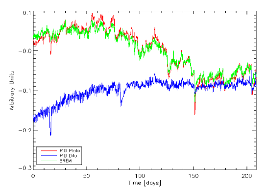
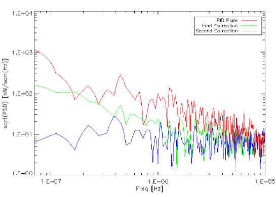
Figure 3: Left: correlation between the signal of the SREM (red) and the signal of the active regulation of the temperature of the bolometer plate. Right: corrected data by subtraction of the SREM (first) and dilution fluctuation signal (second).

The very good correlation between the 100mK stage control heater² and the SREM is shown in Fig 3 left. The correlation with the control heater of the temperature of the dilution plate is smaller. Fig 3 right shows the correction performed by subtracting the data with the SREM (particle contribution) and the fluctuations of the dilution stage (cryogenic contribution). These corrections demonstrate that we have identified all the source of fluctuation in the range of frequencies between 10^-7 and 10^-5 Hz. In flight, the 100mK temperature fluctuations induced by the modulation of Galactic cosmic rays dominate, but they do not affect the signal. In the frequency range between 16 mHz and 300 mHz, excess noise from cosmic rays with respect to ground measurements is seen on the bolometers and thermometers; however, any common thermal mode affecting all thermometers and bolometers that is not fully corrected by the bolometer plate control heaters is removed using the dark bolometer signals. After corrections we find a flat noise spectrum in agreement with the one obtained from ground calibrations².

Another source of 100mK plate temperature fluctuation is showers of particles resulting from interaction of very high energy particles with the payload. The rate of these event is about one per day. Showers of particles deposit energy in the 100mK plate but also directly in the detectors. these events are not discussed in this paper. For a detailed discussion see the LTD-15 Miniussi proceeding.

3.3 Direct effect on detectors

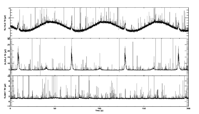
Figure 4: Raw TOIs for three bolometers, 143GHz (top), 545GHz (middle), and a Dark1 bolometer (bottom) illustrating the typical behaviour of a detector at 143 GHz, 545 GHz, and a blind detector over the course of three rotations of the spacecraft at 1 rpm. At 143 GHz, one clearly sees the CMB dipole with a 60 s period. The 143 and 545GHz bolometers show vividly the two Galactic Plane crossings, also with 60 s periodicity. The dark bolometer exhibits a nearly constant baseline together with a population of glitches from cosmic rays similar to those seen in the two upper panels. The typical maximum amplitude of a spike is between 100 and 500 mV depending on the bolometer.

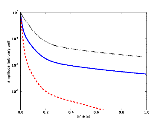
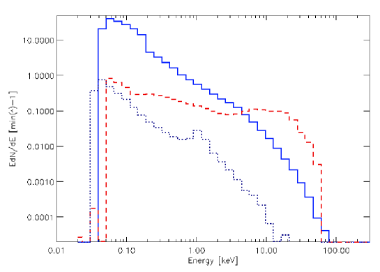
Figure 5: Left: average short glitch template (red dashed curve), long glitch template (blue solid curve) and slow glitch template (dotted black curve) in the case of one PSB in- flight bolometer. Right: glitch energy distribution of the glitches observed by HFI in-flight for short (dashed red), long (solid blue) and slow (dotted black) in the case of one PSB in-flight bolometer; the x-axis represents the absorbed energy in the NTD.

Glitches in raw data result from the direct impact of cosmic rays in the bolometer module. In Fig 4 we present the raw data for three HFI detectors showing that the rate is quite conspicious (about 2 per second).

The collaboration has identified three types of glitches with different shapes. The fitted templates and the spectra of these short, long and slow types of glitch are drawn in Fig 5.

Short glitches present a fast decay (between 4 – 10 ms depending on the bolometer) and a tail with an amplitude of fews percentage points relative to the largest amplitude. The tail shows intermediate time constants of the order of tens of ms and a third time constant of about 1 s with a relative amplitude of 0.1 %. Long glitches present the same fast decay as the short ones but a large (about 10 %) relative amplitude tail showing intermediate to long time constants of tens of ms and a third time constant of about 1 s with a relative amplitude of 0.1 %. Slow glitches show the same slow time constants but not the fast decay; they are present only in the foward PSB (in Planck focal plane PSBs are arranged in pairs sensitive to orthogonally-oriented polarization).

Slow and long glitch spectra exhibit similar shapes, so they should share some parts of the of the energy deposition process. Long glitch spectra have a plateau below 1 keV followed by a power-like spectrum and a smooth cut from about few hundreds of keV to 1 MeV. Short glitch spectra have a double structure with a power-law below 10 keV followed by a bump very similar for all bolometers (except 857 GHz ones) and then few events above 100 keV (around one per day). Very high energy events are rare but we have enough statistics to see such unprobable signals due to cosmic ray crossing the grid along a line.

4 The origin of the excess HFI glitches : ground tests

For an improved understanding of the origins of the glitches ¹¹ seen in HFI flight data, we performed several ground-based tests on HFI spare bolometers between the late 2010 and spring 2013. The aim of the tests is to have a more complete view of the physical explanation of the different families of glitches. These tests have been performed in different configurations using 23 MeV protons from a TANDEM accelerator and two radioactive $\alpha$ particle sources (²⁴¹Am, ²⁴⁴Cm and X-rays ⁵⁵Fe to calibrate the signal). The list of all the performed tests with the main characteristics of the setup is presented in Table 1.

	TANDEM acc. Tests	$\alpha$ Test 1	$\alpha$ Test 2
Place	IPN - Un. of Paris-sud	Neel Institute - Grenoble	IAS - Un. of Paris-sud
Period	Dec. 2010	Nov. 2011–Apr. 2013	June–Nov. 2011
Source	TANDEM accelerator	${}^{55}Fe$ isotope source	${}^{241}Am$ Source
	$p^{+}$ at 23 MeV	(X-rays 5.4 keV, 1.3 kBq	($\alpha$ particles at 5.4 MeV,
		produced in 2006)	3 Bq)
		${}^{244}Cm$ Source
		($\alpha$ particles at 5.9 MeV, about 1kBq)
Cryostat	Néel 100 mK dilution	Néel 100 mK dilution	IAS 100mK dilution
Detectors	3 SWB	1 SWB - 1 PSB	1 SWB - 1 PSB
Read-Out El.	AC biased (Same as HFI)	AC biased (Same as HFI)	DC (dig. at 5 kHz)

Table 1: List of all the performed tests with the principal characteristics of the setup.

5 Interpretation

5.1 Short glitches origin

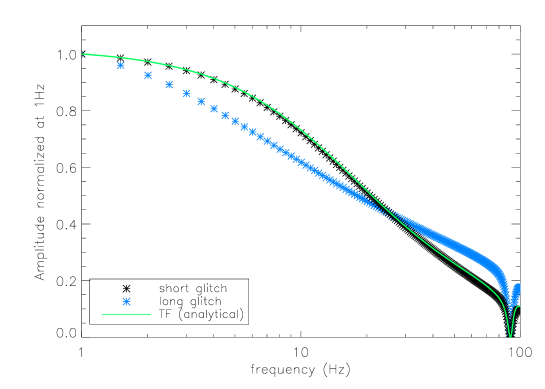
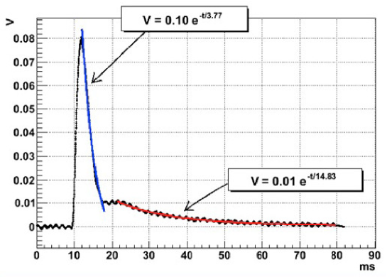
Figure 6: Left: Comparison of the HFI Optical transfer function³ (solid green), short glitch templates (black stars) and long glitch template (blues stars). Right: glitch template built by stacking 466 events coming from impacts in the silicon wafer.

There is clear evidence that the short events are resulting from cosmic rays hitting the grid or the thermistor. Indeed, those events have a fast rising time and have a fast decay, and the transfer function (Fig 6 left) built from the short glitch template is in good agreement with the HFI optical transfer function, so the energy must be deposited in the environment close to the thermistor. The energy distribution of the short glitches is very stable between bolometers and the data show a double structure⁴. The bump of the short glitch distribution, centred at about 20 keV, is completely consistent with the interaction between CRs and the NTD thermometer. In the low energy regime, the distribution corresponds to the interaction between the absorber and the CRs. For PSB bolometers, the level of PSB-a/b glitch coincidence measured during ground-based testing is in good agreement with in-flight HFI PSB pair data, but in both cases it is greater than what we would expect from direct interactions only. We can suppose, therefore, that if a particle interacts with one grid, some delta electrons can be ejected, causing an increase to the rate of glitch coincidence between PSB pairs.

5.2 Long glitches origin

Two hypotheses have been put forward in order to explain the origin of the long glitches: the first was that the NTD thermometer is sensitive to a change in temperature of other (larger) elements. The second was that a large part of the glitches come from indirect interaction between CRs and bolometers; for example, protons which interact very close to the surfaces of materials surrounding the NTD+Grid (in particular copper) produce electron showers able to propagate to the absorber+NTD.

We identify the long glitches as produced by cosmic rays hitting the silicon die. This was first indicated by the ground tests (Catalano et al. in prepration), showing that the NTD thermometer is sensitive to a temperature change of the silicon die (Fig 6 right). The HFI ground-based calibration show a rate of events compatible with the cosmic rays flux at sea level over the silicon die surface and also that almost all these events are in coincidence between PSB-a and PSB-b. The understanding is the following: phonons generated by the event impact in the silicon die produce fast rising time of the Germanium temperature, which decays with the bolometer time constant. The slow part is the thermal response of the entire silicon die temperature rising and then falling as the heat conducts out from the die to the heat sink.

In order to reinforce this hypothesis, we have developed a toy model ⁴ considering the impact of cosmic rays at the second Lagrange point with the silicon die. We start with a solid square box made of silicon with the same equivalent surface of the real silicon die. We consider that the side of the square is much greater then the thickness of the silicon die. The input of the model are:

• geometrical parameters of the bolometers;

• stopping power function and density of the silicon die;

• energy distribution of CRs at L2 ⁶;

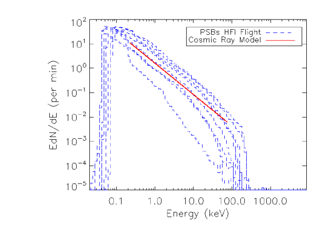
Figure 7: Energy spectrum of some typical HFI in-flight bolometers (blue dashed lines) together with the predictions (red line).

By integrating over the solid angle, the surface and the integration time, we obtain an analytical equation for the number of events per unit of absorbed energy as:

$$\frac{\Delta N}{\Delta E_{abs}}=\frac{4\pi N_{0}\Delta tE_{p^{+}o}}{(2\gamma+\beta-1)\cdot E_{O}^{\frac{\beta-1}{\gamma}}}\cdot E_{die}^{-\frac{\gamma+1-\beta}{\gamma}},$$ (1)

where $N_{0}$ is the amplitude of the spectrum of incoming protons or alpha particles at L2, $\Delta t$ the integration time, $E_{p^{+}o}$ the reference proton energy, $\gamma$ and $\beta$ are the power-law indexes of the fit between the stopping power function and the energy distribution of the proton at L2 respectively, $E_{O}=\rho_{sil}\cdot d\cdot SP(E_{p^{+}o})$ is the reference absorbed energy for an orthogonal impact, $\rho_{sil}$ the density of the silicon, $d$ the thickness of the silicon die, $SP(E_{p^{+}o})$ the stopping power function calculated at a reference proton energy, and $E_{die}$ is the energy absorbed by the silicon die.

The predictions of this model for protons are shown in Figure 7, together with the energy spectrum measured in bolometer data. The power-law index fits well with the flight data and the model is able to cover almost all the range of energies. We conclude that in terms of rate and energy distribution the thermal coupling between the silicon die and the NTD thermometer likely explains the long glitches seen in HFI in-flight data. The model shows the cut off of the long glitches distribution of the low signal is close to the noise level which is a critical point in terms of cosmological HFI goals.

5.3 Slow glitches origin

Slow glitches are the rarest events we see in terms of individual glitches on the HFI in-flight bolometers. They affect only the polarized PSBa bolometers with a rate of a few per hour in flight. The energy distribution of the slow glitches shows the same power-law index of the corresponding long glitches energy distribution (see Fig.5). In addition, the slow glitches share the template of the long glitches, but without the shortest time constant. These slow glitches were not reproduced during any of the HFI ground-based tests, both pre-launch with the HFI focal plane unit (FPU), and post-launch with flight-spare hardware. In light of this fact, we are limited to putting forward an hypothesis on the slow glitches origin that is consistent with our current results, but is without experimental confirmation. The presence of the feed-through connecting the PSBa bolometer to its corresponding silicon die is the only difference between the PSBa bolometers and the other types of bolometers in HFI, i.e., both PSBb and SWB bolometers. The PSBa feed-through elements have a strong thermal coupling with the system silicon die and gold pad. A proton hitting a PSBa feed-through, therefore, can heat the corresponding silicon die to produce a heat diffusion from the silicon die to the NTD thermometer. This heating would be without the corresponding ballistic heat conduction associated with a silicon die/CR glitch event, and therefore no fast time constant would be observed. The differences in the effective surface area of the feed-throughs with respect to the corresponding silicon dies, of a factor of about 100, may explain the differences in the rate between the long glitches and the slow glitches.

6 Conclusion

Understanding the origin and the features of glitches is of primary importance to manage systematic errors associated to the cosmic rays⁵. In addition to direct impact between the cosmic particles and the sensitive parts of the bolometers, it appeared that hits on the silicon die are also detectable and are a few tens time more numerous than the expected component. Moreover, the solar activity was extremely low at the beginning of the mission, and so the flux of cosmic ray was unusually high.

The effort done by the collaboration allowed to obtain data of excellent quality to make the maps but 20 to 12% of the samples are discarded due to glitch contamination¹. To minimise the cosmic flux, for a balloon or a space experiment using low temperature devices, it is preferable to try to avoid deep solar minimum, in particular the lowest one which occurs with a period of 100 years. But then, the experiment can suffer from solar flares so a trade-off has to be done. The crucial point, which is more manageable than the solar meteorology, would be the improvement of the isolation between the die and the sensitive part of the bolometer by an order of magnitude. Then the rate of glitches coming from the bolometer and the silicon die will be comparable, even during a period of small solar activity. The implications of this work for future satellite come from the need to improve by at least one order of magnitude the Noise Equivalent Power of new space experiments (from $10^{-17}$ $W$ / $\sqrt{Hz}$ to $10^{-19}$ $W$ / $\sqrt{Hz}$). This can be reached by increasing the focal plane coverage, using thousands of Background Limited Instrument Performance (BLIP) contiguous pixels. Each pixel of these arrays must be micro-machined starting from a common substrate. For these raisons, the influence of cosmic rays for future space detectors, must be taken into account from the very first phases of the design in parallel with all the other characteristics like NEP and time response. In particular, beam testing should be planned to study irradiation on whole array of detectors (pixels, substrate and housing).

References

- 1 Planck Collaboration submitted to A&A arXiv:1303.5062v1 (2013).
- 2 Planck Collaboration A&A 536 A2 (2011).
- 3 Planck HFI Core Team A&A 536 A4 (2011).
- 4 Planck Collaboration results X submitted to A&A, arXiv:1303.5071 (2013).
- 5 Masi, S and Battistelli, E.S. and de Bernardis, P. and Lamagna, L. and Nati, F. and Nati, L. and Natoli, P. and Polenta, G. and Schillaci, A&A 519 id.A24 9 pp. (2010)
- 6 Adriani, O. and Barbarino, G. C. and Bazilevskaya, G. A. and Bellotti, R. and Boezio, M. and Bogomolov, E. A. and Bonechi, L. and Bongi, M. and Bonvicini, V. and Borisov, S. and Bottai, S. and Bruno, A. and Cafagna, F. and Campana, D. and Carbone, R. and Carlson, P. and Casolino, M. and Castellini, G. and Consiglio, L. and De Pascale, M. P. and De Santis, C. and De Simone, N. and Di Felice, V. and Galper, A. M. and Gillard, W. and Grishantseva, L. and Jerse, G. and Karelin, A. V. and Koldashov, S. V. and Krutkov, S. Y. and Kvashnin, A. N. and Leonov, A. and Malakhov, V. and Malvezzi, V. and Marcelli, L. and Mayorov, A. G. and Menn, W. and Mikhailov, V. V. and Mocchiutti, E. and Monaco, A. and Mori, N. and Nikonov, N. and Osteria, G. and Palma, F. and Papini, P. and Pearce, M. and Picozza, P. and Pizzolotto, C. and Ricci, M. and Ricciarini, S. B. and Rossetto, L. and Sarkar, R. and Simon, M. and Sparvoli, R. and Spillantini, P. and Stozhkov, Y. I. and Vacchi, A. and Vannuccini, E. and Vasilyev, G. and Voronov, S. A. and Yurkin, Y. T. and Wu, J. and Zampa, G. and Zampa, N. and Zverev, V. G. Science 332 69 (2011)
- 7 Mewaldt, R. A. and Davis, A. J. and Lave, K. A. and Leske, R. A. and Stone, E. C. and Wiedenbeck, M. E. and Binns, W. R. and Christian, E. R. and Cummings, A. C. and de Nolfo, G. A. and Israel, M. H. and Labrador, A. W. and von Rosenvinge, T. T. ApJ 723 L1-L6 (2010).
- 8 Leske R. A. and Cummings A. C. and Mewaldt R. A. and Stone, E. C. Space Sci. Rev 126 126 (2011).
- 9 Mohammadzadeh, A. and Evans, H. and Nieminen, P. and Daly, E. and Vuilleumier, P. and Buhler, P. and Eggel, C. and Hajdas, W. and Schlumpf, N. and Zehnder, A. and Schneider, J. and Fear, R. Nuclear Science, IEEE 50 2272-2277 (2003).
- 10 Holmes, W. A. and Bock, J. J. and Crill, B. P. and Koch, T. C. and Jones, W. C. and Lange, A. E. and Paine, C. G. Appl. Opt. 47 5996 (2008).
- 11 Caserta, A. and de Bernardis, P. and Masi, S. and Mattioli M., Nuclear Instruments and Methods in Physics Research A 294 Issue 1 328-334 (1990).