Systemic risk in dynamical networks with stochastic failure criterion

Abstract

Complex non-linear interactions between banks and assets we model by two time-dependent Erdős Renyi network models where each node, representing bank, can invest either to a single asset (model I) or multiple assets (model II). We use dynamical network approach to evaluate the collective financial failure—systemic risk—quantified by the fraction of active nodes. The systemic risk can be calculated over any future time period, divided on sub-periods, where within each sub-period banks may contiguously fail due to links to either (i) assets or (ii) other banks, controlled by two parameters, probability of internal failure $p$ and threshold $T_{h}$ (“solvency” parameter). The systemic risk non-linearly increases with $p$ and decreases with average network degree faster when all assets are equally distributed across banks than if assets are randomly distributed. The more inactive banks each bank can sustain (smaller $T_{h}$), the smaller the systemic risk—for some $T_{h}$ values in I we report a discontinuity in systemic risk. When contiguous spreading becomes stochastic (ii) controlled by probability $p_{2}$—a condition for the bank to be solvent (active) is stochastic—the systemic risk decreases with decreasing $p_{2}$. We analyse asset allocation for the U.S. banks.

I Introduction

Phase transitions, critical points, hystereses and regime shifts are basic blocks describing the phase flipping of a complex dynamical system between two or more phases May08 . One of the systems having these properties is the financial system that can be considered as a system flipping over time between mainly stable phase, representing good years, and mainly instable phase, representing bad years. In the financial system, the transition from mainly stable to mainly instable phase can be triggered either by an outside sudden event such as a war or by a bankruptcy of a huge bank where the financial contagion can spread due to interlinks between financial units. The nature of this contagion spreading implies that a network approach can be the best suitable framework to describe not only financial contagion but also financial crises JPE1983 ; JPE2000 ; GaleAER ; GolobAER ; Gai10 ; Beale11 ; Guido13 ; May08 ; May10 ; May12 ; Lorenz ; Acemoglu ; Bisias ; Schweitzer ; Soramaki . In networks, just like in financial systems, the existing nodes can be rewired, and new links and nodes can be added and removed as time elapses and node’s properties can change over time Albert00 ; Vespignani01 ; Garlaschelli03 ; ParshaniPNAS ; Cohen00 ; NC ; Holme12 .

In seminal work on network approach in finance, Allen and Gale JPE2000 argued that a more interelated network may help that the losses of a disstressed bank are shared among more creditors reducing the impact of negative shocks to each individual bank. Using a network model of epidemics where nework is characterized by its degree distribution, Gai and Kapadia Gai10 showed that a large rare shock may have different consequences depending on where it hits in the network and what is the average degree of the network. In contrast, beyond a certain point, such interconnections may serve as a mechanism for propagation of large shocks leading to a more fragile financial system. Beale et al Beale11 focused on vulnerability of financial system, precisely on the friction of interest between individual banks and entire economy. The authors investigated the relationship between the risk taken by individual banks and the systemic risk associate with multiple bank failures. Arinaminpathy, Kapadia and May May12 reported how imposing tougher capital requirements on larger banks than smaller ones can increase the resilience of the financial system. Elliot, Golob, and Jackson GolobAER reported how integration (each organization becoming more dependent on its counterparties) and diversifications (each organization interacting with a larger number of counterparties) have different effects on cascading failure. Acemoglu, Ozdaglar, and A. Tahbaz-Salehi  Acemoglu reported that financial contagion exhibits a phase transition as interbank connectivity increases. If shocks are smaller than some threshold, more linked network enhance the stability of the system. However, for shocks larger than the threshold, more linked network facilitate financial contagion.

II Results

The global financial crisis has urged the need for analysing systemic risk representing the collective financial failure Lorenz ; GolobAER ; Gai10 ; GaleAER ; May08 ; Beale11 ; Guido13 ; May10 ; May12 . The majority of literature on systemic risk is focused on how the financial system responds to the failure of a single bank. However, in real finance many banks can fail inherently either simultaneusly or at different times. Here, in order to estimate the collective financial failure when multiple initial failures are possible occuring presumably at various moments, we model complex non-linear interaction between banks and firms by two variants of the dynamical Erdős Renyi network proposed in Ref. Antonio14 , where nodes (banks) contiguously fail due to links to both (i) assets and (ii) other banks, and (iii) possibly recover. In Ref. Antonio14 , the collective phenomena reported in a financial system—phase transitions, critical points, hystereses and phase flipping—have been described by the dynamical network approach. It has been explained how the network, due to (ii) stochastic contiguous spread among the nodes, may lead to the spontaneous emergence of macroscopic phase-flipping phenomena. In our dynamical network approach, bank $i$ can internally fail at any moment $t_{i}$, and once it fails, the contagion spreads at $t_{i+1}$ on $i$’s nearest neighbours, at $t_{i+2}$ on $i$’s second neighbours, and so on. This approach allows us to calculate the systemic risk at different future time horizons. The probability parameter, controlling the macroscopic phase-flipping phenomena Antonio14 , determines also that the condition for a bank to be solvent (active) is not deterministic Gai10 , but stochastic.

Qualitatively it is known that more links between banks may reduce the risk of contagion  JPE2000 . Recently a model of contagion in financial networks has been proposed Gai10 where each bank $i$ has interbank assets $A^{B}_{i}$, interbank liabilities $L^{B}_{i}$, deposits $D_{i}$ and illiquid assets $A^{M}_{i}$, and the condition for the bank to be solvent (active) is $(1-\phi)A^{B}_{i}+A^{M}_{i}-L^{B}_{i}-D_{i}>0$—a bank’s assets must ecxeed its liabilities—where $\phi$ is the fraction of inactive neighbouring banks. To account for possibility that many banks can fail at any moment—not only at initial moment—and to account for possibility to estimating bank risk for different future time horizons, highly volatile financial networks in this work we model by a variant of the dynamical Erdős Renyi network Antonio14 . We define I in the following:

• nodes represent banks, and bank $i$ at time $t$ fails if $(1-\phi_{t,i})A^{B}_{i}+A^{M}_{t,i}-L^{B}_{i}-D_{t,i}\leq 0$. The previous time-dependent condition can be accomplished if (i) bank $i$ internally fails randomly and independently of other nodes with probability of failure $p$ (see Methods)—for each bank $i$, with probability $p$, $A^{M}_{t,i}-D_{t,i}$ becomes negative and $i$ fails, regardless of interbank assets.

• Besides internally, in I bank $i$ can also fail with probability $p_{2}$ if it has less than $100T_{h}\%$ active neighbours (where $i$ sets its interbank assets) Antonio14 ; Pod13 . If not stated differently, here we assume that $p_{2}=1$, implying that if bank $i$ has $<100T_{h}\%$ active banks, it deterministically fails. The parameter $T_{h}$ measures the robustness of bank network—the smaller the parameter $T_{h}$, the more robust the bank network. Note that $T_{h}$ can be related with the criterion for bank failures of Ref. Gai10 . To this end, let’s assume that for each bank there is a linear dependence between asset $A^{B}_{i}$ and network degree $k$—e.g. $A^{B}_{i}=k_{i}$. Since the number of incoming and outgoing links is equal, it holds $A^{B}_{i}=L^{B}_{i}$. Expressing $A^{M}_{i}$ and $D_{i}$ at $t=0$ as proportional to $k_{i}(A^{B}_{i})$, when $i$ active, say $A^{M}_{t=0,i}=0.6k_{i}$ and $D_{t=0,i}=0.3k_{i}$, then bank $i$ is inactive if $\phi_{t,i}\geq 0.3\equiv\phi_{h}$ (if at least $30\%$ neighbouring banks are inactive, or alternatively, if less than $70\%$ neighbouring banks are active). Thus,

  $$1-T_{h}=\phi_{h}.$$ (1)

• In I after a time period $\tau$, the nodes recover from internal failure (see Methods). In finance, this $\tau$ is comparable with an average time a firm spends in financial distress that is approximately two years for U.S. firms Eberhart .

Figure 1: Dependence of network systemic risk of banks, $1-f_{n}$ (fraction of failed banks), on network parameters, individual probability of bank failure $p$, threshold $T_{h}$, and network degree, $\langle k\rangle$. We use ER dynamical network of Ref. Antonio14 , where banks fail independently of each other. (a)-(b) $1-f_{n}$ increases with $p$ for varying $T_{h}$ and $\langle k\rangle$. (c) $1-f_{n}$ non-continuously increases with $T_{h}$. (d) $1-f_{n}$ decreases with $\langle k\rangle$ for large values of $\langle k\rangle$.

To calculate how the systemic risk—among many different definitions Bisias , here defined as the fraction of failed banks—depends on the model parameters, first we present an analytical result that holds for mean-field approximation, which is generally valid for a network with large number of nodes and degrees. If internal ($X$) and external ($Y$) failures are independent, Ref. Antonio14 calculated the probability, $a=a(p,p_{2},T_{h})\equiv P(X\cup Y)$, that a randomly chosen bank node $i$ is inactive $a=p+p_{2}(1-p)\Sigma_{k}P(k)E(k,m,a)$. This probability is equal to the fraction of inactive bank nodes, $a=1-\langle f_{n}\rangle$. Here $P(k)$ is the degree distribution of the inter-bank links, and parameters $p$, $T_{h}$, and $p_{2}$ are explained in I. $E(k,m,a)\equiv\Sigma_{j=0}^{m}a^{k-j}(1-a)^{j}{k\choose k-j}$ is the probability that node $i$’s neighbourhood is critically damaged Antonio14 , where $k$ is the number of links of node $i$, and $m\equiv T_{h}k$. For $m=1$ we provide an analytical form of $a=1-\langle f_{n}\rangle$ when $P(k)$ is the Poisson distribution $P(k)=(\langle k\rangle)^{k}e^{-\langle k\rangle}/k!$—we obtain $a=p+p_{2}(1-p)(1+\langle k\rangle-a\langle k\rangle)e^{\langle k\rangle(a-1)}$.

Application of analytical results based on mean field approximation in finance—where generally there are either small or moderately large number of banks—is highly limited since for these cases the mean field holds only approximately Antonio14 . For these cases, in practice, numerical approach helps us estimate how the systemic risk quantitatively depends on each model parameters and finally enable us to, using regression, estimate what the systemic risk is for a given set of empirically estimated parameters.

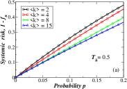
For dynamical Erdős Renyi network I with 1,000 banks, in numerical simulations each of 10,000 runs is used to estimate e.g. the systemic risk a year ahead expressed as the fraction of failed banks, $1-f_{n}$. Each run we accomplish in two time steps and each bank can internally fail in both time steps with no recovery $(\tau>2)$. By fixing parameters $\langle k\rangle$ and $T_{h}$, in Fig. (1)(a)-(b) we find that the bank systemic risk, $1-f_{n}$, increases non-linearly with individual bank failure $p$. In Fig. (1)(a) the systemic risk decreases with the average degree $\langle k\rangle$. Thus, the larger the number of links between banks, the smaller the systemic risk. This result is in agreement with Ref. JPE1983 where it was shown that networks with more links are less vulnerable than networks with a few links, since the fraction of the losses in one bank is transferred to more banks through interbank links. Note that our choice $\langle k\rangle=15$ is due to Ref.Soramaki reporting that the average bank in the U.S. is linked to $15$ others, however most banks has only few connections while a small number of huge banks have thousands.

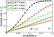
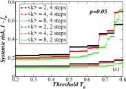
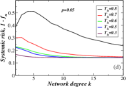
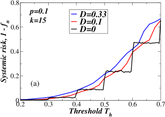
In Fig. (1)(b) we report that the more failed neighbouring banks any bank can sustain (the smaller $T_{h}$), the smaller the systemic risk. In economics, the existence of threshold assumes that when an organization’s value (say asset minus debt) hits a failure threshold, the organization discontinuosly can lose part of its value GolobAER . Due to interdependencies among nodes, individual failues may trigger collective cascade of failures. To this end, with increasing $T_{h}$ the systemic risk in Fig. (1)(c) exhibits a non-linear discontinuity where $1-f_{n}$ suddenly jumps at some critical points in $T_{h}$ such as $1/2,2/3,...$, since link values are integer numbers. Note that Ref. Antonio14 reported a discontinuity in the fraction of active nodes, $f_{n}$, when increasing (decreasing) $p$ and $p_{2}$, together with the hysteresis property that is the characteristic feature of a first-order phase transition Antonio14 ; Pod13 . As stated in Introduction, recently Ref. Acemoglu reported phase transition as interbank links increases. Next, Fig. (1)(d) confirms again that the systemic risk in dynamical network approach decreases with $\langle k\rangle$.

For many parameter sets ($\langle k\rangle$, $T_{h}$, $p$, $1-f_{n}$) obtained from each two-period runs (where $\tau>2$, thus no recovery), we perform linear regression analysis $1-f_{n}=\alpha+\alpha_{p}p+\alpha_{T}T_{h}+\alpha_{k}k$, and obtain $\alpha=-0.016\pm$ 0.001, $\alpha_{p}=2.20\pm 0.03$, $\alpha_{T}=0.067\pm 0.005$, and $\alpha_{k}=-0.0017\pm 0.0002$. The systemic risk significantly increases with $p$ and $T_{h}$, while decreases with degree $\langle k\rangle$. Note that these values we obtained using $p\in(0,0.1)$, $T_{h}\in(0.2,0.8)$, and $\langle k\rangle\in(2,20)$.

Dynamical network approach reveals one more forecasting benefit. It provides us with forecasting power for generally any future time horizon. For the dynamical Erdős Renyi network I in Fig. (1)(b) we show the expected systemic risk where each of 10,000 runs is composed of four steps. If each time step represents, say semi-year period, than two-step systemic risk represents our estimation for systemic risk a year ahead, while four-step systemic risk represents our estimation for systemic risk two years ahead. As expected for the case with no recovery, four-step systemic risk is larger than two-step systemic risk. Similar result we obtain in Fig. (1)(c) where for $\langle k\rangle=8$ we show that four-step systemic risk is substantially larger than two-step systemic risk. Note that these results we obtain under assumption that banks and assets, once failed, do not recover. Clearly, in more reliable dynamical network approach one should also define how assets and banks recover over time after, for example, the government intervenes in the market.

Figure 2: For fixed $p$ and (b) $T_{h}$, with decreasing parameter $p_{2}$ (from 1 to 0), the systemic risk decreases. We set $\langle k\rangle=8$ and $T_{h}=0.5$ in (a).

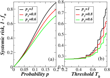
Figure (2) shows that for fixed $p$ and $T_{h}$, the systemic risk decreases with decreasing parameter $p_{2}$ (shown from 1 to 0.6), that is a reasonable result since $p_{2}=1$ implies that a bank deteministicly fails when a criterion for insolvency $(1-\phi_{t,i})A^{B}_{i}+A^{M}_{t,i}-L^{B}_{i}-D_{t,i}\leq 0$ is fulfilled, while when $p_{2}\neq 1$, there is some chance that the bank will not fail. This unpredictability is something that really occurs in real market, since bankruptcy is not deterministic event. However, stochasticity is not important only at microscopic firm (bank) level. Ref. Antonio14 reported that introduction of stochasticity leads to emergence of macroscopic phase-flipping between “active” and “inactive” macroscopic phases that are demonstrated in Ref. Pod13 for “expansion” and “recession” phases in economy.

In the previous network I it was assumed that each bank can independently internally fail. Next we propose another network model II (see Methods), where each bank can put its money not only in other banks, as in I, but also in different illiquid asset classes ${\cal A}_{t,i}^{M}$. Since different banks can invest their money in equal assets ${\cal A}_{t,i}^{M}$, banks’ failures are now not independent. In contrast to banks’ failures, ${\cal A}_{t,i}^{M}$’s failures are assumed to be independent to each other. For simplicity, we define that firms can affect banks, but not vice versa as in Gai10 ; May12 ; Caccioli .

Figure 3: (a) Systemic risk for bank network increases with time spent in failure $\tau$. (b) Systemic risk for different time scales. With increasing the time horizon, the systemic risk also increases.

Figure 4: Dependence between (a) firms and (b) banks arises from the dynamical network model where firm failures may affect all banks having investments in those failed firms. We set $\tau=50$, $p=0.004$, $p_{2}=0.8$, $\langle k\rangle=4$, and $T_{h}=0.5$. Periods characterized by the largest spikes in the fraction of failed firms coincide with the spikes in the fraction of failed banks. Both fractions of (a) failed assets and (b) failed banks are increased where the fraction of failed banks are characterized by three states, one with virtually no failed nodes, and two states with different fractions of failed nodes.

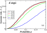
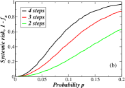
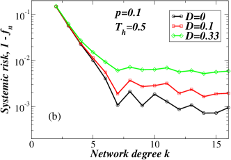
In the following simulations we include recovery process. In II there are four time steps in our analysis, but this time we change the time period needed for recovery, $\tau$. For (i)-(iii) ER dynamical network with finite number of banks, $N_{b}=1000$, and assets, $N_{f}=10$, our numerical simulations in Fig. (3)(a) confirm that the systemic risk calculated for bank network—defined by the fraction of banks in failure—increases with the individual probability of asset failure $p$, chosen to be equal for each asset. We assume as in Ref. May12 that both large and small banks hold the same number of asset classes, $10$. We perform $10^{5}$ simulations in order to estimate expected systemic risk where each simulation itself we perform in four steps with $\tau$ meaning that once a bank or an asset is failed, it stays failed for the entire period $\tau$. Figures (3) reveals that this dynamical network II exhibits highly non-linear properties. By first fixing parameter $T_{h}$, in Fig. (3)(a) for II we find that the systemic risk for bank network increases with $\tau$. The longer time a bank stays in failure, the larger the systemic risk. In Fig. (3)(b) we show how dynamical approach enables us to estimate the systemic risk for different time horizons. As expected, with increasing the time horizon, the systemic risk also increases.

Figure 5: Smile-form in probability of individual bank failure with two assets with allocations $W_{1}$ and $W_{2}$. The smallest risk occurs as expected for $W_{1}=W_{2}=0.5$. We use $\tau=2.5$.

Figure 6: Dependence of diversification of assets on systemic risk within dynamical network approach. (a) Systemic risk increases with $T_{h}$ for varying $D$ value. $D$ quantifies the level of asset allocation. With increasing randomness in asset allocation, where $D$ increases from zero to $1/3$, the systemic risk increases. We use that $p_{2}=1$ and $T_{h}=T^{\prime}_{h}$ (see Methods). (b) Systemic risk decreases with average network degree $\langle k\rangle$.

In order to analyse how banks and assets interact with each other over time, we evolve simultaneously both banks and assets. In Fig. (4) we show how the fractions of failed $(N_{f}=10)$ assets and $(N_{f}=1000)$ banks change over time for a given set of parameters, where recovery exists. Note how the periods when many assets are dysfunctional coincide with the periods when many banks are dysfunctional, in agreement with our model assumption that asset failures may affect bank failures in all banks having investments in the failed assets.

Our network model II is partially motivated by Beale et al Beale11 . As known in finance, each bank can reduce its probability of failure by diversifying its risk Markowitz . However, when many banks diversify their risks in similar way, the probability of multiple failure increases Beale11 . For the case with $N$ banks and $M$ assets, Beale11 defined the total loss incurred by bank $i$ after one period $Y_{i}=\sum W_{ij}V_{j}$, where the failure occurs if its total losses exceed a given threshold $\gamma_{i}$, i.e. $Y_{i}>\gamma_{i}$. Here, $W_{ij}$ denotes bank $i^{\prime}$s allocation in asset $j$, $V_{j}$ is the loss in asset $j$’s value taken from a student $t$ distribution, and $\gamma_{i}$ is a threshold.

In model II we use not $t$ distribution as in Ref. Beale11 , but a simpler Laplace distribution and derive a probability of bank failure with two assets with allocations $W_{1}$ and $W_{2}$:

$$P = \frac{\exp(-\frac{\gamma}{W_{2}\tau})}{4(1+\frac{W_{1}}{W_{2}})}+\frac{\exp(-\frac{\gamma}{W_{2}\tau})}{4(1-\frac{W_{1}}{W_{2}})}(1-\exp(-\frac{(1-\frac{W_{1}}{W_{2}})\gamma}{W_{1}\tau}))$$

$$+ \frac{\exp(-\frac{\gamma}{W_{1}\tau})}{2}+\frac{\exp(\frac{\gamma}{W_{2}\tau})}{4(1+\frac{W_{1}}{W_{2}})}\exp(-\frac{(1+\frac{W_{1}}{W_{2}})\gamma}{W_{1}\tau}).$$

This expression, numerically tested in Fig. (5), gives the same smile-form for the probability of bank failure as numerically found in Ref. Beale11 . Next we analyse how diversification of asset allocations affects systemic risk within the dynamical network approach. To this end, Ref. Beale11 proposed a measure to estimate the level of asset allocation

$$D=\frac{1}{2N(N-1)}\sum_{i=1}^{N}\sum_{j=1}^{N}\sum_{l=1}^{M}|W_{i,l}-W_{j,l}|$$ (2)

in order to quantify the average of the distances between each pair of banks’ asset allocations, where $D=0$ if each bank invests equally in each asset, thus if $W_{i,j}=1/M$ for each $i$ and $j$. Thus, when many banks decide to invest with similar portfolios, they may increase the chance to fail simultaneously. In Fig. (6)(a) within dynamical network approach, we obtain that the lowest systemic risk occurs when all assets are equally distributed across banks, that is in agreement with the result obtained in Ref. Beale11 where banks do not affect each other, and systemic risk is defined as expected number of failures. With increasing randomness in asset allocation, where $D$ increases from zero to $1/3$, the systemic risk also increases. As a new result arising from the network approach, in Fig. (6)(b) we obtain that the systemic risk decreases with average degree $\langle k\rangle$ faster when asset allocation is more homogeneous.

To see how well the real market can withstand systemic risk, we exam the level of diversification of asset allocation for the U.S. commercial banks. Here, based on 64,289 commercial banks’ balance sheet, we analyze their loan allocations in 10 different sectors Huang13 : Loans for Construction and Land Development Loans Secured by farmland, Mortgages Secured by 1-4 Family residential properties, Loans Secured by multifamily ($>5$) residential properties, Loans Secured by nonfarm nonresidential properties, Agricultural Loans, Held-to-Maturity securities, Commercial and industrial loans, others, Available-for-sale securities, Loans to Individuals. The first five sectors are under the asset class of Real Estate which is the biggest part of the banks’ loans allocations. Hence we decompose them to smaller sub-sectors. The data are collected from 1/1/1976 - 12/31/2008 and a considerable fraction of the banks have disappeared during the period. We use Eq. (2) to calculate the average diversification of the commercial banks, and find $D=0.51$, a larger value than $D=0.33$, obtained for random diversification. It indicates that in real market, diversification of banks puts the systems at a riskier regime than random diversification.

III Discussion

Generally, the systemic risk risk may arise either because banks diversify their risks in firms in similar ways Beale11 or because banks are linked within a bank network and thus failures can spread contiguouslyJPE1983 ; JPE2000 ; GaleAER . For the dynamical (time-dependent) network Antonio14 where nodes (i) inherently fail, (ii) contiguously fail, and (iii) recover, when applied to finance, the stochastic contiguous spreading controlled by parameter $p_{2}$ corresponds to a stochastic condition for the bank to be solvent (active in network terms). We demonstrated how the systemic risk in the dynamical (time-dependent) network depends on dynamical network parameters: probability of individual asset failure $p$, bank vulnerability parameter $T_{h}$, and average network degree $\langle k\rangle$. We found that the more inactive banks each bank can sustain ($T_{h}$ closer to zero), the smaller the systemic risk. For fixed $p$ and $T_{h}$, the systemic risk decreases with decreasing parameter $p_{2}$ (increasing stochasticity). This result is reasonable because when a criterion for a bank’s insolvency is met and $p_{2}\neq 1$, there is some chance that the bank will not fail. In practice, the parameter $T_{h}$ can be controlled by the government or banks. Our analysis showed that having $T_{h}\lesssim 0.4$ enables the system to function with low risk for a large set of parameters $p$ and $\langle k\rangle$. We demonstrated how the dynamical network approach enables us to estimate systemic risk for different future time scales. We also showed how the systemic risk depends on the level of asset allocation. The dynamical network approach enables to estimate systemic risk in a wide range of financial systems from pension, mutual, and hedge funds to banking system.

IV Methods

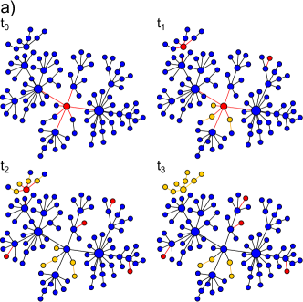
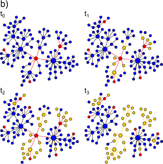
We defined the network model I in Results and here we explaine the model graphically. In Fig. (7)(a) we choose $\tau=2$, $T_{h}=0.5$, and $p_{2}=1$, where the last choice for $p_{2}$ implies that the solvency criterion is deterministic. Due to dynamical time-dependent network approach, in Fig. (7)(a) we see how different nodes become internally failed at different times. Due to the choice for the value of $T_{h}$, the financial contigion is not spread to the nearest hubs (note that a bank deterministically fails if it has less than $100T_{h}\%$ active neighbours). In Fig. (7)(b) we choose $\tau=3$ and $p_{2}=0.8$ where the last choice for $p_{2}$ implies that the solvency criterion is now stochastic. Now we choose the larger $T_{h}$ than in (a), $T_{h}=0.8$, meaning that each bank is more dependent to failures of its neigbours than in (a). Now we see in Fig. (7)(b) how the financial spreading is more devastating then in case (a). Note that, due to stochasticity in the solvency criterion, some nodes which would be externally inactive due to deterministic criterion in (a) are now in (b) externally active.

We define the network model II in the following:

• At each time $t$, each of $N_{f}$ assets ${\cal A}_{t,i}^{M}$ can independently fail where the probability $p$ of failure for each ${\cal A}_{t,i}^{M}$ is equal and is taken from a Laplace (double) exponential distribution, ${\cal L}(x)$. We define that asset ${\cal A}_{t,i}^{M}$ fails if the Laplace variable $x$ is smaller than some threshold, $P_{h}$—thus, $p=\int_{-\infty}^{P_{h}}dx{\cal L}(x)$. For simplicity, assets do not influence each other. Once asset ${\cal A}_{t,i}^{M}$ fails, it stays in failure with no possibility for recovery.

• Each of the $N_{b}$ nodes representing banks, for simplicity reason, has the same asset and liability values as in example in I—so, bank $j$ at time $t=0$ has $A^{B}_{j}=k_{j}$, $A^{M}_{t=0,j}=0.6k_{j}$ and $D_{j}=0.3k_{j}$ (here $D_{j}$ does not change in time), but the results are robust to different allocations. However, this time the total illiquid asset $A^{M}_{t=0,j}$ is allocated across $N_{f}$ assets. Precisely, at initial time $t=0$ every bank $j$ determines how much money $W_{j,i}$ to invest in asset ${\cal A}_{i}^{M}$, where $W_{j,i}$ is taken randomly from the homogeneous distribution after proper normalization, where clearly for each $j$, $\sum_{i=1}^{N_{f}}W_{j,i}=A^{M}_{t=0,j}$, where the sum runs over all assets. Since at each moment assets can be either active or inactive (failed), at each $t$, bank $j$ has the total illiquid asset equal to $A^{M}_{t,j}=\sum_{i=1}^{N_{f}}W_{j,i}\delta_{i}(t)\leq A^{M}_{0,j}$, where $\delta_{i}(t)$ at time $t$ can be either one or zero depending whether asset ${\cal A}_{i}^{M}$ is active or inactive. The more robust the bank, the larger the fraction of failed assets the bank can sustain without getting failed. Here we define that bank $j$’s node becomes internally contiguously failed due to links to assets if $A_{t,j}^{M}\leq T^{\prime}_{h}A_{t=0,j}^{M}$, where $T^{\prime}_{h}$ is the given threshold. Bank $j$ internally fails if $A^{M}_{t,j}-D_{j}<0$ and from our choice for $A^{M}_{t=0,j}=0.6k_{j}$ and $D_{j}=0.3k_{j}$ the failure occurs when $T^{\prime}_{h}=0.5$. We define bank node $j$’s internal failure state by spin $|s_{j}\rangle$.

• In our financial network, a bank can fail either due to illiquid asset’ failures or due to banks’ failures. Here the concept of a network is used to model interbank lending and to study the phenomena of financial stability and contagion JPE1983 ; JPE2000 ; GaleAER . At initial time, banks create links among themselves through exchanging deposits to insure themselves against contagion JPE2000 . To this end, external failure state of bank node $j$ denoted by spin $|S_{j}\rangle$ is $|0\rangle$ (during a time $\tau^{\prime}=1$) with probability $p_{2}$ if less than $100\cdot T_{h}~{}\%$ of $j$’s neighbouring links are active Antonio14 . Bank node $j$—described by the two-spin state $|s_{i},S_{i}\rangle$—is active only if both spins are 1, i.e, $|s_{i},S_{i}\rangle=|1,1\rangle$. Links between banks are bidirectional. Having two spins, representing a financial health of a bank, assumes that a bank fails either if it made bad investments in firms or in other banks—alternatively if it is surrounded by bad neighbours. We assume $A^{M}_{0,j}=0.6k_{j}$, $D_{j}=0.3k_{j}$ (the same choices as in I), and $A^{B}_{j}=k_{j}$. For this choice of allocations, if we assume that all illiquid assets where $j$ invested are active, we obtain $T_{h}=0.7$ $(\phi_{h}=0.3)$ (see Eq. (1)). Suppose that at time $t$ some illiquid assets ($20\%$) are inactive and $A^{M}_{t,j}=\sum_{i=1}^{N_{f}}W_{j,i}\delta_{i}(t)=0.8A^{M}_{0,j}=0.48k_{j}$. From insolvency criterion $(1-\phi_{t,i})A^{B}_{i}+A^{M}_{t,i}-L^{B}_{i}-D_{t,i}\leq 0$ we obtain $\phi_{t,i}\geq 0.18\equiv\phi_{h}$. Hence, the larger the fraction of inactive illiquid assets, the smaller the fraction of neighbouring banks required to cause the external failure.

Figure 7: Contiguous spread in model I. (a) Deterministic solvency criterion ($p_{2}=1$). For steps $t=0,1,2$, and $3$ shown is a network for $\tau=2$. Active nodes are blue, internally inactive nodes are red and externally inactive nodes are denoted by orange. Nodes can become internally inactive at any moment where congigion is spread each step towards the nearest neighbours. (b) Stochastic solvency criterion $p_{2}\neq 1$). For steps $t=0,1,2$, and $3$ shown is a network for $\tau=3$ and $p_{2}=0.8$.

References

- (1) R. M. May, S. A. Levin, and G. Sugihara, Nature 451, 893 (2008).
- (2) D. W. Diamond and P. H. Dybvig, Journal of Political Economy 91, 401 (1983).
- (3) F. Allen and D. Gale, Journal of Political Economy 108, 1 (2000).
- (4) D. M. Gale and S. Kariv, American Economic Review 97, 99 (2007).
- (5) K. Soramaki et al, Physica A 379, 317 (2007).
- (6) F. Schweitzer et al, Science 325, 422 (2009).
- (7) J. Lorenz, S. Battiston, and F. Schweitzer, Eur. Phys. Journal B 71, 441 (2009).
- (8) R. M. May and N. Arinaminpathy, J. R. Soc. Interface 7, 823 (2010).
- (9) P. Gai and S. Kapadia, Proceedings of the Royal Society of London A 466, 2401 (2010).
- (10) N. Beale et al, Proc. Natl. Acad. Sci. USA 108, 12647 (2011).
- (11) N. Arinaminpathy, S. Kapadia, and R. M. May, Proc. Natl. Acad. Sci. USA 109, 18338 (2012).
- (12) D. Delpini et al, Sci. Rep. 3, 1626 (2013).
- (13) D. Acemoglu, A. Ozdaglar, and A. Tahbaz-Salehi (2012), http://ssrn.com/abstract=2207439.
- (14) D. Bisias, M. D. Flood, A. W. Lo, S. Valavanis, Annual Review of Financial Economics 4, 255 (2012).
- (15) M. Elliott, B. Golub, and M. O. Jackson, forthcoming in the American Economic Review.
- (16) R. Albert, H. Jeong, and A. -L. Barabási. Nature 406, 378 (2000).
- (17) R. Pastor-Satorras and A. Vespignani, Phys. Rev. Lett. 86, 3200 (2001).
- (18) D. Garlaschelli, G. Caldarelli, and L. Pietronero, Nature 423, 165 (2003).
- (19) R. Parshani, S. V. Buldyrev, and S. Havlin, Proc. Natl. Acad. Sci. USA 108, 1007 (2011).
- (20) R. Cohen, K. Erez, D. ben-Avraham, S. Havlin, Phys. Rev. Lett. 85, 4626 (2000).
- (21) A. Bashan et al, Nature Communications 3, 702 (2012).
- (22) P. Holme and J. Saramaki, Phys. Reports 519, 97 (2012).
- (23) A. Majdandzic et al., Nature Physics 10, 34 (2014).
- (24) B. Podobnik et al, arXiv:1401.7450 (to appear in PRE).
- (25) A. C. Eberhart, W. T. Moore, and R. L. Roenfeldt, J. Finance 45, 1457 (1990).
- (26) F. Caccioli, T. A. Catanach, and J. D. Farmer, arXiv:1109.1213.
- (27) H. Markowitz, J. Finance 7, 77 (1952).
- (28) X. Huang, I. Vodenska, S. Havlin, and H. E. Stanley, Scientific Reports 3, 1219 (2013).