March 2014
Bayesian Reconstruction of the Velocity Distribution of
Weakly Interacting Massive Particles
from Direct Dark Matter Detection Data
Chung-Lin Shan
Physics Division,
National Center for Theoretical Sciences
No. 101, Sec. 2, Kuang-Fu Road,
Hsinchu City 30013, Taiwan, R.O.C.
Department of Physics,
Hangzhou Normal University
No. 16, Xuelin Street, Xiasha Higher Education Zone,
Hangzhou 310036, Zhejiang, China
Kavli Institute for Theoretical Physics China,
Chinese Academy of Sciences
No. 55, Zhong Guan Cun East Street,
Beijing 100190, China
E-mail: clshan@phys.nthu.edu.tw
Abstract
In this paper, we extended our earlier work on the reconstruction of the (time–averaged) one–dimensional velocity distribution of Galactic Weakly Interacting Massive Particles (WIMPs) and introduce the Bayesian fitting procedure to the theoretically predicted velocity distribution functions. In this reconstruction process, the (rough) velocity distribution reconstructed by using raw data from direct Dark Matter detection experiments directly, i.e. measured recoil energies, with one or more different target materials, has been used as “reconstructed–input” information. By assuming a fitting velocity distribution function and scanning the parameter space based on the Bayesian analysis, the astronomical characteristic parameters, e.g. the Solar and Earth’s Galactic velocities, will be pinned down as the output results.
Our Monte–Carlo simulations show that this Bayesian scanning procedure could reconstruct the true (input) WIMP velocity distribution function pretty precisely with negligible systematic deviations of the reconstructed characteristic Solar and Earth’s velocities and 1 statistical uncertainties of km/s. Moreover, for the use of an improper fitting velocity distribution function, our reconstruction process could still offer useful information about the shape of the velocity distribution. In addition, by comparing these estimates to theoretical predictions, one could distinguish different (basic) functional forms of the theoretically predicted one–dimensional WIMP velocity distribution function with 2 to 4 confidence levels.
1 Introduction
Currently, direct Dark Matter detection experiments searching for Weakly Interacting Massive Particles (WIMPs) are one of the promising methods for understanding the nature of Dark Matter (DM) and identifying them among new particles produced at colliders as well as studying the (sub)structure of our Galactic halo [1, 2, 3, 4].
In our earlier work [5], we developed methods for reconstructing the (moments of the) time–averaged one–dimensional velocity distribution of halo WIMPs by using the measured recoil energies directly. This analysis requires no prior knowledge about the WIMP density near the Earth nor about their scattering cross section on nucleus, the unique required information is the mass of incident WIMPs. We therefore turned to develop the method for determining the WIMP mass model–independently by combining two experimental data sets with two different target nuclei [6]. By combining these methods and using two or three experimental data sets with different detector materials, one could reconstruct the one–dimensional velocity distribution of Galactic WIMPs directly. However, as presented in Ref. [5], with a few hundreds or even thousands recorded WIMP events, only estimates of the reconstructed velocity distribution with pretty large statistical uncertainties at a few ( 10) points could be obtained.
Therefore, in order to offer more detailed information about the Galactic WIMP velocity distribution, we introduce in this paper the Bayesian analysis into our model–independent reconstruction procedure developed in Ref. [5] to be able to determine, e.g. the position of the peak of the one–dimensional velocity distribution function and the concrete values of the characteristic Solar and Earth’s Galactic velocities.
The remainder of this paper is organized as follows. In Sec. 2, we first review the model–independent method for reconstructing the time–averaged one–dimensional velocity distribution of halo WIMPs by using data from direct DM detection experiments directly. Then we introduce the Bayesian analysis and give the basic formulae needed in the extended reconstruction process. In Sec. 3, we present numerical results of the reconstructed WIMP velocity distribution functions based on Monte–Carlo simulations for different generating and fitting velocity distributions. Different input WIMP masses as well as impure (pseudo–)data sets mixed with (artificially added) unrejected background events will also be considered. We conclude in Sec. 4. Some technical details for our analysis will be given in Appendix.
2 Formalism
In this section, we develop the formulae needed for our Bayesian reconstruction of the one–dimensional velocity distribution function of halo WIMPs by using direct Dark Matter detection data directly.
We first review the model–independent method for reconstructing the time–averaged WIMP velocity distribution by using experimental data, i.e. measured recoil energies, directly from direct detection experiments. These “reconstructed data” (with estimated statistical uncertainties) will be used as input information for the further Bayesian analysis. Then, in the second part of this section, we review the basic concept of the Bayesian analysis and give the formulae needed in our extended reconstruction procedure.
2.1 Model–independent reconstruction of one–dimensional WIMP velocity distribution
In this subsection, we review briefly the method for reconstructing the one–dimensional WIMP velocity distribution from experimental data directly. Detailed derivations and discussions can be found in Ref. [5].
2.1.1 From the recoil spectrum
The basic expression for the differential event rate for elastic WIMP–nucleus scattering is given by [1]:
| (1) |
Here is the direct detection event rate, i.e. the number of events per unit time and unit mass of detector material, is the energy deposited in the detector, is the elastic nuclear form factor, is the one–dimensional velocity distribution function of the WIMPs impinging on the detector, is the absolute value of the WIMP velocity in the laboratory frame. The constant coefficient is defined as
| (2) |
where is the WIMP density near the Earth and is the total cross section ignoring the form factor suppression. The reduced mass is defined by
| (3) |
where is the WIMP mass and that of the target nucleus. Finally, is the minimal incoming velocity of incident WIMPs that can deposit the energy in the detector:
| (4) |
with the transformation constant
| (5) |
and is the maximal WIMP velocity in the Earth’s reference frame, which is related to the escape velocity from our Galaxy at the position of the Solar system, km/s.
In our earlier work [5], it was found that, by using a time–averaged recoil spectrum and assuming that no directional information exists, the normalized one–dimensional velocity distribution function of incident WIMPs, , can be solved from Eq. (1) directly as
| (6) |
where the normalization constant is given by
| (7) |
Here the integral goes over the entire physically allowed range of recoil energies: starting at , and the upper limit of the integral has been written as . Note that, because in Eq. (6) is the normalized velocity distribution, the normalization constant here is independent of the constant coefficient defined in Eq. (2). Hence, as the most important consequence, the velocity distribution function of halo WIMPs reconstructed by Eq. (6) is independent of the local WIMP density as well as of the WIMP–nucleus cross section . However, not only the overall normalization constant given in Eq. (7), but also the shape of the velocity distribution, through the transformation in Eq. (6), depends on the WIMP mass (involved in the coefficient defined in Eq. (5)).
2.1.2 From experimental data directly
In order to use the expressions (6) and (7) for reconstructing , one needs a functional form for the recoil spectrum . In practice this requires usually a fit to experimental data. However, data fitting will re–introduce some model dependence and make the error analysis more complicated. Hence, expressions that allow to reconstruct directly from data (i.e. measured recoil energies) have also been developed [5]. We started by considering experimental data described by
| (8) |
Here the entire experimental possible energy range between the minimal and maximal cut–offs and has been divided into bins with central points and widths . In each bin, events will be recorded.
As argued in Ref. [5], the statistical uncertainty on the “slope of the recoil spectrum”, , appearing in the expression (6), scales like the bin width to the power . In addition, the wider the bin width, the more the recorded events in this bin, and thus the smaller the statistical uncertainty on the estimator of . Hence, since the recoil spectrum is expected to be approximately exponential [5], in order to approximate the spectrum in a rather wider range, instead of the conventional standard linear approximation, the following exponential ansatz for the measured recoil spectrum (before normalized by the exposure ) in the th bin has been introduced [5]:
| (9) |
Here is the standard estimator for at :
| (10) |
is the logarithmic slope of the recoil spectrum in the th bin, which can be computed numerically from the average value of the measured recoil energies in this bin:
| (11) |
where
| (12) |
Then the shifted point in the ansatz (9), at which the leading systematic error due to the ansatz is minimal [5], can be estimated by
| (13) |
Note that differs from the central point of the th bin, .
2.1.3 Windowing the data set
As mentioned above, the statistical uncertainty on the slope of the recoil spectrum around the central point , , is approximately proportional to . Thus, in order to reduce the statistical uncertainty on the velocity distribution reconstructed by Eq. (14), it seems to be better to use large bin width. However, neither the conventional linear approximation:
| (17) |
nor the exponential ansatz given in Eq. (9) can describe the real (but as yet unknown) recoil spectrum exactly. The neglected terms of higher powers of could therefore induce some uncontrolled systematic errors which increase with increasing bin width. Moreover, since the number of bins scales inversely with their size, by using larger bins we would be able to estimate only at a smaller number of velocities. Additionally, once a quite large bin width is used, it would correspondingly lead to a quite large value of the first reconstructible point of , i.e. , since the central point as well as the shifted point of the first bin would be quite large. Finally, choosing a fixed bin size, as one conventionally does, would let errors on the estimated logarithmic slopes, and hence also on the estimates of , increase quickly with increasing or . This is due to the essentially exponential form of the expected recoil spectrum, which would lead to a quickly falling number of events in equal–sized bins. By some trial–and–error analyses it was found that the errors are roughly equal in all bins if the bin widths increase linearly [5].
Therefore, it has been introduced in Ref. [5] that one can first collect experimental data in relatively small bins and then combining varying numbers of bins into overlapping “windows”. In particular, the first window would be identical with the first bin. One starts by binning the data, as in Eq. (8), where the bin widths satisfy
| (18) |
i.e.
| (19) |
Here the increment satisfies
| (20) |
being the total number of bins, and are the experimental minimal and maximal cut–off energies. Assume up to bins are collected into a window, with smaller windows at the borders of the range of .
In order to distinguish the numbers of bins and windows, hereafter Latin indices are used to label bins, and Greek indices to label windows. For , the th window simply consists of the first bins; for , the th window consists of bins ; and for , the th window consists of the last bins. This can also be described by introducing the indices and which label the first and last bins contributing to the th window, with
| (21a) |
and
| (21b) |
The total number of windows defined through Eqs. (21a) and (21b) is evidently , i.e. .
As shown above, the basic observables needed for the reconstruction of by Eq. (14) are the number of events in the th bin, , as well as the average value of the measured recoil energies in this bin, . For a “windowed” data set, one can easily calculate the number of events per window as
| (22) |
as well as the average value of the measured recoil energies
| (23) |
where is the central point of the th window. The exponential ansatz in Eq. (9) is now assumed to hold over an entire window. We can then estimate the prefactor as
| (24) |
being the width of the th window. The logarithmic slope of the recoil spectrum in the th window, , as well as the shifted point (from the central point of each “window”, ) can be calculated as in Eqs. (11) and (13) with “bin” quantities replaced by “window” quantities. Finally, note that, due to the combination of bins into overlapping windows, these quantities are all correlated (for ). The covariance matrix of the estimates of at adjacent values of is given by111 Note that Eq. (25) should in principle also include contributions involving the statistical error on the estimator for in Eq. (16). However, this error and its correlations with the errors on the and have been found to be negligible compared to the errors included in Eq. (25) [5].
| (25) | |||||
2.2 Bayesian analysis
In this subsection, we review the basic concept of the Bayesian analysis [7] (for its applications in physics, see e.g. Ref. [8], and for its recent applications in direct DM detection phenomenology, see e.g. Refs. [9, 10, 11, 12, 13, 14]) and extend this method to the use of the “reconstructed data” offered by our model–independent reconstruction process described in the previous subsection.
2.2.1 Baye’s theorem
We start with the Baye’s theorem: the probability of given that is true multiplies the probability of that is true is equal to the probability of that and happen simultaneously, which is also equal to the probability of given that is true multiplies the probability of that is true. This can simply be expressed as
| (26) |
where is called the “conditional probability” of given that is true. As long as , the above equation can be rewritten as
| (27) | |||||
where is the probability of the complement of , i.e. the probability of that is not happen.
2.2.2 Bayesian statistics
Applying the Baye’s theorem described above, one can directly have that
| (28) |
This means that, given the observed result, the probability of that a specified theory is true is proportional to the probability of the observed result in the specified theory multiplies the probability of the specified theory.
This statement can be understood as follows. If the observed result is predicted by a specified theory to be highly unlikely or even impossible/forbidden, then this observation makes the “degree of belief” of this specified theory small or even disproves this theory. In contrast, the observation of a prediction by a specified theory with a high probability will strengthen one’s belief in this theory.
2.2.3 Bayesian analysis
By extending Eq. (28), we can obtain that
| (29) |
Here denotes a specified (combination of the) value(s) of the fitting parameter(s); , called “prior probability”, represents our degree of belief about being the true value(s) of fitting parameter(s), which is often given in form of the (multiplication of the) probability distribution(s) of the fitting parameter(s). , called “evidence”, is the total probability of obtaining the particular set of data, which is in practice irrespective of the actual value(s) of the parameter(s) and can be treated as a normalization constant; it will not be of interest in our further discussion. denotes the probability of the observed result, once the specified (combination of the) value(s) of the fitting parameter(s) happens, which can usually be described by the likelihood function of , . Finally, , called the “posterior probability density function” for , representes the probability of that the specified (combination of the) value(s) of the fitting parameter(s) happens, given the observed result.
2.2.4 Bayesian reconstruction of
Now, we can describe the procedure of our Bayesian reconstruction of the one–dimensional WIMP velocity distribution function in detail.
First, by using Eqs. (14) to (16), one can obtain reconstructed data points: , for , where
| (30) |
denote the square roots of the diagonal entries of the covariance matrix given in Eq. (25). Choosing a theoretical prediction of the one–dimensional velocity distribution of halo WIMPs: , where are the fitting parameters, and assuming that the reconstructed data points is Gaussian–distributed around the theoretical predictions , the likelihood function for can then be defined by
| (31) | |||||
where
| (32) | |||||
Or, equivalently, we can use the logarithmic likelihood function given by
| (33) | |||||
Note that in practical use the second term in Eq. (33) can be neglected, since it is just a constant for all scanned (combinations of) values of the fitting parameter(s) .
Finally, choosing the probability distribution function for each fitting parameter , , the posterior probability density on the left–hand side of Eq. (29) can then be given by
| (34) | |||||
3 Numerical results
In this section, we present numerical results of our Bayesian reconstruction of the one–dimensional velocity distribution function of halo WIMPs based on Monte–Carlo simulations.
In order to test whether we can reconstruct correctly with even an improper adopted model and/or incorrect expectation value(s) of the fitting parameter(s), different choices of the WIMP velocity distribution function for generating signal events as well as different assumptions of and/or (slightly) different expectation value(s) of the fitting parameter(s) from the commonly adopted values for the Bayesian fitting process will be condisered in our simulations. In Tables 1, 3 and 8, we list the input setup for the chosen input velocity distribution functions used for generating WIMP signals as well as the scanning ranges, the expectation values of and 1 uncertainties on the fitting parameters used for different fitting velocity distributions. Additionally, a common maximal cut–off on the one–dimensional WIMP velocity distribution has been set as km/s.
The WIMP mass involved in the coefficient in Eqs. (15) and (16) for estimating the reconstructed points as well as the normalization constant has been assumed either to be known precisely with a negligible uncertainty from other (e.g. collider) experiments or determined from direct detection experiments with different data sets. As in Ref. [5], a nucleus has been chosen as our detector material for reconstructing , whereas a target and a second target have been used for determining [6].
As in Refs. [5, 15], the WIMP–nucleus cross section in Eq. (2) has been assumed to be only spin–independent (SI), pb, and the commonly used analytic form for the elastic nuclear form factor:
| (35) |
has been adopted. Here is the recoil energy transferred from the incident WIMP to the target nucleus, is a spherical Bessel function, is the transferred 3-momentum, for the effective nuclear radius we use with and a nuclear skin thickness .
In our simulations, the experimental threshold energies have been assumed to be negligible ()222 Note that, once the experimental threshold energy of the data set used for reconstructing is non–negligible, the estimate (16) of the normalization constant would need to be modified properly, especially for light WIMPs. and the maximal cut–off energies are set as keV for all target nuclei333 Note that, due to the maximal cut–off on the one–dimensional WIMP velocity distribution, , a kinematic maximal cut–off energy (36) has also been taken into account. ; the widths of the first energy bin in Eq. (18) have also been set commonly as keV. Additionally, we assumed that all experimental systematic uncertainties as well as the uncertainty on the measurement of the recoil energy could be ignored. The energy resolution of most existing and next–generation detectors should be good enough so that the very small measurement uncertainties can be neglected compared to the statistical uncertainties on our reconstructed results with only few events. Energy range between and have been divided into five bins and up to three bins have been combined to a window. (3 ) 5,000 experiments with 500 total events on average in one experiment have been simulated. In Secs. 3.1 to 3.3, the input WIMP mass has been fixed as GeV. In Sec. 3.4, we consider the cases with a light WIMP mass of GeV and a heavy one of GeV. In addition, in Sec. 3.5, we consider also briefly the effects of unrejected background events for different input WIMP masses [16, 15].
Note that, for our numerical simulations presented in this section, the actual numbers of generated signal and background events in each simulated experiment are Poisson–distributed around their expectation values independently. This means that, for example, for simulations shown in Figs. 30 we generate 400 (100) events on average for WIMP–signals (backgrounds) and the total event number recorded in one experiment is then the sum of these two numbers.
Regarding our degree of belief about each fitting parameter , i.e. in Eq. (34), two probability distribution functions have been considered. The simplest one is the flat–distribution:
| (37) |
where denote the minimal and maximal bounds of the scanning interval of the fitting parameter . On the other hand, for the case that we have already prior knowledge about one fitting parameter, a Gaussian–distribution:
| (38) |
with the expectation value of and the 1 uncertainty on the fitting parameter is used.
Note that,
in one simulated experiment,
we scan the parameter space
in the volume
,
to find a particular point
,
which maximizes the (numerator of the)
posterior probability density:
.
After that
all simulations have been done,
we determine the median value of
the (1 lower and upper bounds of the) velocity distribution
reconstructed by Eq. (14) from all experiments,
denoted as
,
for ,
and shown as solid black crosses in the (top–)left frame(s) of,
e.g. Figs. 1.
And
we define further
and check the points obtained from all simulated experiments to find the special (“best–fit”) point , which maximizes .
3.1 Simple Maxwellian velocity distribution
| Input: simple Maxwellian velocity distribution | |||||
|---|---|---|---|---|---|
| Fitting model | Parameter | Input/theoretical value | Scanning range | Expectation value | 1 uncertainty |
| Simple | [km/s] | 220 | [160, 300] | 230 | 20 |
We consider first the simplest isothermal spherical Galactic halo model for generating WIMP events. The normalized one–dimensional simple Maxwellian velocity distribution function can be expressed as [1, 5]:
| (40) |
where km/s is the Solar orbital velocity in the Galactic frame.
In Table 1, we list the input setup for the simple Maxwellian velocity distribution used for generating WIMP events as well as the scanning range, the expectation value of and the 1 uncertainty on the unique fitting parameter . Note that, for generating WIMP signals, km/s has been used, whereas for Bayesian fitting of this unique parameter we used a slightly different value of km/s and set a 1 uncertainty of km/s.
3.1.1 Simple Maxwellian velocity distribution
As the simplest Galactic halo model, we consider first the use of the simple Maxwellian velocity distribution given in Eq. (40) with an unique fitting parameter to fit the reconstructed–input data given by Eqs. (14) to (16) and (25).
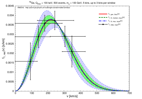
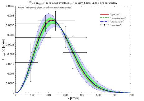
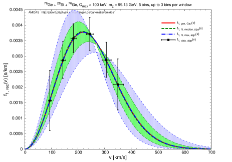
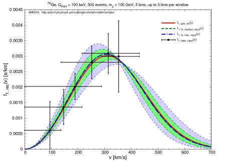
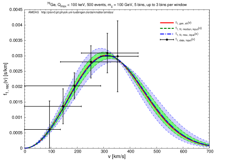
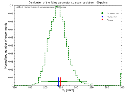
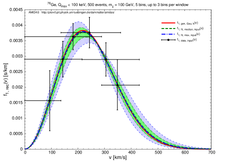
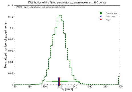
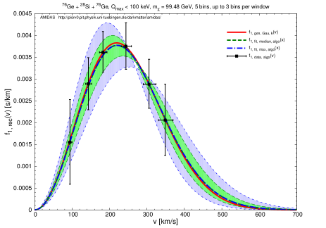
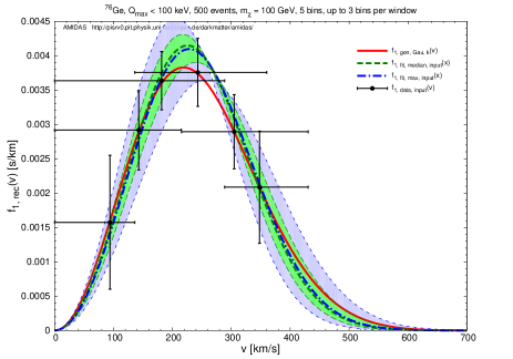
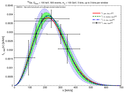
In Fig. 1(a), we show the reconstructed simple Maxwellian velocity distribution function for an input WIMP mass of GeV with a target. Here the flat distribution given by Eq. (37) for the fitting parameter has been used. The black crosses are the velocity distribution reconstructed by Eqs. (15) and (14): the vertical error bars show the square roots of the diagonal entries of the covariance matrix given in Eq. (25) (i.e. given in Eq. (30)) and the horizontal bars indicate the sizes of the windows used for estimating , respectively. The solid red curve is the generating simple Maxwellian velocity distribution with an input value of km/s. While the dashed green curve indicates the reconstructed simple Maxwellian velocity distribution with the fitting parameter given by the median value of all simulated experiments, the dash–dotted blue curve indicates the reconstructed simple Maxwellian velocity distribution with which maximizes defined in Eq. (LABEL:eqn:P_Bayesian_median).
(a) (b)
(a) (b)
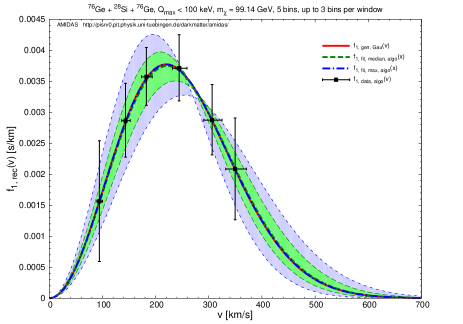
Meanwhile, the light–green (light–blue) area shown here indicate the statistical uncertainty bands of the Bayesian reconstructed velocity distribution function, which has been determined as follows. After scanning the reconstructed fitting parameter obtained from all simulated experiments and ordering according to their values defined in Eq. (LABEL:eqn:P_Bayesian_median) descendingly, we can not only determine the point which maximizes (labeled with the subscript “max” in our plots444 Note that the subscript “input” in Figs. 1 and 2 indicate that the WIMP mass needed in Eqs. (15) and (14) has been given as the input WIMP mass; whereas, the subscript “algo” in Figs. 3 and 4 indicate that the WIMP mass is reconstructed by the algorithmic procedure developed in Ref. [6]. ), but also the smallest and largest values of the first 68.27% (95.45%) of all these reconstructed ’s. We then use the smallest (largest) value of the first 68.27% (95.45%) reconstructed ’s to give the lower (upper) boundaries of the Bayesian reconstructed velocity distribution function. This means that all of the velocity distributions with ’s which give the largest 68.27% (95.45%) values should be in the light–green (light–blue) areas.
| Input: simple Maxwellian velocity distribution | ||||||
| Reconstruction: simple Maxwellian velocity distribution | ||||||
| Parameter | WIMP mass | Prob. dist. | Max. | Median | 1 range | 2 range |
| [km/s] | Input | Flat | 218.8 | [207.6, 231.4] | [196.4, 252.4] | |
| Gaussian | 221.6 | [211.8, 231.4] | [203.4, 245.4] | |||
| Reconst. | Flat | 220.2 | [202.0, 239.8] | [185.2, 267.8] | ||
| Gaussian | 220.2 | [209.0, 237.0] | [195.0, 255.2] | |||
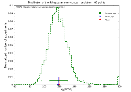
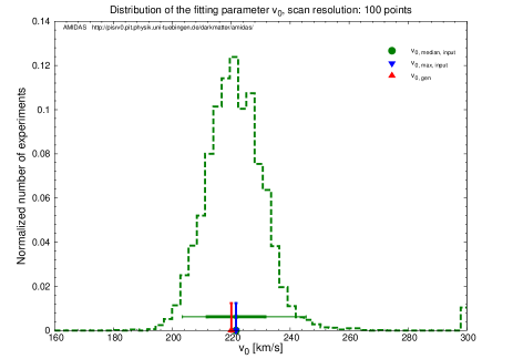
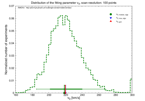
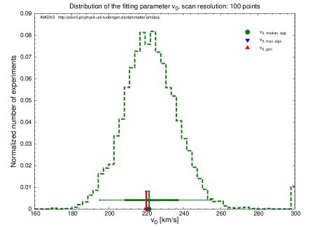
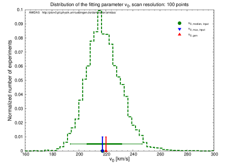
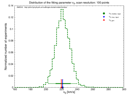
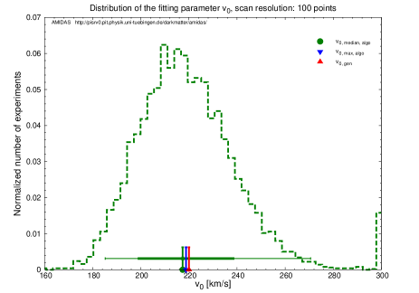
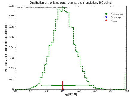
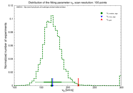
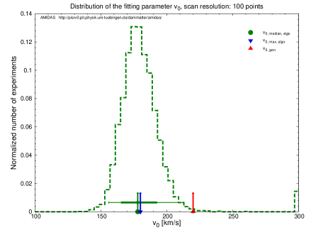
On the other hand, Fig. 1(b) shows the distribution of the Bayesian reconstructed fitting parameter in all simulated experiments. The red vertical line indicates the true (input) value of , which has been labeled with the subscript “gen”. The green vertical line indicates the median value of the simulated results, whereas the blue one indicates the value which maximizes . In addition, the horizontal thick (thin) green bars show the ranges of the reconstructed results555 Note that the ranges given here mean that, according to the order of the reconstructed values of along and centered at their median value , 68.27% (95.45%) of the reconstructed values in the simulated experiments are in this range. . Note that the bins at km/s and km/s are “overflow” bins, which contain also the experiments with the best–fit value of either km/s or km/s.
In Figs. 1, it can be seen clearly that, without a prior knowledge about the Solar Galactic velocity, one could in principle pin down the parameter very precisely with statistical uncertainties of only km/s (see Table 2). Moreover, by using the Bayesian reconstruction of the one–dimensional velocity distribution function, the large (1) statistical uncertainty given by Eq. (30) can be reduced significantly: the band of the 2 statistical uncertainty would be approximately equal to or even smaller than the (solid black) vertical 1 uncertainty bars!
Furthermore, in Figs. 2 we consider the case with a rough prior knowledge about the Solar Galactic velocity . It has been found that, firstly, by using a Gaussian probability distribution for with a 1 uncertainty of 20 km/s, one could reduce the statistical uncertainties on the Bayesian reconstructed parameter to km/s (see Table 2). Secondly and more importantly, although an expectation value of km/s, which differs (slightly) from the true (input) one, is used, the value of the fitting parameter could still be pinned down precisely with a tiny systematic deviation ( 2 km/s).
(a) (b)
(a) (b)
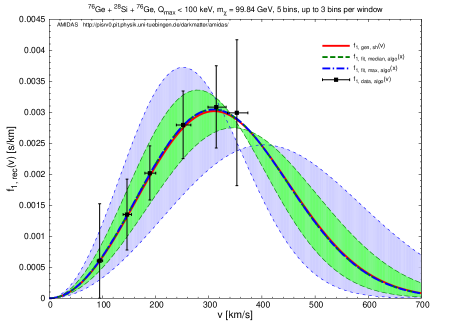
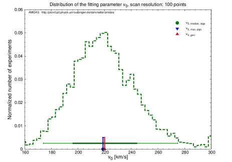
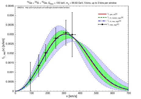
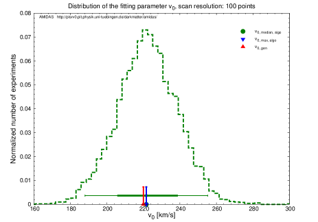
In Figs. 3 and 4, we consider the case that the WIMP mass needed in Eqs. (15) and (16) is reconstructed by the algorithmic procedure developed in Ref. [6] with a target and a second target. Note that, while the vertical bars show the 1 statistical uncertainties estimated by Eq. (30) taking into account an extra contribution from the 1 statistical uncertainty on the reconstructed WIMP mass, the horizontal bars shown here indicate the 1 statistical uncertainties on the estimates of given in Eq. (15) due to the uncertainty on the reconstructed WIMP mass; the statistical and systematic uncertainties due to estimating of have been neglected here.
It can be seen that, due to the extra statistical fluctuation on the reconstructed WIMP mass [6] and in turn the uncertainty on the estimated (the horizontal bars in the left frames), the statistical uncertainties on the Bayesian reconstructed with both of the flat and the Gaussian probability distributions become % to % larger. However, same as the case with an input WIMP mass, the use of the Gaussian probability distribution can not only reduce the statistical uncertainty on significantly and therefore improve the Bayesian reconstructed velocity distribution, but also alleviate the “imprecisely” expected value of .
In Table 2, we list the reconstructed results of for all four considered cases with the simple Maxwellian velocity distribution as well as the uncertainty ranges of the median values of . It would be worth to emphasize that, the statistical uncertainties shown in Figs. 2 and 4 are (much) smaller than the input uncertainty on the expectation value of of 20 km/s.
3.2 Shifted Maxwellian velocity distribution
| Input: shifted Maxwellian velocity distribution | |||||
| Fitting model | Parameter | Input/theoretical value | Scanning range | Expectation value | 1 uncertainty |
| Simple | [km/s] | [160, 400] | 280 | 40 | |
| 1–para. shifted | [km/s] | 220 | [160, 300] | 230 | 20 |
| Shifted | [km/s] | 220 | [160, 300] | 230 | 20 |
| [km/s] | 231 | [160, 300] | 245 | 20 | |
| Variated shifted | [km/s] | 220 | [160, 300] | 230 | 20 |
| [km/s] | 11 | [, 80] | 15 | 20 | |
By taking into account the orbital motion of the Solar system around our Galaxy as well as that of the Earth around the Sun, a more realistic shifted Maxwellian velocity distribution of halo WIMPs has been given by [1, 5]:
| (41) |
Here is the time-–dependent Earth’s velocity in the Galactic frame [17, 1]:
| (42) |
with June 2nd is the date on which the velocity of the Earth relative to the WIMP halo is maximal666 In our simulations, the time dependence of the Earth’s velocity in the Galactic frame, the second term of , will be ignored, i.e. is used. .
In Table 3, we list the input setup for the shifted Maxwellian velocity distribution used for generating WIMP signals as well as the theoretically estimated values, the scanning ranges, the expectation values of and the 1 uncertainties on the fitting parameters used for different fitting velocity distribution functions.
3.2.1 Simple Maxwellian velocity distribution
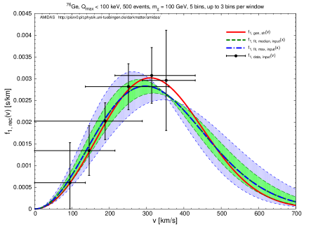
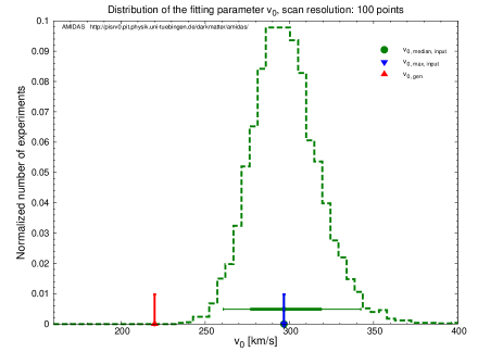
(a) (b)
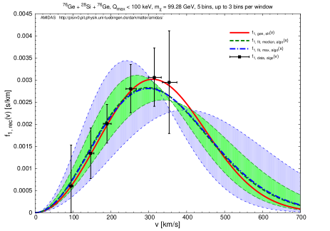
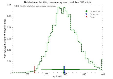
(c) (d)
(a) (b)
(c) (d)
| Input: shifted Maxwellian velocity distribution | ||||||
| Reconstruction: simple Maxwellian velocity distribution | ||||||
| Parameter | WIMP mass | Prob. dist. | Max. | Median | 1 range | 2 range |
| [km/s] | Input | Flat | 296.8 | [277.6, 318.4] | [260.8, 342.4] | |
| Gaussian | 294.4 | [280.0, 308.8] | [265.6, 323.8] | |||
| Reconst. | Flat | 299.2 | [265.6, 337.6] | [236.8, 383.2] | ||
| Gaussian | 294.4 | [268.0, 320.8] | [241.6, 347.2] | |||
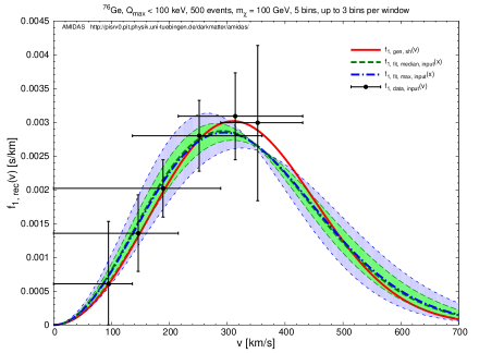
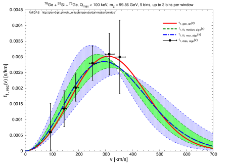
We consider first the simplest case of the simple Maxwellian velocity distribution function with the unique fitting parameter to fit the reconstructed–input data points given by Eqs. (14) and (25).
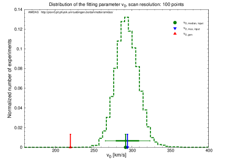
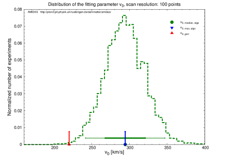
As in Sec. 3.1.1, in Figs. 5 we use first the flat probability distribution for the fitting parameter with either the precisely known (input) (upper) or the reconstructed (lower) WIMP mass, respectively. Figs. 5(a) and (c) show clearly that, although an “improper” choice for the fitting velocity distribution function and a simple flat probability distribution for (i.e. without any prior knowledge about ) have been used, the 1 statistical uncertainty bands of the reconstructed WIMP velocity distribution function could in principle still cover the true (input) distribution. More precisely and quantitatively, the deviations of the peaks of the reconstructed velocity distributions from that of the true (input) one are only km/s. Note that the 1 statistical uncertainty on the reconstructed fitting parameter is km/s or even km/s (see Table 4).
However, our simulations show also that, with an “improper” assumption about the fitting velocity distribution function, one would obtain an “unexpected” result for the fitting parameter : 2.5 (with the reconstructed WIMP mass, Fig. 5(d)) to 4 (with the input WIMP mass, Fig. 5(b)) deviations of the reconstructed Solar Galactic velocity from the theoretical estimate of km/s. Such observation would indicate clearly that our initial assumption about the fitting velocity distribution function would be incorrect or at least need to be modified.
Moreover, in Figs. 6 we assume that a rough prior knowledge about the Solar Galactic velocity exists and use the Gaussian probability distribution for with an expectation value of km/s and a 1 uncertainty of 40 km/s. As observed in Sec. 3.1.1, with a prior knowledge about the fitting parameter , one could reconstruct the velocity distribution function better: the statistical uncertainties on could be reduced to %. Additionally, the reconstructed 1 statistical uncertainties on with both of the input and the reconstructed WIMP masses are much smaller than the input 1 value of 40 km/s.
In Table 4, we list the reconstructed values of for all four considered cases with the simple Maxwellian velocity distribution as well as the uncertainty ranges of the median values of .
3.2.2 One–parameter shifted Maxwellian velocity distribution
(a) (b)
(c) (d)
(a) (b)
(c) (d)
In the previous Sec. 3.2.1, we have found that, by assuming (improperly) the simple Maxwellian velocity distribution , in both cases with and without an expectation value of the fitting parameter , one would obtain a much higher reconstruction result: km/s, which is 2 to 4 apart from the theoretical estimate of km/s. This observation implies the need of a more suitable fitting velocity distribution function. Hence, as the second trial, we consider now the use of the shifted Maxwellian velocity distribution given in Eq. (41) with only one fitting parameter, i.e. the Solar Galactic velocity . In this case, we fix simply that
| (43) |
and neglect the time–dependence of .777 Note that hereafter we use to denote the “one–parameter” shifted Maxwellian velocity distribution function, in order to distinguish this from the “original” one given in Eq. (41) with and as two independent fitting parameters.
In Figs. 7, we consider first the flat probability distribution for the fitting parameter with either the precisely known (input) (upper) or the reconstructed (lower) WIMP mass, respectively. It can be seen clearly that, with a more suitable assumption about the fitting function, one could indeed reconstruct the WIMP velocity distribution much closer to the true (input) one. Although no prior knowledge about is used, this most important characteristic parameter could in principle be pinned down very precisely: the difference between the median values of the reconstructed and the true (input) one would be km/s (see also Table 5).
In addition, with the input WIMP mass, the statistical uncertainties on the reconstructed are only km/s. Even with the reconstructed WIMP mass, the statistical uncertainties could still be limited as small as only km/s. It would be worth to emphasize that, compared to the uncertainty on the astronomical measurement of of km/s (or probably larger), the result offered by our Bayesian reconstruction method would be a pretty precise estimate and could help us to confirm the astronomical measurement of .
Moreover, in Figs. 8 we give the reconstruction results with the Gaussian probability distribution for with an expectation value of km/s and a 1 uncertainty of 20 km/s. As summarized in Table 5, with a prior knowledge of the parameter , the statistical uncertainties could be reduced significantly to be 70%. Remind here that the expectation value of the Gaussian probability distribution of has been set as km/s, a bit different from the input value. Nevertheless, our simulations show that this “artificial” (systematic) error could be corrected in our reconstruction process for .
In Table 5, we list the reconstructed results of for all four considered cases with the one–parameter shifted Maxwellian velocity distribution as well as the uncertainty ranges of the median values of .
| Input: shifted Maxwellian velocity distribution | ||||||
| Reconstruction: one–parameter shifted Maxwellian velocity distribution | ||||||
| Parameter | WIMP mass | Prob. dist. | Max. | Median | 1 range | 2 range |
| [km/s] | Input | Flat | 217.4 | [206.2, 231.4] | [193.6, 246.8] | |
| Gaussian | 221.6 | [213.2, 231.4] | [203.4, 239.8] | |||
| Reconst. | Flat | 218.8 | [196.4, 244.0] | [174.0, 274.8] | ||
| Gaussian | 221.6 | [206.2, 238.4] | [188.0, 255.2] | |||
3.2.3 Shifted Maxwellian velocity distribution
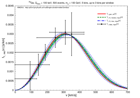
(a) (b)
(c) (d)
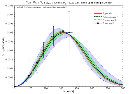
(a) (b)
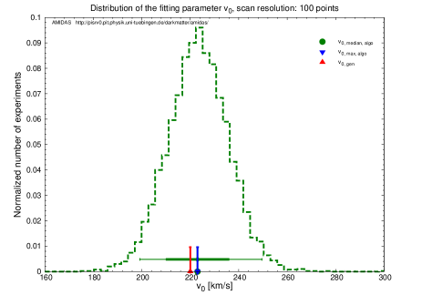
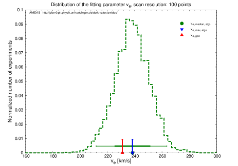
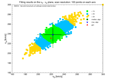
(c) (d)
Now we release the fixed relation between and given in Eq. (43) and consider the reconstruction of these two parameters simultaneously and independently. In addition, we assume here that, from the (naive) trials with the simple and one–parameter shifted Maxwellian velocity distributions done previously, one could already obtain a rough idea about the shape of the velocity distribution of halo WIMPs. This information would in turn give us the prior knowledge about the expectation values of the Solar and Earth’s Galactic velocities and . Hence, we consider here only the Gaussian probability distribution for both fitting parameters with expectation values of km/s and km/s and a common 1 uncertainty of 20 km/s (see Table 3)888 Remind that both of the expectation values of the fitting parameters and differ slightly from the true (input) values. Note also that the time–dependence of the Earth’s Galactic velocity is ignored here and is thus treated as a time–independent fitting parameter. .
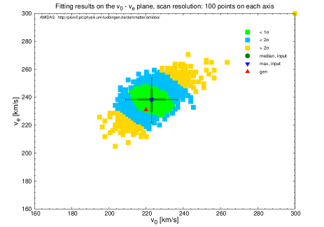
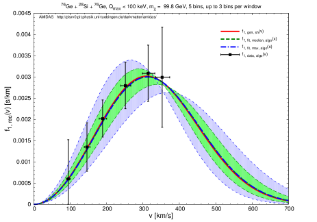
In Fig. 9(a), we show the reconstructed shifted Maxwellian velocity distribution function as well as the statistical uncertainty bands. Here the true (input) WIMP mass has been used. Comparing to Fig. 8(a), it can be seen clearly that, with a prior knowledge about the Solar and Earth’s Galactic velocities and , one could in principle reconstruct the velocity distribution function with two fitting parameters more precisely: the statistical uncertainty bands are much thinner and the deviations of and are only a few km/s (see also Table 6)999 Note however that, for using velocity distributions with two or more fitting parameters without constraints on these parameters (i.e. the use of the “flat” probability distribution), the distribution of the reconstructed results by our Bayesian analysis would be pretty wide, a part of them would even be on the boundary of the scanning ranges of these parameters. .
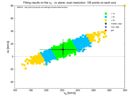
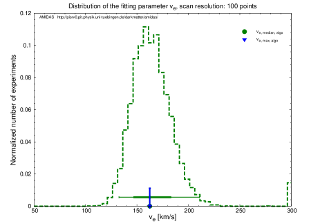
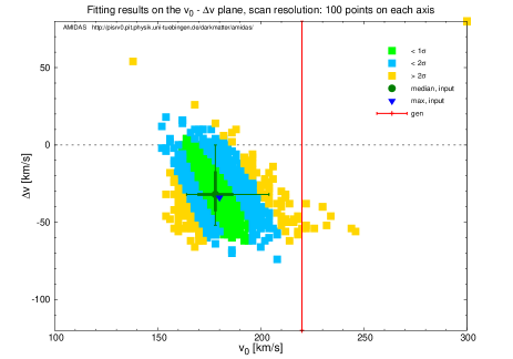
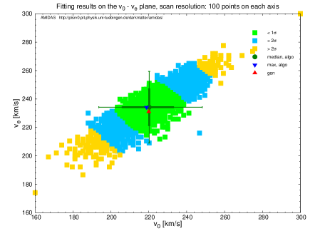
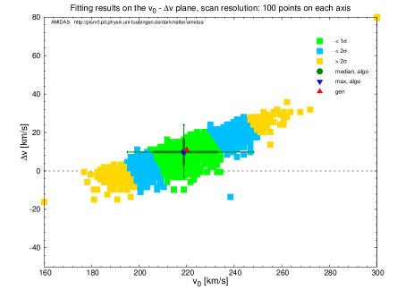
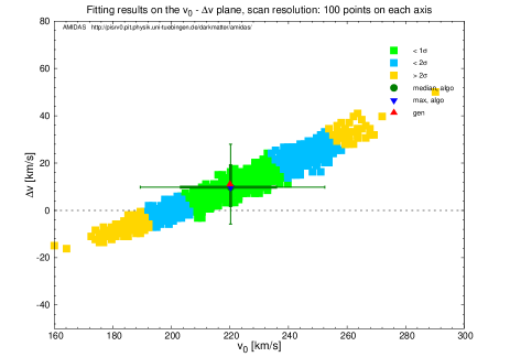
Fig. 9(b) shows the distribution of the Bayesian reconstructed fitting parameter and in all simulated experiments on the plane. The light–green (light–blue, gold) points indicate the areas of the reconstructed combination of and . Note here that these areas are determined according to the descending order of the values of the reconstructed combination of and . This means that the light–green (light–blue, gold) areas are the reconstructed combinations of and which give the largest 68.27% (95.45%) values in all of the simulated experiments.
Moreover, the red upward–triangle indicates the input values of and , which has been labeled with the subscript “gen”. The green disk shows the median values of the simulated results, whereas and blue downward–triangle the point which maximizes . In addition, the thick (thin) green crosses show the (68.27% (95.45%)) ranges of the reconstructed results according to the order of the reconstructed values of or along (centered at their median values or ).
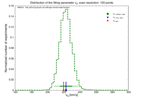
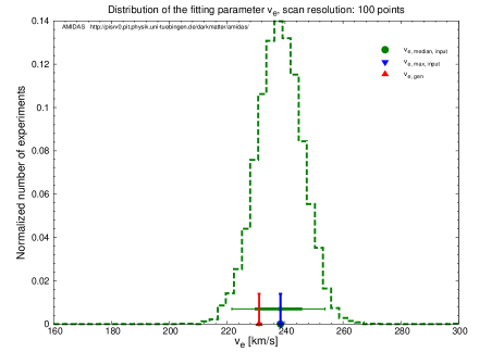
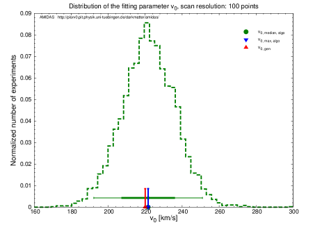
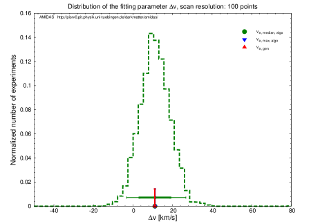
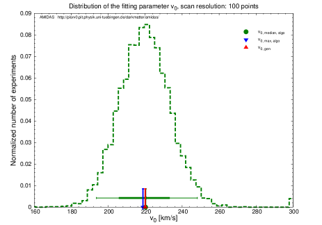
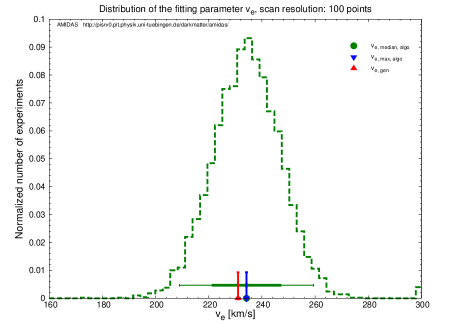
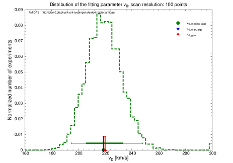
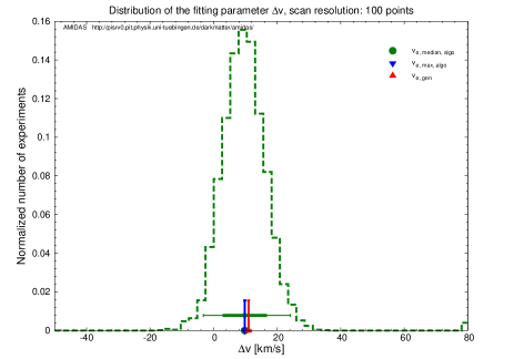
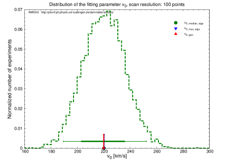
Additionally, in Figs. 9(c) and (d), we give the distributions of the Bayesian reconstructed fitting parameters and as well as the statistical uncertainty ranges on the and axes separately. Note here that we project all reconstructed combinations of on the or axis. Comparing Fig. 9(c) to Fig. 8(b), it can be found that, while the deviations of are a little bit larger then the results with the “one–parameter” fitting velocity distribution, the statistical uncertainties are reduced to 70% (see Table 6 and Table 5).
| Input: shifted Maxwellian velocity distribution | ||||||
| Reconstruction: shifted Maxwellian velocity distribution | ||||||
| Parameter | WIMP mass | Prob. dist. | Max. | Median | 1 range | 2 range |
| [km/s] | Input | Gaussian | 223.0 | [216.0, 230.0] | [209.0, 237.0] | |
| Reconst. | Gaussian | 223.0 | [210.4, 235.6] | [199.2, 249.6] | ||
| [km/s] | Input | Gaussian | 238.4 | [230.0, 245.4] | [221.6, 253.8] | |
| Reconst. | Gaussian | 238.4 | [225.8, 251.0] | [211.8, 263.6] | ||
As a comparison, in Figs. 10 we use the reconstructed WIMP mass. Fig. 10(b) shows that, as expected, the distribution of and on the plane becomes wider and extends toward the directions of higher (lower)– and higher (lower)–. Nevertheless, the “best–fit” combination of them which maximizes as well as the median values of and consistant very well with the true (input) values.
In Table 5, we list the reconstructed results of and with the shifted Maxwellian velocity distribution as well as the uncertainty ranges of the median values.
3.2.4 Variated shifted Maxwellian velocity distribution
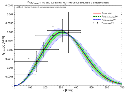
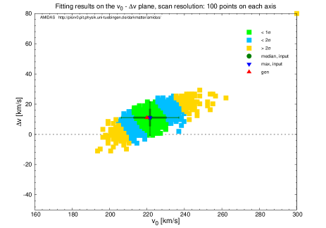
(a) (b)
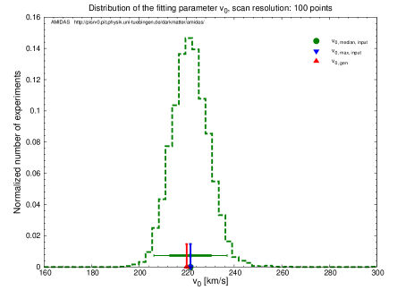
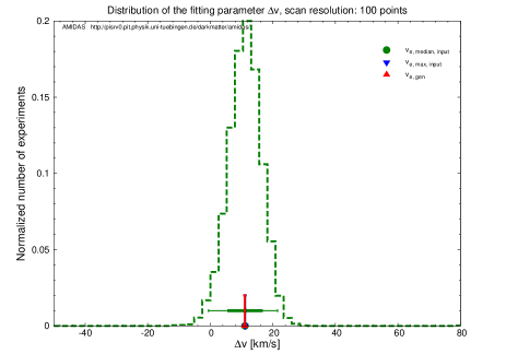
(c) (d)
(a) (b)
(c) (d)
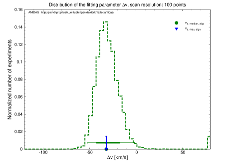
In the previous Sec. 3.2.3, it has been found that, by using the shifted Maxwellian velocity distribution given in Eq. (41) with two fitting parameters: and , one could reconstruct the ( statistical uncertainty bands of the) velocity distribution function as well as pin down the Solar Galactic velocity pretty precisely. However, as shown in Figs. 9(d) and 10(d), the deviations of the reconstructed Earth’s Galactic velocity from the true (input) value seem to be (much) larger than the deviations of the reconstructed . This might be caused by the strong (anti–)correlation between and . Hence, we consider now a variation of the shifted Maxwellian distribution function, in the hope that this pretty large systematic deviation of could be reduced.
We rewrite the shifted Maxwellian velocity distribution given in Eq. (41) to the following “variated” form:
| (44) |
where
| (45) |
is the difference between and .101010 As in the previous Sec. 3.2.3, the time–dependence of the Earth’s Galactic velocity is ignored here and is thus treated as a time–independent fitting parameter.
| Input: shifted Maxwellian velocity distribution | ||||||
| Reconstruction: variated shifted Maxwellian velocity distribution | ||||||
| Parameter | WIMP mass | Prob. dist. | Max. | Median | 1 range | 2 range |
| [km/s] | Input | Gaussian | 221.6 | [213.2, 230.0] | [206.2, 237.0] | |
| Reconst. | Gaussian | 221.6 | [207.6, 235.6] | [192.2, 251.0] | ||
| [km/s] | Input | Gaussian | 11.1 | [5.9, 16.3] | [, 21.5] | |
| Reconst. | Gaussian | 11.1 | [3.3, 18.9] | [, 26.7] | ||
As in the previous Sec. 3.2.3, we assume here that, we have already a rough idea about the shape of the velocity distribution of halo WIMPs, and thus the prior knowledge about the expectation values of the (difference between the) Solar and Earth’s Galactic velocities and . Hence, we consider here only the Gaussian probability distribution for both of the fitting parameters with expectation values of km/s and km/s and a common 1 uncertainty of 20 km/s (see Table 3). Two cases with both of the true (input) and the reconstructed WIMP masses have been considered.
By comparing Figs. 11 to Figs. 9 and Figs. 12 to Figs. 10, it can be seen obviously that the reconstructed velocity distribution function could indeed match the true (input) one much precisely, with however (slightly) wider statistical uncertainty bands. The systematic deviations of both fitting parameters from the true (input) values would also be much smaller than those given in the case. This implies importantly that, the use of our variated shifted velocity distribution function given in Eq. (44) could indeed offer an estimate of the Earth’s Galactic velocity with a much higher precision. Such a trick would be helpful to improve the estimation(s) of the Earth’s Galactic velocity (and/or other fitting parameter(s)).
Note however that, as shown in Tables 6 and 7, by using the variated shifted Maxwellian velocity distribution, the statistical uncertainties on the reconstructed would be 10% larger. Meanwhile, from Eq. (45) the statistical uncertainty on can be estimated by111111 Since, according to Eq. (45), for a fixed value of two fitting parameters and should be “anti–correlated”.
| (46) | |||||
Then, according to the results given in Table 7, the statistical uncertainties on would be maximal enlarged, whereas the systematic deviation of is much smaller.
In Table 7, we list the reconstructed results of and with the variated shifted Maxwellian velocity distribution as well as the uncertainty ranges of the median values.
3.3 Modified Maxwellian velocity distribution
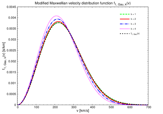
In this subsection, we consider another recently often used theoretical one–dimensional WIMP velocity distribution function. In Refs. [18, 10], a modification of the simple Maxwellian velocity distribution in Eq. (40) has been suggested:
| (47) |
Here is the maximal cut-–off velocity of and is the normalization constant depending on the value of the power index .
| Input: modified Maxwellian velocity distribution | |||||
| Fitting model | Parameter | Input/theoretical value | Scanning range | Expectation value | 1 uncertainty |
| Simple | [km/s] | [160, 300] | 230 | 20 | |
| 1–para. shifted | [km/s] | [100, 300] | 200 | 40 | |
| Shifted | [km/s] | [100, 300] | 200 | 40 | |
| [km/s] | [50, 300] | 200 | 40 | ||
| Variated shifted | [km/s] | [100, 300] | 200 | 40 | |
| [km/s] | [, 80] | 40 | |||
| Modified | [km/s] | 220 | [160, 300] | 230 | 20 |
| 2 | [0.5, 3.5] | 1 | 0.5 | ||
In Fig. 13, we give the normalized modified Maxwellian velocity distribution function with a common value of the Solar Galactic velocity km/s and different power indices : (dashed light–green), (solid red), (dash–dotted blue) and (dotted magenta). As a comparison, the simple Maxwellian velocity distribution with km/s is also given as the short–dashed black curve.
In Table 8, we list the input setup for the modified Maxwellian velocity distribution used for generating WIMP signals as well as the theoretically estimated values, the scanning ranges, the expectation values of and the 1 uncertainties on the fitting parameters used for different fitting velocity distribution functions.
3.3.1 Simple Maxwellian velocity distribution

(a) (b)

(c) (d)
(a) (b)
(c) (d)
As in Sec. 3.2, we start to fit to the reconstructed–input data points given by Eqs. (14) and (25) with the simple Maxwellian velocity distribution function .
In Figs. 14, we use first the flat probability distribution for the fitting parameter with either the precisely known (input) (upper) or the reconstructed (lower) WIMP mass, respectively. As shown in Figs. 1 and 3, although prior knowledge about the Solar Galactic velocity is absent, one could in principle pin down the fitting parameter very precisely with systematic deviations of only a few km/s and statistical uncertainties of only km/s and km/s.
| Input: modified Maxwellian velocity distribution | ||||||
| Reconstruction: simple Maxwellian velocity distribution | ||||||
| Parameter | WIMP mass | Prob. dist. | Max. | Median | 1 range | 2 range |
| [km/s] | Input | Flat | 217.4 | [204.8, 228.6] | [195.0, 253.8] | |
| Gaussian | 218.8 | [210.4, 230.0] | [202.0, 246.8] | |||
| Reconst. | Flat | 218.8 | [199.2, 238.4] | [185.2, 270.6] | ||
| Gaussian | 220.2 | [206.2, 235.6] | [193.6, 256.6] | |||
In Figs. 15, we use the Gaussian probability distribution for with an expectation value of km/s and a 1 uncertainty of 20 km/s. As summarized in Table 9, the statistical uncertainties on the reconstructed could now in principle be reduced by % to %. In addition, even with the reconstructed WIMP mass and thus a larger statistical fluctuation, the 1 statistical uncertainties shown in Figs. 15 are (much) smaller than the given uncertainty on the expectation value of (20 km/s). Moreover, although an expectation value of km/s, which differs (slightly) from the true (input) one, is used, the value of the fitting parameter could still be pinned down precisely with a negligible systematic deviation.
Furthermore, remind here that, either, as shown in Figs. 14, two reconstructed (dashed green and dash-dotted blue) velocity distribution functions match the true (input) (solid red) one very well, but the reconstructed Solar Galactic velocity would shift slightly away from the true (input) value, or, as shown in Figs. 15, could be determined very precisely, but the reconstructed velocity distribution functions would differ slightly from the true (input) one. This is because of the fact that we have artificially used an input value of and, as shown in Fig. 13, the modified Maxwellian velocity distribution function with is slightly different from the simple Maxwellian distribution.
In Table 9, we list the reconstructed results of for all four considered cases with the simple Maxwellian velocity distribution as well as the uncertainty ranges of the median values of .
3.3.2 One–parameter shifted Maxwellian velocity distribution
(a) (b)

(c) (d)
(a) (b)
(c) (d)
| Input: modified Maxwellian velocity distribution | ||||||
| Reconstruction: one–parameter shifted Maxwellian velocity distribution | ||||||
| Parameter | WIMP mass | Prob. dist. | Max. | Median | 1 range | 2 range |
| [km/s] | Input | Flat | 162.0 | [152.0, 170.0] | [146.0, 188.0] | |
| Gaussian | 162.0 | [154.0, 172.0] | [148.0, 188.0] | |||
| Reconst. | Flat | 162.0 | [148.0, 176.0] | [138.0, 198.0] | ||
| Gaussian | 164.0 | [150.0, 178.0] | [138.0, 200.0] | |||
Now, as a comparison of Sec. 3.3.1, we consider as the next trail the reconstruction with the one–parameter shifted Maxwellian velocity distribution function to fit the modified simple Maxwellian velocity distribution.
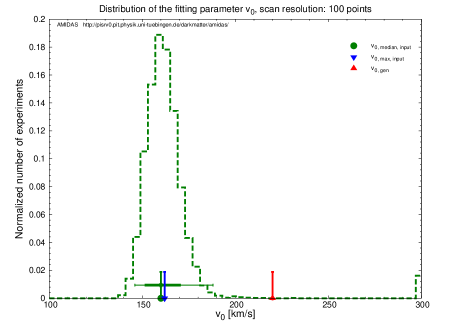
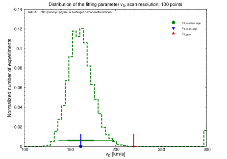
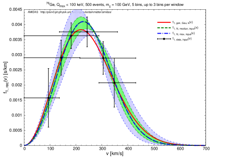
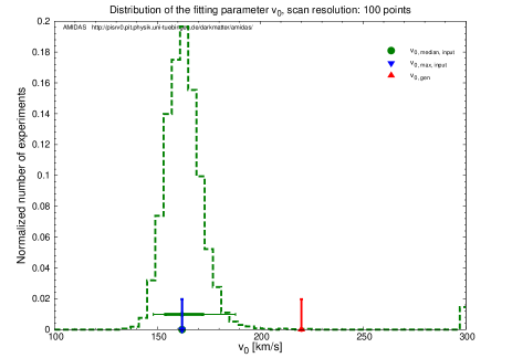
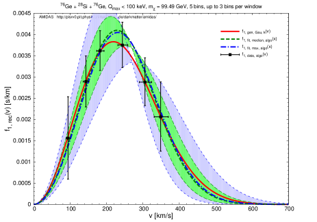
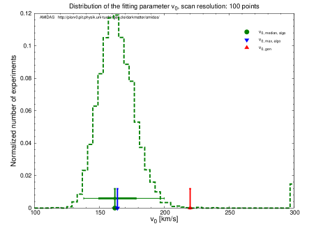
As usual, in Figs. 16 we use first the flat probability distribution for the fitting parameter with either the precisely known (input) (upper) or the reconstructed (lower) WIMP mass, respectively. It can be seen that, firstly, although the statistical uncertainty bands could still cover the true (input) velocity distribution (somehow well), the systematic deviations of the peaks of the reconstructed velocity distributions from that of the true (input) one would be km/s. The comparisons between reconstructed results shown in Figs. 16(a) and (c) to Figs. 14(a) and (c) could indicate a high probability of the improper assumption of the fitting (one–parameter) shifted Maxwellian velocity distribution.
Moreover, Figs. 16(b) and (d) (see also Table 10) show clearly 4 to even 6 deviations of the reconstructed from the true (input) value of km/s. As discussed in Sec. 3.2.1, this observation implies also an improper use of the (one–parameter) shifted Maxwellian velocity distribution as our fitting function.
In Figs. 17, we use the Gaussian probability distribution for with a slightly smaller expectation value of km/s and a 1 uncertainty of 40 km/s. In contrast to our observations presented before, for this case the use of the Gaussian probability distribution would not reduce the statistical uncertainties for both cases with the true (input) and the reconstructed WIMP masses (see Table 10). This would be caused by the large difference between the given expectation value and the (theoretically estimated) most suitable one of the parameter (175 km/s, see Table 8). This would indicate that, in practical use of our Bayesian reconstruction method, some trial–and–error tests for determining a more suitable expectation value of (and the other fitting parameters) would be necessary and could then improve the fitting results.
In Table 10, we list the reconstructed results of for all four considered cases with the one–parameter shifted Maxwellian velocity distribution as well as the uncertainty ranges of the median values of .
3.3.3 Shifted Maxwellian velocity distribution
(a) (b)
(c) (d)
(a) (b)
(c) (d)
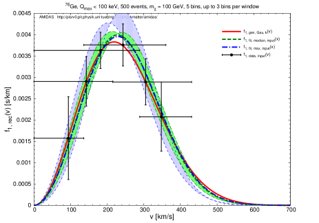
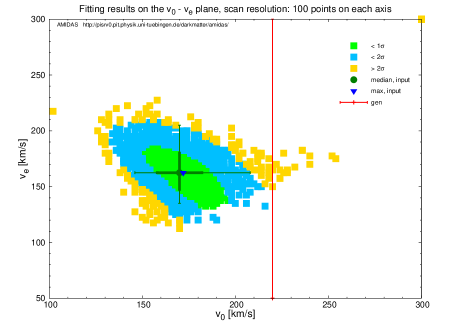
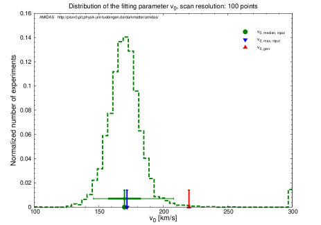
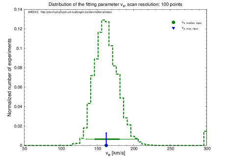
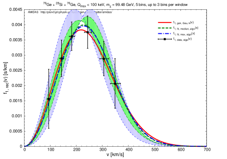
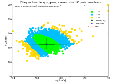
As in Sec. 3.2.3, we release now the fixed relation between and given in Eq. (43) and consider the reconstruction of these two parameters simultaneously and independently. In addition, we also assume here that, from the (naive) trials with the simple and one–parameter shifted Maxwellian velocity distributions done previously, one could already obtain a rough idea about the shape of the velocity distribution of halo WIMPs as well as expectation values of the Solar and Earth’s Galactic velocities and . Hence, we consider here only the Gaussian probability distribution for both fitting parameters with a common expectation value of km/s and a common 1 uncertainty of 40 km/s (see Table 8). Note also that, after some trial–and–error tests, we set the scanning ranges of and as km/s and km/s.
In Figs. 18, we consider first the case with the true (input) WIMP mass. As observed in Sec. 3.3.2, although the (low–velocity parts of the) statistical uncertainty bands could cover the true (input) velocity distribution, the systematic deviations of the peaks of the reconstructed velocity distributions from that of the true (input) one would be km/s (a little bit better then results shown in Figs. 16(a) and (c)). Moreover, Figs. 18(c) and (d) show deviations of the reconstructed values of and from the true (input, estimated) values of km/s and km/s. Additionally, the best–fit value of is now even ( km/s) smaller than the best–fit value of . Hence, as discussed in Sec. 3.3.2, this observation (combined with the results given in Sec. 3.3.2) would indicate a high probability of the improper assumption of the fitting shifted Maxwellian velocity distribution. Moreover, in Figs. 19 we show our simulations with the reconstructed WIMP mass. The statistical uncertainties on and would be 10% to 50% enlarged.
| Input: modified Maxwellian velocity distribution | ||||||
| Reconstruction: shifted Maxwellian velocity distribution | ||||||
| Parameter | WIMP mass | Prob. dist. | Max. | Median | 1 range | 2 range |
| [km/s] | Input | Gaussian | 172.0 | [158.0, 182.0] | [146.0, 208.0] | |
| Reconst. | Gaussian | 172.0 | [156.0, 188.0] | [140.0, 214.0] | ||
| [km/s] | Input | Gaussian | 162.5 | [147.5, 180.0] | [135.0, 205.0] | |
| Reconst. | Gaussian | 162.5 | [147.5, 182.5] | [132.5, 210.6] | ||
Figs. 18 and 19 as well as Table 11 show that one could fit an improper model to experimental data (somehow) well with combinations of special, probably unusual values of the fitting parameters. On one hand, the reconstructed results could offer us (rough) information about the (shape of the) velocity distribution of Galactic WIMPs. On the other hand, however, the observation that the reconstructed values of and are to even different from our (theoretically) expected values would indicate evidently the improper assumption about the fitting velocity distribution function.
In Table 11, we list the reconstructed results of and with the shifted Maxwellian velocity distribution as well as the uncertainty ranges of the median values.
3.3.4 Variated shifted Maxwellian velocity distribution
(a) (b)
(c) (d)
(a) (b)
(c) (d)
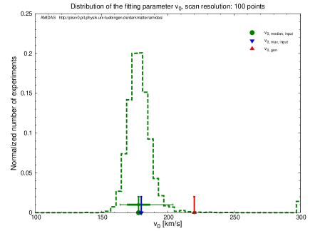
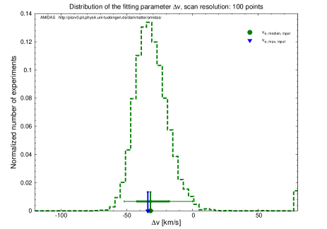
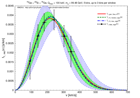
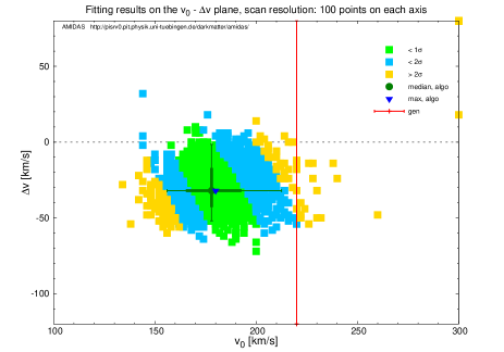
As in Sec. 3.2.4, in order to correct the systematic deviations of the results given with the shifted Maxwellian velocity distribution function in Eq. (41), we consider here the use of its variation given in Eq. (44). As previously, we consider here only the Gaussian probability distribution for both fitting parameters and , with a common 1 uncertainty of 40 km/s. Moreover, according to the fitting results given in Sec. 3.3.3 and some trial–and–error tests, we set km/s and km/s as the expectation values as well as km/s and km/s as the scanning ranges.
Comparing Figs. 20 to Figs. 18, it can be seen clearly that the use of the variated shifted Maxwellian velocity distribution could indeed offer a more reasonable and preciser reconstruction: not only that the ( statistical uncertainty bands of the) reconstructed velocity distribution functions can match the true (input) one more closer, the statistical uncertainties on is also only 70% of the uncertainties shown in Fig. 18(c). Additionally, by using Eq. (46), the upper bound of the statistical uncertainties on can be (approximately) given as: km/s, which is also maximal (approximately) equal to or even smaller than the uncertainties given in Table 11. Hence, we would like to conclude that our introduction of the variated shifted Maxwellian velocity distribution (and/or probably some other variations) could indeed be a useful trick for the practical use of our Bayesian reconstruction procedure.
| Input: modified Maxwellian velocity distribution | ||||||
| Reconstruction: variated shifted Maxwellian velocity distribution | ||||||
| Parameter | WIMP mass | Prob. dist. | Max. | Median | 1 range | 2 range |
| [km/s] | Input | Gaussian | 180.0 | [170.0, 186.0] | [164.0, 204.0] | |
| Reconst. | Gaussian | 180.0 | [166.0, 192.0] | [156.0, 212.5] | ||
| [km/s] | Input | Gaussian | [, ] | [, 0.0] | ||
| Reconst. | Gaussian | [, ] | [, ] | |||
On the other hand, in Figs. 21 we use the reconstructed WIMP mass. Comparing Figs. 21 to Figs. 20 (see also Table 12), although the width of the statistical uncertainty bands of the reconstructed velocity distribution functions as well as the statistical uncertainties on would be clearly larger, the statistical uncertainties on are approximately equal to results with the true (input) WIMP mass. Meanwhile, even for this case with the reconstructed WIMP mass, the statistical uncertainties on and are (much) smaller than the given 1 uncertainty of their Gaussian probability distributions (40 km/s).
Remind that, our simulations of the use of the variated shifted Maxwellian velocity distribution function for fitting data generated by (modified) simple Maxwellian one shown here indicates again that, by using an “improper” assumption about the fitting velocity distribution function with prior knowledge about the fitting parameters (, or ), one would still reconstruct an approximate shape of the WIMP velocity distribution; the deviations of the peaks of the reconstructed velocity distributions from that of the true (input) one could even be km/s, much smaller than the commonly used 1 uncertainty on the Solar Galactic velocity of km/s.
However, our simulations show also that, with an “improper” assumption about the fitting velocity distribution, one would obtain an “unexpected” result about each single fitting parameter. E.g. here we get 3 to 5 deviations of the reconstructed Solar Galactic velocity from the theoretical estimate (see Table 12) and large “negative” values for the difference between the Solar and Earth’s Galactic velocities. This observation indicates clearly that our initial assumption about the fitting velocity distribution function would be incorrect or at least need to be modified.
In Table 12, we list the reconstructed results of and with the variated shifted Maxwellian velocity distribution as well as the uncertainty ranges of the median values.
3.3.5 Modified Maxwellian velocity distribution

(a) (b)
(c) (d)
(a) (b)
(c) (d)
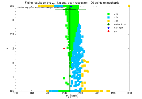
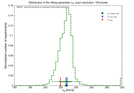
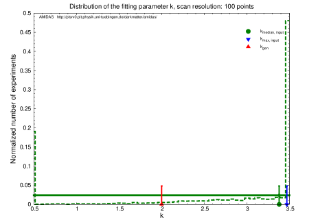
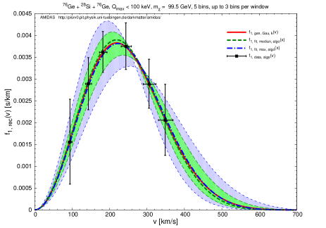
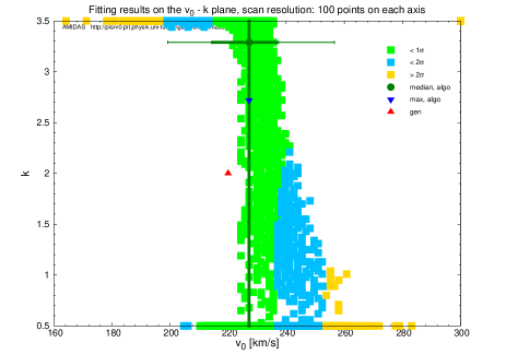
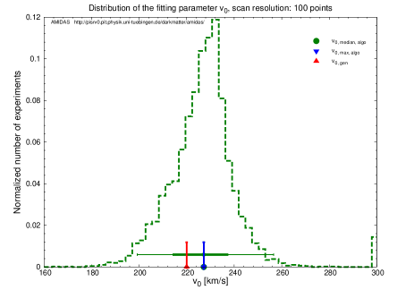
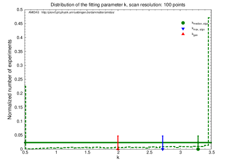
As the last tested fitting velocity distribution function with data generated by the modified Maxwellian velocity distribution given by Eq. (47), we consider now the reconstruction of the modified Maxwellian velocity distribution itself with two fitting parameters: the Solar Galactic velocity and the power index .
In Figs. 22 and 23, we use the Gaussian probability distribution for the fitting parameter with an expectation value of km/s and a 1 uncertainty of 20 km/s but the flat distribution for the parameter , with either the precisely known (input) or the reconstructed WIMP mass, respectively. Remind that, in Figs. 22(d) and 23(d) the bins at and are “overflow” bins. This means that they contain also the experiments whose best–fit values of would be either or .
First, as shown in Sec. 3.3.1, the Solar Galactic velocity could be pinned down very precisely: a small systematic deviation of 10 km/s and 1 statistical uncertainty of km/s could be achieved. However, Figs. 22(b) and (d) as well as Figs. 23(b) and (d) show that, due to the small difference between the modified Maxwellian velocity distribution with different power indices (see Fig. 13) and the large statistical fluctuation and 1 reconstruction uncertainty with only 500 WIMP events (on average), our Bayesian reconstruction of the velocity distribution would be totally non–sensitive on the second fitting parameter (power index) .
Nevertheless, the wide spread of the reconstructed power index (in particular, the high cumulative numbers in the (overflow) bin ) and, in contrast, the narrow widths of the statistical uncertainty bands of the reconstructed velocity distribution functions imply that, for reconstructing the rough information about the one–dimensional WIMP velocity distribution, a precise value of the power index would not be crucial, and the simple Maxwellian velocity distribution given in Eq. (40) would already be a good approximation121212 As described in Ref. [18], the modification of the simple Maxwellian velocity distribution function given in Eq. (47) has significant difference from the simple Maxwellian one given in Eq. (40) in the high–velocity tail. Moreover, in Refs. [19, 20], another empirical modification of the simple Maxwellian velocity distribution with also a significant difference in the high–velocity tail has been introduced. Unfortunately, our simulations presented here show that it would be impossible to distinguish these subtle modifications by our Bayesian reconstruction method (with only a few hundreds of recorded WIMP events). On the other hand, simulations with other (well–motivated) halo models and different fitting velocity distribution functions can be tested on the AMIDAS website [21, 22]. .
In Table 13, we give the reconstructed results of and with the modified Maxwellian velocity distribution as well as the uncertainty ranges of the median values. Note that, since the 1 lower and upper bounds of the median values of are already beyond our scanning range, the 2 bounds are meanless to give here.
| Input: modified Maxwellian velocity distribution | ||||||
| Reconstruction: modified Maxwellian velocity distribution | ||||||
| Parameter | WIMP mass | Prob. dist. | Max. | Median | 1 range | 2 range |
| [km/s] | Input | Gaussian | 228.6 | [218.8, 234.2] | [209.0, 246.8] | |
| Reconst. | Gaussian | 227.2 | [214.6, 237.0] | [199.2, 256.6] | ||
| Input | Flat | 3.47 | [0.5, 3.5] | |||
| Reconst. | Flat | 2.72 | [0.5, 3.5] | |||
3.4 For different WIMP masses
(a) (b)
(a) (b)
(c) (d)
(a) (b)
(c) (d)
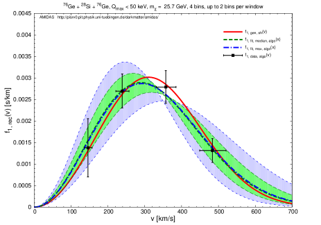
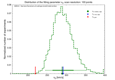
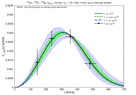
In the previous Secs. 3.1 to 3.3, we fixed the input WIMP mass as GeV. As a further test of our Bayesian reconstruction method for the one–dimensional WIMP velocity distribution, in this subsection, we consider the cases for either a light WIMP mass of GeV or a heavy WIMP mass of GeV.
Here we consider only the shifted Maxwellian velocity distribution given in Eq. (41) for generating WIMP events; three fitting functions: simple, shifted and variated shifted Maxwellian velocity distributions will be tested. All input setup and fitting parameters are the same as in Sec. 3.2 (see Table 3). Additionally, only the reconstructed WIMP mass is used.
3.4.1 For a light WIMP mass
We consider first a rather light WIMP mass of GeV. Note that, firstly, since for our tested targets and , the kinematic maximal cut–off energies given in Eq. (36) are only keV and keV, respectively, the maximal experimental cut–off energy for both targets in our simulations demonstrated here has been reduced to only keV. Secondly, since the lighter the WIMP mass, the shaper the expected recoil energy spectrum, the width of the first energy bin in Eq. (18) has been set as keV and the total number of bins has been reduced to only four bins between and (); up to two bins have been combined to a window and thus four windows () will be reconstructed131313 The last window is neglected automatically in the AMIDAS code, due to a very few expected event number in the last bin (window). 141414 It has been found that, by reducing the total number of the energy bins (and in turn that of the windows) and thus collecting more events in one bin (window), the Bayesian reconstructed velocity distribution could be improved (significantly). .
Simple Maxwellian velocity distribution
| Input: shifted Maxwellian velocity distribution | ||||||
| Reconstruction: simple Maxwellian velocity distribution | ||||||
| Parameter | WIMP mass | Prob. dist. | Max. | Median | 1 range | 2 range |
| [km/s] | Input | Flat | 296.8 | [282.4, 308.8] | [272.8, 325.6] | |
| Gaussian | 294.4 | [282.4, 304.0] | [272.8, 318.4] | |||
| Reconst. | Flat | 292.0 | [265.6, 318.4] | [246.4, 352.0] | ||
| Gaussian | 292.0 | [268.0, 311.2] | [248.8, 337.6] | |||
| Reconstruction: one–parameter shifted Maxwellian velocity distribution | ||||||
| [km/s] | Input | Flat | 220.2 | [211.8, 228.6] | [204.8, 238.4] | |
| Gaussian | 221.6 | [214.6, 228.6] | [207.6, 237.0] | |||
| Reconst. | Flat | 217.4 | [197.8, 235.6] | [183.8, 259.4] | ||
| Gaussian | 218.8 | [203.4, 234.2] | [189.4, 251.0] | |||
| Reconstruction: shifted Maxwellian velocity distribution | ||||||
| [km/s] | Input | Gaussian | 221.6 | [214.6, 228.6] | [208.7, 237.0] | |
| Reconst. | Gaussian | 218.8 | [206.2, 232.8] | [193.6, 248.2] | ||
| [km/s] | Input | Gaussian | 237.0 | [228.6, 244.0] | [220.2, 251.0] | |
| Reconst. | Gaussian | 234.2 | [221.6, 246.8] | [209.0, 259.4] | ||
| Reconstruction: variated shifted Maxwellian velocity distribution | ||||||
| [km/s] | Input | Gaussian | 221.6 | [216.0, 227.2] | [210.4, 234.2] | |
| Reconst. | Gaussian | 218.8 | [206.2, 232.8] | [195.0, 248.2] | ||
| [km/s] | Input | Gaussian | 9.8 | [5.9, 15.0] | [, 20.2] | |
| Reconst. | Gaussian | 9.8 | [3.3, 16.3] | [, 24.1] | ||
In Figs. 24 (cf. Figs. 5(c) and (d)), we use first the (improper) simple Maxwellian velocity distribution function with one parameter to fit the reconstructed–input data. As the first trial of the reconstruction of the one–dimensional WIMP velocity distribution without prior knowledge about the Solar Galactic velocity, the flat probability distribution has been used here (results with the Gaussian probability distribution are given in Table 14).
Although we use the improper assumption about the fitting velocity distribution and have only four available data points (solid black vertical bars), the statistical uncertainty bands could still cover the true (input) velocity distribution with a systematic deviation of the peak of the reconstructed velocity distribution of 15 km/s from that of the true (input) one. However, the best–fit values of the Solar Galactic velocity are now km/s and apart from the theoretically expected value.
Shifted Maxwellian velocity distribution
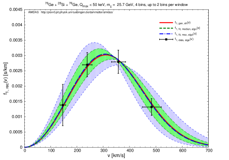
In Figs. 25 (cf. Figs. 10), the shifted Maxwellian velocity distribution with two fitting parameters and has been tested to fit to the reconstructed–input data. Only the Gaussian probability distribution for both fitting parameters with expectation values of km/s and km/s and a common 1 uncertainty of 20 km/s is considered here.
Astonishingly, with only four available data points the reconstructed velocity distribution functions could match the true (input) one very precisely: the systematic deviation of is negligible and that of is only a few km/s, the statistical uncertainties on two fitting parameters are also only and , respectively.
Variated shifted Maxwellian velocity distribution
In Figs. 26 (cf. Figs. 12), the variated shifted Maxwellian velocity distribution with two parameters and has been tested to fit to the reconstructed–input data. Only the Gaussian probability distribution for both fitting parameters with expectation values of km/s and km/s and a common 1 uncertainty of 20 km/s is considered here.
It can be seen that, although the statistical uncertainty bands are a bit wider than those given with the shifted Maxwellian distribution, with only four available data points the reconstructed velocity distribution function could also match the true (input) one very well. Moreover, as shown in Secs. 3.2.4 and 3.3.4, the second fitting parameter could also be pinned down very precisely with a negligible systematic deviation (see Table 14).
In Table 14, we give the reconstructed results with all four fitting velocity distribution functions for the input WIMP mass of GeV. Both cases with the true (input) and the reconstructed WIMP masses have been simulated and summarized.
3.4.2 For a heavy WIMP mass
(a) (b)
(a) (b)
(c) (d)
(a) (b)
(c) (d)
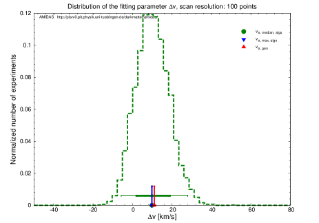
We consider now a rather heavy WIMP mass of GeV. The maximal experimental cut–off energy for both targets in our simulations demonstrated here has been set again as keV. And, as usual, the width of the first energy bin in Eq. (18) has been set as keV, five bins between and are used () and up to three bins have been combined to a window ().
Simple Maxwellian velocity distribution
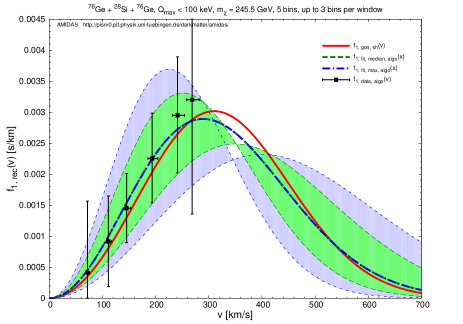
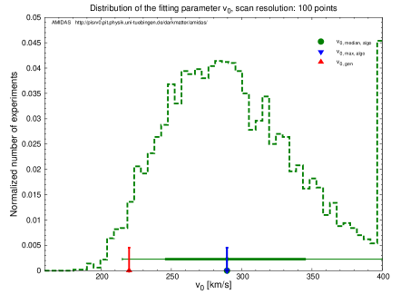
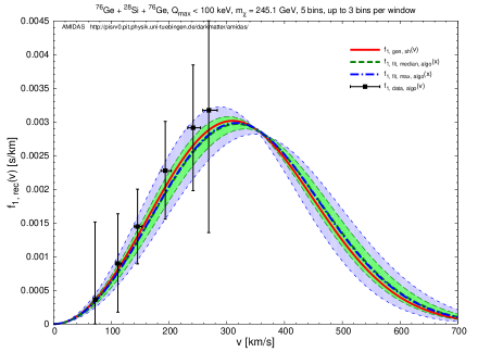
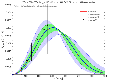
For a heavy WIMP mass, due to the (large) statistical fluctuation discussed in Ref. [6], our reconstructed velocity distribution functions given in Fig. 27(a) (cf. Figs. 5(c) and 24(a)) have clearly a (much) wider statistical uncertainty bands; the statistical uncertainties on the reconstructed Solar Galactic velocity are also (much) larger as km/s. And, as shown in Fig. 27(b), a considerable fraction of the reconstructed would excess our scanning upper bound of 400 km/s. Remind that the bin at km/s is an “overflow” bin, which contains also the experiments with the best–fit value of km/s.
Nevertheless, comparing to the much larger 1 statistical uncertainty on the reconstructed–input data (solid black vertical bars), our Bayesian reconstruction with an in fact improper fitting velocity distribution could still offer an approximation with only km/s systematic deviation of the peak of the reconstructed velocity distribution from that of the true (input) one.
Shifted Maxwellian velocity distribution
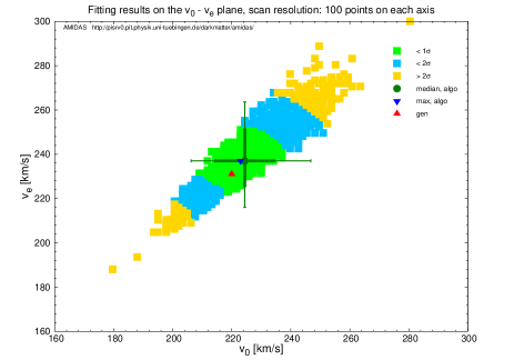
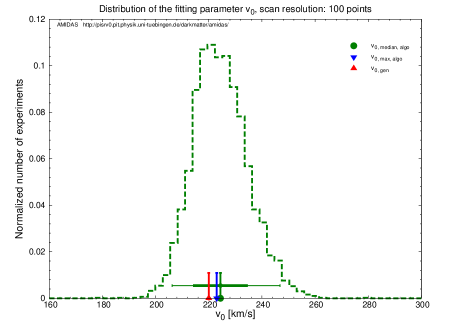
In Figs. 28 (cf. Figs. 10 and 25), the shifted Maxwellian velocity distribution with two fitting parameters and has been tested to fit to the reconstructed–input data. Only the Gaussian probability distribution for both fitting parameters with expectation values of km/s and km/s and a common 1 uncertainty of 20 km/s is considered here.
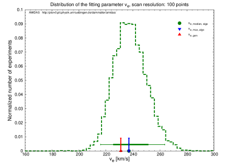
With a proper fitting velocity distribution and one more fitting parameter, the reconstructed velocity distribution could now match the true (input) one very precisely with much narrower statistical uncertainty bands. Additionally, the statistical uncertainties on the fitting parameters and can be significantly reduced to only and , respectively. Note that, as shown in Table 15, the use of the one–parameter shifted Maxwellian velocity distribution with only one fitting parameter and the fixed relation between and would give a (much) wider statistical uncertainty bands of the reconstructed velocity distribution as well as a (much) larger statistical uncertainties on the reconstructed Solar Galactic velocity: % to a factor of larger.
Variated shifted Maxwellian velocity distribution
| Input: shifted Maxwellian velocity distribution | ||||||
| Reconstruction: simple Maxwellian velocity distribution | ||||||
| Parameter | WIMP mass | Prob. dist. | Max. | Median | 1 range | 2 range |
| [km/s] | Input | Flat | 287.2 | [265.6, 316.0] | [246.4, 356.8] | |
| Gaussian | 284.8 | [268.0, 304.0] | [253.6, 320.8] | |||
| Reconst. | Flat | 289.6 | [246.4, 344.8] | [215.2, 400.0] | ||
| Gaussian | 289.6 | [256.0, 320.8] | [227.2, 352.0] | |||
| Reconstruction: one–parameter shifted Maxwellian velocity distribution | ||||||
| [km/s] | Input | Flat | 209.0 | [193.6, 227.2] | [182.4, 252.4] | |
| Gaussian | 218.8 | [209.0, 228.6] | [199.2, 238.4] | |||
| Reconst. | Flat | 211.8 | [181.0, 248.2] | [160.0, 300.0] | ||
| Gaussian | 218.8 | [202.0, 238.4] | [185.2, 256.6] | |||
| Reconstruction: shifted Maxwellian velocity distribution | ||||||
| [km/s] | Input | Gaussian | 223.0 | [216.0, 228.6] | [209.0, 235.6] | |
| Reconst. | Gaussian | 223.0 | [214.6, 234.2] | [206.2, 246.8] | ||
| [km/s] | Input | Gaussian | 237.0 | [230.0, 244.0] | [221.6, 251.0] | |
| Reconst. | Gaussian | 237.0 | [225.8, 251.0] | [216.0, 263.6] | ||
| Reconstruction: variated shifted Maxwellian velocity distribution | ||||||
| [km/s] | Input | Gaussian | 218.8 | [210.4, 228.6] | [200.6, 237.0] | |
| Reconst. | Gaussian | 220.2 | [203.4, 235.6] | [189.4, 252.4] | ||
| [km/s] | Input | Gaussian | 9.8 | [4.6, 15.0] | [, 18.9] | |
| Reconst. | Gaussian | 9.8 | [2.0, 18.9] | [, 28.0] | ||
Finally, in Figs. 29 (cf. Figs. 12 and 26), we test the possibility of improving the reconstruction precision by the use of the variated shifted Maxwellian velocity distribution with two fitting parameters and . Only the Gaussian probability distribution for both fitting parameters with expectation values of km/s and km/s and a common 1 uncertainty of 20 km/s is considered here.
While the reconstructed velocity distribution function could still match the true (input) one very precisely with however wider statistical uncertainty bands, the “best–fit” values of both parameters and (and in turn ) could again be very precisely determined with negligible systematic deviations (see Table 15).
Note that, since the heavier the WIMP mass, the smaller the transformation constant defined in Eq. (5), for an experimental maximal cut–off energy GeV, the reconstructible velocity range of our model–independent data analysis method would be much smaller than our maximal cut–off velocity (e.g. km/s for GeV and the target). Therefore, our simulations shown in this subsection demonstrate meaningfully that, our Bayesian reconstruction of the one–dimensional WIMP velocity distribution would be an important improvement for offering more and preciser information about the Galactic halo, e.g. the position of the peak of the WIMP velocity distribution, for the WIMP mass between (20) GeV and even (500) GeV.
In Table 15, we give the reconstructed results with all four fitting velocity distribution functions for the input WIMP mass of GeV. Both cases with the true (input) and the reconstructed WIMP masses have been simulated and summarized.
3.5 Background effects
(a) (b)
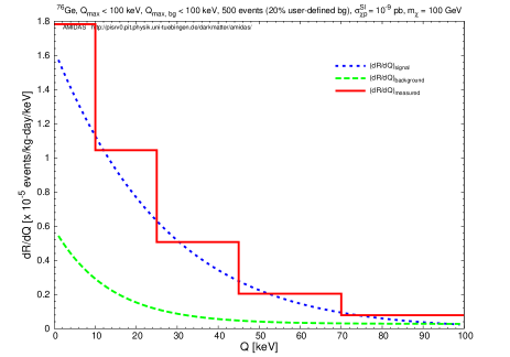
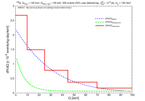
In this last part of our presentation of the numerical simulations of the Bayesian reconstruction of the WIMP velocity distribution function, we consider the effects of unrejected background events. Similar to our earlier works in Refs. [16, 15], we take into account a small fraction of artificially generated background events in the fake experimental data sets and want to study how well the WIMP velocity distribution as well as the fitting parameters could be reconstructed.
In all simulations demonstrated in this subsection, a combination of the target–dependent exponential form of the residue background spectrum introduced in Ref. [16] with a small constant component has been used:
| (48) |
where
| (49) |
and
| (50) |
Here is the recoil energy, is the atomic mass number of the target nucleus. The power index of , 0.6, is an empirical constant, which has been chosen so that the exponential background spectrum is somehow similar to, but still different from the expected recoil spectrum of the target nuclei; otherwise, there is in practice no difference between the WIMP scattering and background spectra151515 Note that, among different possible choices, we use in our simulations the atomic mass number as the simplest, unique characteristic parameter in the general analytic form (49) for defining the artificial residue background spectra for different target nuclei. However, it does not mean that the (superposition of the real) background spectra would depend simply/primarily on or on the mass of the target nucleus, . In other words, it is practically equivalent to use the expression (49) or directly for a target (cf. [23]). . Additionally, is the ratio between the exponential and constant components in the total background spectrum, which has been fixed as for all simulations.
Note that, firstly, as argued in Ref. [16], the exponential form of background spectrum is rather naive; but, since we consider here only a few tens residue background events induced by several different sources, pass all discrimination criteria, and then mix with other WIMP–induced events in our data sets of a few hundreds total events, an exact form of background spectrum for each target nucleus would not be crucial and the exponential + constant form of background spectrum in Eq. (48) should practically not be unrealistic. Secondly, as demonstrated in Refs. [5, 6] and in the previous subsections, our Bayesian reconstruction of the one–dimensional WIMP velocity distribution requires only measured recoil energies and occasionally prior knowledge about the Solar and Earth’s Galactic velocities. Hence, for applying this method to future real experimental data, prior knowledge about (different) background source(s) is not required at all.
In Figs. 30, we show the measured recoil energy spectrum (solid red histogram) for a (a) and a (b) targets with an input WIMP mass of GeV. The dotted blue curve is the elastic WIMP–nucleus scattering spectrum for generating signal events, whereas the dashed green curve shows the artificial background spectrum: the exponential background spectrum given in Eq. (49) accompanied with an extra constant component, normalized to fit to the background ratio of 20%.
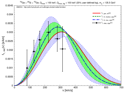
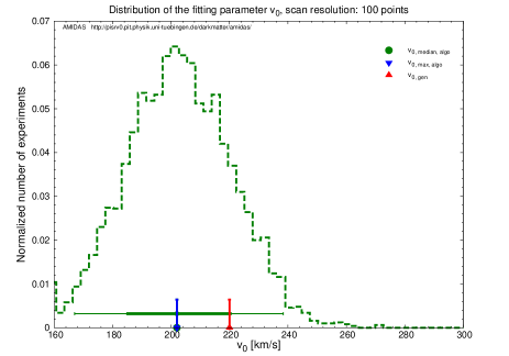
(a) (b)
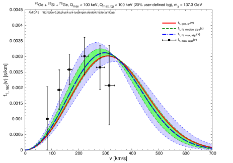
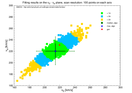
(a) (b)
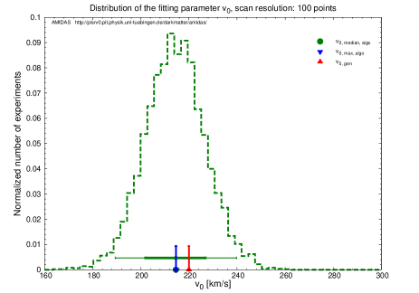
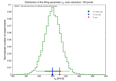
(c) (d)
3.5.1 For a moderate WIMP mass
We consider first a moderate input WIMP mass of GeV. The shifted Maxwellian velocity distribution given in Eq. (41) is used for generating WIMP signals. All input setup and fitting parameters are the same as in Sec. 3.2 (see Table 3) and a fraction of 20% background events has been taken into account. Additionally, as in Sec. 3.4, we consider only the use of the Gaussian probability distribution for the fitting parameters: and or as well as the use of the reconstructed WIMP mass.
| Input: shifted Maxwellian velocity distribution | ||||||
| Reconstruction: simple Maxwellian velocity distribution | ||||||
| Parameter | WIMP mass | Prob. dist. | Max. | Median | 1 range | 2 range |
| [km/s] | Input | Flat | 284.8 | [265.6, 308.8] | [244.0, 337.6] | |
| Gaussian | 284.8 | [268.0, 301.6] | [251.2, 320.8] | |||
| Reconst. | Flat | 253.6 | [222.4, 289.6] | [193.6, 332.8] | ||
| Gaussian | 258.4 | [232.0, 287.2] | [203.2, 316.0] | |||
| Reconstruction: one–parameter shifted Maxwellian velocity distribution | ||||||
| [km/s] | Input | Flat | 211.8 | [196.4, 228.6] | [181.0, 248.2] | |
| Gaussian | 217.4 | [207.6, 228.6] | [195.0, 239.8] | |||
| Reconst. | Flat | 188.0 | [165.6, 214.6] | [160.0, 244.0] | ||
| Gaussian | 202.0 | [185.2, 220.2] | [167.0, 238.4] | |||
| Reconstruction: shifted Maxwellian velocity distribution | ||||||
| [km/s] | Input | Gaussian | 225.8 | [217.4, 232.8] | [189.4, 239.8] | |
| Reconst. | Gaussian | 214.6 | [202.0, 226.8] | [189.4, 239.8] | ||
| [km/s] | Input | Gaussian | 231.4 | [223.0, 239.8] | [213.2, 248.2] | |
| Reconst. | Gaussian | 220.2 | [209.0, 232.8] | [196.4, 245.4] | ||
| Reconstruction: variated shifted Maxwellian velocity distribution | ||||||
| [km/s] | Input | Gaussian | 220.2 | [210.4, 228.6] | [200.6, 239.8] | |
| Reconst. | Gaussian | 204.8 | [189.4, 221.6] | [174.0, 237.0] | ||
| [km/s] | Input | Gaussian | 5.9 | [, 11.1] | [, 16.3] | |
| Reconst. | Gaussian | [, 7.2] | [, 15.0] | |||
One–parameter shifted Maxwellian velocity distribution
In Fig. 31(a), it can be seen first that, due to the extra background events in both of the low and high energy ranges (see Figs. 30), the reconstructed–input data (solid black vertical bars) would be shifted (strongly) to the low–velocity range161616 Note that, as shown in Fig. 31(a) and 32(a), the reconstructed WIMP mass is now overestimated: GeV. : the peak of the solid black crosses is now at km/s, i.e. km/s smaller then the position of the true (input) velocity distribution. However, our simulation shown in Fig. 31(a) indicates clearly and importantly that, by assuming the shifted Maxwellian WIMP velocity distribution and the time–averaged relation between the Solar and Earth’s Galactic velocities, the reconstructed WIMP velocity distributions could alleviate this systematic shift: the deviations of the peaks of the ( statistical uncertainty bands of the) reconstructed velocity distributions would only be km/s.
In fact, it has also been found that, once an (approximately) precisely determined (true) WIMP mass could be used, the reconstructed WIMP velocity distribution could match the true (input) one very precisely: the deviation of the reconstructed would be km/s (flat) or even negligible (Gaussian) (see Table 16).
Note that, although a fraction of 20% unrejected background events has been mixed (artificially) into the analyzed (pseudo–)data sets, the (1 statistical uncertainty on the) median value of the reconstructed ’s ( km/s) would still cover the true (input) Solar Galactic velocity of km/s. Moreover, once we take into account the statistical fluctuation of the reconstructed–input data (the solid black vertical bars), the effect of 20% residue background events on reconstructing information about the (shape of the) WIMP velocity distribution function would not be very significant.
Shifted Maxwellian velocity distribution
In Figs. 32, we release the fixed relation between and and determine these two parameters simultaneously and independently.
It can be seen that, firstly, the statistical uncertainty bands are obviously narrower than those shown in Fig. 31(a); the deviations of the peaks of the reconstructed velocity distributions from that of the true (input) one would be reduced to only km/s. In addition, the systematic deviations and the (1 statistical uncertainties on the) median values of the reconstructed fitting paramaters and shown in Figs. 32(c) and (d) are also (much) smaller than that shown in Fig. 31(b) (see Table 16). Note here that, as given in Table 16, once an (approximately) precisely determined (true) WIMP mass could be used, one could reconstruct the WIMP velocity distribution function very precisely with very small or even negligible systematic deviations of both two fitting parameters. This means that, our Bayesian reconstruction method for the WIMP velocity distribution function would not be affected (significantly) by a fraction of % unrejected background events mixed in the analyzed data sets (for a WIMP mass of GeV).
In Table 16, we give the reconstructed results with all four fitting velocity distribution functions for data sets mixed with 20% background events and the input WIMP mass of GeV. Both cases with the true (input) and the reconstructed WIMP masses have been simulated and summarized.
3.5.2 For a light WIMP mass
Now, we consider the case with a light input WIMP mass of GeV. Simulation setup is the same as in Sec. 3.4.1 and a fraction of 20% background events has been taken into account.
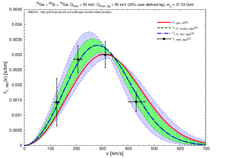
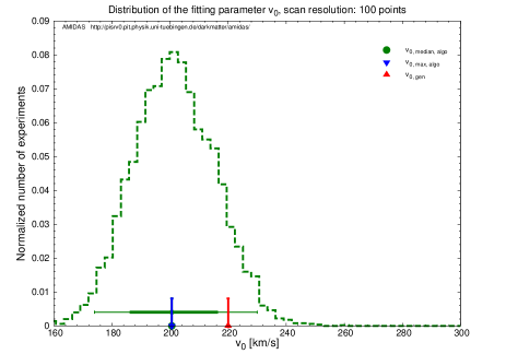
(a) (b)
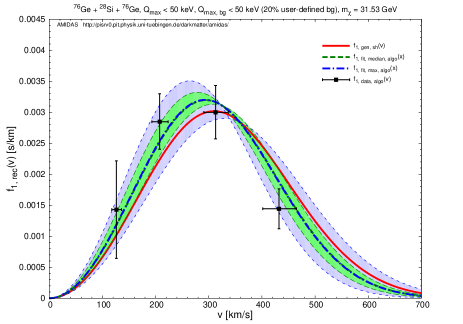
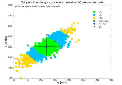
(a) (b)
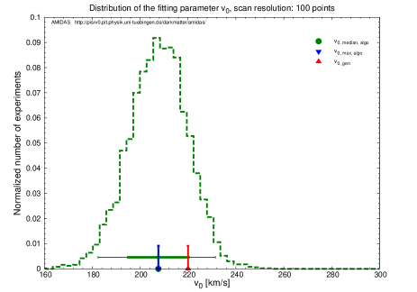
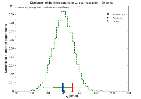
(c) (d)
One–parameter shifted Maxwellian velocity distribution
Since the reconstructed WIMP mass would be % overestimated ( GeV) due to the extra background events and only four reconstructed–input data points are available, Fig. 33(a) shows that the “best–fit” one–parameter shifted Maxwellian velocity distribution functions would match not the true (input) velocity distribution (solid red curve), but the analyzed data points (solid black crosses) well. Nevertheless, at least, the 2 statistical uncertainty band of the reconstructed velocity distributions could cover the true (input) one; the systematic deviations of the peaks of the reconstructed velocity distributions from that of the true (input) one would also only be km/s. Meanwhile, the 2 statistical uncertainty on the median value of the reconstructed ’s ( km/s) would still cover the true (input) Solar Galactic velocity of km/s. This could be further improved by using an (approximately) precisely determined (true) WIMP mass to be km/s (flat) and km/s (Gaussian) (see Table 17).
Shifted Maxwellian velocity distribution
As the case of the 100 GeV WIMP mass shown in Figs. 31(a) and 32(a), the statistical uncertainty bands reconstructed with the shifted Maxwellian velocity distribution with two independent fitting parameters and shown in Fig. 34(a) would clearly be much narrower than those reconstructed with only one parameter . Meanwhile, in contrast to other (presented) cases, our simulations with the true (input) WIMP mass show that the reconstructed–input data as well as the ( statistical uncertainty bands of the) reconstructed velocity distribution function would slightly shift to the high–velocity range.
Furthermore, comparing results given in Table 17 to those in Table 16, it has been found interesting and probably importantly that, for an (input) WIMP mass of (20) GeV, the use of our variated shifted Maxwellian velocity distribution given in Eq. (44) could offer preciser reconstruction results with (relatively) smaller statistical uncertainties, although fewer (four in our simulations) data points are available.
In Table 17, we give the reconstructed results with all four fitting velocity distribution functions for data sets mixed with 20% background events and the input WIMP mass of GeV. Both cases with the true (input) and the reconstructed WIMP masses have been simulated and summarized.
| Input: shifted Maxwellian velocity distribution | ||||||
| Reconstruction: simple Maxwellian velocity distribution | ||||||
| Parameter | WIMP mass | Prob. dist. | Max. | Median | 1 range | 2 range |
| [km/s] | Input | Flat | 308.8 | [294.4, 323.2] | [282.4, 342.4] | |
| Gaussian | 304.0 | [292.0, 316.0] | [280.0, 328.0] | |||
| Reconst. | Flat | 260.8 | [239.2, 284.8] | [220.0, 311.8] | ||
| Gaussian | 265.6 | [244.0, 284.8] | [224.8, 306.4] | |||
| Reconstruction: one–parameter shifted Maxwellian velocity distribution | ||||||
| [km/s] | Input | Flat | 228.6 | [218.8, 237.0] | [211.8, 249.6] | |
| Gaussian | 228.6 | [221.6, 235.6] | [214.6, 244.0] | |||
| Reconst. | Flat | 193.6 | [178.2, 210.4] | [164.2, 229.0] | ||
| Gaussian | 200.6 | [186.6, 216.0] | [174.0, 230.0] | |||
| Reconstruction: shifted Maxwellian velocity distribution | ||||||
| [km/s] | Input | Gaussian | 230.0 | [223.0, 237.0] | [216.0, 244.0] | |
| Reconst. | Gaussian | 207.6 | [195.0, 220.2] | [182.4, 231.4] | ||
| [km/s] | Input | Gaussian | 239.8 | [232.8, 248.2] | [224.4, 255.2] | |
| Reconst. | Gaussian | 218.8 | [207.6, 231.4] | [195.0, 244.0] | ||
| Reconstruction: variated shifted Maxwellian velocity distribution | ||||||
| [km/s] | Input | Gaussian | 228.6 | [221.6, 235.6] | [216.0, 242.6] | |
| Reconst. | Gaussian | 203.4 | [192.2, 217.4] | [181.0, 228.6] | ||
| [km/s] | Input | Gaussian | 12.4 | [5.9, 16.3] | [0.7, 21.5] | |
| Reconst. | Gaussian | 2.0 | [, 8.5] | [, 15.0] | ||
3.5.3 For a heavy WIMP mass
As the last case, we consider here a heavy input WIMP mass of GeV. Simulation setup is the same as in Sec. 3.4.2. Note however that, since the constant component of the background spectrum used in our simulations would cause a strongly overestimated WIMP mass, in particular, once WIMPs are heavy (e.g. the 250 GeV input WIMP mass would now be reconstructed as GeV) [16], the ratio of the background events in the analyzed data sets has been set as only 10% [15].
One–parameter shifted Maxwellian velocity distribution
As usual, we consider first the one–parameter shifted Maxwellian velocity distribution function to fit the reconstructed–input data points.
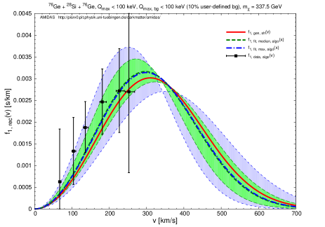
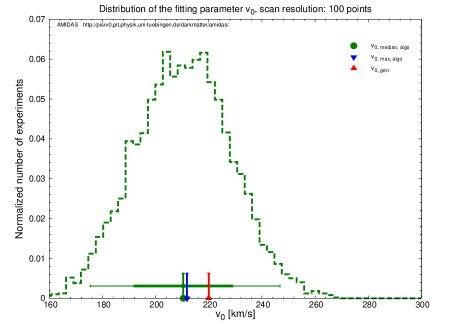
(a) (b)
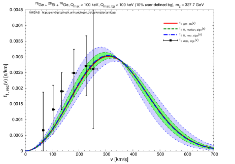
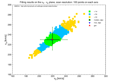
(a) (b)
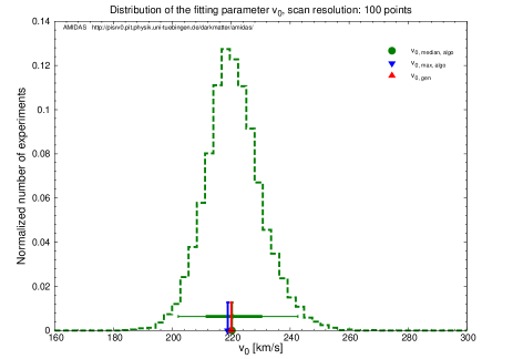
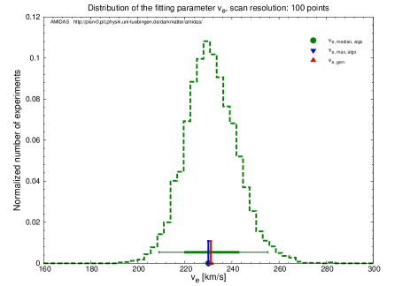
(c) (d)
In Figs. 35, we can see unexpectedly that, although the input WIMP mass is pretty heavy, the systematic deviations of the peak positions of the reconstructed WIMP velocity distribution functions from that of the true (input) one would be only km/s (for 10% background ratio!). This might be due to that, as shown in Sec. 3.4.2, for our used experimental maximal cut–off energy GeV and the target, the reconstructible velocity range would only be km/s (shifted slightly to the low–velocity range due to the overestimated WIMP mass) and thus this maximal reconstructible velocity is theoretically smaller than the position of the peak of the velocity distribution function (see e.g. Fig. 35(a)). This means that the approximately monotonically increased shape of the reconstructed–input data points (solid black vertical bars) with pretty large 1 statistical uncertainties would alleviate the effects of the overestimations of the analyzed (reconstructed–input) data points and the reconstructed WIMP mass caused by the extra background events.
| Input: shifted Maxwellian velocity distribution | ||||||
| Reconstruction: simple Maxwellian velocity distribution | ||||||
| Parameter | WIMP mass | Prob. dist. | Max. | Median | 1 range | 2 range |
| [km/s] | Input | Flat | 277.6 | [256.0, 304.0] | [239.2, 342.4] | |
| Gaussian | 277.6 | [260.8, 296.8] | [246.4, 316.0] | |||
| Reconst. | Flat | 263.2 | [224.8, 311.2] | [200.8, 378.4] | ||
| Gaussian | 268.0 | [236.8, 301.6] | [212.8, 335.2] | |||
| Reconstruction: one–parameter shifted Maxwellian velocity distribution | ||||||
| [km/s] | Input | Flat | 203.4 | [189.4, 222.6] | [175.4, 248.2] | |
| Gaussian | 216.0 | [204.8, 225.8] | [195.0, 235.6] | |||
| Reconst. | Flat | 195.0 | [165.6, 227.2] | [160.0, 272.0] | ||
| Gaussian | 211.8 | [192.2, 228.6] | [175.4, 246.8] | |||
| Reconstruction: shifted Maxwellian velocity distribution | ||||||
| [km/s] | Input | Gaussian | 221.6 | [214.6, 228.6] | [207.6, 235.6] | |
| Reconst. | Gaussian | 218.8 | [211.8, 230.0] | [202.0, 242.6] | ||
| [km/s] | Input | Gaussian | 232.8 | [225.8, 241.2] | [217.4, 248.2] | |
| Reconst. | Gaussian | 230.0 | [220.2, 242.6] | [209.0, 255.2] | ||
| Reconstruction: variated shifted Maxwellian velocity distribution | ||||||
| [km/s] | Input | Gaussian | 216.0 | [207.6, 225.8] | [197.8, 235.6] | |
| Reconst. | Gaussian | 210.4 | [196.4, 228.6] | [181.0, 245.4] | ||
| [km/s] | Input | Gaussian | 7.2 | [2.0, 12.4] | [, 17.6] | |
| Reconst. | Gaussian | 4.6 | [, 12.4] | [, 21.5] | ||
Shifted Maxwellian velocity distribution
Now we use the shifted Maxwellian velocity distribution function with two independent fitting parameters and to fit the reconstructed–input data points. Astonishingly and unexpectedly (probably accidentally), Figs. 36 show that both of the “best–fit” results of the parameters and are almost exact as the true (input) values and the 1 statistical uncertainties on and are only km/s.
Meanwhile, in contrast to our simulation results with the variated shifted Maxwellian velocity distribution function shown previously, for the case of the 250 GeV WIMP mass with 10% background ratio, the Bayesian reconstructed parameter could have a (much) larger deviations from the true (estimated) value (see Table 18)!
In Table 18, we give the reconstructed results with all four fitting velocity distribution functions for data sets mixed with 10% background events and the input WIMP mass of GeV. Both cases with the true (input) and the reconstructed WIMP masses have been simulated and summarized.
4 Summary and conclusions
In this paper, we extended our earlier work on the development of the model–independent data analysis method for the reconstruction of the (time–averaged) one–dimensional velocity distribution of Galactic WIMPs and introduced the Bayesian fitting procedure of the theoretical velocity distribution functions.
In this fitting procedure, the (rough) velocity distribution reconstructed by using raw experimental data, i.e. measured recoil energies, with one or more different target nuclei has been used as reconstructed–input data (points). By assuming a fitting WIMP velocity distribution function and scanning the parameter space based on the Bayesian analysis, the (fitting) astronomical characteristic parameters, e.g. the Solar and Earth’s Galactic velocities and , would be pinned down as the output results and thus the functional form of the one–dimensional velocity distribution can be reconstructed (instead of only a few discrete points).
As the first test of our Bayesian reconstruction method for the one–dimensional WIMP velocity distribution function, we used the simplest isothermal spherical Galactic halo model for both generating WIMP–signal events and as the assumed velocity distribution with the unique fitting parameter: the Solar Galactic velocity . Our simulations show that, with (only) 500 recorded events (on average) and without prior knowledge about the Solar Galactic velocity, could in principle be pinned down with a negligible deviation and a 1 statistical uncertainty of only km/s (with a precisely known WIMP mass) or km/s (with a reconstructed WIMP mass), respectively. Moreover, once (rough) information about the Solar Galactic velocity can be given, the statistical uncertainties on the reconstructed could even be reduced to %.
For more realistic consideration, we then took into account the orbital motion of the Solar system around our Galaxy as well as that of the Earth around the Sun and turned to use the shifted Maxwellian velocity distribution function for generating WIMP signals. As comparisons, four different fitting functions have been considered: the simple and the (one–parameter and variated) shifted Maxwellian velocity distributions. It has been found that, firstly, with an improper assumed fitting function (e.g. the simple Maxwellian velocity distribution here), the WIMP velocity distribution could still be reconstructed and offer some important information about Galactic WIMPs, e.g. the rough position of the peak of the one–dimensional velocity distribution function. The deviations of the peaks of the reconstructed velocity distributions from that of the true (input) one would be only km/s. However, the best–fit value(s) of the fitting parameter(s) would be unexpected/unreasonable. For instance, the reconstructed Solar Galactic velocity would be 2 (with the reconstructed WIMP mass) or even 4 (with the input WIMP mass) apart from its theoretical estimate. Such an observation could in turn be an important criterion on the assumption of fitting velocity distribution function.
Moreover, our simulations with the (one–parameter and variated) shifted Maxwellian velocity distributions show that, although in all of these three cases the reconstructed velocity distributions could match the true (input) one pretty precisely, with two fitting parameters the statistical uncertainty bands of the reconstructed velocity distributions would be narrower then those with only one fitting parameter. In addition, the use of the variation of the shifted Maxwellian velocity distribution could (strongly) reduce the systematic deviations of the determinations of the characteristic Solar and Earth’s Galactic velocities and , with however a bit larger statistical uncertainties.
Furthermore, we considered also a modification of the simple Maxwellian velocity distribution with an extra power index as the generating WIMP velocity distribution. First, we used the simple Maxwellian velocity distribution without the power index as the test fitting function. Since the difference between the modification and the original simple Maxwellian velocity distributions are very tiny, the reconstructed velocity distribution function could match the true (input) one very precisely and the characteristic Solar Galactic velocity could also be reconstructed with negligible systematic deviation.
Meanwhile, our simulations with the (one–parameter and variated) shifted Maxwellian velocity distribution functions show that, although the positions of the peak of the reconstructed velocity distribution would be only km/s deviated from the true (input) one, a clear 2 to even 6 difference between the best–fit values of the Solar and/or the Earth’s Galactic velocities and the true (input) ones could be observed. Such results would in turn indicate evidently the improper assumption of the shifted Maxwellian velocity distribution function.
Moreover, from the simulations with the modified simple Maxwellian velocity distribution with the power index as the second fitting parameter, it has been found that our Bayesian reconstruction of the WIMP velocity distribution would be (totally) non–sensitive on the power index. This means that, unfortunately, with only a few hundreds of recorded WIMP events it would still be impossible to distinguish (evidently) different subtle variations of the (simple and shifted) WIMP velocity distribution functions.
As comparisons, we considered also a light and a heavy input WIMP masses. For the case of light WIMPs, due to the sharp shapes of the recoil energy spectra and the small kinetic maximal cut–off energies, the recorded WIMP events would need to be separated into fewer bins/windows. However, our simulations show that, with only four available reconstructed–input data points, the true (input) velocity distribution function could astonishingly be reconstructed very precisely. On the other hand, once WIMPs are heavy, the statistical fluctuation on the reconstructed WIMP mass becomes pretty large and hence the Bayesian reconstructions of the velocity distribution as well as of the Solar and Earth’s Galactic velocities would have large statistical uncertainties. Nevertheless, the reconstructed velocity distribution function with the best–fit characteristic Solar and Earth’s Galactic velocities could still match the true (input) one very precisely.
Finally, the effects of residue (unrejected) background events mixed in data sets to analyze have also been considered. Three different WIMP masses with background ratios of 10% or 20% have been tested. Although, due to the choice of our artificial residue background spectrum, the reconstructed WIMP masses would be overestimated and the (rough shape of) the reconstructed–input data points would thus be shifted (significantly) to lower velocities, the functional forms of the chosen fitting velocity distributions could somehow alleviate these systematic shifts and the statistical uncertainty bands could still cover the true (input) velocity distribution. In particular, for heavy WIMPs, since the reconstructed–input data points should be in the velocity range smaller than the position of the peak of the velocity distribution function, its approximately monotonically increased shape with pretty large 1 statistical uncertainties would alleviate the effects of the overestimations of the analyzed (reconstructed–input) data points and the reconstructed WIMP mass caused by the extra background events. The reconstructed velocity distribution function could then match the true (input) one pretty well.
It would be worth to emphasize that, first, comparing to the pretty large (1) statistical uncertainties on the reconstructed–input data points (offered by our model–independent method developed in Ref. [5] with raw experimental measured recoil energies), our Bayesian reconstruction of the WIMP velocity distribution function introduced here with only a few km/s deviation and (10) km/s 1 statistical uncertainties on the reconstructed Solar and Earth’s Galactic velocities would be a remarkable improvement.
Second, all our simulations show importantly that, even initial values different slightly from the true (input) setup have been used as the expectation values for the Gaussian probability distribution of the fitting parameters, these fitting parameters could still be pinned down (pretty) precisely. As long as a proper assumed fitting velocity distribution function is used, the best–fit values of the reconstructed parameters could always be less than 1 apart from the true (input/theoretical) values. This observation indicates that rough, slightly incorrect prior knowledge about our fitting parameters would not affect (significantly) the reconstructed results in our Bayesian reconstruction procedure.
Moreover, by rewriting the functional form of the (basic) fitting velocity distribution function, one could not only pin down the fitting parameters more precisely, but also occasionally reduce the statistical uncertainties on the reconstructed parameters.
In summary, we developed in this paper the Bayesian reconstruction procedure for fitting theoretically predicted models of the one–dimensional WIMP velocity distribution function to data (points), which can be reconstructed directly from experimental measured recoil energies. Hopefully, this extension of our earlier work could offer more useful information about the Dark Matter halo, which could further be used in e.g. indirect DM detection experiments.
Acknowledgments
The author appreciates Mei-Yu Wang for useful discussions about models of the velocity distribution of Galactic WIMPs. The author would also like to thank the Physikalisches Institut der Universität Tübingen for the technical support of the computational work presented in this paper as well as the friendly hospitality of the Graduate School of Science and Engineering for Research, University of Toyama, the Institute of Modern Physics, Chinese Academy of Sciences, the Center for High Energy Physics, Peking University, and the Xinjiang Astronomical Observatory, Chinese Academy of Sciences, where part of this work was completed. This work was partially supported by the National Science Council of R.O.C. under the contracts no. NSC-98-2811-M-006-044 and no. NSC-99-2811-M-006-031 as well as the CAS Fellowship for Taiwan Youth Visiting Scholars under the grant no. 2013TW2JA0002.
Appendix A Formulae needed in Sec. 2.1
Here we list all formulae needed for the model–independent method for the reconstruction of the one–dimensional WIMP velocity distribution function described in Sec. 2.1. Detailed derivations and discussions can be found in Ref. [5].
First, by using the standard Gaussian error propagation, the expression for the uncertainty on the logarithmic slope can be given from Eq. (11) directly as
| (A1) |
with
| (A2) |
For replacing the “bin” quantities by “window” quantities, one needs the covariance matrix for , which follows directly from the definition (23):
| (A3) | |||||
Note that, firstly, has been assumed here and the covariance matrix is, of course, symmetric. Secondly, the sum is understood to vanish if the two windows , do not overlap, i.e. if . Moreover, from Eq. (24), we can get
| (A4) |
where has again been taken. And the mixed covariance matrix can be given by
| (A5) |
Note here that this sub–matrix is not symmetric under the exchange of and . In the definition of and we therefore have to distinguish two cases:
| (A8) |
As before, the sum in Eq. (A5) is understood to vanish if .
References
- [1] G. Jungman, M. Kamionkowski and K. Griest, “Supersymmetric Dark Matter”, Phys. Rep. 267, 195–373 (1996), arXiv:hep-ph/9506380.
- [2] M. Drees and G. Gerbier, “Mini–Review of Dark Matter: 2012”, updated minireview for “The Review of Particle Physics 2012”, arXiv:1204.2373 [hep-ph] (2012).
- [3] T. Saab, “An Introduction to Dark Matter Direct Detection Searches and Techniques”, arXiv:1203.2566 [physics.ins-det] (2012).
- [4] L. Baudis, “Direct Dark Matter Detection: the Next Decade”, Issue on “The Next Decade in Dark Matter and Dark Energy”, Phys. Dark Univ. 1, 94–108 (2012), arXiv:1211.7222 [astro-ph.IM].
- [5] M. Drees and C.-L. Shan, “Reconstructing the Velocity Distribution of Weakly Interacting Massive Particles from Direct Dark Matter Detection Data”, J. Cosmol. Astropart. Phys. 0706, 011 (2007), arXiv:astro-ph/0703651.
- [6] M. Drees and C.-L. Shan, “Model–Independent Determination of the WIMP Mass from Direct Dark Matter Detection Data”, J. Cosmol. Astropart. Phys. 0806, 012 (2008), arXiv:0803.4477 [hep-ph].
- [7] B. J. Barlow, “Statistics: A Guide to the Use of Statistical Methods in the Physical Sciences”, Wiley (1993).
- [8] G. D’Agostini, “Probability and Measurement Uncertainty in Physics: A Bayesian Primer”, arXiv:hep-ph/9512295 (1995).
- [9] Y. Akrami, C. Savage, P. Scott, J. Conrad and J. Edsjö, “Statistical Coverage for Supersymmetric Parameter Estimation: A Case Study with Direct Detection of Dark Matter”, J. Cosmol. Astropart. Phys. 1107, 002 (2011), arXiv:1011.4297 [hep-ph]; “How Well Will Ton–Scale Dark Matter Direct Detection Experiments Constrain Minimal Supersymmetrh?”, J. Cosmol. Astropart. Phys. 1104, 012 (2011), arXiv:1011.4318 [astro-ph.CO].
-
[10]
M. Pato, L. Baudis, G. Bertone, R. Ruiz de Austri, L. E. Strigari and R. Trotta,
“Complementarity of Dark Matter Direct Detection Targets”,
Phys. Rev. D 83, 083505 (2011),
arXiv:1012.3458 [astro-ph.CO];
M. Pato, “What Can(not) be Measured with Ton–Scale Dark Matter Direct Detection Experiments”, J. Cosmol. Astropart. Phys. 1110, 035 (2011), arXiv:1106.0743 [astro-ph.CO];
M. Pato, L. E. Strigari, R. Trotta and G. Bertone, “Taming Astrophysical Bias in Direct Dark Matter Searches”, J. Cosmol. Astropart. Phys. 1302, 041 (2013), arXiv:1211.7063 [astro-ph.CO]. -
[11]
C. Arina, J. Hamann and Y. Y. Y. Wong,
“A Bayesian View of the Current Status of Dark Matter Direct Searches”,
J. Cosmol. Astropart. Phys. 1109, 022 (2011),
arXiv:1105.5121 [hep-ph];
C. Arina, J. Hamann, R. Trotta and Y. Y. Y. Wong, “Evidence for Dark Matter Modulation in CoGeNT”, J. Cosmol. Astropart. Phys. 1203, 008 (2011), arXiv:1111.3238 [hep-ph];
C. Arina, “Chasing a Consistent Picture for Dark Matter Direct Searches”, Phys. Rev. D 86, 123527 (2012), arXiv:1210.4011 [hep-ph]; “Bayesian Analysis of Multiple Direct Detection Experiments”, arXiv:1310.5718 [hep-ph] (2013). - [12] C. Strege, R. Trotta, G. Bertone, A. H. G. Peter and P. Scott, “Fundamental Statistical Limitations of Future Dark Matter Direct Detection Experiments”, Phys. Rev. D 86, 023507 (2012), arXiv:1201.3631 [hep-ph].
- [13] D. G. Cerdeo et al., “Complementarity of Dark Matter Direct Detection: the Role of Bolometric Targets”, J. Cosmol. Astropart. Phys. 1307, 028 (2013), arXiv:1304.1758 [hep-ph].
- [14] B. J. Kavanagh, “Parametrizing the Local Dark Matter Speed Distribution: A Detailed Analysis”, Phys. Rev. D 89, 085026 (2014), arXiv:1312.1852 [astro-ph.CO].
- [15] C.-L. Shan, “Effects of Residue Background Events in Direct Dark Matter Detection Experiments on the Reconstruction of the Velocity Distribution Function of Halo WIMPs”, J. Cosmol. Astropart. Phys. 1006, 029 (2010), arXiv:1003.5283 [astro-ph.HE].
- [16] Y.-T. Chou and C.-L. Shan, “Effects of Residue Background Events in Direct Dark Matter Detection Experiments on the Determination of the WIMP Mass”, J. Cosmol. Astropart. Phys. 1008, 014 (2010), arXiv:1003.5277 [hep-ph].
-
[17]
K. Freese, J. Frieman and A. Gould,
“Signal Modulation in Cold-Dark-Matter Detection”,
Phys. Rev. D 37, 3388–-3405 (1988);
K. Freese, M. Lisanti and C. Savage, “Annual Modulation of Dark Matter: A Review”, Rev. Mod. Phys. 85, 1561–1581 (2013), arXiv:1209.3339 [astro-ph.CO]. - [18] M. Lisanti, L. E. Strigari, J. G. Wacker and R. H. Wechsler, “The Dark Matter at the End of the Galaxy”, Phys. Rev. D 83, 023519 (2011), arXiv:1010.4300 [astro-ph.CO].
-
[19]
Y.-Y. Mao, L. E. Strigari, R. H. Wechsler, H.-Y. Wu and O. Hahn,
“Halo–to–Halo Similarity and Scatter in the Velocity Distribution of Dark Matter”
Astrophys. J. 764, 35 (2013),
arXiv:1210.2721 [astro-ph.CO];
Y.-Y. Mao, L. E. Strigari and R. H. Wechsler, “Connecting Direct Dark Matter Detection Experiments to Cosmologically Motivated Halo Models”, Phys. Rev. D 89, 063513 (2014), arXiv:1304.6401 [astro-ph.CO]. - [20] M. Kuhlen, A. Pillepich, J. Guedes and P. Madau, “The Distribution of Dark Matter in the Milky Way’s Disk”, Astrophys. J. 784, 161 (2014), arXiv:1308.1703 [astro-ph.GA].
-
[21]
C.-L. Shan,
the AMIDAS (A Model–Independent Data Analysis System)
package and website for direct Dark Matter detection experiments and phenomenology,
http://pisrv0.pit.physik.uni-tuebingen.de/darkmatter/amidas/ (2009);
the mirror website on TiResearch (Taiwan interactive Research),
http://www.tir.tw/phys/hep/dm/amidas/. - [22] C.-L. Shan, “AMIDAS-II: Upgrade of the AMIDAS Package and Website for Direct Dark Matter Detection Experiments and Phenomenology”, arXiv:1403.5611 [astro-ph.IM] (2014).
- [23] A. M. Green, “Determining the WIMP Mass from a Single Direct Detection Experiment, a More Detailed Study”, J. Cosmol. Astropart. Phys. 0807, 005 (2008), arXiv:0805.1704 [hep-ph].