Decay constants of the pion and its excitations on the lattice.

Abstract

We present a calculation using lattice QCD of the ratios of decay constants of the excited states of the pion, to that of the pion ground state, at three values of the pion mass between 400 and 700 MeV, using an anisotropic clover fermion action with three flavors of quarks. We find that the decay constant of the first excitation, and more notably of the second, is suppressed with respect to that of the ground-state pion, but that the suppression shows little dependence on the quark mass. The strong suppression of the decay constant of the second excited state is consistent with its interpretation as a predominantly hybrid state.

I Introduction

Obtaining precise information about excited hadrons poses numerous challenges. The principal computational challenge arises from the faster decay of their Euclidean correlation functions in comparison with those of the ground state, which leads to the worsening of the signal-to-noise ratio. Additional complications arise in constructing hadronic operators, where we seek to balance the computational cost with the level of overlap achieved by a set of operators.

Despite these obstacles, advances in computational lattice QCD techniques are such that precise quantitative calculations that can confront both existing and forthcoming experiments are increasingly feasible. Experiments include those at the 12 GeV upgrade of the Continuous Electron Beam Accelerator Facility (CEBAF) at Jefferson Lab Dudek:2012vr , with its new meson spectroscopy program in the mass range up to 3.5 GeV. The expectation is that new data produced in such experiments, combined with recent lattice QCD results aimed at extracting the spectrum of the excited states for both mesons and baryons Dudek:2009qf ; Dudek:2010wm ; Dudek:2011pd ; Dudek:2011tt ; Dudek:2012rd , will represent a unique opportunity for the study of the nature of confinement mechanism, and for identifying the role of gluonic degrees of freedom in the spectrum.

The theoretical work presented here is devoted to the study of some of the properties of excited states. It represents the first step in a program to investigate quark distribution amplitudes, which can be extracted from the vacuum-to-hadron matrix elements of quark bilinear operators in the case of mesons, and of three-quark operators in the case of baryons. These amplitudes can be used to provide predictions for form factors and transition form factors at high momentum transfers; in the case of baryons, the study of transition form factors at high $Q^{2}$ is a focus of the JLab CLAS12 experiment, with the aim of exploring the transition from hadronic to quark-and-gluon-dominated dynamics.

In this paper, we provide details of a calculation of the leptonic decay constant of the pion - the lightest system with a valence quark-antiquark structure - and its excitations. A knowledge of the decay constants of the excited states, as well as of the ground state, is important in delineating between different QCD-inspired pictures of the meson spectrum, as well as demonstrating the feasibility of studying the properties of highly excited states within lattice QCD.

The layout of the remainder of the paper is as follows. In the next section, we outline briefly the significance of the pseudoscalar decay constants, and the state of our understanding for the pion. We then describe our computational methodology for extracting the decay constants not only of the ground-state pion, but of its excitations, and provide details of the lattices used in our calculation. In Section IV we present our results, and compare to expectations from models, and from previous lattice studies. A summary and conclusions are given in Section V, while details of some derivations are provided in Appendix.

II Pseudoscalar leptonic decay constants

Charged mesons are allowed to decay, through quark-antiquark annihilations via a virtual $W$ boson, to a charged lepton and (anti-)neutrino. The decay width for any pseudo-scalar meson $P$ of a quark content $q_{1}\bar{q}_{2}$ with mass $m_{P}$ is given by

$$\Gamma(P\to l\nu)=\frac{G_{f}^{2}}{8\pi}f_{P}^{2}m_{l}^{2}m_{P}\left(1-\frac{m_{l}^{2}}{m_{P}^{2}}\right)|V_{q_{1}\bar{q}_{2}}|^{2}.$$ (1)

Here $m_{l}$ is the mass of the lepton $l$, $G_{F}$ is the Fermi coupling constant, $V_{q_{1}\bar{q}_{2}}$ is the Cabibbo-Kobayashi-Moskawa (CKM) matrix element between the constituent quarks in $P$, and $f_{P}$ is the decay constant related to the wave-function overlap of the quark and antiquark. A charged pion can decay as $\pi\to l\nu$ (we assume here $\pi^{+}\to l^{+}\nu_{l}$ or $\pi^{-}\to l^{-}\bar{\nu}_{l}$), and its decay constant $f_{\pi}$, which dictates the strength of these leptonic pion decays, has a significance in many areas of modern physics. Thus a knowledge of $f_{\pi}$ is important for the extraction of certain CKM matrix elements, where the leptonic decay width $\Gamma$ in Eqn. (1) is proportional to $f_{P}|V_{q_{1}\bar{q}_{2}}|$. The pion decay constant, through its rôle in determining the strength of $\pi\pi$ interactions, also serves as an expansion parameter in Chiral Perturbation Theory Weinberg:1979 ; Gasser:1984 . As $|V_{ud}|$ has been quite accurately measured in super-allowed $\beta$-decays, measurements of $\Gamma(\pi^{+}\to\mu^{+}\nu)$ yield a value of $f_{\pi}$. According to PDG Beringer:2012pdg , the most precise value of $f_{\pi}$ is

$$f_{\pi^{-}}=(130.41\pm 0.03\pm 0.20)\,\,{\rm MeV}.$$ (2)

Lattice QCD enables ab initio computations of the mass spectrum and decay constants of pseudo-scalar mesons, and the calculation of the decay constant for ground-state mesons has been an important endeavor in lattice calculations for the reasons cited above. Recent lattice predictions Follana:2008prl ; Durr:2010hr ; Bazavov:2010hj ; Dowdall:2013rya for the ratio $f_{K}/f_{\pi}$ of $K^{-}$ and $\pi^{-}$ decay constants were used in order to find a value for $|V_{us}|/|V_{ud}|$ which, together with the precisely measured $|V_{ud}|$, provides an independent measure of $|V_{us}|$.

The leptonic decay constant has a further role in hadronic physics in representing the wave function at the origin, and therefore a knowledge of the decay constant not only of the lowest-lying state but of some of the excitations is important in confronting QCD-inspired descriptions of the meson spectrum. The pion excited states decay predominantly through strong decays, and therefore experimental data on their decay constants are lacking. A study based on Schwinger-Dyson equations Holl:2004fr predicted significant suppression of the excited-state pion decay constant in comparison to that of the ground state. Similar predictions, based on the QCD-inspired models and sum rules, also propose remarkably small values for the decay constant of the first pion excitation $f_{\pi_{1}}$; e.g., Volkov:1996br proposed the ratio $\frac{f_{\pi_{1}}}{f_{\pi_{0}}}$ to be of the order of one percent. The authors of Ref. Chang:2011vu in their review of meson note that the prediction in the chiral limit

$$f_{\pi_{N}}\equiv 0,N\geq 0$$

is perhaps surprising, even though some some suppression of the leptonic decay constants might be expected; for $S$-wave states, the decay constant is proportional to the wave function at the origin, and for excited states the configuration-space wave function is broader. The only lattice study of the decay constants of the excited state of the pion is that of the UKQCD Collaboration McNeile:2006qy , where they obtained $f_{\pi_{1}}/f_{\pi_{0}}=0.078(93)$ in the chiral limit, using an improved axial-vector current. We will discuss these results in further detail later.

III Computational Method

The procedure for extracting energies and hadron-to-vacuum matrix elements from a lattice calculation is to evaluate numerically Euclidean correlation functions of operators $\mathcal{O}_{i}$ and $\mathcal{O}_{j}$ of given quantum numbers, which are then expressed through their spectral representation

$$C_{ij}(t,0)=\frac{1}{V_{3}}\sum_{\vec{x},\vec{y}}\langle\mathcal{O}_{i}(\vec{x},t)\mathcal{O}^{\dagger}_{j}(\vec{y},0)\rangle=\sum_{N}\frac{Z_{i}^{N*}Z_{j}^{N}}{2E_{N}}e^{-E_{N}t}.$$ (3)

Here $Z_{N}$ is the overlap of the $N^{\rm th}$ state in the spectrum, $\pi_{N}$,

$$Z_{i}^{N}\equiv\langle\pi_{N}\mid{\cal O}^{\dagger}_{i}(0)\mid 0\rangle,$$ (4)

$E_{N}$ is the energy of the state, and $V_{3}$ is the spatial volume. The ability to perform the time-sliced sum at both source and sink is a major benefit of the “distillation” method used in our calculation.

The representation in Eqn. (3) exposes some of the challenges in the study of hadronic excitations. The contributions of the excited states are suppressed exponentially, and the extraction of subleading exponentials is a demanding problem. As we climb up the spectrum, the signal-to-noise ratio tends to worsen with increasing $t$ (correlation functions decrease rapidly while statistical noise does not), and obtaining signals from the higher excitations becomes more and more problematic. Our means of overcoming these challenges is dependent on three novel elements. Firstly, the use of anisotropic lattices with a finer temporal than spatial resolution enabling the time-sliced correlators to be examined at small Euclidean times. Secondly, the use of the variational method Michael:1985 ; Luscher:1990ck ; Blossier:2009kd with a large basis of operators derived from a continuum construction yet which satisfy the symmetries of the lattice. Finally, an efficient means of computing the necessary correlation functions through the use of “distillation” Peardon:2009gh .

III.1 Gauge Configurations

We employ the $N_{f}=2\oplus 1$ anisotropic lattices generated by the Hadron Spectrum collaboration, with two mass-degenerate light quarks of mass $m_{l}$ and a strange quark of mass $m_{s}$. The lattices employ improved gluon and “clover” fermion actions, with stout smearing restricted to the spatial directions. Details are contained in Refs. Edwards:2008ja and Lin:2009rd . Here we employ $16^{3}\times 128$ lattices having a spatial lattice spacing of $a_{s}\simeq 0.123~{}{\rm fm}$, and a renormalized anisotropy, the ratio of the spatial and temporal lattice spacings, of $\xi\simeq 3.5$. The calculations are performed at three values of the light-quark masses, corresponding to pion masses of 391, 524 and 702 MeV. The 702 MeV pion mass corresponds to the $SU(3)$-flavor-symmetric point. The parameters of the lattices used here are shown in Table 1. The mass of the $\Omega$-baryon is used to set the scale, and was determined within an estimated uncertainty of 2% in Ref. Bulava:2010yg on the same ensembles; to facilitate comparison with other calculations, we also provide the value of the Sommer parameter $r_{0}$ on each ensemble.

$N_{s}$	$N_{t}$	$a_{t}m_{l}$	$a_{t}m_{s}$	$a_{t}m_{\pi}$	$r_{0}/a_{s}$	$N_{\rm cfg}$
16	128	-0.0743	-0.0743	0.1483(2)	3.21(1)	535
16	128	-0.0808	-0.0743	0.0996(6)	3.51(1)	470
16	128	-0.0840	-0.0743	0.0691(6)	3.65(1)	480

Table 1: Lattice extents ($N_{s}$ and $N_{t}$), the bare masses of light quark $a_{t}m_{l}$ and strange quark $a_{t}m_{s}$, the pion mass $a_{t}m_{\pi}$, the Sommer scale $r_{0}$, and the number $N_{\rm cfg}$ of gauge-field configurations. On each configuration, solution vectors are computed from $N_{\rm vecs}=64$ distillation vectors Peardon:2009gh , located on a single time slice.

III.2 Variational method

A detailed description of the Hadron Spectrum Collaboration implementation of the variational method can be found in Ref. Dudek:2010wm , but we summarize it briefly here. The approach involves the solution of the generalized eigenvalue equation

$$C(t)v^{(N)}(t,t_{0})=\lambda_{N}(t,t_{0})C(t_{0})v^{(N)}(t,t_{0}).$$ (5)

At sufficiently large $t>t_{0}$, the ordered eigenvalues satisfy

$$\lambda_{N}(t,t_{0})\longrightarrow e^{-E_{N}(t-t_{0})},$$

where $E_{N}$ is the energy of the $N^{\rm th}$ state. The eigenvalues are normalized to unity at $t=t_{0}$, whilst the eigenvectors satisfy the orthogonality condition:

$$v^{(N^{\prime})\dagger}C(t_{0})v^{(N)}=\delta_{N,N^{\prime}}.$$ (6)

Identifying the energy of the $N^{\rm th}$ state with its mass, the overlap factors $Z_{i}^{N}$ of the spectral representation are straightforwardly related to the eigenvectors through

$$Z_{i}^{N}=\sqrt{2m_{N}}e^{m_{N}t_{0}/2}v_{j}^{(N)*}C_{ji}(t_{0}).$$ (7)

We can define an “ideal” operator

$$\Omega_{N}=\sqrt{2m_{N}}e^{-m_{N}t_{0}/2}v_{i}^{(N)}{\cal O}_{i}$$ (8)

within the operator space for the state $N$ Dudek:2009kk , where the $v$’s are obtained from the solution of the generalized eigenvalue equation at some $t=t_{\rm ref}$, and the operators are normalized so as to remove the dependence on $t_{0}$.

III.3 Interpolating operator basis

The efficacy of the variational method relies on an operator basis that faithfully spans the low-lying spectrum. The construction of single-particle elements of such a basis is described in detail in Refs. Dudek:2009qf and Dudek:2010wm . Briefly, each operator is constructed from elements of the general form

$$\bar{\psi}\Gamma\overleftrightarrow{D}_{i}\overleftrightarrow{D}_{j}\,...\psi,$$ (9)

where $\overleftrightarrow{D}\equiv\overleftarrow{D}-\overrightarrow{D}$ is a discretization of gauge-covariant derivatives, and $\Gamma$ is one of the sixteen Dirac matrices. We then form an operator of definite $J$ and $M$, which we denote by

$$\mathcal{O}^{J,M}=\left(\Gamma\times D_{J_{D}}^{[N]}\right)^{J}.$$ (10)

We note that both charge conjugation, for neutral particles, and parity are good symmetries on the lattice, but the full three-dimensional rotational symmetry of the continuum is reduced to the symmetry group of a cube. In the case of integer spin, there are only five lattice irreducible representations, irreps, labelled by $\Lambda$ with row $\lambda$, instead of infinite number of irreducible representations labelled by spin $J$ in the continuum. For this study we are interested in mesons of spin $0$, lying in the $A_{1}$ irrep; we note that this irrep also contains continuum states of spin $4$ and higher. The subduction from the continuum operators $\mathcal{O}^{J,M}$ of Eqn. (10) onto the lattice irreps denoted by $\Lambda$ and row $\lambda$ is performed through the projection formula

$$\mathcal{O}^{[J]}_{\Lambda,\lambda}=\sum_{M}S^{\Lambda,\lambda}_{J,M}\mathcal{O}^{J,M},$$ (11)

where $S_{J,M}^{\Lambda\lambda}$ are the subduction coefficients.

We use all possible continuum operators with up to three derivatives, yielding a basis of 12 operators. An important observation is that for the “single-particle” operators used here, there is remarkable manifestation of continuum rotational symmetry at the hadronic scale, that is the subduced operators of Eqn. (11) retain a memory of their continuum antecedents Dudek:2009qf ; Dudek:2010wm . One of the operators arises from a continuum operator of spin 4. Several operators, notably two of the form $\left(\Gamma\times D_{J=1}^{[2]}\right)^{J=0}$, corresponding to the coupling of a chromomagnetic gluon field to the quark and antiquark; these operators are used as signatures for “hybrid” states with manifest gluonic content.

The combination of the variational method, our operator constructions, and the distillation method, described below, applied to the anisotropic lattice ensembles has been shown to be very effective in studies of excited light isovector mesons Dudek:2009qf ; Dudek:2010wm , isoscalar mesons Dudek:2011tt ; Dudek:2013yja , mesons containing charmed quarks Moir:2013ub ; Liu:2012ze and of baryons Edwards:2011jj ; Dudek:2012ag ; Edwards:2012fx ; Padmanath:2013zfa . We now show how to exploit this toolkit to extract the vacuum-to-hadron matrix elements of excited states.

III.4 Axial-vector Current

The decay constant of the $N^{\rm th}$ excitation of the pion, $\pi_{N}$, is given by the hadron-to-vacuum matrix matrix element of the axial vector current,

$$\langle 0\mid A_{\mu}(0)|\pi_{N}\rangle=p_{\mu}f_{\pi_{N}},$$ (12)

where $A_{\mu}=\bar{\psi}\gamma_{\mu}\gamma_{5}\psi$; for a state at rest, considered here, only the temporal component of the matrix element is non-zero. The matrix element of the axial-vector current determined on an isotropic lattice is related to that in some specified continuum renormalization scheme through an operator matching coefficient $Z_{A}$:

$$A_{\mu}=Z_{A}A_{\mu}^{\rm lat}.$$ (13)

$Z_{A}$ is unity to tree level in perturbation theory, and furthermore the mixing with higher-dimension operators at ${\cal O}(a)$ only occurs at one-loop. However, on an anisotropic lattice, mixing with higher dimension operators occurs at tree level Chen:2001hq . For the action employed here, we find:

$$A_{4}^{\rm I}=(1+ma_{t}\Omega_{m})\left[A_{4}^{\rm U}-\frac{1}{4}(\xi-1)a_{t}\partial_{4}P\right]\\$$ (14)

where $A_{4}^{\rm U}\equiv\bar{\psi}\gamma_{4}\gamma_{5}\psi$ is the temporal component of the unimproved local axial-vector current introduced earlier, and $P=\bar{\psi}\gamma_{5}\psi$ is the pseudoscalar current; the derivation is provided in the Appendix. There is an ambiguity in the values of the parameters $m,\Omega_{m},\xi$ at tree level, and in this work we take $\xi$ to have its target renormalized value of 3.5. It is important to note that the mixing at tree level vanishes for an isotropic action, $\xi=1$, and therefore is an artefact of the anisotropic action used in this work. In our subsequent analysis, we will consider the ratios of the decay constant of an excited state and that of the ground state; both the matching coefficient of $Z_{A}$ of Eqn. (13) and the mass improvement term $(1+ma_{t}\Omega_{m})$ of Eqn. (14) cancel in these ratios. Finally, to obtain the physical value of the decay constant from the lattice value, we have Dudek:2006ej

$$f_{\pi_{N}}=\xi^{-3/2}a_{t}^{-1}\tilde{f}_{\pi_{N}},$$ (15)

where $\tilde{f}_{\pi_{N}}$ is the dimensionless value obtained in our calculation.

Armed with the optimal interpolating operator for the $N^{\rm th}$ excited state, we now extract its lattice decay constant $\tilde{f}_{\pi_{N}}$ through the two-point correlation function

$$C_{A_{4},N}(t)=\frac{1}{V_{3}}\sum_{\vec{x},\vec{y}}\langle 0\mid A_{4}(\vec{x},t)\Omega^{\dagger}_{N}(\vec{y},0)\mid 0\rangle\longrightarrow e^{-m_{N}t}m_{N}\tilde{f}_{\pi_{N}},$$ (16)

where $A_{4}$ is the temporal component of either the unimproved or improved axial-vector current. Finally, we note that whilst the sign of the decay constants has been discussed in Refs. Qin:2011xq and Holl:2005vu , the matrix element $\langle 0\mid A_{\mu}\mid\pi_{N}\rangle$ for both the improved and unimproved currents, obtained through Eqn. (16), is defined only up to a phase, since the corresponding eigenvector $v^{(N)}$ can be multiplied by an arbitrary phase. We therefore quote the absolute values of the decay constants in our subsequent analyses.

III.5 Distillation

Physically relevant signals in correlation functions fall exponentially and are dominated by statistical fluctuations at increasing times. Therefore, it is essential to use operators with strong overlaps onto the low-lying states, and whose overlaps to the high-energy modes are suppressed. If the interpolating operators are constructed directly from the local fields in the lattice Lagrangian, then the coupling to the high energy modes is strong. A widely adopted means of suppressing this coupling is through the use of spatially extended, or “smeared”, quark fields. We accomplish this smearing through the adoption of “distillation” Peardon:2009gh , in which the distillation operator has the following form:

$$\square_{x,y}(t)=\sum_{k=1}^{N_{\rm vecs}}\xi_{x}^{(k)}(t)\xi_{y}^{(k)\dagger}(t).$$ (17)

Here $\xi^{(k)}\,(k=1,\dots,N_{\rm vecs})$ are the $N_{\rm vecs}$ eigenvectors of the gauge-covariant lattice Laplacian, $-\nabla^{2}$, corresponding to the $N_{\rm vecs}$ lowest eigenvalues, evaluated on the background of the spatial gauge-fields of time slice $t$. A meson interpolating operator then has the general form

$${\cal O}=\bar{\tilde{\psi}}(t)\bm{\Gamma}\tilde{\psi}(t),$$ (18)

where $\tilde{\psi}=\square\psi$, $\bm{\Gamma}$ is an operator acting in $\{position,\,spin,\,color\}$ space, and a correlation function between operators ${\cal O}_{i}$ and ${\cal O}_{j}$ can be written as

$$C_{ij}(t)=\langle\bar{\psi}(t)\square(t)\bm{\Gamma}^{i}(t)\square(t)\psi(t)\cdot\bar{\psi}(0)\square(0)\bm{\Gamma}^{j}(0)\square(0)\psi(0)\rangle.$$ (19)

Due to the small rank of its smearing operator, distillation has major benefit over other smearing techniques in significantly reducing the computational cost related to the construction of all elements of the correlation matrix, whilst enabling a time-sliced sum to be performed both at the sink and at the source.

The construction of the correlation functions from operators smeared both at the sink and the source has been described in detail in Ref. Peardon:2009gh , but the extension to the calculation of the smeared-local two-point functions needed here is straightforward. Our starting point is the solution of the Dirac equation from the the eigenvectors at time slice $t^{\prime}$, which without loss of generality we take to be on time slice $t^{\prime}=0$

$$\tilde{\tau}^{(k)}_{\alpha\beta}(\vec{x},t;t^{\prime}=0)=M^{-1}_{\alpha\beta}(\vec{x},t;t^{\prime}=0)\xi^{(k)}(t^{\prime}=0).$$ (20)

We then construct

$$C_{\mu,i}(t,0) = \frac{1}{V_{3}}\sum_{\vec{x},\vec{y}}\langle 0\mid A_{\mu}(\vec{x},t){\cal O}^{\dagger}_{i}(\vec{y},0)\mid 0\rangle$$ (21)

$$= \sum_{\vec{x}}{\rm Tr}[\gamma_{\mu}\tilde{\tau}(\vec{x},t;0)\Phi_{i}(0)\gamma_{5}\tilde{\tau}(\vec{x},t;0)^{\dagger}],$$

where the trace is over spin, color and eigenvector indices, and $\Phi$ is the representation of the operator ${\cal O}_{i}$ in terms of the eigenvectors $\xi$. The correlator onto the optimal operator for the $N^{\rm th}$ excited state immediately follows from Eqn. (16).

IV Results

The determination of the excited-state spectrum using the variational method has been described in detail in Refs. Dudek:2010wm ; Dudek:2009qf , and we merely present the results for the spectrum of the lowest lying states as the first row for each ensemble in Table 2; we quote only the lowest-lying four states in the spectrum, since the next state is identified as having spin 4, as we discuss later. In practice, the coefficients giving rise to the “optimal” operator for the $N^{\rm th}$ excited states must be determined at some value $t_{\rm ref}>t_{0}$; we take the value of $t_{\rm ref}$ as that which gives the best reconstruction of the correlation matrix used in the variational method, following the technique described in Ref. Dudek:2010wm . The decay constants $f_{\pi_{N}}$ are obtained through the correlation function $C_{A_{4},N}(t)$ of Eqn. (16), using the optimal operator determined above. The mass spectrum obtained from a two-exponential fits to these correlators, using the unimproved axial-vector current at the sink, is listed in the second row for each ensemble in Table 2. The consistency between the resultant spectra is encouraging.

$m_{\pi}~{}{\rm(MeV)}$	$N=0$	$N=1$	$N=2$	$N=3$
702	0.1483(1)	0.3619(11)	0.4439(34)	0.5199(61)
	0.1482(4)	0.3600(84)	0.3664(975)	0.5569(506)
524	0.0999(5)	0.3118(31)	0.4028(43)	0.4493(149)
	0.1008(4)	0.3134(99)	0.4047(683)	0.4361(460)
391	0.0694(2)	0.2735(31)	0.3665(34)	0.4209(99)
	0.0709(10)	0.2626(93)	0.3592(688)	0.4270(75)

Table 2: The first line for each ensemble lists the masses of the pion and its first three excitations in lattice units obtained from the variational method. The second line lists the masses obtained from a two-exponential fit to the correlator of Eqn. (16) using the optimal interpolating operator from the variational method at the source, and the unimproved axial-vector current at the sink.

$m_{\pi}~{}{\rm(MeV)}$	$N=0$	$N=1$	$N=2$	$N=3$
702	0.0551(3)	0.0319(10)	0.0005(12)	0.0307(23)
	0.0716(6)	0.0556(52)	0.0041(23)	0.0565(54)
	0.0710(4)	0.0543(8)	0.0017(21)	0.0466(54)
524	0.0441(5)	0.0261(12)	0.0057(3)	0.0315(31)
	0.0565(18)	0.0465(27)	0.0065(43)	0.0493(132)
	0.0564(6)	0.0476(62)	0.0083(10)	0.0483(91)
391	0.0369(7)	0.0218(15)	0.0062(18)	0.0256(5)
	0.0476(8)	0.0429(113)	0.0138(28)	0.0508(11)
	0.0473(9)	0.0398(90)	0.0140(67)	0.0462(11)

Table 3: The unrenormalized values of $a_{t}f_{\pi_{N}}$ for the ground state and first three excitations. For each ensemble, the first line are the values computed using the unimproved axial-vector current, while the second and third lines employ the improved axial-vector current of Eqn. (14) with the derivative of the pseudoscalar current computed using the corresponding energy of the state, and a finite time difference, respectively.

In order to extract the matrix element, we form the combination

$$e^{m_{N}t}C_{A_{4},N}(t)/m_{N}\longrightarrow\tilde{f}_{\pi_{N}}+B_{N}e^{-\Delta m_{N}t},$$ (22)

using the mass $m_{N}$ obtained through the variational method. A three-parameter fit in $\{\tilde{f}_{\pi_{N}},B_{N},\Delta m_{N}\}$ then yields the value of the decay constant. In Table 3 we present, as the first line for each ensemble, our results for the absolute, unrenormalized values of the pion decay constants $a_{t}f_{\pi_{N}}$ for the ground ($N=0$) and first three excited states ($N=1,\,2\,,3$), obtained using the unimproved axial-vector current. As discussed earlier, the use of an anisotropic lattice introduces mixing with higher dimension operators, even at tree level. We thus calculate the decay constants through Eqn. (16), but using the improved axial-vector current of Eqn. (14). We can evaluate the partial derivative of the pseudoscalar current contributing to the improved current in two ways: by replacing it with energy of the state, $\partial_{4}P\rightarrow E_{N}P$, and through the use of a finite difference between successive time slices, $\partial_{4}P\rightarrow P(t+1)-P(t)$. These are presented as the second and third rows for each ensemble in Table 3. The two methods of computing the temporal derivative are in general consistent, and we will use the finite-difference method in the subsequent discussion. Finally, as an illustration of the quality of our procedure, we show in Figure 1 the data for Eqn. (22), together with the values of $a_{t}f_{\pi_{N}}$ obtained from the three-parameter fit, for the $N_{f}=3$ ensemble.

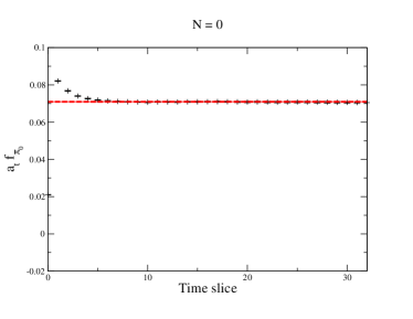
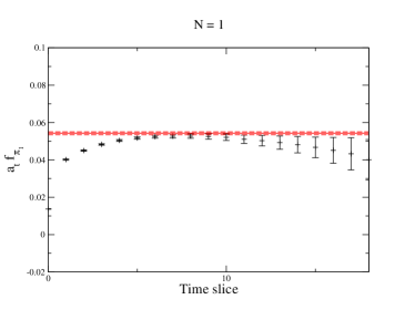
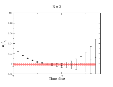
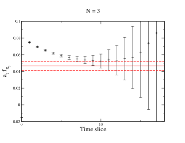
Figure 1: The data for $a_{t}f_{\pi_{N}}$ in units of the temporal lattice spacing from Eqn. (22), for the ensemble at $m_{\pi}=702~{}{\rm MeV}$; the line corresponds to the value of $a_{t}f_{\pi_{N}}$ obtained from a three-parameter fit to the data as discussed in the text. The optimal operators are obtained from the variational method with $t_{0}=7$ and the eigenvectors determined at $t_{\rm ref}=15$.

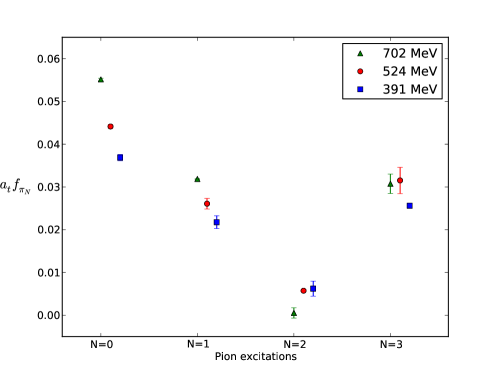
Figure 2: The unrenormalized pion decay constants $a_{t}f_{\pi_{N}}$ on each of our ensembles obtained using the unimproved axial-vector current.

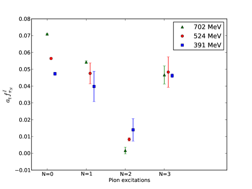
Figure 3: The unrenormalized pion decay constants $a_{t}f_{\pi_{N}}$ on each of our ensembles obtained using the improved axial-vector current.

The decay constants $a_{t}f_{\pi_{N}}$ for each of our ensembles computed using the unimproved and improved axial-vector currents is presented in Figures 2 and 3, respectively. We observe a decrease in the value of the decay constant up to and including that for the second excited state on all three ensembles, irrespective of the use of the unimproved or improved axial-vector current. In Figure 4, we show the ratio of the decay constant of the first excited state to that of the ground state, a combination in which the matching factor cancels, for both the unimproved (green) and improved (red) currents. Whilst we note that the improvement term represents a significant contribution at each quark mass, once again the behavior of the ratios remains the same for both currents.

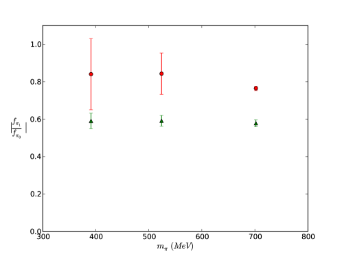
Figure 4: Lattice values for the ratio of the “improved” decay constants for the first excited $f_{\pi_{1}}$ and ground-state $f_{\pi_{0}}$ pion as a function of the pion mass. The green points represent unimproved values, while data in red color correspond to the ratios of improved decay constants.

So far, all lattice QCD predictions for the decay constant of the excitations of the pion have been made for the first excited state only. Here, we extend previous work through the calculation of the decay constant of higher excitations, up to that of the third excited state. The ratios $f_{\pi_{N}}/f_{\pi_{0}}$ of decay constants for the 1^st, 2^nd and 3^rd excited states to that of the ground state $f_{\pi_{0}}$ are shown using the unimproved and improved currents respectively in Figures 5 and 6, respectively.

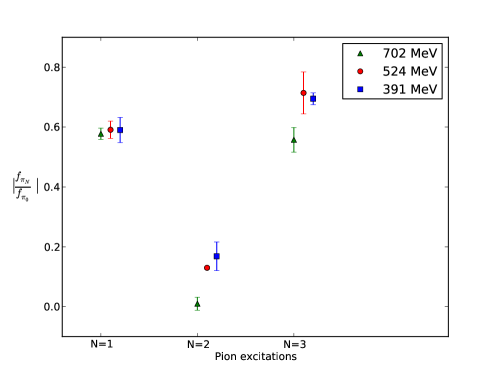
Figure 5: Ratios of the excited-state decay constants $f_{\pi_{N}}$ to the ground-state decay constant $f_{\pi_{0}}$ for the first three pion excitations ($N=1,\,2,\,3$), using the unimproved current.

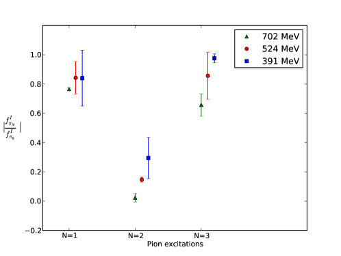
Figure 6: Ratios of the excited-state decay constants $f_{\pi_{N}}$ to the ground-state decay constant $f_{\pi_{0}}$ for the first 3 pion excitations ($N=1,\,2,\,3$), using the improved current.

Our results indicate the value of $\frac{f_{\pi 1}}{f_{\pi 0}}$ to be largely independent of the pion mass in the explored region of $400-700$ MeV. These conclusions differ from the previously mentioned lattice study performed by UKQCD Collaboration McNeile:2006qy . They find in particular that their results show a strong dependence on the current used. A simple linear fit to the ratio of the improved decay constants obtained through the implementation of the full ALPHA Collaboration method Jansen:1995ck gave $|f_{\pi_{1}}/f_{\pi_{0}}|=0.078(93)$ in the chiral limit, showing a significant suppression of the decay constant for the first pion excitation. Meanwhile, for the unimproved decay constants, they obtained $|f_{\pi_{1}}/f_{\pi_{0}}|=0.38(11)$ in the chiral limit. We have also employed an improved current, but the improvement term we include arises at tree level and is an artefact of the use of an anisotropic lattice.

A particularly striking observation is the strong suppression of the decay constant of the second excitation. The quark and gluon content of the excitations of the pion spectrum has been investigated earlier using the overlaps of the operators of the variational basis with the states in the spectrum as signatures for their partonic content Dudek:2010wm ; Dudek:2009qf , and a phenomenological interpretation provided in Ref. Dudek:2011pd . Of the lowest four states in the spectrum that we study here, each was identified as corresponding to a state of spin $0$ rather than of spin $4$, with the first excitation an $S$-wave radial excitation, but with the second excited state having a significant hybrid content represented by a strong overlap onto operators comprising a quark and antiquark coupled to a chromomagnetic field, as we illustrate for the lightest ensemble in Figure 7. Thus the strong suppression of the decay constant for the second-excited state, but the far more moderate suppression of the first excited state, is quite understandable within this phenomenology.

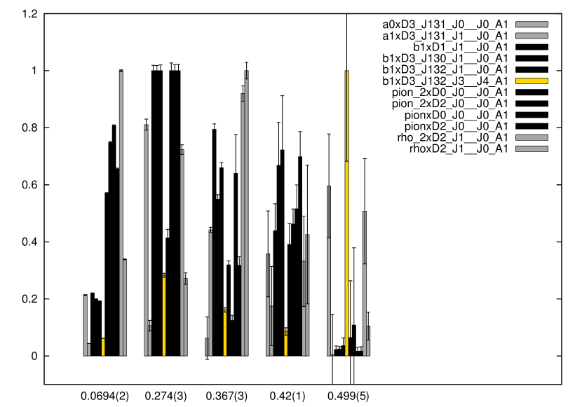
Figure 7: The histogram shows the overlap of the operators of the variational basis to the five lowest-lying states in the spectrum, for the data corresponding to a pion mass of $391~{}{\rm MeV}$, as described in Refs. Dudek:2010wm ; Dudek:2009qf . The yellow bar denotes the overlap onto an operator derived from a $J=4$ continuum construction; we associate the fourth excitation with a state of spin 4, and do not discuss further. Grey bars denote overlaps onto “hybrid” operators, as discussed in the text.

V Conclusions

In this work, we have undertaken the first steps in investigating the properties of the excited meson states in QCD by computing the decay constants both of the pion, and of its lowest three excitations. Our results show that the optimal operators obtained through the variational method are effective interpolating operators when calculating the hadron-to-vacuum matrix elements of local operators. The picture that emerges is that for the lowest two excitations, the decay constants are indeed suppressed, but largely independent of the quark mass, and that the strong suppression for the second excited state is indicative of the predominantly hybrid nature of the state.

The work presented here is highly encouraging, but there are certain caveats. Firstly, the basis of interpolating operators used here includes only “single-hadron” operators, whose coupling to multi-hadron decay states is expected to be suppressed by the volume, and thus our results effectively ignore that higher excitations become unstable under the strong interactions. Our previous work on the isovector spectrum suggested that the single-particle energy levels at these values of the quark mass are somewhat insensitive to the volume, but that has not been checked for the decay matrix elements. None-the-less, the fact that the decay constant ratios themselves show a limited quark-mass dependence, despite large differences in $m_{\pi}L$ ($L$ being the length of the lattice), leads credence to the results presented here. Secondly, the improvement term we include in the axial vector current is that arising at tree level through the use of an anisotropic action; mixings beyond tree level, and the matching coefficients, which cancel in the ratios of decays constants, have not been included. As well as addressing these issues, future work will extend the calculation to obtain the moments of the quark distribution amplitudes, and will investigate the decay constants and distribution amplitudes for both the $\rho$ and nucleon excitations.

VI Acknowledgements

We thank our colleagues within the Hadron Spectrum Collaboration, and in particular, Jo Dudek, Robert Edwards, Christian Shultz and Christopher Thomas. We are grateful for discussions with Zak Brown and Hannes L.L. Roberts, who was involved at an earlier stage of this work. Chroma Edwards:2004sx was used to perform this work on clusters at Jefferson Laboratory under the USQCD Initiative and the LQCD ARRA project. We acknowledge support from U.S. Department of Energy contract DE-AC05-06OR23177, under which Jefferson Science Associates, LLC, manages and operates Jefferson Laboratory.

Appendix A Axial-vector current improvement

Here we provide derivation of the formula for the improved axial-vector current that we use in our computations. Following closely the discussion on the classical improvement of the anisotropic action introduced in Ref. Chen:2001hq , we first start with the naive fermion action that has manifestly no $\mathcal{O}(a)$ discretization errors

$$\bar{\psi}_{c}(m_{c}+\not{\nabla})\psi_{c};$$

the bare quark mass $m_{c}$ here is the same as in the continuum. The $\mathcal{O}(a)$-improved anisotropic quark action can be derived by applying the field redefinition $\bar{\psi}_{c}=\bar{\psi}\,\bar{\Omega}$ ($\psi_{c}=\psi\,\Omega$), where

$$\Omega=1+\frac{\Omega_{m}}{2}a_{t}m_{c}+\frac{\Omega_{t}}{2}a_{t}\overrightarrow{\not{\nabla}}_{t}+\frac{\Omega_{s}}{2}a_{s}\overrightarrow{\bm{\not{\nabla}}},$$

$$\bar{\Omega}=1+\frac{\bar{\Omega}_{m}}{2}a_{t}m_{c}+\frac{\bar{\Omega}_{t}}{2}a_{t}\overleftarrow{\not{\nabla}}_{t}+\frac{\bar{\Omega}_{s}}{2}a_{s}\overleftarrow{\bm{\not{\nabla}}},$$ (23)

with $\Omega_{m,\,t,\,s}$ (and $\bar{\Omega}_{m,\,t,\,s}$) being mass-dependent pure numbers, and where the covariant lattice derivatives $\nabla_{\mu}$ are defined as

$$\nabla_{\mu}\psi(x)=\frac{1}{2a_{\mu}}\big{[}U_{\mu}(x)\psi(x+\mu)-U_{-\mu}(x)\psi(x-\mu)\big{]}.$$

The application of this field redefinition to the anisotropic action is discussed in detail in Ref. Chen:2001hq . Here we will focus on the improved quark-bilinear operators, given by

$$J^{I}=\bar{\psi}_{c}\Gamma\psi_{c}=\bar{\psi}\,\bar{\Omega}\,\Gamma\,\Omega\,\psi,$$ (24)

which, after substitution the formulae from Eqn. (23) and requiring $\Omega_{m}=\bar{\Omega}_{m}$, $\Omega_{t}=\bar{\Omega}_{t}$ and $\Omega_{s}=\bar{\Omega}_{s}$ (see Chen:2001hq ) turns into

$$J^{I} =(1+m_{c}a_{t}\Omega_{m})J^{U}+\frac{1}{2}\Omega_{t}a_{t}[\bar{\psi}\Gamma\overrightarrow{\not{\nabla}}_{t}\psi-\bar{\psi}\overleftarrow{\not{\nabla}}_{t}\Gamma\psi]+$$

$$+\frac{1}{2}\Omega_{s}a_{s}[\bar{\psi}\Gamma\overrightarrow{\bm{\not{\nabla}}}_{s}\psi-\bar{\psi}\overleftarrow{\bm{\not{\nabla}}}_{s}\Gamma\psi],$$ (25)

where $J^{U}\equiv\bar{\psi}\Gamma\psi$ is the unimproved operator.

For the case of the axial-vector current we have $\Gamma=\gamma_{\mu}\gamma_{5}$, and the improved axial-vector current current $A^{I}_{\mu}$ is given by

$$A_{\mu}^{I} =(1+\Omega_{m}a_{t}m_{c})A_{\mu}^{U}+\frac{\Omega_{t}a_{t}}{2}(\bar{\psi}\Gamma\overrightarrow{\not{\nabla}}_{t}\psi-\bar{\psi}\overleftarrow{\not{\nabla}}_{t}\Gamma\psi)+$$

$$+\frac{\Omega_{s}a_{s}}{2}(\bar{\psi}\Gamma\overrightarrow{\bm{\not{\nabla}}}_{s}\psi-\bar{\psi}\overleftarrow{\bm{\not{\nabla}}}_{s}\Gamma\psi)=$$

$$=(1+\Omega_{m}a_{t}m_{c})A_{\mu}^{U}+\frac{\Omega_{t}a_{t}}{2}(\bar{\psi}\gamma_{\mu}\gamma_{5}\gamma_{4}\overrightarrow{D}_{4}\psi-$$

$$-\bar{\psi}\gamma_{4}\gamma_{\mu}\gamma_{5}\overleftarrow{D}_{4}\psi)+\frac{\Omega_{s}a_{s}}{2}(\bar{\psi}\gamma_{\mu}\gamma_{5}\gamma_{j}\overrightarrow{D}_{j}\psi-$$

$$-\bar{\psi}\gamma_{j}\gamma_{\mu}\gamma_{5}\overleftarrow{D}_{j}\psi).$$ (26)

Using the relationship between the Euclidean gamma matrices and the Dirac matrices,

$$\gamma_{\mu}\gamma_{\nu}=\delta_{\mu\nu}+\sigma_{\mu\nu},$$ (27)

where

$$\sigma_{\mu\nu}=\frac{1}{2}[\gamma_{\mu},\ \gamma_{\nu}],$$ (28)

Eqn. (26) can be re-written as:

$$A_{\mu}^{I} =\big{(}1+\Omega_{m}a_{t}m_{c}\big{)}A_{\mu}^{U}-$$

$$-\frac{\Omega_{t}a_{t}}{2}\big{(}\bar{\psi}(\delta_{\mu 4}+\sigma_{\mu 4})\gamma_{5}\overrightarrow{D}_{4}\psi+\bar{\psi}(\delta_{4\mu}+\sigma_{4\mu})\gamma_{5}\overleftarrow{D}_{4}\psi\big{)}-$$

$$-\frac{\Omega_{s}a_{s}}{2}\big{(}\bar{\psi}(\delta_{\mu j}+\sigma_{\mu j})\gamma_{5}\overrightarrow{D}_{j}\psi+\bar{\psi}(\delta_{j\mu}+\sigma_{j\mu})\gamma_{5}\overleftarrow{D}_{j}\psi\big{)},$$ (29)

or

$$A_{\mu}^{I} =\big{(}1+\Omega_{m}a_{t}m_{c}\big{)}A_{\mu}^{U}+$$

$$+\frac{\Omega_{t}a_{t}}{2}\big{(}-\delta_{\mu 4}\partial_{4}\bar{\psi}\gamma_{5}\psi-\sigma_{\mu 4}\bar{\psi}\gamma_{5}\overrightarrow{D}_{4}\psi-\sigma_{4\mu}\bar{\psi}\gamma_{5}\overleftarrow{D}_{4}\psi\big{)}+$$

$$+\frac{\Omega_{s}a_{s}}{2}\big{(}-\delta_{\mu j}\partial_{j}\bar{\psi}\gamma_{5}\psi-\sigma_{\mu j}\bar{\psi}\gamma_{5}\overrightarrow{D}_{j}\psi-\sigma_{j\mu}\bar{\psi}\gamma_{5}\overleftarrow{D}_{j}\psi\big{)}$$ (30)

To simplify this expression, we make use of the equations of motion which (to the lowest order) are written as:

$$(m_{0}+\nu_{t}\overrightarrow{\not{D}}_{t}+\nu_{s}\overrightarrow{\not{D}}_{s})\psi=0,$$ (31)

$$\bar{\psi}(m_{0}-\nu_{t}\overleftarrow{\not{D}}_{t}-\nu_{s}\overleftarrow{\not{D}}_{s})=0.$$ (32)

From the first equation:

$$m_{0}\gamma_{\rho}\psi+\nu_{t}\gamma_{\rho}\gamma_{4}\overrightarrow{D}_{4}\psi+\nu_{s}\gamma_{\rho}\gamma_{j}\overrightarrow{D}_{j}\psi=0,$$ (33)

and therefore

$$\nu_{s}\sigma_{\rho j}\overrightarrow{D}_{j}\psi+\nu_{t}\sigma_{\rho 4}\overrightarrow{D}_{4}\psi=-m_{0}\gamma_{\rho}\psi-\nu_{t}\delta_{\rho 4}\overrightarrow{D}_{4}\psi-\nu_{s}\delta_{\rho j}\overrightarrow{D}_{j}\psi.$$ (34)

Similarly, from Eqn. (32) we get:

$$m_{0}\bar{\psi}\gamma_{\rho}-\nu_{t}\bar{\psi}\gamma_{4}\gamma_{\rho}\overleftarrow{D}_{4}-\nu_{s}\bar{\psi}\gamma_{j}\gamma_{\rho}\overleftarrow{D}_{j}=0,$$ (35)

and

$$\nu_{t}\bar{\psi}\sigma_{4\rho}\overleftarrow{D}_{4}+\nu_{s}\bar{\psi}\sigma_{j\rho}\overleftarrow{D}_{j}=m_{0}\bar{\psi}\gamma_{\rho}-\nu_{t}\bar{\psi}\delta_{4\rho}\overleftarrow{D}_{4}-\nu_{s}\bar{\psi}\delta_{j\rho}\overleftarrow{D}_{j}.$$ (36)

Here we consider the temporal component of the axial-vector current ($\mu=4$), so Eqn. (30) becomes

$$A_{4}^{I} =\big{(}1+\Omega_{m}a_{t}m_{c}\big{)}A_{4}^{U}-\frac{\Omega_{t}a_{t}}{2}\delta_{\rho 4}\partial_{4}\bar{\psi}\gamma_{5}\psi-$$

$$-\frac{\Omega_{s}a_{s}}{2}\big{(}\sigma_{4j}\bar{\psi}\gamma_{5}\overrightarrow{D}_{j}\psi+\sigma_{j4}\bar{\psi}\gamma_{5}\overleftarrow{D}_{j}\psi\big{)}$$ (37)

and, after applying Eqns. (34) and (36), we obtain:

$$A_{4}^{I}=(1+\Omega_{m}a_{t}m_{c})A_{4}^{U}+\frac{a_{t}}{2}\big{(}\Omega_{s}\frac{a_{s}}{a_{t}}\frac{\nu_{t}}{\nu_{s}}-\Omega_{t}\big{)}\partial_{4}\bar{\psi}\gamma_{5}\psi.$$ (38)

We choose the case with $\nu_{t}=1$ (so-called “$\nu_{s}$-tuning”), where $\nu_{s}$ is tuned via the dispersion relation between meson energy and momentum, yielding

$$\nu_{s}=\frac{1+\frac{1}{2}a_{t}m_{c}}{1+\frac{1}{2}a_{s}m_{c}}.$$ (39)

The parameters $\Omega_{t}$ and $\Omega_{s}$ are set as in Ref. Chen:2001hq :

$$\Omega_{s}=-\frac{1}{2}\left(\frac{1+\frac{1}{2}a_{t}m_{c}}{1+\frac{1}{2}a_{s}m_{c}}\right),\,\,\,\Omega_{t}=-\frac{1}{2}.$$ (40)

The value for the anisotropy parameter in our calculations is $\xi=\frac{a_{s}}{a_{t}}\approx 3.5$, so the final expression for the time component of the improved axial-vector current takes the form:

$$A_{4}^{I}=(1+\Omega_{m}a_{t}m_{c})A_{4}^{U}-0.625\,a_{t}\partial_{4}\bar{\psi}\gamma_{5}\psi,$$ (41)

or, up to leading order in $a$,

$$A_{4}^{I}=(1+\Omega_{m}a_{t}m_{c})\left[A_{4}^{U}-\frac{1}{4}(\xi-1)a_{t}\partial_{4}P\right].$$ (42)

References

- (1) J. Dudek, R. Ent, R. Essig, K. Kumar, C. Meyer, et al., Eur.Phys.J. A48, 187 (2012), arXiv:1208.1244 [hep-ex]
- (2) J. J. Dudek, R. G. Edwards, M. J. Peardon, D. G. Richards, and C. E. Thomas, Phys.Rev.Lett. 103, 262001 (2009), arXiv:0909.0200 [hep-ph]
- (3) J. J. Dudek, R. G. Edwards, M. J. Peardon, D. G. Richards, and C. E. Thomas, Phys.Rev. D82, 034508 (2010), arXiv:1004.4930 [hep-ph]
- (4) J. J. Dudek, Phys. Rev. D 84, 074023 (Oct 2011), http://link.aps.org/doi/10.1103/PhysRevD.84.074023
- (5) J. J. Dudek, R. G. Edwards, B. Joo, M. J. Peardon, D. G. Richards, et al., Phys.Rev. D83, 111502 (2011), arXiv:1102.4299 [hep-lat]
- (6) J. J. Dudek and R. G. Edwards, Phys. Rev. D 85, 054016 (Mar 2012), http://link.aps.org/doi/10.1103/PhysRevD.85.054016
- (7) S. Weinberg, Physica A: Statistical Mechanics and its Applications 96A, 327 (1979), ISSN 0378-4371, http://www.sciencedirect.com/science/article/pii/0378437179902231
- (8) J. Gasser and H. Leutwyler, Annals of Physics 158, 142 (1984), ISSN 0003-4916, http://www.sciencedirect.com/science/article/pii/0003491684902422
- (9) J. Beringer et al. (Particle Data Group), Phys.Rev. D86, 010001 (2012)
- (10) E. Follana, C. T. H. Davies, G. P. Lepage, and J. Shigemitsu (HPQCD and UKQCD Collaborations), Phys. Rev. Lett. 100, 062002 (Feb 2008), http://link.aps.org/doi/10.1103/PhysRevLett.100.062002
- (11) S. Durr, Z. Fodor, C. Hoelbling, S. Katz, S. Krieg, et al., Phys.Rev. D81, 054507 (2010), arXiv:1001.4692 [hep-lat]
- (12) A. Bazavov et al. (MILC Collaboration), PoS LATTICE2010, 074 (2010), arXiv:1012.0868 [hep-lat]
- (13) R. Dowdall, C. Davies, G. Lepage, and C. McNeile, Phys.Rev. D88, 074504 (2013), arXiv:1303.1670 [hep-lat]
- (14) A. Holl, A. Krassnigg, and C. Roberts, Phys.Rev. C70, 042203 (2004), arXiv:nucl-th/0406030 [nucl-th]
- (15) M. Volkov and C. Weiss, Phys.Rev. D56, 221 (1997), arXiv:hep-ph/9608347 [hep-ph]
- (16) L. Chang, C. D. Roberts, and P. C. Tandy, Chin.J.Phys. 49, 955 (2011), arXiv:1107.4003 [nucl-th]
- (17) C. McNeile and C. Michael (UKQCD Collaboration), Phys.Lett. B642, 244 (2006), arXiv:hep-lat/0607032 [hep-lat]
- (18) C. Michael, Nuclear Physics B 259, 58 (1985), ISSN 0550-3213, http://www.sciencedirect.com/science/article/pii/0550321385902974
- (19) M. Luscher and U. Wolff, Nucl.Phys. B339, 222 (1990)
- (20) B. Blossier, M. Della Morte, G. von Hippel, T. Mendes, and R. Sommer, JHEP 0904, 094 (2009), arXiv:0902.1265 [hep-lat]
- (21) M. Peardon et al. (Hadron Spectrum Collaboration), Phys.Rev. D80, 054506 (2009), arXiv:0905.2160 [hep-lat]
- (22) R. G. Edwards, B. Joo, and H.-W. Lin, Phys.Rev. D78, 054501 (2008), arXiv:0803.3960 [hep-lat]
- (23) H.-W. Lin, S. D. Cohen, J. Dudek, R. G. Edwards, B. Joó, D. G. Richards, J. Bulava, J. Foley, C. Morningstar, E. Engelson, S. Wallace, K. J. Juge, N. Mathur, M. J. Peardon, and S. M. Ryan (Hadron Spectrum Collaboration), Phys. Rev. D 79, 034502 (Feb 2009), http://link.aps.org/doi/10.1103/PhysRevD.79.034502
- (24) J. Bulava, R. Edwards, E. Engelson, B. Joo, H.-W. Lin, et al., Phys.Rev. D82, 014507 (2010), arXiv:1004.5072 [hep-lat]
- (25) J. J. Dudek, R. Edwards, and C. E. Thomas, Phys.Rev. D79, 094504 (2009), arXiv:0902.2241 [hep-ph]
- (26) J. J. Dudek, R. G. Edwards, P. Guo, and C. E. Thomas, Phys. Rev. D 88, 094505, 094505 (2013), arXiv:1309.2608 [hep-lat]
- (27) G. Moir, M. Peardon, S. M. Ryan, C. E. Thomas, and L. Liu, JHEP 1305, 021 (2013), arXiv:1301.7670 [hep-ph]
- (28) L. Liu et al. (Hadron Spectrum Collaboration), JHEP 1207, 126 (2012), arXiv:1204.5425 [hep-ph]
- (29) R. G. Edwards, J. J. Dudek, D. G. Richards, and S. J. Wallace, Phys.Rev. D84, 074508 (2011), arXiv:1104.5152 [hep-ph]
- (30) J. J. Dudek and R. G. Edwards, Phys.Rev. D85, 054016 (2012), arXiv:1201.2349 [hep-ph]
- (31) R. G. Edwards, N. Mathur, D. G. Richards, and S. J. Wallace, Phys.Rev. D87, 054506 (2013), arXiv:1212.5236 [hep-ph]
- (32) M. Padmanath, R. G. Edwards, N. Mathur, and M. Peardon(2013), arXiv:1307.7022 [hep-lat]
- (33) P. Chen, Phys. Rev. D 64, 034509 (Jul 2001), http://link.aps.org/doi/10.1103/PhysRevD.64.034509
- (34) J. J. Dudek, R. G. Edwards, and D. G. Richards, Phys.Rev. D73, 074507 (2006), arXiv:hep-ph/0601137 [hep-ph]
- (35) S.-x. Qin, L. Chang, Y.-x. Liu, C. D. Roberts, and D. J. Wilson, Phys.Rev. C85, 035202 (2012), arXiv:1109.3459 [nucl-th]
- (36) A. Holl, A. Krassnigg, P. Maris, C. Roberts, and S. Wright, Phys.Rev. C71, 065204 (2005), arXiv:nucl-th/0503043 [nucl-th]
- (37) K. Jansen, C. Liu, M. Luscher, H. Simma, S. Sint, et al., Phys.Lett. B372, 275 (1996), arXiv:hep-lat/9512009 [hep-lat]
- (38) R. G. Edwards and B. Joo (SciDAC Collaboration, LHPC Collaboration, UKQCD Collaboration), Nucl.Phys.Proc.Suppl. 140, 832 (2005), arXiv:hep-lat/0409003 [hep-lat]