Pick and freeze estimation of sensitivity indices for models with dependent and dynamic input processes

Abstract

This paper addresses sensitivity analysis for dynamic models, linking dependent inputs to observed outputs. The usual method to estimate Sobol indices are based on the independence of input variables. We present a method to overpass this constraint when inputs are Gaussian processes of high dimension in a time related framework. Our proposition leads to a generalization of Sobol indices when inputs are both dependant and dynamic. The method of estimation is a modification of the Pick and Freeze simulation scheme. First we study the general Gaussian cases and secondly we detail the case of stationary models. We then apply the results to an example of heat exchanges inside a building.

1 Introduction

To study physical phenomena, it is useful to build mathematic models which translate them. These models can be used for purposes such as managements or forecasts for example. So it is important for the practitioner to assess the fiability of the models used. The sources of uncertainties in a model may be located at two levels :

• on the parameters when they are estimated them for example

• on the inputs of the model (error of measures, variability of the inputs,$\displaystyle\dots$)

Sensitivity analysis can help to do this work. It aims to quantify uncertainties of each factor on the output of the model. The interest can notably be to :

• reduce variability of the output

• prioritize factors : see which factor is the most influent on the output and need more precision on its estimation or its measure

• calibrate the least influent factors.

Among the tools available in global stochastic sensitivity analysis (see for example [1] and references therein), the most used one is Sobol index defined if the variables are assumed to be independent random variables. Their probability distributions account for the practitioner’s belief in the input uncertainty. This turns the model output into a random variable, whose total variance can be split down into different partial variances (this is the so-called Hoeffding decomposition, also known as functional ANOVA, see [2]). Each partial variance is defined as the variance of the conditional expectation of the output with respect to each input variable. By considering the ratio of each partial variance to the total variance, we obtain the Sobol sensitivity index of the variable [3, 4]. This index quantifies the impact of the variability of the factor on the output. Its value is between 0 and 1 allowing to prioritize the variables according to their influence.

Even when the inputs are not independent, it seems reasonable to consider the same Sobol index but with a quite different interpretation. Several approaches have been proposed in the literature about dependent inputs. In their introduction, Mara et al. [5] cite some of them, which are claimed to be relevant only in the case of a linear model. In that paper, the authors introduce an estimation method for the Sobol index but this method seems computationally intricate. On the other hand, Kucherenko et al. [6] rewrite, as we will do, the Sobol index as a covariance between the output and a copy of the output. Another method ([7]) modifies the Sobol index definition, which leads to indices that are hard to estimate, as well as results that may seem counter-intuitive (for instance, the indices may not be between 0 and 1).

Few works propose to study the sensitivity to dynamic inputs. The sensitivity is calculated at each time step $\displaystyle t$ without taking into account the dynamic behaviour of the input. Indeed, the impact of the variability is not always instantaneous. It seems necessary to develop a new method to dynamic dependent inputs. In this way, the Sobol index definition is modified.

We set ourselves in a time related framework and we study the following scalar output $\displaystyle Y$ :

$$Y_{t}=f_{t}\left((\mbox{\boldmath{$\displaystyle U$}}_{s})_{0\leq s\leq t}\right),\;\;\;t\in\mathbb{N}$$ (1)

The input is a vectorial Gaussian process $\displaystyle(\mbox{\boldmath{$U$}}_{s})_{s\in\mathbb{N}}\subset\mathbb{R}^{p}$. In this context, the sensitivity is defined for $\displaystyle Y_{t}$ with respect to the input process $\displaystyle(U^{1}_{s})_{0\leq s\leq t}$ (for example). Thus the sensitivity changes with time $\displaystyle t$. The dynamic framework is the most useful in stationary or almost stationary cases. In non stationary cases the problem is no more that a sequence of finite dimensional situations. We focus on two cases with $\displaystyle\mbox{\boldmath{$U$}}_{t}$ a stationary process :

• $\displaystyle Y_{t}=f(\mbox{\boldmath{$U$}}_{t},\mbox{\boldmath{$U$}}_{t-1},\dots,\mbox{\boldmath{$U$}}_{t-M})$ for some $\displaystyle M$

• $\displaystyle Y_{t}=f(\mbox{\boldmath{$U$}}_{t},\mbox{\boldmath{$U$}}_{t-1},\dots,\mbox{\boldmath{$U$}}_{0},0,\dots,0)$ deduced from a stationary process given by
  $\displaystyle Y^{\star}_{t}=f(\mbox{\boldmath{$U$}}_{t},\mbox{\boldmath{$U$}}_{t-1},\dots,\mbox{\boldmath{$U$}}_{0},\mbox{\boldmath{$U$}}_{-1},\dots)$.
  This case includes models associated to recurrence equations as Euler schemes of stochastic differential equations.

The method of estimation that seems best suited for functional multidimensional models is the Pick and Freeze scheme (see [4, 8]). It allows flexibility in the form of the inputs and doesn’t care of the number of variables by which it is desired to condition the variance, the only constraint being the assumption of independent inputs. In SPF (Scheme Pick and Freeze), a Sobol index is viewed as the correlation coefficient between the output of the model and its pick-freezed replication. This replication is obtained by holding the value of the variable of interest (frozen variable) and by sampling the other variables (picked variables). The sampled replications are then combined to produce an estimator of the Sobol index.

In a first part, after reminding the definition of Sobol index and the Pick and Freeze scheme, we introduce the definition of the index in a dynamic case. We show that under the hypothesis of Gaussian inputs, it is possible to reduce this problem to the case of independent variables and apply the method Pick and Freeze. In the second part we present the properties of our index when inputs are stationary. Finally an application to a physical problem is presented in the last section.

Notations

Let us give some notations :

• $\displaystyle X,Z$ random variables

• $\displaystyle\mbox{\boldmath{$U$}},\mbox{\boldmath{$Z$}}$ random vectors

• $\displaystyle\left(\mbox{\boldmath{$U$}}_{t}\right)_{t\in\mathbb{N}}$ a vectorial process, $\displaystyle dim(\mbox{\boldmath{$U$}}_{t})=p$

• $\displaystyle\mbox{\boldmath{$U$}}_{\lfloor a,b\rfloor}=\left\{\mbox{\boldmath{$U$}}_{s},a\leq s\leq b\right\}$, $\displaystyle p\times(b-a+1)$ matrix, with $\displaystyle-\infty\leq a\leq b\leq+\infty$

• $\displaystyle\mbox{\boldmath{$U$}}^{*}$ or $\displaystyle\mbox{\boldmath{$U$}}_{t}^{*}$ is the transposed vector of $U$ or the vectorial process $\displaystyle\mbox{\boldmath{$U$}}_{t}$

If $\displaystyle X_{t}$ and $\displaystyle\mbox{\boldmath{$Z$}}_{t}$ are two stochastic vectorial centered processes with $\displaystyle dim(X_{t})=1,\;dim(\mbox{\boldmath{$Z$}}_{t})=p-1$, we define different covariance matrices as following :

Definition 1.

$\displaystyle\gamma_{s,v}^{XZ^{j}}=\mathbf{E}(X_{s}Z^{j}_{v})$ the covariance between $\displaystyle X_{s}$ and $\displaystyle Z^{j}_{v}$ where $\displaystyle j$ denotes the jth component of the vector $\displaystyle\mbox{\boldmath{$Z$}}_{v}$

Definition 2.

$\displaystyle\mbox{\boldmath{$\gamma$}}_{\lfloor 0,t\rfloor,v}^{XZ^{j}}=\mathbf{E}(X_{\lfloor 0,t\rfloor}Z^{j}_{v})$ a $\displaystyle(t+1)$ vector process of generic term $\displaystyle\gamma_{s,v}^{XZ^{j}},\;\;0\leq s\leq t$

Definition 3.

$\displaystyle\Gamma_{\lfloor 0,t\rfloor,v}^{XZ}$ the $\displaystyle(t+1)\times(p-1)$ covariance matrix of generic term $\displaystyle\mbox{\boldmath{$\gamma$}}_{\lfloor 0,t\rfloor,v}^{XZ^{j}}$ for $\displaystyle 1\leq j\leq p-1,\;0\leq s\leq t$

Definition 4.

$\displaystyle\Gamma_{\lfloor 0,t\rfloor,\lfloor 0,u\rfloor}^{XZ}$ the $\displaystyle(t+1)\times(p-1)(u+1)$ matrix using matrix blocks $\displaystyle\Gamma^{XZ}_{\lfloor 0,t\rfloor,v}$ with $\displaystyle 0\leq v\leq u$

To simplify the exposition we consider an input vector $\displaystyle\mbox{\boldmath{$U$}}=(U^{1},\dots,U^{2})$. We denote by $\displaystyle X=U^{1}$ and $\displaystyle\mbox{\boldmath{$Z$}}=\left(U^{2},\dots,U^{p}\right)$ when we are in static context and $\displaystyle X_{t}=U_{t}^{1}$ and $\displaystyle\mbox{\boldmath{$Z$}}_{t}=\left(U_{t}^{2},\dots,U_{t}^{p}\right)$ in the dynamic case.

2 Sobol indices : extended definition and estimation

2.1 Definition in a dynamic context

We consider the model given by : $\displaystyle Y=f(\mbox{\boldmath{$U$}})$, $\displaystyle\mbox{\boldmath{$U$}}\in\mathbb{R}^{p}$ is a random vector with known distributions. We assume that all coordinates of $U$ and $\displaystyle Y$ have a finite non zero variance.

The Sobol index with respect to $\displaystyle X$ is defined by [3] :

$$S^{X}=\frac{\mathbf{Var}\left(\mathbf{E}(Y|X)\right)}{\mathbf{Var}(Y)}.$$ (2)

$\displaystyle S^{X}$ is the Sobol index with respect to $\displaystyle X$. More generally, $\displaystyle S^{J}$ is the closed Sobol index with respect to the group $\displaystyle J$ of variables $\displaystyle\mbox{\boldmath{$U$}}^{J}=\left(U^{j},j\in J\right)$ :

$$S^{U^{J}}=\frac{\mathbf{Var}\left(\mathbf{E}(Y|\mbox{\boldmath{$\displaystyle U$}}^{J})\right)}{\mathbf{Var}(Y)}.$$ (3)

Total indices and higher-order Sobol indices can also be written by taking the sum or the difference of closed indices. Hence, we can restrict ourselves to the case of two (possibly vector) inputs in the model.

We now introduce the time dimension and we define the input-output relation :

$$Y_{t}=f_{t}((\mbox{\boldmath{$\displaystyle U$}}_{s})_{0\leq s\leq t})$$ (4)

$\displaystyle(\mbox{\boldmath{$U$}}_{s})_{s\in\mathbb{N}}\subset\mathbb{R}^{p}$ is a vector-valued stochastic process, $\displaystyle f_{t}$ being a sequence of functions which will be detailed later. Let $\displaystyle\mbox{\boldmath{$U$}}_{t}=(X_{t},\mbox{\boldmath{$Z$}}_{t})$ with $\displaystyle X_{t}=U^{1}_{t}$ and $\displaystyle\mbox{\boldmath{$Z$}}_{t}=(U^{2}_{t},\dots,U^{p}_{t})$.

For each $\displaystyle t\in\mathbb{N}$, we define a measure of the sensitivity of $\displaystyle Y_{t}$ with respect to $\displaystyle X_{\lfloor 0,t\rfloor}=(X_{0},\dots,X_{t-1},X_{t})$ by :

$$S^{X}_{t}=\frac{\mathbf{Var}\left(\mathbf{E}\left(Y_{t}|X_{\lfloor 0,t\rfloor}\right)\right)}{\mathbf{Var}(Y_{t})}$$ (5)

The index $\displaystyle t\mapsto S^{X}_{t}$ is called the projection on the past sensitivity index with respect to $\displaystyle X$. We notice that, at any given time $\displaystyle t$, we consider the sensitivity of $\displaystyle Y_{t}$ with respect to all the past $\displaystyle X_{\lfloor 0,t\rfloor}$ values of the $\displaystyle X$ process, not just its value $\displaystyle X_{t}$.

Of course, the conditional expectation with respect to $\displaystyle X_{\lfloor 0,t\rfloor}$ takes into account the dependence of $\displaystyle\mbox{\boldmath{$Z$}}_{\lfloor 0,t\rfloor}$ with respect to $\displaystyle X_{\lfloor 0,t\rfloor}$.

Remark 1.

When the inputs are dependent we keep the property that $\displaystyle S^{X}_{t}\leq 1$ for any $\displaystyle t$. The classical term of interaction $\displaystyle S^{XZ}$ is not defined [9].

2.2 Estimation of $\displaystyle S^{X}$, the Pick and Freeze method in the independent case

There exists many methods for estimating $\displaystyle S^{X}$. One of them is the so-called Pick and Freeze scheme [4, 3]. In this case $\displaystyle f$ plays the role of a black box allowing to simulate the input-output relationship without any mathematical description. This method is based on the following lemma [4] :

Lemma 1.

Sobol : Let $\displaystyle\mbox{\boldmath{$U$}}=(X,\mbox{\boldmath{$Z$}})$. If $\displaystyle X$ and $Z$ are independent :

$$\mathbf{Var}(\mathbf{E}(Y|X))=\mathbf{Cov}(Y,Y^{X})$$

with $\displaystyle Y^{X}=f(X,\mbox{\boldmath{$Z$}}^{\prime}),Y=f(X,\mbox{\boldmath{$Z$}})$ where $\displaystyle\mbox{\boldmath{$Z$}}^{\prime}$ is an independent copy of $Z$.

We can deduce the expression of $\displaystyle S^{X}$ when $\displaystyle X$ and $Z$ are independent :

$$S^{X}=\frac{\mathbf{Cov}(Y,Y^{X})}{\mathbf{Var}(Y)},$$ (6)

A natural estimator consists in taking the empirical estimators of the covariance and of the variance. Let a $\displaystyle N-$sample $\displaystyle\{(Y^{(1)},Y^{X,(1)}),\dots,(Y^{(N)},Y^{X,(N)})\}$ a natural estimator of $\displaystyle S^{X}$ is :

$$\widehat{S}^{X}=\frac{\frac{1}{N}\sum_{i=1}^{N}Y^{(i)}Y^{X,(i)}-(\frac{1}{N}\sum_{i=1}^{N}Y^{(i)})(\frac{1}{N}\sum_{i=1}^{N}Y^{X,(i)})}{\frac{1}{N}\sum_{i=1}^{N}(Y^{(i)})^{2}-(\frac{1}{N}\sum_{i=1}^{N}Y^{(i)})^{2}}$$ (7)

If $\displaystyle X$ and $Z$ are finite dimensional random vectors this formula can be justified by asymptotic properties when $\displaystyle N\rightarrow\infty$. The speed of convergence of this estimator is in $\displaystyle O(1/\sqrt{N})$, see Janon et al. [10]. In practice it can be approximated by $\displaystyle\frac{C}{\sqrt{N}}$ where $\displaystyle C$ can be large as we will see later.

In the dependent case the estimation of $\displaystyle S^{X}_{t}$ by a Monte-Carlo method is a challenging task, as one cannot be chosen $\displaystyle X=(X_{\lfloor 0,t\rfloor})$ and $\displaystyle\mbox{\boldmath{$Z$}}=(\mbox{\boldmath{$Z$}}_{\lfloor 0,t\rfloor})$ in (6) since $\displaystyle X$ and $Z$ are not independent. However, we will see, in the following Section, that, in a particular Gaussian case, whatever the covariance structure is, an efficient Pick and Freeze scheme may be built.

2.3 Reduction to independent inputs for Gaussian processes

Suppose that we are able to get another expression of the $\displaystyle Y_{t}$ output of the type :

$$Y_{t}=g_{t}(X_{\lfloor 0,t\rfloor},\mbox{\boldmath{$\displaystyle W$}}_{\lfloor 0,t\rfloor})$$ (8)

where $\displaystyle\mbox{\boldmath{$W$}}_{\lfloor 0,t\rfloor}$ is a stochastic process independent of $\displaystyle X_{\lfloor 0,t\rfloor}$, $\displaystyle\mbox{\boldmath{$W$}}_{\lfloor 0,t\rfloor}$ being $\displaystyle(X_{s},\mbox{\boldmath{$Z$}}_{s})_{s\leq t}$ measurable.

Then :

$$S^{X}_{t}=\frac{\mathbf{Var}\left(\mathbf{E}\left(Y_{t}=g_{t}(X_{\lfloor 0,t\rfloor},\mbox{\boldmath{$\displaystyle W$}}_{\lfloor 0,t\rfloor})|X_{\lfloor 0,t\rfloor}\right)\right)}{\mathbf{Var}(Y_{t})}$$ (9)

is defined as in the classical case of independence.

We now prove that if $\displaystyle Y_{t}=f_{t}(\mbox{\boldmath{$U$}}_{t},\mbox{\boldmath{$U$}}_{t-1},\dots,\mbox{\boldmath{$U$}}_{0})$ there exists $\displaystyle g_{t}$ satisfying (8).

Let :

$$\displaystyle\tilde{\mbox{\boldmath{$X$}}}_{t}=\mathbf{E}\left(\mbox{\boldmath{$Z$}}_{t}|X_{\lfloor 0,t\rfloor}\right)=\Lambda X_{\lfloor 0,t\rfloor}\mbox{ for a matrix }\Lambda\mbox{ with }dim(\Lambda)=(p-1)\times(t+1),$$

$$\displaystyle\text{and }\mbox{\boldmath{$W$}}_{t}=\mbox{\boldmath{$Z$}}_{t}-\mathbf{E}\left(\mbox{\boldmath{$Z$}}_{t}|X_{\lfloor 0,t\rfloor}\right)$$

Independence of $\displaystyle X_{\lfloor 0,t\rfloor}$ and $\displaystyle\mbox{\boldmath{$W$}}_{\lfloor 0,t\rfloor}$ holds thanks to the Gaussian assumption.

Let :

$$\displaystyle f_{t}(X_{\lfloor 0,t\rfloor},\mbox{\boldmath{$Z$}}_{\lfloor 0,t\rfloor}) \displaystyle=f_{t}(X_{\lfloor 0,t\rfloor},\tilde{\mbox{\boldmath{$X$}}}_{\lfloor 0,t\rfloor}+\mbox{\boldmath{$W$}}_{\lfloor 0,t\rfloor})$$ (10)

$$\displaystyle=f_{t}(X_{\lfloor 0,t\rfloor},\Lambda X_{\lfloor 0,t\rfloor}+\mbox{\boldmath{$W$}}_{\lfloor 0,t\rfloor})$$ (11)

$$\displaystyle=g_{t}(X_{\lfloor 0,t\rfloor},\mbox{\boldmath{$W$}}_{\lfloor 0,t\rfloor})$$ (12)

Let us now compute $\displaystyle\tilde{\mbox{\boldmath{$X$}}}_{\lfloor 0,t\rfloor}$ defined as :

$$\mathbf{E}(\mbox{\boldmath{$Z$}}_{\lfloor 0,t\rfloor}|X_{\lfloor 0,t\rfloor})=\left\{\mathbf{E}(\mbox{\boldmath{$Z$}}_{u}|X_{\lfloor 0,t\rfloor}),\;0\leq u\leq t\right\}=\tilde{\mbox{\boldmath{$X$}}}_{\lfloor 0,t\rfloor}$$

$\displaystyle(X_{t},\mbox{\boldmath{$Z$}}_{t})$ being a Gaussian vector, conditional expectations with respect to $\displaystyle X_{\lfloor 0,t\rfloor}$ are the projections on the linear space generated by $\displaystyle X_{\lfloor 0,t\rfloor}$.

Assumption 1.

For every $\displaystyle t$ we suppose that $\displaystyle\mbox{\boldmath{$U$}}_{\lfloor 0,t\rfloor}$ is of full rank.

Thus :

$$\mathbf{E}(Z_{u}^{j}|X_{\lfloor 0,t\rfloor})=\mbox{\boldmath{$\displaystyle\lambda$}}^{j}_{\lfloor 0,t\rfloor,u}X^{*}_{\lfloor 0,t\rfloor}$$ (13)

where $\displaystyle\mbox{\boldmath{$\lambda$}}^{j}_{\lfloor 0,t\rfloor,u}$ is a vector of size $\displaystyle(t+1)$ given by classical linear regression results :

$$\mbox{\boldmath{$\displaystyle\lambda$}}^{j}_{\lfloor 0,t\rfloor,u}=\left(\Gamma^{XX}_{\lfloor 0,t\rfloor,\lfloor 0,t\rfloor}\right)^{-1}\gamma^{XZ^{j}}_{\lfloor 0,t\rfloor,u}$$ (14)

$\displaystyle\Gamma^{XX}_{\lfloor 0,t\rfloor,\lfloor 0,t\rfloor}$ is invertible as consequence of assumption 1.

Let $\displaystyle\Gamma_{\lfloor 0,t\rfloor,\lfloor 0,t\rfloor}^{X,Z}$ defined as previously in (3) and

$$\Lambda^{XZ}_{\lfloor 0,t\rfloor,\lfloor 0,t\rfloor}=\left(\Gamma^{XX}_{\lfloor 0,t\rfloor,\lfloor 0,t\rfloor}\right)^{-1}\Gamma^{XZ}_{\lfloor 0,t\rfloor,\lfloor 0,t\rfloor}$$ (15)

then :

$$\tilde{\mbox{\boldmath{$\displaystyle X$}}}_{\lfloor 0,t\rfloor}=\Lambda^{XZ}_{\lfloor 0,t\rfloor,\lfloor 0,t\rfloor}X_{\lfloor 0,t\rfloor}$$ (16)

$\displaystyle\tilde{\mbox{\boldmath{$X$}}}_{\lfloor 0,t\rfloor}$ is a $\displaystyle(p-1)\times(t+1)$ matrix as is $\displaystyle\mbox{\boldmath{$W$}}_{\lfloor 0,t\rfloor}=\mbox{\boldmath{$Z$}}_{\lfloor 0,t\rfloor}-\tilde{\mbox{\boldmath{$X$}}}_{\lfloor 0,t\rfloor}$.

Thanks to (10) we have :

$$S^{X}_{t}=\frac{\mathbf{Var}\left(\mathbf{E}\left(g_{t}(X_{\lfloor 0,t\rfloor},\mbox{\boldmath{$W$}}_{\lfloor 0,t\rfloor})|X_{\lfloor 0,t\rfloor}\right)\right)}{\mathbf{Var}(Y_{t})}.$$

Note that the space of all the square integrable functions of the form $\displaystyle\phi(X_{\lfloor 0,t\rfloor})$ is the same as the space of all the square integrable function of the form $\displaystyle\psi(X_{\lfloor 0,t\rfloor},\tilde{\mbox{\boldmath{$X$}}}_{\lfloor 0,t\rfloor})$.
Thus $\displaystyle\mathbf{E}(Y_{t}|(X_{\lfloor 0,t\rfloor},\tilde{\mbox{\boldmath{$X$}}}_{\lfloor 0,t\rfloor}))=\mathbf{E}(Y_{t}|X_{\lfloor 0,t\rfloor})$. For $\displaystyle t$ fixed, we are now exactly in the previous case of two groups of independent inputs $\displaystyle X_{\lfloor 0,t\rfloor}$ and $\displaystyle\mbox{\boldmath{$W$}}_{\lfloor 0,t\rfloor}$ and thus we can apply the Pick and Freeze method (10) and (6) with $\displaystyle\mbox{\boldmath{$X$}}=\left(X_{\lfloor 0,t\rfloor},\tilde{\mbox{\boldmath{$X$}}}_{\lfloor 0,t\rfloor}\right)$ and $\displaystyle\mbox{\boldmath{$Z$}}=\mbox{\boldmath{$W$}}_{\lfloor 0,t\rfloor}$. By copying $\displaystyle\mbox{\boldmath{$W$}}_{t}^{\prime}$ of $\displaystyle\mbox{\boldmath{$W$}}_{t}$ we mean a stochastic process independent of $\displaystyle\mbox{\boldmath{$W$}}_{t}$ with the same finite dimensional distributions. If $\displaystyle(X_{\lfloor 0,t\rfloor}^{(i)},\mbox{\boldmath{$W$}}_{\lfloor 0,t\rfloor}^{(i)})_{i=1,\dots,N}$ is a sample of $\displaystyle(X_{\lfloor 0,t\rfloor},\mbox{\boldmath{$W$}}_{\lfloor 0,t\rfloor})_{t\in\mathbb{N}}$ we denote $\displaystyle(X_{\lfloor 0,t\rfloor}^{(i)},(\mbox{\boldmath{$W$}}_{\lfloor 0,t\rfloor}^{(i)})^{\prime})_{i=1,\dots,N}$ the sample obtained with $\displaystyle\mbox{\boldmath{$W$}}^{\prime}_{\lfloor 0,t\rfloor}$ a copy of $\displaystyle\mbox{\boldmath{$W$}}_{\lfloor 0,t\rfloor}$.

Let $\displaystyle Y^{X}_{t}=g_{t}(X_{\lfloor 0,t\rfloor},\mbox{\boldmath{$W$}}^{\prime}_{\lfloor 0,t\rfloor})$.

We have, for any $\displaystyle t\in\mathbb{N}$:

$$S^{X}_{t}=\frac{\mathbf{Cov}(Y_{t},Y_{t}^{X})}{\mathbf{Var}(Y_{t})},$$

where $\displaystyle Y_{t}^{X}=f_{t}\left(X_{\lfloor 0,t\rfloor},\tilde{\mbox{\boldmath{$X$}}}_{\lfloor 0,t\rfloor}+\left(\mbox{\boldmath{$W$}}_{s}^{\prime}\right)_{s\leq t}\right)$, where $\displaystyle X_{\lfloor 0,t\rfloor}$ and thus $\displaystyle\tilde{\mbox{\boldmath{$X$}}}_{\lfloor 0,t\rfloor}$, which is a function of $\displaystyle X_{\lfloor 0,t\rfloor}$, are frozen.

Now to estimate $\displaystyle S^{X}_{t}$, we need only to get an empirical estimator of the covariance as in (6). Thus we simulate a sample $\displaystyle(X_{\lfloor 0,t\rfloor}^{(i)},\mbox{\boldmath{$W$}}_{\lfloor 0,t\rfloor}^{(i)})$ and $\displaystyle(X_{\lfloor 0,t\rfloor}^{(i)},(\mbox{\boldmath{$W$}}_{\lfloor 0,t\rfloor}^{(i)})^{\prime})$, $\displaystyle i=1,\dots,N$.

To do this, we simulate two independent pairs $\displaystyle(X_{\lfloor 0,t\rfloor}^{(i)},\mbox{\boldmath{$Z$}}_{\lfloor 0,t\rfloor}^{(i)})$ and $\displaystyle((X_{\lfloor 0,t\rfloor}^{(i)})^{\prime},(\mbox{\boldmath{$Z$}}_{\lfloor 0,t\rfloor}^{(i)})^{\prime})$. Thanks to these pairs, we build $\displaystyle\tilde{\mbox{\boldmath{$X$}}}_{\lfloor 0,t\rfloor}^{(i)}$ and $\displaystyle(\tilde{\mbox{\boldmath{$X$}}}_{\lfloor 0,t\rfloor}^{(i)})^{\prime}$. We deduce $\displaystyle(\mbox{\boldmath{$W$}}_{\lfloor 0,t\rfloor}^{(i)})^{\prime}$ thanks to
$\displaystyle(\mbox{\boldmath{$W$}}_{\lfloor 0,t\rfloor}^{(i)})^{\prime}=(\mbox{\boldmath{$Z$}}_{\lfloor 0,t\rfloor}^{(i)})^{\prime}-(\tilde{\mbox{\boldmath{$X$}}}_{\lfloor 0,t\rfloor}^{(i)})^{\prime}$.

In the stationary case, the simulation of the Gaussian vectorial process $\displaystyle(\mbox{\boldmath{$U$}}_{t})_{t\in\mathbb{N}}=(X_{t},\mbox{\boldmath{$Z$}}_{t})_{t\in\mathbb{N}}$ is a classical problem when its covariance is known. In the non stationary case the Cholesky decomposition of the covariance matrix is the most popular method.

Once $\displaystyle(\mbox{\boldmath{$U$}}_{t})_{t\in\mathbb{N}}$ is simulated, we have to recover $\displaystyle\tilde{\mbox{\boldmath{$X$}}}_{u}$ and $\displaystyle\mbox{\boldmath{$W$}}_{u}=\mbox{\boldmath{$Z$}}_{u}-\tilde{\mbox{\boldmath{$X$}}}_{u}$. Formula (16) gives $\displaystyle\tilde{\mbox{\boldmath{$X$}}}_{\lfloor 0,t\rfloor}=\Lambda^{XZ}_{\lfloor 0,t\rfloor,\lfloor 0,t\rfloor}X_{\lfloor 0,t\rfloor}$, and directly allows the computation of :
$\displaystyle\mbox{\boldmath{$W$}}_{\lfloor 0,t\rfloor}=\mbox{\boldmath{$Z$}}_{\lfloor 0,t\rfloor}-\Lambda^{XZ}_{\lfloor 0,t\rfloor,\lfloor 0,t\rfloor}X_{\lfloor 0,t\rfloor}$.

3 Sensitivity and stationarity

3.1 Stationary input-output models

Let $\displaystyle\mbox{\boldmath{$U$}}_{t}=(X_{t},\mbox{\boldmath{$Z$}}_{t})_{t\in\mathbb{Z}}$ a stochastic process considered as an input and $\displaystyle Y_{t}=f_{t}(\mbox{\boldmath{$U$}}_{t},\dots,\mbox{\boldmath{$U$}}_{0})$ as the output. It is assumed in the following that $\displaystyle(\mbox{\boldmath{$U$}}_{t})_{t\in\mathbb{Z}}$ is a stationary process. Remember that a process is stationary if all its multidimensional distributions are translation invariant in time. For a Gaussian process $\displaystyle(\mbox{\boldmath{$U$}}_{t})_{t\in\mathbb{Z}}$, stationarity is equivalent to $\displaystyle\mathbf{E}(\mbox{\boldmath{$U$}}_{t})=m$ and $\displaystyle\mathbf{E}(\mbox{\boldmath{$U$}}_{t}\mbox{\boldmath{$U$}}^{*}_{t+k})=\Gamma^{U}(k)$ independents of $\displaystyle t$.

We consider two cases :

• Case 1 : $\displaystyle(\mbox{\boldmath{$U$}}_{t})_{t\in\mathbb{Z}}$ is stationary and $\displaystyle Y_{t}=f(\mbox{\boldmath{$U$}}_{t},\dots,\mbox{\boldmath{$U$}}_{t-M})$ is a stationary process $\displaystyle M$ is fixed as the proper memory of $\displaystyle Y_{t}$

• Case 2 : $\displaystyle(\mbox{\boldmath{$U$}}_{t})_{t\in\mathbb{Z}}$ is stationary and there exists a stationary process $\displaystyle Y^{\star}_{t}$ (Bernoulli shift process) such as $\displaystyle Y^{\star}_{t}=f(\mbox{\boldmath{$U$}}_{t},\dots,\mbox{\boldmath{$U$}}_{0},\mbox{\boldmath{$U$}}_{-1},\dots)$ and $\displaystyle Y_{t}=f_{t}(\mbox{\boldmath{$U$}}_{t},\dots,\mbox{\boldmath{$U$}}_{0})=f(\mbox{\boldmath{$U$}}_{t},\dots,\mbox{\boldmath{$U$}}_{0},0,\dots)$.

In the second case, $\displaystyle Y^{\star}_{t}$ is a stationary process while $\displaystyle Y_{t}$ is not strictly stationary but it is a useful approximation in applications as we will see later.

3.2 Sobol indices convergence

We first study the case 1 $\displaystyle Y_{t}=f(\mbox{\boldmath{$U$}}_{t},\dots,\mbox{\boldmath{$U$}}_{t-M})$. We assume $\displaystyle Y_{t}$ centered, without loss of generality. The Sobol index is defined as :

$$S^{X}_{t}=\frac{\mathbf{Var}\left(\mathbf{E}\left(Y_{t}|X_{\lfloor 0,t\rfloor}\right)\right)}{\mathbf{Var}(Y_{t})}$$

For a fixed $\displaystyle K$, let note $\displaystyle X_{\lfloor t-K,t\rfloor}=\{X_{t},\dots,X_{t-K}\}$, we have :

$$\forall t\geq K\;\;\;\frac{\mathbf{Var}\left(\mathbf{E}\left(Y_{t}|X_{\lfloor 0,t\rfloor}\right)\right)}{\mathbf{Var}(Y_{t})}\geq\frac{\mathbf{Var}\left(\mathbf{E}\left(Y_{t}|X_{\lfloor t-K,t\rfloor}\right)\right)}{\mathbf{Var}(Y_{t})}=S^{X}_{t,K}$$ (17)

But the last quantity is constant in $\displaystyle t$ by translation invariance, $\displaystyle(Y_{t},\mbox{\boldmath{$U$}}_{t})$ being stationary thus :

$$\text{ for }t\geq K\;\;\;S^{X}_{t,K}=S^{X}_{K}$$ (18)

$\displaystyle S^{X}_{K}$ is an increasing sequence in $\displaystyle K$ and bounded so :

$$S^{X}_{\infty}=\sup_{K}S^{X}_{K}$$ (19)

thus we see that the sensitivity reaches a limit $\displaystyle S_{\infty}^{X}$ as $\displaystyle t\rightarrow+\infty$ whatever the stationary system $\displaystyle(Y_{t},\mbox{\boldmath{$U$}}_{t})$.

Lemma 2.

In Case 1 :

$$\lim_{t\rightarrow+\infty}S^{X}_{t}=\lim_{t\rightarrow+\infty}\sup_{K\leq t}S^{X}_{K}=S_{\infty}^{X}$$ (20)

We give in appendix the proof of the same result in the second case when $\displaystyle Y_{t}$ has its proper dynamics, but only in particular cases when $\displaystyle\mbox{\boldmath{$U$}}_{t}$ is a linear causal process and $\displaystyle Y_{t}$ has a specific form, including the most general linear case.

3.3 $\displaystyle VAR$ input case

The simplest input model is the vectorial autoregressive process of order $\displaystyle p$, noted $\displaystyle VAR(p)$.

The $\displaystyle VAR(1)$ model is given by :

$$\displaystyle\begin{pmatrix}X_{t}\\ \mbox{\boldmath{$Z$}}_{t}\end{pmatrix} \displaystyle= \displaystyle A\begin{pmatrix}X_{t-1}\\ \mbox{\boldmath{$Z$}}_{t-1}\end{pmatrix}+\mbox{\boldmath{$\omega$}}_{t},\;\;\;t>0$$ (21)

$\displaystyle A$ is a $\displaystyle p\times p$ matrix, and $\displaystyle(\mbox{\boldmath{$\omega$}}_{t})_{t\in\mathbb{N}}$ are $\displaystyle p-$dimensional iid standard Gaussian variables with covariance $\displaystyle\Theta$ and $\displaystyle(X_{0},\mbox{\boldmath{$Z$}}_{0})$ given.

We have of course:

$$\begin{pmatrix}X_{t}\\ \mbox{\boldmath{$\displaystyle Z$}}_{t}\end{pmatrix}=\sum_{k=0}^{t}A^{k}\mbox{\boldmath{$\displaystyle\omega$}}_{t-k}+A^{t}\begin{pmatrix}X_{0}\\ \mbox{\boldmath{$\displaystyle Z$}}_{0}\end{pmatrix}\\$$ (22)

Stationarity is equivalent to a spectral radius $\displaystyle|\rho(A)|<1$. From now we suppose that this condition is verified. A $\displaystyle VAR(1)$ process is known to be geometrically ergodic ([11]), thus whatever the distribution of $\displaystyle(X_{0},\mbox{\boldmath{$Z$}}_{0})$ in (22) is, it implies that when $\displaystyle t\rightarrow+\infty$ the distribution of $\displaystyle(X_{t},\mbox{\boldmath{$Z$}}_{t})$ tends to the stationary distribution $\displaystyle\mathcal{N}(0,\Gamma_{t,t})$ with $\displaystyle\Gamma_{t,t}=\mathbf{E}((X_{t},\mbox{\boldmath{$Z$}}_{t})(X_{t},\mbox{\boldmath{$Z$}}_{t})^{*})$ in the stationary case. We use this result in the following way : starting from any $\displaystyle(X_{t_{1}},\mbox{\boldmath{$Z$}}_{t_{1}})$ for $\displaystyle t_{1}<0$ (for instance $\displaystyle t_{1}=-200$), the distribution of $\displaystyle(X_{0},\mbox{\boldmath{$Z$}}_{0})$ is the stationary (invariant) distribution except negligible errors and using :

$$\begin{pmatrix}X_{0}\\ \mbox{\boldmath{$\displaystyle Z$}}_{0}\end{pmatrix}=\sum_{k=t_{1}}^{0}A^{-k}\mbox{\boldmath{$\displaystyle\omega$}}_{k}+A^{-t_{1}}\begin{pmatrix}X_{t_{1}}\\ \mbox{\boldmath{$\displaystyle Z$}}_{t_{1}}\end{pmatrix}\\$$ (23)

In stationary regime we have :

$$\begin{pmatrix}X_{t}\\ \mbox{\boldmath{$\displaystyle Z$}}_{t}\end{pmatrix}=\sum_{k=0}^{\infty}A^{k}\mbox{\boldmath{$\displaystyle\omega$}}_{t-k}$$ (24)

and thus :

$$\Gamma_{t,t}=\sum_{k=0}^{\infty}A^{k}\Theta(A^{k})^{*}$$ (25)

$\displaystyle\Gamma_{\lfloor 0,t\rfloor,\lfloor 0,t\rfloor}^{X,X}$ can be easily inverted thanks to its Toeplitz property which allows a faster computation of $\displaystyle\Lambda_{\lfloor 0,t\rfloor,\lfloor 0,t\rfloor}^{XZ}$ (14) used for the simulation of $\displaystyle\tilde{\mbox{\boldmath{$X$}}}$ (16).

Remark 2.

The $\displaystyle VAR(p)$ case, given by :

$$\displaystyle\begin{pmatrix}X_{t}\\ \mbox{\boldmath{$Z$}}_{t}\end{pmatrix} \displaystyle= \displaystyle\sum_{j=1}^{p}A^{j}\begin{pmatrix}X_{t-j}\\ \mbox{\boldmath{$Z$}}_{t-j}\end{pmatrix}+\mbox{\boldmath{$\omega$}}_{t},\;\;\;t>0$$

can be reduced to the $\displaystyle VAR(1)$ case by increasing the dimension.

Algorithm 1 Reduction to independent inputs

0:  $\displaystyle A,\Theta,U,N,init_{1},init_{2}$

1:  $\displaystyle times\leftarrow dim(U)[1]$ , $\displaystyle input\leftarrow dim(U)[2]$

2:  $\displaystyle Simu_{1}[times,input,N]\leftarrow 0$, $\displaystyle Simu_{2}[times,input,N]\leftarrow 0$

3:  for $\displaystyle i=1$ to $\displaystyle input$ do

4:     $\displaystyle\omega_{1}[times,input,N]\sim\mathcal{N}(0,\Theta)$

5:     $\displaystyle\omega_{2}[times,input,N]\sim\mathcal{N}(0,\Theta)$

6:     

7:     $\displaystyle Simu_{1}[1,,]\leftarrow init_{1}$

8:     $\displaystyle Simu_{2}[1,,]\leftarrow init_{2}$

9:     for $\displaystyle t=2$ to $\displaystyle times$ do

10:        $\displaystyle Simu_{1}[t,,]\leftarrow A\cdot{}Simu_{1}[t-1,,]+\omega_{1}[t,,]$

11:        $\displaystyle Simu_{2}[t,,]\leftarrow A\cdot{}Simu_{2}[t-1,,]+\omega_{2}[t,,]$

12:     end for

13:     

14:     for $\displaystyle t=1$ to $\displaystyle times$ do

15:        $\displaystyle\Lambda\leftarrow(\mathbf{Cov}(U[1:t,i],U[1:t,i]))^{-1}\mathbf{Cov}(U[1:t,],U[1:t,])$

16:        $\displaystyle\tilde{X}_{1}[t,,]\leftarrow(Simu_{1}[1:t,i,])^{*}\cdot{}\Lambda$

17:        $\displaystyle\tilde{X}_{2}[t,,]\leftarrow(Simu_{2}[1:t,i,])^{*}\cdot{}\Lambda$

18:     end for

19:     $\displaystyle W_{1}\leftarrow Simu_{1}-\tilde{X}_{1}$

20:     $\displaystyle W_{2}\leftarrow Simu_{2}-\tilde{X}_{2}$

21:     $\displaystyle SIMU_{1}\leftarrow Simu_{1}$

22:     $\displaystyle SIMU_{2}\leftarrow\tilde{X}_{1}+W_{2}$

23:  end for

24:  return  $\displaystyle(SIMU_{1},SIMU_{2})$

A pseudo code regarding the reduction of dependent inputs to independent inputs is presented in algorithm 1 for $\displaystyle VAR(1)$. The algorithm of the Pick and Freeze method is presented in algorithm 2. We build samples of size $\displaystyle N$.
We have to pay attention as explained above to the initial value that we choose for processes $\displaystyle Simu_{1}$ and $\displaystyle Simu_{2}$ to ensure that they are stationary. To do that we can use a process $\displaystyle Simu_{init}$, with some initialisation, that we simulate. We select at a time $\displaystyle t_{1}$, $\displaystyle Simu_{init}[t_{1}]$ that will be the initialisation.
Lines (17) and (18), $\displaystyle W_{1}$ and $\displaystyle W_{2}$ are what we call previously $\displaystyle W$ and $\displaystyle W^{\prime}$. The same for $\displaystyle Y_{1}$ and $\displaystyle Y_{2}$ are what we call previously $\displaystyle Y$ and $\displaystyle Y^{\prime}$
Algorithm 1 returns $\displaystyle SIMU_{1}$ and $\displaystyle SIMU_{2}$ which is its pick-freezed replication. They will be used to estimate the Sobol index in algorithm 2.

Algorithm 2 Pick and Freeze estimation

0:  $\displaystyle SIMU_{1},SIMU_{2},init$

1:  $\displaystyle times\leftarrow dim(SMU_{1})[1]$ , $\displaystyle input\leftarrow dim(SIMU_{1})[2]$

2:  $\displaystyle indice\leftarrow 0$

3:  for $\displaystyle i=1$ to $\displaystyle input$ do

4:     if  init $\displaystyle\neq$ NULL then

5:        $\displaystyle Y_{1}=f(SIMU_{1},init)$

6:        $\displaystyle Y_{2}=f(SIMU_{2},init)$

7:     else

8:        $\displaystyle Y_{1}=f(SIMU_{1})$

9:        $\displaystyle Y_{2}=f(SIMU_{2})$

10:     end if

11:     $\displaystyle indice[,input]=\frac{\mathbf{E}(Y_{1}\otimes Y_{2})-\mathbf{E}(Y_{1})\mathbf{E}(Y_{2})}{\mathbf{Var}(Y_{1})}$

12:  end for

13:  return  $\displaystyle indice$

Remark 3.

Algorithm 1 and 2 can be applied to any gaussian stationary process. Part 1 of algorithm 1 is a method of simulation of the process.

3.4 Toy models

We study two stationary toy models one linear and one non linear given by:

$$\displaystyle Y_{t}=0.2Y_{t-1}+0.3X_{t}+Z_{t}$$ (26)

$$\displaystyle Y_{t}=X_{t}Z_{t}+0.2exp(-Z_{t})$$ (27)

$\displaystyle\begin{pmatrix}X_{t}\\ Z_{t}\end{pmatrix}$ is a $\displaystyle VAR(1)$ stationary process given by:

$$\displaystyle\begin{pmatrix}X_{t}\\ Z_{t}\end{pmatrix} \displaystyle= \displaystyle\begin{pmatrix}0.8&0.4\\ 0.1&0.2\end{pmatrix}\begin{pmatrix}X_{t-1}\\ Z_{t-1}\end{pmatrix}+\omega_{t}$$ (28)

where $\displaystyle\omega_{t}$ a stationary Gaussian noise of covariance matrix $\displaystyle\Theta=\begin{pmatrix}0.1&0\\ 0&0.1\end{pmatrix}$.

First let’s give an example of the result that can be expected with the algorithm 1 when we study the sensitivity of $\displaystyle Y$ with respect to $\displaystyle X$ for the model (26). $\displaystyle\Lambda$ is here a vector $\displaystyle(\lambda_{t},\lambda_{t-1},\dots,\lambda_{t-k},\dots,\lambda_{0})^{*}$. Its values are given in table : 1. After simulation of $\displaystyle Simu_{1}$ (table : 2), $\displaystyle\tilde{X}_{1}$ is calculated. Using the value of $\displaystyle\Lambda$ given in table 1 we compute the values corresponding to $\displaystyle\tilde{X}$ define as previously. The table 2 is the result of the step (17) : $\displaystyle W_{1}=Z-\tilde{X}_{1}$. We do the same work with $\displaystyle Simu_{2}$ and we obtain $\displaystyle W_{2}$. We can remark that coefficients of $\displaystyle\Lambda$ decrease. Only the three first past instant are important. We see from table 1 that.

	0		1		2		3		4
0	$\displaystyle X_{t}$	0.12	$\displaystyle X_{t-1}$	0.38	$\displaystyle X_{t-2}$	0.07	$\displaystyle X_{t-3}$	-0.01	$\displaystyle X_{t-4}$	-0.01
1			$\displaystyle X_{t}$	-0.21	$\displaystyle X_{t-1}$	0.33	$\displaystyle X_{t-2}$	0.07	$\displaystyle X_{t-3}$	0.00
2					$\displaystyle X_{t-1}$	-0.21	$\displaystyle X_{t-1}$	0.33	$\displaystyle X_{t-2}$	0.07
3							$\displaystyle X_{t}$	-0.21	$\displaystyle X_{t-1}$	0.33
4									$\displaystyle X_{t}$	-0.21

Table 1: Estimated values of $\displaystyle\Lambda$ (Step (13) of algorithm 1)

time	$\displaystyle X_{t}$	$\displaystyle Z_{t}$	$\displaystyle\tilde{X}_{t}$	$\displaystyle W_{t}$
0	-0.21	0.40	-0.02	0.42
1	0.11	-0.12	-0.10	-0.02
2	-0.17	- 1.02	0.06	-1.08
3	-0.29	-0.79	0.01	-0.80
4	0.24	-0.80	-0.16	-0.64

Table 2: Values of $\displaystyle X$, $\displaystyle Z$, $\displaystyle\tilde{X}_{t}$ and $\displaystyle W$ for $\displaystyle Simu_{1}$ (Step (8) of algorithm 1)

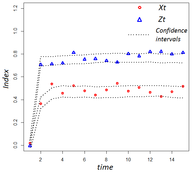
Figure 1: Toy model 26 : Sobol index estimate in function of time. Sample size: 200

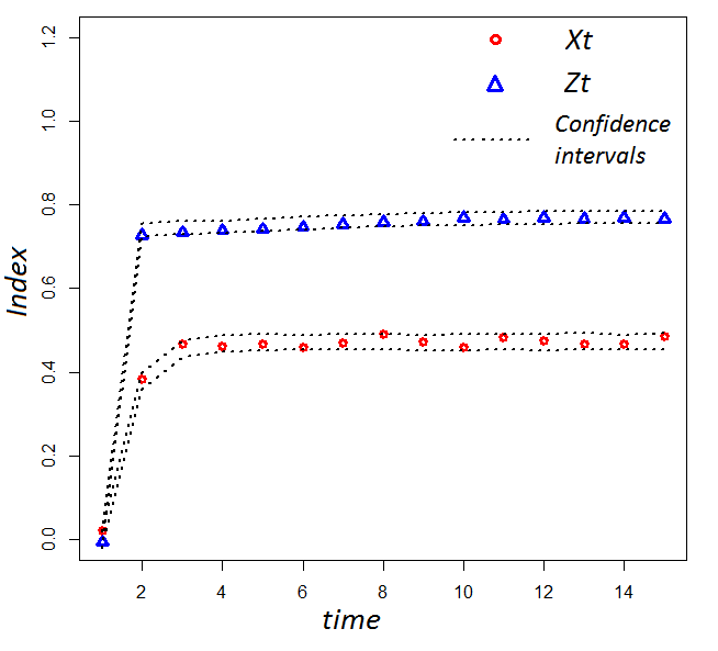
Figure 2: Toy model 26 : Sobol index estimate in function of time. Sample size: 10000

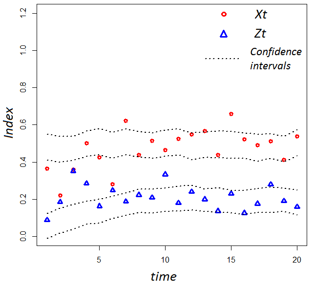
Figure 3: Toy model 27 : Sobol index estimate in function of time. Sample size: 200

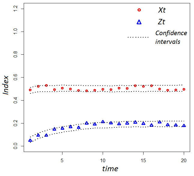
Figure 4: Toy model 27 : Sobol index estimate in function of time. Sample size: 10000

Figures 4, 4, 4, 4, display for each time step, $\displaystyle S_{t}^{X}=\frac{\mathbf{Var}(\mathbf{E}(Y_{t}|X_{\lfloor 0,t\rfloor}))}{\mathbf{Var}(Y_{t})}$, calculated for models (26) and (27) for different sizes of samples ($\displaystyle N=200$ and $\displaystyle N=10000$). Confidence intervals are stated at the 95% confidence level and plotted on each figures. The following examples exhibit two different types of convergence :

• the convergence of the estimator. At each time step, the Pick and Freeze algorithm estimates $\displaystyle S_{t}^{X}$. The quality of the estimator $\displaystyle\widehat{S}^{X}_{t}$ depends on the size of the sample. The confidence interval is smaller when $\displaystyle N=10000$. The convergence speed of the estimator is slow ($\displaystyle O(1/\sqrt{N})$) when we use a Monte Carlo sample. We could improve the speed using Quasi Monte Carlo (QMC) sample method [1]. But in our case QMC seems hard to implement.

• the temporal convergence : $\displaystyle\widehat{S}^{X}_{t}$ changes over time at each $\displaystyle t$. After just three iterations in time of the estimation algorithm, $\displaystyle S^{X}_{t}$ value reaches a limit (see on figures : 4 and 4). Model (26) is auto-regressive, it means that $\displaystyle Y_{t}$ depends on its past $\displaystyle Y_{t-1}$ and so, on all the past of $\displaystyle X_{t},Z_{t}$. We can rewrite it as :

  $$Y_{t}=\sum_{k=0}^{\infty}(0.2)^{k}(0.3X_{t-k}+Z_{t-k})$$

  At time $\displaystyle t=0$ for example, $\displaystyle S^{X}_{0}=\frac{\mathbf{Var}(\mathbf{E}(Y_{0}|X_{0}))}{\mathbf{Var}(Y_{0})}$. $\displaystyle Y_{0}$ is projected on a space of dimension 1 whereas it depends on $\displaystyle(X_{-\infty},\dots,X_{0},Z_{-\infty},\dots,Z_{0})$. The projection space is too small. When increasing this space, the index increases and converges to a constant. It’s what we call the phenomenon of memory which may refer to the physical concept of inertia. When $\displaystyle Y_{t}=\phi(X_{t},Z_{t})$ the index converges instantaneous (figures : 4, 4).

  The time convergence is interesting from a computing point of view. As the index converges to a constant, it useless to compute the index that takes into account the total trajectory of the process considered. It represents a lot of economy on a computational point of view because it requires less iterations for the evaluation of the index.

We can also notice that the method is independent of the expression of the model $\displaystyle f$. It is a black-box method requiring just the possibility to simulate a lot of inputs and outputs.

4 Application

4.1 The physical problem

We now address a model of building constructed as a metamodel [12] estimated thanks to observed data. This building is actually a classroom that welcomes students during the school year. It is therefore sensitive to hours, days but also holidays that occur during the year.

The studied room, whose internal temperature is $\displaystyle T^{\mathrm{int}}$ is surrounded by a corridor, an adjacent office, an office that is located below and a skylight (a shed). We have equipped these parts with temperature sensors. Temperatures are measured every hour denoted $\displaystyle(T^{\mathrm{below}},T^{\mathrm{above}},T^{\mathrm{off}},T^{\mathrm{cor}},T^{\mathrm{ext}},T^{\mathrm{int}})$. We also measure the temperature outside $\displaystyle T^{\mathrm{ext}}$. Obviously $\displaystyle T^{\mathrm{ext}}$ influences all the other temperatures $\displaystyle T^{\mathrm{below}},T^{\mathrm{above}},T^{\mathrm{off}},T^{\mathrm{cor}},T^{\mathrm{int}}$.

We choose to study the summer period when students are not present and when the heating is off.

4.2 The input and input-output models

We have to build a statistical input model and also an input-output model. After preprocessing inputs are modelled as a $\displaystyle VAR(p)$ process. Details are given in appendix B.

The output of the model is the internal temperature $\displaystyle T^{\mathrm{int}}$. Our sensitivity analysis aims to determine which among $\displaystyle T^{\mathrm{below}},T^{\mathrm{above}},T^{\mathrm{off}},T^{\mathrm{cor}},T^{\mathrm{ext}}$ impact the most the variance of the internal temperature $\displaystyle T^{\mathrm{int}}$. We choose to model the input-output system by a linear auto-regression of $\displaystyle T^{\mathrm{int}}$ on variables $\displaystyle U_{t}=(T^{e^{\prime}}_{t},T^{e^{\prime}}_{t-1})_{t}$, for $\displaystyle e^{\prime}\in\mathcal{E}^{\prime}=\{,\mathrm{below},\mathrm{above},\mathrm{off},\mathrm{cor},\mathrm{ext}\}$. The used model is given in appendix B. Note that if we have at our disposal a physical model able to simulate the input-output model (for instance an electrical model), we can use the data provided by this model to apply the Pick and Freeze method.

4.3 Numerical results

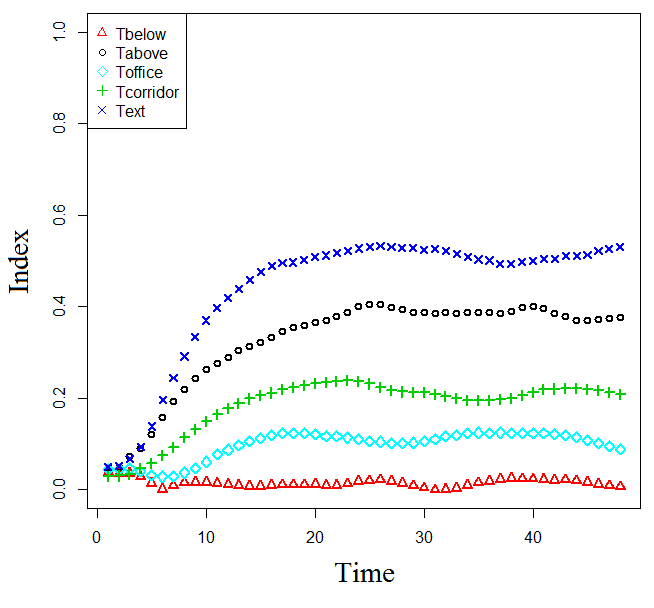
We then compute the different estimators $\displaystyle\widehat{S}^{X}_{t}=\widehat{S}^{e}_{t}$, for $\displaystyle t=2,\ldots,48$ and $\displaystyle e\in\mathcal{E}^{\prime}$. The results are gathered in figure : 5. Indices are estimated thanks to a sample of size $\displaystyle N=5000$.

Figure 5: Plots of estimated Sobol indices

The most influent variables are $\displaystyle T^{\mathrm{ext}}$ the external temperature and $\displaystyle T^{\mathrm{above}}$ the temperature of the room above. These two rooms have the most important noise variances : 1.34 and 0.62 (see $\displaystyle\Theta$ matrix (31)), whereas other noise variances are around 0.02. It seems logical that they are the most important variables in the sensitivity analysis. The number of time iterations is 20. The memory or inertia of the system is long enough.

Despite its small noise variance, $\displaystyle T^{\mathrm{cor}}$ is important. This variable illustrates the fact that sensitivity in a dependent context is not due only to the variance of the variable. Sensitivity is a function of the input-output relation and of the covariance between the variable of interest and the others. $\displaystyle T^{\mathrm{cor}}$ is the coldest room, it lowers the temperature $\displaystyle T^{\mathrm{int}}$. $\displaystyle T^{\mathrm{cor}}$ is most likely to cause temperature variations.

$\displaystyle T^{\mathrm{below}}$ is measured in a room located below the studied room $\displaystyle T^{\mathrm{int}}$ isolated by a slab. It seems logical that it does not affect $\displaystyle T^{\mathrm{int}}$.

Conclusion

In this article, we have proposed a modified definition of Sobol indices, adapted to dependent dynamic inputs. The index is no longer associated with the Hoeffding decomposition and the sum of the index is not equal to 1. Nevertheless, the index is between 0 and 1 and keeps the same interpretation. In a dynamic context the index varies with time but it is calculated as in a static case, that is to say that the input and the output are frozen at the same $\displaystyle t$ moment. With our proposition, we set in relief the dynamic aspect of the system by taking into account all the past of the input variables.

To estimate this index in the dependent framework we have chosen a Pick and Freeze method because it is flexible : it works whatever the nature of the input (dynamic or static) and whatever the number of inputs. The only problem is that it requires independent inputs. Yet, we can use this method even when the inputs are dependent and Gaussian because we can separate the inputs into two variables : one corresponding to the variable of interest (the one we need to study the sensitivity of the model) and another one which is totally independent. We can then apply the Pick and Freeze method on these new variables. We propose an algorithm to separate the variables and to calculate the index.

In the case of stationary variables this index approaches a limit quickly. On a computational perspective, this allows us to reduce the computation time, by only simulating the first instants of the process. This method requiring to calculate the inverse covariance matrix of the inputs, $\displaystyle VAR$ inputs have several advantages. Their covariance matrix can be calculated analytically and can be inversed easily thanks to their Toeplitz properties. These processes are quickly simulated; this is an advantage when we use the Pick and Freeze method which requires many input samples.

Appendix A Convergence of $\displaystyle S^{X}_{t}$ in the case where $\displaystyle Y_{t}=f_{t}(\mbox{\boldmath{$U$}}_{t},\dots,\mbox{\boldmath{$U$}}_{0})$

Assumption 2.

$\displaystyle(\mbox{\boldmath{$U$}}_{t})_{t\in\mathbb{Z}}$ is a causal regular linear process.

Causality means that $\displaystyle\mbox{\boldmath{$U$}}_{t}$ does not depend on a distant past. Formally if $\displaystyle H^{U}_{s}$ is the Hilbert space (for the covariance scalar product) generated by $\displaystyle\{\mbox{\boldmath{$U$}}_{v},v\leq s\}$ then $\displaystyle\underset{s\in\mathbb{Z}}{\cap}H_{s}^{U}=\{0\}$. Causality and linearity are equivalent to the existence of a representation :

$$\mbox{\boldmath{$\displaystyle U$}}_{t}=\sum_{k=0}^{\infty}C_{k}\mbox{\boldmath{$\displaystyle\omega$}}_{t-k}$$ (29)

where $\displaystyle\{\mbox{\boldmath{$\omega$}}_{t}\}$ is a vectorial white noise, $\displaystyle\mathbf{E}(\mbox{\boldmath{$\omega$}}_{t}\mbox{\boldmath{$\omega$}}^{*}_{t})=\Theta$ and $\displaystyle C_{k}$ are $\displaystyle(p\times p)$ matrices such that $\displaystyle\Sigma\|C_{k}\|^{2}<\infty$.

Basic examples are $\displaystyle VARMA$ processes associated to recurrence equations :

$$P(d)(\mbox{\boldmath{$U$}}_{t})=Q(d)(\mbox{\boldmath{$\omega$}}_{t})$$

where $\displaystyle d$ is the backward operator defined as $\displaystyle d(\mbox{\boldmath{$U$}}_{t})=\mbox{\boldmath{$U$}}_{t-1},d(\mbox{\boldmath{$\omega$}}_{t})=\mbox{\boldmath{$\omega$}}_{t-1}$ and $\displaystyle P,Q$ are polynomials such that $\displaystyle|P(z)|\neq 0$ for $\displaystyle|z|<1$ for stationarity and $\displaystyle|Q(z)|\neq 0$ for regularity ($\displaystyle H^{\omega}_{s}=H^{U}_{s}$ for every $\displaystyle-\infty<s<+\infty$).

We need the following truncation result. Let $\displaystyle\eta$ fixed. We can find $\displaystyle K$ such that :

$$\|\mbox{\boldmath{$U$}}_{t}-\mbox{\boldmath{$U$}}^{\tau(K)}_{t}\|\ <\eta$$

where $\displaystyle\mbox{\boldmath{$U$}}^{\tau(K)}_{t}=\sum_{k=t}^{t-K}C_{k}\mbox{\boldmath{$\omega$}}_{t-k}$

$$\mathbf{E}\left(|\sum_{k=t-K+1}^{\infty}C_{k}\mbox{\boldmath{$\omega$}}_{t-k}|\right)\leq\sum_{k=K+1}^{\infty}\|\Theta\|\|C_{k}\|^{2}$$

Assumption 3.

on the output

• $\displaystyle Y^{\star}_{t}$ has the denominated truncation property as $\displaystyle t\rightarrow\infty$ :

  $$\lim\limits_{t\to\infty}\mathbf{E}(|Y^{\star}_{t}-Y_{t}|^{2})=0$$

  and

  $$\lim\limits_{t\to\infty}|E(|Y^{\star}_{t}|^{2})-E(|Y_{t}|^{2})|=0$$

• $\displaystyle Y^{\star}_{t}$ has the conditional past truncation property as $\displaystyle t\rightarrow\infty$ :

  $$\lim\limits_{t\to\infty}\mathbf{E}(\mathbf{E}(Y^{\star}_{t}|X_{\lfloor-\infty,t\rfloor})^{2})-\mathbf{E}(\mathbf{E}(Y^{\star}_{t}|X_{\lfloor 0,t\rfloor})^{2})=0$$

From the Jensen inequality :

$$\mathbf{E}\left(\mathbf{E}(Y^{\star}_{t}|X_{\lfloor 0,t\rfloor})-\mathbf{E}(Y_{t}|X_{\lfloor 0,t\rfloor})\right)^{2}\leq\mathbf{E}(Y^{\star}_{t}-Y_{t})^{2}$$

tends to zero as $\displaystyle t\rightarrow\infty$

$\displaystyle\mathbf{E}\left(\mathbf{E}(Y^{\star}_{t}|X_{\lfloor-\infty,t\rfloor})^{2}\right)$ is constant by translation invariance and denoted $\displaystyle(S^{X}_{t})^{\star}.\mathbf{Var}(Y_{t})$.

From assumption 2 $\displaystyle\mathbf{E}(\mathbf{E}(Y^{\star}_{t}|X_{\lfloor 0,t\rfloor})^{2})\rightarrow(S^{X}_{t})^{\star}.\mathbf{Var}(Y_{t})$ as $\displaystyle t\rightarrow\infty$

By assumption 1 :

We can rewrite :

$$\mathbf{E}(Y_{t}|X_{\lfloor 0,t\rfloor})=\mathbf{E}(Y^{\star}_{t}|X_{\lfloor 0,t\rfloor})+\mathbf{E}(Y_{t}-Y^{\star}_{t}|X_{\lfloor 0,t\rfloor})$$

Then :

$$\mathbf{E}(\mathbf{E}(Y_{t}|X_{\lfloor 0,t\rfloor})^{2})=\mathbf{E}(\mathbf{E}(Y^{\star}_{t}|X_{\lfloor 0,t\rfloor})^{2})+\mathbf{E}(\mathbf{E}(Y_{t}-Y^{\star}_{t}|X_{\lfloor 0,t\rfloor})^{2})+2\mathbf{E}(\mathbf{E}(Y^{\star}_{t}|X_{\lfloor 0,t\rfloor})\mathbf{E}(Y_{t}-Y^{\star}_{t}|X_{\lfloor 0,t\rfloor}))$$

When $\displaystyle t$ tends to $\displaystyle+\infty$ :

$$\displaystyle\lim\limits_{t\to\infty}\mathbf{E}(\mathbf{E}(Y^{\star}_{t}|X_{\lfloor 0,t\rfloor})^{2})=(S^{X}_{t})^{\star}.\mathbf{Var}(Y_{t})$$

$$\displaystyle\lim\limits_{t\to\infty}\mathbf{E}(\mathbf{E}(Y_{t}-Y^{\star}_{t}|X_{\lfloor 0,t\rfloor})^{2})=0$$

$$\displaystyle\lim\limits_{t\to\infty}\mathbf{E}(\mathbf{E}(Y^{\star}_{t}|X_{\lfloor 0,t\rfloor})\mathbf{E}(Y_{t}-Y^{\star}_{t}|X_{\lfloor 0,t\rfloor}))=0\text{ from Schwartz ineguality}$$

So under the hypotheses 1 and 2 :

$$\lim\limits_{t\to\infty}S^{X}_{t}=(S^{X}_{t})^{\star}$$ (30)

Example :

Let us check assumptions 1 and 2 for the example :

$$Y_{t}^{\star}=\alpha Y_{t-1}^{\star}+B\mbox{\boldmath{$U$}}_{t}$$

for $\displaystyle\mbox{\boldmath{$U$}}_{t}$ causal regular Gaussian process and $\displaystyle|\alpha|<1$.
$\displaystyle Y_{t}$ can be written as :

$$Y_{t}^{\star}=\sum_{k=0}^{\infty}\alpha^{k}B\mbox{\boldmath{$U$}}_{t-k}$$

and

$$Y_{t}=\sum_{k=0}^{t}\alpha^{k}B\mbox{\boldmath{$U$}}_{t-k}$$

thus :

$$\mathbf{E}|Y_{t}^{\star}-Y_{t}|^{2}\leq C|\alpha|^{2t}$$

thus the assumption 1 is verify. Now we calculate :

$$\mathbf{E}(Y_{t}^{\star}|X_{\lfloor-\infty,t\rfloor})=\sum_{k=0}^{\infty}\alpha^{k}B\mathbf{E}(\mbox{\boldmath{$U$}}_{t-k}|X_{\lfloor-\infty,t\rfloor})$$

we know that

$$\mathbf{E}(\mbox{\boldmath{$U$}}_{t-k}|X_{\lfloor-\infty,t\rfloor})=\sum_{j=0}^{\infty}C_{j}\mathbf{E}(\omega_{t-j}|X_{\lfloor-\infty,t\rfloor})$$

and if $\displaystyle\eta$ given it exists $\displaystyle K$.
$\displaystyle\|U_{t-k}-U^{K}_{t-k}\|\leq\eta$ implies $\displaystyle\|\mathbf{E}(U_{t-k})-\mathbf{E}(U^{K}_{t-k})\|\leq\eta$ for $\displaystyle K$ large enough from the truncation property of causal processes. But from the regularity of $\displaystyle\mbox{\boldmath{$U$}}_{t}$ we have :$\displaystyle H^{X}_{u}=H^{\omega}_{u}$ for all $\displaystyle u$ thus in Gaussian case : $\displaystyle\mathbf{E}(\omega_{t-j}|X_{\lfloor-\infty,t\rfloor})=\mathbf{E}(\omega_{t-j}|\omega_{\lfloor-\infty,t\rfloor})$. But for $\displaystyle t-j>0$, $\displaystyle\omega_{t-j}$ is independent of $\displaystyle\{\omega_{s},s<0\}$.

Thus

$$\displaystyle\mathbf{E}(\omega_{t-j}|X_{\lfloor-\infty,t\rfloor}) \displaystyle=\mathbf{E}(\omega_{t-j}|\omega_{\lfloor-\infty,t\rfloor})$$

$$\displaystyle=\mathbf{E}(\omega_{t-j}|\omega_{\lfloor 0,t\rfloor})$$

$$\displaystyle=\mathbf{E}(\omega_{t-j}|X{\lfloor 0,t\rfloor})$$

and we have proved the result choosing $\displaystyle t$ large enough to have $\displaystyle t-K>0$.

Appendix B Construction of the statistical metamodel

To build a model easy to use for simulations, we need to preprocess the data in order to be placed in a stationary condition. We built a model for summers. $\displaystyle T^{e}_{t}$ is a scalar time series of input data. Preprocessing means first to transform $\displaystyle\bar{T}^{e}_{t}$ into $\displaystyle T^{e}_{t}$ :

$$\bar{T}^{e}_{t}=S(t)+V(t)*T^{e}_{t}\;\;\forall e\in\mathcal{E}$$

where $\displaystyle\mathcal{E}=\{\mathrm{int},\mathrm{ext},\mathrm{above},\mathrm{below},\mathrm{cor},\mathrm{off}\}$, $\displaystyle S(t)$ is the mean with period 24 hours, $\displaystyle V(t)$ the variance periodic function and $\displaystyle T^{e}_{t}$ a stationary or cyclo-stationary process.

Temperatures ($\displaystyle T^{\mathrm{below}},T^{\mathrm{above}},T^{\mathrm{off}},T^{\mathrm{cor}},T^{\mathrm{ext}},T^{\mathrm{int}}$) are modelled by a $\displaystyle VAR$ process for working days:

$$\forall e\in\mathcal{E},\;\;T_{t}^{e}=\sum_{f\in\mathcal{E}}\gamma_{f}^{e}T_{t-1}^{f}+\omega_{t}^{e},$$

where $\displaystyle(\omega_{t}^{e})_{t\in\mathbb{N},e\in\mathcal{E}}$ are Gaussian variables with covariance $\displaystyle\Theta$. Let $\displaystyle\mbox{\boldmath{$T$}}_{t}=(T^{e}_{t})_{e\in\mathcal{E}},\;\;\mbox{\boldmath{$\omega$}}_{t}=(\omega_{t}^{e})_{e\in\mathcal{E}}$ thus :

$$\mbox{\boldmath{$T$}}_{t}=\sum_{l=1}^{p}D_{l}\mbox{\boldmath{$T$}}_{t-p}+\mbox{\boldmath{$\omega$}}_{t}$$

For every fixed $\displaystyle p$ we estimated $\displaystyle(D_{l},\;\;l\leq 1,\dots,p)$ and $\displaystyle\Theta$ the covariance of $\omega$ by maximum of likelihood under the constraint imposed by the stationarity of $\displaystyle\mbox{\boldmath{$T$}}_{t}$. Then we choose $\displaystyle p$ using AIC criteria; obtaining $\displaystyle p=2$.

$\displaystyle D_{1}$ and $\displaystyle D_{2}$ estimated are :

$$\begin{array}[]{c c}D_{1}=\begin{pmatrix}0.88&0.01&0.06&0.06&0\\ -0.23&1.21&0.01&0.49&0.3\\ 0.21&0.03&1.24&0.06&0.01\\ 0.12&0.06&0.03&1&0.01\\ 0.20&0.61&-0.19&0.71&0.85\end{pmatrix}&D_{2}=\begin{pmatrix}0.04&-0.01&-0.07&-0.04&0.01\\ 0.03&-0.48&-0.04&-0.08&-0.04\\ -0.16&-0.02&-0.30&-0.09&-0.10\\ -0.03&-0.04&-0.05&-0.15&-0.01\\ -0.45&-0.60&0.25&-0.31&-0.05\end{pmatrix}\end{array}$$

The $\displaystyle\Theta$ matrix estimated is :

$$\Theta=\begin{array}[]{l}T^{\mathrm{below}}\\ T^{\mathrm{above}}\\ T^{\mathrm{off}}\\ T^{\mathrm{cor}}\\ Text\end{array}\begin{pmatrix}0.01&0.01&0.004&0.01&0.01\\ 0.01&0.62&0.02&0.03&0.46\\ 0.004&0.02&0.03&0.002&0.04\\ 0.01&0.03&0.002&0.02&0.04\\ 0.01&0.46&0.04&0.04&1.34\end{pmatrix}$$ (31)

The input-output system is modelled by an auto-regression of $\displaystyle T^{\mathrm{int}}$ on variables
$\displaystyle\mbox{\boldmath{$U$}}_{t}=(T^{\mathrm{below}},T^{\mathrm{above}},T^{\mathrm{off}},T^{\mathrm{cor}},T^{\mathrm{ext}})$ :

$$\forall t\geq 1,\;\;T^{\mathrm{int}}(t)=\sum_{e\in\mathcal{E},k=1}^{2}\phi_{e,k}T_{e,t-k}+\sum_{k=1}^{2}\phi_{int,k}T^{\mathrm{int}}_{t-k}$$ (32)

where $\displaystyle\mathcal{E}=\{\mathrm{int},\mathrm{above},\mathrm{below},\mathrm{cor},\mathrm{off},\mathrm{ext},\}$

References

• [1] Andrea Saltelli, Karen Chan, E Marian Scott, et al. Sensitivity analysis, volume 1. Wiley New York, 2000.
• [2] Ruixue Liu and Art B Owen. Estimating mean dimensionality of analysis of variance decompositions. Journal of the American Statistical Association, 101(474):712–721, 2006.
• [3] Il’ya M. Sobol. Sensitivity estimates for nonlinear mathematical models. Math. Modeling Comput. Experiment, 1(4):407–414 (1995), 1993.
• [4] Il’ya M. Sobol. Global sensitivity indices for nonlinear mathematical models and their Monte Carlo estimates. Mathematics and Computers in Simulation, 55(1-3):271–280, 2001.
• [5] Thierry A Mara and Stefano Tarantola. Variance-based sensitivity indices for models with dependent inputs. Reliability Engineering & System Safety, 2011.
• [6] Sergei Kucherenko, Stefano Tarantola, and Paola Annoni. Estimation of global sensitivity indices for models with dependent variables. Computer Physics Communications, 183(4):937–946, 2012.
• [7] Gaëlle Chastaing, Fabrice Gamboa, and Clémentine Prieur. Generalized hoeffding-sobol decomposition for dependent variables-application to sensitivity analysis. Electronic Journal of Statistics, 6:2420–2448, 2012.
• [8] Fabrice Gamboa, Alexandre Janon, Thierry Klein, Agnes Lagnoux-Renaudie, and Clémentine Prieur. Statistical inference for sobol pick freeze monte carlo method. arXiv preprint arXiv:1303.6447, 2013.
• [9] G. Chastaing, F. Gamboa, and C. Prieur. Generalized hoeffding-sobol decomposition for dependent variables-application to sensitivity analysis. Arxiv preprint arXiv:1112.1788, 2011.
• [10] Alexandre Janon, Thierry Klein, Agnès Lagnoux, Maëlle Nodet, and Clémentine Prieur. Asymptotic normality and efficiency of two sobol index estimators. Preprint available at http://hal.inria.fr/hal-00665048/en, 2012.
• [11] Peter J. Brockwell and Richard A. Davis. Time Series: Theory and Methods. Springer, 2nd ed. 1991. 2nd printing 2009 edition, April 2009.
• [12] Robert Faivre, Bertrand Iooss, Stéphanie Mahévas, David Makowski, and Hervé Monod. Analyse de sensibilité et exploration de modèles: Application aux sciences de la nature et de l’environnement. Editions Quae, 2013.