Topics in Two-Loop Superstring Perturbation Theory

Abstract.

In this contribution to the Proceedings of the Conference on Analysis, Complex Geometry, and Mathematical Physics, an expository overview of superstring perturbation theory to two loop order is presented to an audience of mathematicians and physicists. Recent results on perturbative supersymmetry breaking effects in Heterotic string theory compactified on ${\mathbb{Z}}_{2}\times{\mathbb{Z}}_{2}$ Calabi-Yau orbifolds, and the calculation of the two-loop vacuum energy in these theories are discussed in detail, and the appearance of a new modular identity with respect to $Sp(4,{\mathbb{Z}})/{\mathbb{Z}}_{4}$ is reviewed.

1. Introduction

Superstring theory is understood most precisely in two limits. The first is the long-distance limit (equivalently referred to as the low energy limit) in which the theory is probed at length scales much larger than the characteristic string length. To leading order in this limit, superstring theory reduces to supergravity, which is a supersymmetric extension of Einstein’s general relativity. The second limit is for weakly interacting strings in which the theory is expanded in powers of the string coupling. This asymptotic expansion is referred to as superstring perturbation theory. The two limits are complementary in the sense that the string coupling may be large in the supergravity limit, while the distance scales probed may be comparable to the string length in superstring perturbation theory.

The physical motivation for superstring theory stems from the fact that it inevitably unifies Yang-Mills theory, general relativity, and supersymmetry in a consistent quantum mechanical framework. As a generalization of quantum field theory, superstring theory is expected to provide insights into particle physics beyond the Standard Model. As a quantum theory of gravity, superstring theory is expected to shed light on the physics of black holes and the early universe. A recent historical overview of the development of string theory may be found in [C].

The mathematical interest in superstring theory and quantum field theory derives from their deep connections with a wide range of subjects in differential and algebraic geometry. Several of these connections were reviewed and explained in the volumes Quantum Fields and Strings: A course for Mathematicians in [D].

In the present paper, we shall concentrate on the mathematical and physical aspects of string perturbation theory, which may be formulated in terms of a statistical summation over randomly fluctuating two-dimensional surfaces of arbitrary topology. The basic mathematical objects of interest are conformal field theories on compact Riemann surfaces, and the moduli spaces of these Riemann surfaces for arbitrary genus. In physics, the genus is referred to as the number of loops. The presence of fermions in superstring perturbation theory requires compact super Riemann surfaces and their super moduli spaces. For contributions of genus 0 and 1 the distinction between Riemann surfaces and super Riemann surfaces, and between moduli space and super moduli space in string perturbation theory is immaterial. The true novelty of dealing with the moduli space of super Riemann surfaces first appears at genus 2. It is largely for this reason that Phong and I have concentrated on the study of two loop superstrings for over a decade.

The goal of this paper is to present an overview of the main results on two-loop superstring perturbation theory, and their applications. Many of these results have originally been obtained in relatively lengthy and technical papers, and so we shall take this opportunity to provide a guide through the literature on this subject.

The remainder of this paper is organized as follows. In the first half, we shall present a brief introduction to superstring perturbation theory and its relation with super Riemann surfaces and their moduli spaces. A review of early work on the subject may be found in [DP1], while an extensive modern treatment is provided in [W2]. Lecture notes on the subject, destined for an audience of Mathematicians, may be found in the author’s contribution to the volumes of [D].

The geometry of the genus 2 super moduli space, and its applications to the construction of selected superstring quantum amplitudes in terms of modular forms and Jacobi $\vartheta$-functions is discussed next. An early overview of results prior to 2002 may be found in [DP8]; references to more recent results will be pointed out in the body of the paper. A variety of applications of the formula for the genus 2 amplitude with four massless external states will be discussed. We shall briefly comment on some of the issues involved in the construction of higher loop amplitudes. Finally, in the second half of the paper, we shall review recent results on perturbative supersymmetry breaking in Heterotic string theories compactified on ${\mathbb{Z}}_{2}\times{\mathbb{Z}}_{2}$ Calabi-Yau orbifolds, the calculation of the corresponding two-loop vacuum energy in these models, and their mathematical underpinning involving the Deligne-Mumford compactification divisors of super moduli space.

Acknowledgments

First and foremost, I wish to express my deep gratitude to my long-time friend D.H. Phong for the rewarding collaboration that began 30 years and 50 publications ago. In particular, the research reported on in this article has been carried out jointly with him.

Throughout our work on two-loop superstring perturbation theory, we have greatly benefited from correspondence with Edward Witten. I would like to acknowledge the organizers, Paul Feehan, Jian Song, Ben Weinkove, and Richard Wentworth for putting together a splendid conference and celebration in honor of D.H. Phong.

Finally, I would like to thank the Kavli Institute for Theoretical Physics at the University of California, Santa Barbara for their hospitality and the Simons Foundation for their support while this work was being completed. This research was supported in part by the National Science Foundation under grants PHY-07-57702, PHY-11-25915, and PHY-13-13986.

2. String Perturbation Theory

Strings are 1-dimensional objects, whose characteristic size is set by the Planck length $\ell_{P}\sim 10^{-35}\,m$, a scale which is $10^{19}$ times smaller than the size of a proton. A string may be open with the topology of a line interval, or closed with the topology of a circle. It lives in a space-time $M$, which is usually a manifold or an orbifold, whose dimension is denoted by $d$. Phyisical space-time has dimension 4, but consistent string theories will require $d=10$. As a string evolves in time, it sweeps out a 2-dimensional surface in $M$, which may be described by a map $x$ from a reference 2-dimensional surface, or worldsheet, $\Sigma$ into $M$ (see Figure 1). The surface $\Sigma$ carries a metric $g$, and the space-time $M$ carries a metric $G$ which is independent of $g$. We shall restrict to theories of orientable strings for which $\Sigma$ is orientable and thus a Riemann surface. Four out of the five known string theories, namely Type IIA and Type IIB and the Heterotic string theories with gauge groups $Spin(32)/{\mathbb{Z}}_{2}$ and $E_{8}\times E_{8}$ are all based on orientable strings.

Quantum strings require summing over all possible Riemann surfaces $\Sigma$, which includes summing over topologies of $\Sigma$, metrics $g$ on $\Sigma$, and maps $x:\Sigma\to M$. Therefore, the quantum string problem is essentially equivalent to the problem of fluctuating or random surfaces of arbitrary genus.

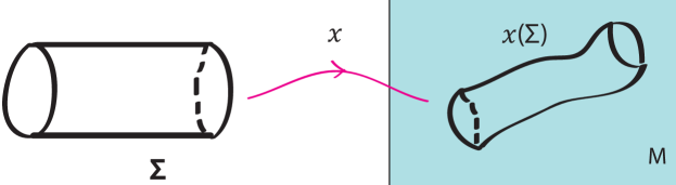
Figure 1. The map $x$ of $\Sigma$ into space-time $M$ for a closed string.

Of fundamental physical interest are the quantum amplitudes associated with scattering processes such as, for example, for two incoming strings scattering into two outgoing strings. The surface $\Sigma$ will then possess punctures at which vertex operators are inserted. The number of punctures is fixed for a given physical process, and the vertex operators encode the physical data of the incoming and the outgoing physical states, such as their space-time momentum, and their polarization vector (for Yang-Mills states) or polarization tensor (for gravitons).

Given the number of punctures, the remaining topological information of $\Sigma$ is its genus $h$. The summation over all $\Sigma$, required by quantum mechanics, includes a summation over all genera $h\in{\mathbb{N}}$. The contribution of genus $h$ is accompanied by a weight factor $(g_{s})^{2h-2}$ governed by the string coupling $g_{s}$ (see Figure 2.) This expansion in power of $g_{s}$ is referred to as string perturbation theory. Just as in quantum field theory, the perturbative expansion is asymptotic instead of convergent. The coefficient of order $h$ in the expansion is referred to as the $h$-loop contribution, and is itself given by an integral over all the fields that specify the strings, including all maps $x:\Sigma\to M$ and all metrics $g$ on $\Sigma$, with a weight factor $e^{-I}$ specified by the worldsheet action $I$. The space-time $M$ and its metric $G$ are considered fixed.

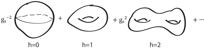
Figure 2. String perturbation expansion in powers of $g_{s}$.

For bosonic string theory, the maps $x$ and the metrics $g$ exhaust all the data of the quantum string, and the action $I$ is essentially the area of $x(\Sigma)$ induced by the metric $G$. The set-up is invariant under Diff$(\Sigma)$ and thus intrinsic. In its critical dimension $d=26$ the quantum theory of bosonic strings is further invariant under Weyl transformations of the metric $g$ on $\Sigma$. The integral over metrics $g$ then reduces to an integral over conformal classes $[g]$, or equivalently, over the moduli space ${\mathcal{M}}_{h}$ of Riemann surfaces of genus $h$, whose complex dimension is given by,

(2.1) $$\dim_{\mathbb{C}}({\mathcal{M}}_{h})=\left\{\begin{matrix}0&h=0&\cr 1&h=1&\cr 3h-3&h\geq 2\end{matrix}\right.$$

With $n$ additional punctures the dimension of moduli space is increased by $n$ for $h\geq 2$, by $n-1$ for $h=0$, and by $n-3$ for $h=0$. The bosonic theory in flat space-time $M={\mathbb{R}}^{26}$ turns out to be physically inconsistent, as it necessarily contains a tachyon, namely a particle that must always travel faster than the speed of light.

3. Superstrings

Physically relevant quantum string theories require the presence of fermionic degrees of freedom. Indeed, almost all the matter in Nature appears to be built on fermionic elementary constituents, such as electrons, protons, neutrons and, at a shorter length scale, quarks. Moreover, as was already pointed out, string theories with only bosonic degrees of freedom are inconsistent, at least in flat space-time.

The inclusion of fermionic degrees of freedom in strings is delicate, and results in far reaching alterations to the theory. Physical fermions correspond to spinors in space-time $M$, so their presence requires $M$ to be a spin manifold. Fermions then correspond to states which transform as spinors under the tangent group $SO(d-1,1)$ of $M$. The avenue followed most frequently in string theory is the so-called Ramond-Neveu-Schwarz (RNS) formulation, where all the field operators on $\Sigma$ are vectors under $SO(d-1,1)$, but the string spectrum has two distinct sectors. The NS sector consists of space-time bosons, built by applying the vector operators to a scalar ground state, while the R sector consists of space-time fermions, built by applying the vector operators to a spinor ground state. Consistency of the theory requires $d=10$ and truncation of the spectrum to a sector with space-time supersymmetry, which is referred to as the Gliozzi-Scherk-Olive (GSO) projection.

In the RNS formulation of the superstring, the Riemann surface is replaced with a super Riemann surface $\Sigma$. We shall often characterize the data on $\Sigma$ in terms of data on its underlying (or reduced) Riemann surface $\Sigma_{\rm red}$. On the super Riemann surface, the metric $g$ is extended to a pair $(g,\chi)$ where $\chi$ is a spinor, specifically a section of the line bundle $\bar{K}\otimes K^{-{1\over 2}}$, where $K$ is the canonical bundle of $\Sigma_{\rm red}$. Taking the square root of $K$ requires the assignment of a spin structure, which we denote by $\delta$. The map $x$ is extended to a pair $(x,\psi)$ where $\psi$ is a section of $K^{1\over 2}$ with values in ${\mathbb{R}}^{10}$, or more generally in the cotangent bundle $T^{*}(M)$. A more detailed description of $\chi$ and $\psi$ will be given in the section below; it will depend on the precise superstring theory under consideration. Finally, the action $I$ is extended to including the fields $\chi$ and $\psi$ and to being invariant under local supersymmetry transformations, in addition to diffeomorphisms Diff$(\Sigma)$.

Quantum superstring amplitudes are obtained by summing over all topologies of $\Sigma$, integrating over all $(g,\chi)$, as well as over all maps $(x,\psi)$. The integration over all $\chi$ and $\psi$ will be accompanied by a summation over spin structures $\delta$. This procedure will naturally implement the GSO projection, discussed earlier, in terms of the worldsheet data. In its critical dimension $d=10$ the quantum superstring is further invariant under superconformal transformations on $\Sigma$. As a result, the integration over $(g,\chi)$ at genus $h$ reduces to an integration over superconformal classes $[g,\chi]$, or equivalently over the moduli space $\mathfrak{M}_{h}$ of super Riemann surfaces. The dimension of the moduli space $\mathfrak{M}_{h}$ is finite and given as follows,

(3.1) $$\dim(\mathfrak{M}_{h})=\left\{\begin{matrix}(0|0)&h=0&\cr(1|0)&h=1&\delta~{}\hbox{even}\cr(1|1)&h=1&\delta~{}\hbox{odd}\cr(3h-3|2h-2)&h\geq 2\end{matrix}\right.$$

More precisely, super moduli space $\mathfrak{M}_{h}$ consists of two connected components $\mathfrak{M}_{h,+}$ and $\mathfrak{M}_{h,-}$, corresponding to even or odd spin structure assignments, and each moduli space includes strata for all spin structures with the corresponding parity. With $n$ additional punctures of the NS type (punctures of the type R will not be considered here), the dimension of super moduli space is increased by $(n|n)$ for $h\geq 2$, by $(n-1|n-1)$ for $h=1$, and by $(n-3|n-2)$ for $h=0$.

Clearly, one key alteration in passing from bosonic strings to superstrings is replacing the moduli space of Riemann surfaces by that for super Riemann surfaces. Actually, for genus 0, as well as for genus one and $\delta$ even, the two moduli spaces coincide in the absence of punctures, and no odd moduli are present. Furthermore, the odd modulus which appears at genus one for odd spin structure, and the odd moduli associated with the NS punctures for genus zero and one, merely plays the role of a book keeping device, and leave no geometrical imprint on the theory.

Thus, the full geometrical effect due to the presence of odd moduli will be felt starting only at two loops. Fortunately, every genus 2 Riemann surface is hyperelliptic, a fact that allows for many conceptual and practical simplifications. In particular, the super moduli space at genus 2 will enjoy special properties, not shared by its higher genus counterparts, as will be reviewed in section 6.

4. Independence of left and right chiralities

We shall now give a more detailed account of the structure of the map $(x,\psi)$, introduced in the previous section. In particular, we shall explain the chirality properties of $\psi$ that lead to the distinction between the four different closed orientable superstring theories. For simplicity, we shall take $M={\mathbb{R}}^{10}$, and choose local super conformal coordinates $(z,\theta)$ on $\Sigma$, in terms of which the map $(x,\psi)$ may be expressed in local coordinates on $M$ and $\Sigma$ by functions $x^{\mu}(z,\bar{z})$ and $\psi^{\mu}(z,\bar{z})$ with $\mu\in\{0,1,2,\cdots,9\}$. A natural starting point is to take each $\psi^{\mu}$ to be a reducible spinor with irreducible components $\psi_{+}^{\mu}$ and $\psi_{-}^{\mu}$ where $\psi_{+}$ is a section of $K^{1\over 2}$ and $\psi_{-}$ a section of its complex conjugate $\bar{K}^{1\over 2}$ both with values in ${\mathbb{R}}^{10}$. The assignments $\pm$ refer to left $(+)$ and right $(-)$ chiralities on $\Sigma$. The local equations satisfied by $(x,\psi)$, and their local solutions, are given by,

$$\partial_{z}\partial_{\bar{z}}x^{\mu}=0\hskip 18.06749pt x^{\mu}=x^{\mu}_{+}(z)+x^{\mu}_{-}(\bar{z})$$

(4.1) $$\partial_{\bar{z}}\psi_{+}^{\mu}=\partial_{z}\psi^{\mu}_{-}=0 \psi^{\mu}=(\psi_{+}^{\mu}(z),\,\psi_{-}(\bar{z}))$$

While the reality of the map $x$ requires the fields $x_{+}^{\mu}$ and $x_{-}^{\mu}$ to be complex conjugates of one another, the fields $\psi_{+}^{\mu}$ and $\psi_{-}^{\mu}$ should be viewed as independent of one another. The physical reason underlying this independence may be traced back to the fact that the Riemann surface $\Sigma$ really is an analytic continuation of a worldsheet whose metric has Minkowski $(-+)$ signature, and whose left and right chirality Weyl spinors are independent left and right Majorana-Weyl spinors. This is unlike when the worldsheet has Euclidean $(++)$ signature and the two Weyl spinors are necessarily complex conjugates of one another. The field $\chi$ similarly decomposes into independent spinors $\chi=(\chi^{+},\chi^{-})$ whose spin structure assignments are independent.

In the critical space-time dimension $d=10$, there are five fundamental consistent superstrings theories. One of these, namely the Type I superstring theory, contains both open and closed strings, and requires the inclusion of unorientable worldsheets. The four closed orientable superstring theories are as follows.

$\bullet$ Type II superstrings
For Type II superstrings, the fields $\psi^{\mu}_{+}$ are sections of $K^{1\over 2}$ and $\chi^{+}$ is a section of $\bar{K}\otimes K^{-{1\over 2}}$, both with spin structure $\delta=\delta_{L}$. The field $\psi^{\mu}_{-}$ is a section of $\bar{K}^{1\over 2}$ and $\chi^{-}$ is a section of $K\otimes\bar{K}^{-{1\over 2}}$, both with spin structure $\delta_{R}$. We stress that the fields $\psi$ and $\chi$ for opposite chiralities, as well as their spin structures $\delta_{L}$ and $\delta_{R}$, are independent of one another. The distinction between Type IIA and Type IIB is made on the basis of the chirality of the gravitino particles (the superpartners of the graviton), or equivalently, between the parity of the contributions of even and odd spin structures on the worldsheet. Type II theories were discovered, and their tree-level and one-loop 4-point amplitudes were computed in [GS].

$\bullet$ Heterotic superstrings
For the Heterotic strings, we have $\chi^{-}=0$, and we retain only $\chi^{+}$. Note that the independence of both chiralities is essential to achieve this. Thus, the moduli space associated with $+$ chirality is that of super Riemann surfaces, while the one associated with $-$ chirality is the moduli space of ordinary Riemann surfaces. To complete the theory, 32 fermionic fields of right chirality $\psi^{A}_{-}(\bar{z})$ with $A\in\{1,2,\cdots,32\}$ are included, but we stress that there is no corresponding $\chi^{-}$. The spin structure assignments distinguish the two Heterotic strings. For $Spin(32)/{\mathbb{Z}}_{2}$, the spin structure of $\psi_{-}^{A}(\bar{z})$ is the same $\delta_{R}$ for all values of $A$. For $E_{8}\times E_{8}$, the spin structure for $1\leq A\leq 16$ is $\delta_{R1}$, while the spin structure for $17\leq A\leq 32$ is $\delta_{R2}$ and is independent of $\delta_{R1}$. Heterotic theories were discovered, and their tree-level and one-loop 4-point amplitudes were computed in [GHMR].

5. Matching left and right moduli spaces

Since the fermionic degrees of freedom of left and right chirality are independent of one another, so should the odd part of moduli space be. This independence is most striking in the case of the Heterotic string, where left chirality odd moduli are present, but no right chirality odd moduli exist. As the contributions of left and right chiralities are assembled to produce physical string amplitudes, one must impose a prescription which is consistent with the symmetries of the amplitudes (barring known anomalies), and gauge fixing. The super period matrix provides the basic tool for genus 2, as will be discussed in detail in the subsequent section [DP8]. For arbitrary genus, a general prescription was provided in [W2], which adds further precision also to the case of genus two, and which we summarize next.

To left chirality, one associates a super moduli space $\mathfrak{M}_{hL}$, which has dimension $(3h-3|2h-2)$, and on which one introduces local superconformal coordinates $(m_{L},\bar{m}_{L};\zeta_{L})$. Here, $\bar{m}_{L}$ is the complex conjugate of $m_{L}$. The odd moduli $\zeta_{L}$ are complex, but there is no concept of their complex conjugates.

To right chirality, for Type II, one associates a super moduli space $\mathfrak{M}_{hR}$ of dimension $(3h-3|2h-2)$ which is independent of $\mathfrak{M}_{hL}$, and for which one introduces local superconformal coordinates $(m_{R},\bar{m}_{R};\zeta_{R})$. To right chirality, for Heterotic, one associates a purely even moduli space ${\mathcal{M}}_{h}$ of dimension $(3h-3|0)$, with local complex coordinates $(m_{R},\bar{m}_{R})$. Again, $\bar{m}_{R}$ is the complex conjugate of $m_{R}$.

Assembling left and right chiralities, odd moduli will remain independent, but even moduli must be related by a procedure which, in the absence of odd moduli, reduces to complex conjugation. For the Heterotic case, one might be tempted to set $\bar{m}_{R}=m_{L}$, but this choice is inconsistent with the requirement of gauge slice-independence. This identification would amount to carrying out a projection $\mathfrak{M}_{h}\to{\mathcal{M}}_{h}$, which is known to not exists globally for sufficiently high genus [DW].

The prescription given in [W2] for the Heterotic string is to integrate over a closed cycle $\Gamma\subset\mathfrak{M}_{hL}\times{\mathcal{M}}_{h}$ of complex bosonic dimension $3h-3$ and odd dimension $2h-2$. The cycle $\Gamma$ is required to be such that $\bar{m}_{R}=m_{L}+$ nilpotent corrections which vanish when $\zeta_{L}=0$. It is also subject to certain matching conditions along the Deligne-Mumford compactification divisors of $\mathfrak{M}_{hL}$ and ${\mathcal{M}}_{h}$. BRST symmetry of the integrand and a superspace version of Stokes’s theorem guarantee independence of the integral on the choice of closed cycle $\Gamma$.

6. The super period matrix at genus 2

The super period matrix was introduced in [DP1], and its properties were studied systematically in [DP3] for both even and odd spin structures. A formal approach based more on algebraic geometry may be found in [RSV]. For genus two, the super period matrix provides a natural projection of the moduli space of super Riemann surfaces $\mathfrak{M}_{2}$ onto the moduli space of Riemann surfaces ${\mathcal{M}}_{2}$, specifically onto its spin moduli space ${\mathcal{M}}_{2,{\rm spin}}$ for even spin structures [DP2, W1].

To define the super period matrix, we fix a canonical basis of cycles $\mathfrak{A}_{I}$ and $\mathfrak{B}_{I}$ for $H^{1}(\Sigma,{\mathbb{Z}})$ with intersections $\#(\mathfrak{A}_{I},\mathfrak{A}_{J})=\#(\mathfrak{B}_{I},\mathfrak{B}_{J})=0$ and $\#(\mathfrak{A}_{I},\mathfrak{B}_{J})=\delta_{IJ}$ for $I,J\in\{1,2\}$. Introducing a dual basis of holomorphic 1-forms $\omega_{I}$, which are canonically normalized on $\mathfrak{A}$-cycles, the ordinary period matrix $\Omega_{IJ}$ is defined by,

(6.1) $$\oint_{\mathfrak{A}_{I}}\omega_{J}=\delta_{IJ}\hskip 72.26999pt\oint_{\mathfrak{B}_{I}}\omega_{J}=\Omega_{IJ}$$

The period matrix is symmetric and, up to identifications under the modular group, its 3 independent complex entries provide complex coordinates for ${\mathcal{M}}_{2}$. On a super Riemann surface with even spin structure there exist two super holomorphic 1/2 forms $\hat{\omega}_{I}$ satisfying ${\mathcal{D}}_{-}\hat{\omega}_{I}=0$ which may again be canonically normalized on $\mathfrak{A}$-periods. The super period matrix $\hat{\Omega}_{IJ}$ is defined by,

(6.2) $$\oint_{\mathfrak{A}_{I}}\hat{\omega}_{J}=\delta_{IJ}\hskip 72.26999pt\oint_{\mathfrak{B}_{I}}\hat{\omega}_{J}=\hat{\Omega}_{IJ}$$

The relation between the super period matrix $\hat{\Omega}_{IJ}$ and the period matrix $\Omega_{IJ}$ may be exhibited concretely. We use local complex coordinates $(z,\bar{z})$ corresponding to the complex structure imposed by $\Omega_{IJ}$, and denote by $S[\delta](z,w)=S[\delta](z,w;\Omega)$ the Szego kernel for spin structure $\delta$, whose pole at $z=w$ is normalized to unit residue. The super period matrix is then given by,

(6.3) $$\qquad\hat{\Omega}_{IJ}=\Omega_{IJ}-{i\over 8\pi}\int_{\Sigma}\int_{\Sigma}\omega_{I}(z)\chi(z)S[\delta](z,w;\Omega)\chi(w)\omega_{J}(w)$$

The super period matrix is symmetric $\hat{\Omega}_{JI}=\hat{\Omega}_{IJ}$, and its imaginary part is positive. It is invariant under changes of slice $\chi$, performed with the help of local supersymmetry transformations. Thus, every period matrix $\hat{\Omega}_{IJ}$ at genus 2 corresponds to an ordinary Riemann surface, with spin structure $\delta$, modulo the action of the modular group $Sp(4,{\mathbb{Z}})$. As a result, for even spin structures, the super period matrix provides a projection of $\mathfrak{M}_{2}$ onto ${\mathcal{M}}_{2,{\rm spin}}$ which is natural and smooth.

7. The chiral measure in terms of $\vartheta$-functions

The procedure for obtaining the genus 2 chiral measure using the projection provided by the super period matrix was introduced in [DP5]. The super period matrix provides a natural set of coordinates on $\mathfrak{M}_{2}$ given by,

(7.1) $$m^{A}=(\hat{\Omega}_{IJ},\zeta^{\alpha})\hskip 72.26999pt\alpha\in\{1,2\}$$

Using local supersymmetry transformations, the following gauge is chosen for $\chi$,

(7.2) $$\chi(z)=\zeta^{1}\delta(z,q_{1})+\zeta^{2}\delta(z,q_{2})$$

where $q_{\alpha}$ are two arbitrary points on $\Sigma_{\rm red}$. To formulate the superstring amplitudes in terms of $\hat{\Omega}$ rather than $\Omega$, we perform a deformation of complex structures by a Beltrami differential $\hat{\mu}$. Under this deformation, we have,

(7.3) $$\Omega\to\hat{\Omega}\hskip 21.68121pt\left\{\begin{matrix}g&\to&\hat{g}=g+\hat{\mu}\cr\bar{\partial}&\to&\bar{\partial}+\hat{\mu}\,\partial\cr\langle{\mathcal{O}}\rangle(g)&\to&\langle{\mathcal{O}}\rangle(\hat{g})+\int\hat{\mu}(z)\langle T(z){\mathcal{O}}\rangle\end{matrix}\right.$$

where $\langle{\mathcal{O}}\rangle(g)$ stands for the expectation value of any operator ${\mathcal{O}}$ in the quantum field theory on the surface $\Sigma$ with metric $g$, and $T(z)$ stands for the stress tensor. Local supersymmetry invariance guarantees that any physical superstring amplitude will be independent of the points $q_{\alpha}$.

The evaluation of the genus 2 superstring chiral measure on $\mathfrak{M}_{2}$, following the procedure outlined above, is quite involved [DP6] but the final result is remarkably simple when expressed in terms of the super period matrix. For a flat Minkowski space-time manifold $M={\mathbb{R}}^{10}$, one finds [DP7, DP8],

(7.4) $$\qquad d\mu[\delta](\hat{\Omega},\zeta)=\left({\mathcal{Z}}[\delta](\hat{\Omega})+\zeta^{1}\zeta^{2}{\vartheta[\delta](0,\hat{\Omega})^{4}\,\Xi_{6}[\delta](\hat{\Omega})\over 16\pi^{6}\,\Psi_{10}(\hat{\Omega})}\right)d^{2}\zeta\,d^{3}\hat{\Omega}$$

Here, the spin structure $\delta$ is represented by a half-integer characteristic $\delta=[\delta^{\prime}_{I}\,\delta^{\prime\prime}_{I}]$ with $\delta^{\prime}_{I},\delta^{\prime\prime}_{I}\in\{0,\,{1\over 2}\}$ for $I\in\{1,2\}$. The Jacobi $\vartheta$-function is defined by,

(7.5) $$\qquad\vartheta[\delta](z,\hat{\Omega})=\sum_{n\in{\mathbb{Z}}^{2}}\exp\Big{\{}i\pi(n+\delta^{\prime})^{t}\hat{\Omega}(n+\delta^{\prime})+2\pi i(n+\delta^{\prime})^{t}(z+\delta^{\prime\prime})\Big{\}}$$

and the Igusa modular form [I] of weight 10 is given by.

(7.6) $$\Psi_{10}(\hat{\Omega})=\prod_{\delta\hskip 3.61371pt\hbox{even}}\vartheta[\delta](0,\hat{\Omega})^{2}$$

The expression for ${\mathcal{Z}}[\delta]$ is known explicitly, but will not be needed here.

Finally, the modular object $\Xi_{6}[\delta](\hat{\Omega})$ is the truly new ingredient. To define it, we make use of the standard representation of even spin structures in terms of odd ones. For genus 2, there are 6 distinct odd spin structures, which we shall denote by $\nu_{i}$ for $i\in\{1,2,\cdots,6\}$, and 10 distinct even ones. Each even spin structure uniquely maps to a partition of the 6 odd spin structures into two groups of 3. For the even spin structure at hand, we set $\delta=\nu_{1}+\nu_{2}+\nu_{3}=\nu_{4}+\nu_{5}+\nu_{6}$. The modular object $\Xi_{6}[\delta](\Omega)$ is then defined by the following sum of products,

(7.7) $$\Xi_{6}[\delta](\hat{\Omega})=\sum_{1\leq i<j\leq 3}\langle\nu_{i}|\nu_{j}\rangle\prod_{k=4,5,6}\vartheta[\nu_{i}+\nu_{j}+\nu_{k}](0,\hat{\Omega})^{4}$$

We use the standard notation for the symplectic pairing between half-characteristics,

(7.8) $$\langle\nu_{i}|\nu_{j}\rangle=\exp\{4\pi i(\nu_{i}^{\prime}\nu_{j}^{\prime\prime}-\nu_{i}^{\prime\prime}\nu^{\prime}_{j})\}$$

which takes values in $\{\pm 1\}$.

The two-loop measure for even spin structures (7.4) may alternatively be obtained by exploiting the conditions of holomorphy and modular invariance. This was achieved in practice by taking advantage of the hyperelliptic parametrization of genus 2 super Riemann surfaces in [W4].

8. Chiral Amplitudes

The detailed structure of an arbitrary chiral amplitude involves correlation functions in the associated quantum field theory on $\Sigma$ and may be quite involved depending on how complicated the physical process described by the amplitude is. The general structure of any amplitude $d{\mathcal{A}}[\delta]$, however, may be exhibited systematically, and takes the following form,

(8.1) $$\qquad d{\mathcal{A}}[\delta](\hat{\Omega},\zeta)=d\mu[\delta](\hat{\Omega},\zeta)\left({\mathcal{A}}_{0}[\delta](\hat{\Omega})+\zeta^{1}\zeta^{2}{\mathcal{A}}_{2}[\delta](\hat{\Omega})\right)$$

The partial amplitudes ${\mathcal{A}}_{0},{\mathcal{A}}_{2}$ may be evaluated in terms of correlation functions.

Since the super period matrix $\hat{\Omega}$ provides a natural and smooth projection $\mathfrak{M}_{2}\to{\mathcal{M}}_{2}$ from super moduli space onto moduli space, it makes sense to integrate over the fiber of this projection separately from the integration over the base, ${\mathcal{M}}_{2}$. By integrating over the odd moduli $\zeta$, for given $\delta$ and $\hat{\Omega}$, we obtain the contribution of $d{\mathcal{A}}$ to the physical amplitudes, which we shall denote as follows,

(8.2) $$\qquad d{\mathcal{L}}[\delta](\hat{\Omega})=\int_{\zeta}d{\mathcal{A}}[\delta](\hat{\Omega},\zeta)=\left({\mathcal{Z}}[\delta]{\mathcal{A}}_{2}[\delta](\hat{\Omega})+{\Xi_{6}[\delta]\vartheta[\delta]^{4}\over 16\pi^{6}\,\Psi_{10}}\,{\mathcal{A}}_{0}[\delta](\hat{\Omega})\right)d^{3}\hat{\Omega}$$

In this formulation, ${\mathcal{Z}}[\delta]$ and ${\mathcal{A}}_{2}[\delta]$ have an intermediate dependence on the choice of the points $q_{1},q_{2}$. However, this dependence cancels in their product, and this guarantees that $d{\mathcal{L}}[\delta](\hat{\Omega})$ is intrinsically defined independent of gauge choices. The formulation obtained in [W4] is slice-independent from the outset.

9. Modular Properties

Modular transformations $M$ belong to $Sp(4,{\mathbb{Z}})$ and may be parametrized by,

(9.1) $$\qquad M=\left(\begin{matrix}A&B\cr C&D\cr\end{matrix}\right)\hskip 36.135ptJ=\left(\begin{matrix}0&I\cr-I&0\cr\end{matrix}\right)\hskip 36.135ptM^{t}JM=J$$

where the $2\times 2$ matrices $A,B,C,D$ have integer entries. A modular transformation corresponds to a change of homology basis $\mathfrak{A}_{I},\mathfrak{B}_{I}$ which preserves the canonical intersection pairing,

(9.2) $$\left(\begin{matrix}\tilde{\mathfrak{B}}_{I}\cr\tilde{\mathfrak{A}}_{I}\cr\end{matrix}\right)=\sum_{J}\left(\begin{matrix}A_{IJ}&B_{IJ}\cr C_{IJ}&D_{IJ}\cr\end{matrix}\right)\left(\begin{matrix}\mathfrak{B}_{J}\cr\mathfrak{A}_{J}\cr\end{matrix}\right)$$

It induces the following transformation on the period matrix $\Omega$, given by,

(9.3) $$\tilde{\Omega}=(A\Omega+B)(C\Omega+D)^{-1}$$

as well as a transformation on the characteristics $\delta$, given by [F],

(9.4) $$\qquad\tilde{\delta}=\left(\begin{matrix}\tilde{\delta}^{\prime}\cr\tilde{\delta}^{\prime\prime}\cr\end{matrix}\right)=\left(\begin{matrix}D&-C\cr-B&A\cr\end{matrix}\right)\left(\begin{matrix}\delta^{\prime}\cr\delta^{\prime\prime}\cr\end{matrix}\right)+{1\over 2}{\rm diag}\left(\begin{matrix}CD^{t}\cr AB^{t}\cr\end{matrix}\right)$$

Even (resp. odd) spin structures transform into even (resp. odd) spin structures in a single orbit of the modular group.

The chiral measure, integrated along the fiber of the projection $\hat{\Omega}:\mathfrak{M}_{2}\to{\mathcal{M}}_{2}$, is obtained by setting ${\mathcal{A}}_{0}[\delta]=1$ and ${\mathcal{A}}_{2}[\delta]=0$. Its ingredients transform as follows,

$$\vartheta[\tilde{\delta}](0,\tilde{\Omega})^{4} = \epsilon^{4}\,{\rm det}(C\Omega)^{2}\,\vartheta[\delta](0,\Omega)^{4}$$

$$\Xi_{6}[\tilde{\delta}](\tilde{\Omega}) = \epsilon^{4}\,{\rm det}(C\Omega+D)^{6}\,\Xi_{6}[\delta](\Omega)$$

$$\Psi_{10}(\tilde{\Omega}) = {\rm det}(C\Omega+D)^{10}\,\Psi_{10}(\Omega)$$

(9.5) $${d^{3}\tilde{\Omega}} = {\rm det}(C\Omega+D)^{-3}d^{3}\Omega$$

where $\epsilon^{4}=\pm 1$, but its precise value will not be needed here. As a result, the chiral measure transforms under modular transformations with weight $-5$,

(9.6) $$d{\mathcal{L}}[\tilde{\delta}](\tilde{\Omega})={\rm det}(C\Omega+D)^{-5}d{\mathcal{L}}[\delta](\Omega)$$

Weight $-5$ is the correct weight for superstring theory in dimension $d=10$, as the modular transformations of the 10 internal loop momenta will then make the combined integrand of left and right chiralities modular invariant [DP7].

The GSO projection requires a summation over all spin structures, consistent with modular invariance of the physical amplitudes. As mentioned earlier, odd spin structures will not contribute to the simplest physical amplitudes, and we shall limit attention here to the contributions from even spin structures. Given the transformation properties of the measure in (9.6), there is a unique (up to an overall scale) summation rule satisfying these criteria, given by,

(9.7) $$\sum_{\delta}d{\mathcal{L}}[\delta](\Omega)$$

which is a modular form of weight $-5$. While these transformation rules were derived for the chiral measure with ${\mathcal{A}}_{0}[\delta]=1$ and ${\mathcal{A}}_{2}[\delta]=0$, they will hold generally and the prescription of (9.7) is required for all amplitudes ${\mathcal{A}}_{0}[\delta]$ and ${\mathcal{A}}_{2}[\delta]$.

10. Supersymmetry and non-renormalization theorems

The simplest amplitudes correspond to a small number of incoming and outgoing states, and thus to few punctures on the Riemann surface. Of special interest are the amplitudes for massless NS bosonic states. The calculations of the amplitude factors ${\mathcal{A}}_{0}[\delta](\hat{\Omega})$ and ${\mathcal{A}}_{2}[\delta](\hat{\Omega})$ of (8.1) may be carried out explicitly and are reasonably simple for 3 or fewer punctures. Performing the final summation over spin structures of (9.7) produces a result which is a linear combination of three basic expressions, all of which vanish by the following modular identities [DP10],

$$\qquad 0 = \sum_{\delta}\vartheta[\delta](0,\hat{\Omega})^{4}\,\Xi_{6}[\delta](\hat{\Omega})$$

$$0 = \sum_{\delta}\vartheta[\delta](0,\hat{\Omega})^{4}\,\Xi_{6}[\delta](\hat{\Omega})\,S[\delta](x,y;\hat{\Omega})^{2}$$

(10.1) $$0 = \sum_{\delta}\vartheta[\delta](0,\hat{\Omega})^{4}\,\Xi_{6}[\delta](\hat{\Omega})\,S[\delta](x,y;\hat{\Omega})\,S[\delta](y,z;\hat{\Omega})\,S[\delta](z,x;\hat{\Omega})$$

These identities hold for arbitrary points $x,y,z\in\Sigma$, and the measure vanishes point-wise on moduli space. They may be proven using the properties of the ring of modular forms at genus 2, established by Igusa [I], as well as the Fay trisecant identity [F]. An alternative proof may be given using the Thomae relations between $\vartheta$-constants and the hyperelliptic representation of genus 2 Riemann surfaces.

The vanishing of the amplitudes with 3 or fewer external states has an important physical significance. Both Type II and Heterotic strings in flat $M={\mathbb{R}}^{10}$ space-time enjoy space-time supersymmetry. As a result, the spectrum of states at given mass transforms under representations of the Poincaré supersymmetry algebra, and occur in equal numbers of bosonic and fermionic degrees of freedom. Supersymmetry also imposes relations between string amplitudes, of which the vanishing of the amplitudes with one, two, or three external NS states constitute examples, often referred to as non-renormalization theorems. Thus, the present results offer confirmation of these theorems to two-loop order.

11. The four-point amplitudes

The amplitudes for the scattering of four massless NS string states (for example of 4 gravitons) in $M={\mathbb{R}}^{10}$ flat space-time cannot vanish, since otherwise strings would be non-interacting. For Type II, the physical massless spectrum contains a single irreducible gravity supermultiplet, giving rise to a unique four-point function for massless NS states, which contains the scattering of four gravitons. The four-point amplitudes for Type IIA and Type IIB amplitudes coincide since odd spin structures do not contribute. For Heterotic strings, the physical massless spectrum contains a gravity and a Yang-Mills supermultiplet, which gives rise to a four point function for four gravitons, another one for two gravitons and two Yang-Mills states, and a final one for four Yang-Mills states.

The calculations of the corresponding ${\mathcal{A}}_{0}[\delta](\hat{\Omega})$ and ${\mathcal{A}}_{2}[\delta](\hat{\Omega})$ are involved, even if the absence of odd spin structures contributions offers some degree of simplification [DP9]. However, the summation over spin structures $\delta$ of (9.7) leads to remarkably simple final expressions. We shall present results here only for the Type II superstrings; those for Heterotic strings may be found in [DP10]. Assembling the left and right chiralities (which for Type II are simply complex conjugates of one another), one find the following explicit result for the genus 2 amplitude ${\bf A}_{2}$,

(11.1) $$\hskip 36.135pt{\bf A}_{2}={\pi\over 64}\,g_{s}^{2}\,\kappa_{10}^{2}\,{\mathcal{R}}^{4}\int_{{\mathcal{M}}_{2}}{|d^{3}\Omega|^{2}\over({\rm det}{\rm Im}\Omega)^{5}}\int_{\Sigma^{4}}|{\mathcal{Y}}|^{2}e^{-{\alpha^{\prime}\over 2}\sum_{i<j}k_{i}\cdot k_{j}G(z_{i},z_{j})}$$

The string coupling $g_{s}$ was encountered earlier, $\kappa_{10}$ is Newton’s gravitational constant in 10-d space-time, $(\alpha^{\prime})^{-1}$ is the string tension, $k_{i}$ are the momentum vectors of the incoming and outgoing string states for $i\in\{1,2,3,4\}$, and ${\mathcal{R}}^{4}$ stands for a special tensorial contraction quartic in the Riemann tensor. Furthermore, ${\mathcal{Y}}$ is a holomorphic one form on each of the four copies of $\Sigma$, given by,

(11.2) $$\hskip 36.135pt{\mathcal{Y}} = (k_{1}-k_{2})\cdot(k_{3}-k_{4})\,\omega_{[1}(z_{1})\,\omega_{2]}(z_{2})\,\omega_{[3}(z_{3})\,\omega_{4]}(z_{4})$$

$$+\hbox{ 2 permutations}$$

where $[\,]$ stands for anti-symmetrization of the enclosed indices. Finally, $G(x,y)$ is the scalar Green function on $\Sigma$, which may be expressed as follows,

(11.3) $$\hskip 36.135ptG(x,y)=-\ln|E(x,y)|^{2}+2\pi\sum_{I,J}({\rm Im}\Omega)^{-1}_{IJ}\left({\rm Im}\int^{x}_{y}\omega_{I}\right)\left({\rm Im}\int^{x}_{y}\omega_{J}\right)$$

The above integral representation of the amplitude ${\bf A}_{2}$ converges absolutely only for a limited range of momenta $k_{i}$. For general $k_{i}$ it may be defined by analytic continuation, and then gives rise to a variety of singularities in $k_{i}$ which are precisely those required by physics. For the one-loop amplitude, this analytic continuation was carried out explicitly in [DP4]. A general discussion of analyticity of perturbative superstring amplitudes and a suitable $i\varepsilon$ prescription to all loops in string theory, may be found in [W5].

The four-point functions have given rise to a wealth of further result. The amplitude in Type II string theory has been reproduced, and extended to including external massless fermion states, in the pure spinor formalism in [BM]. The structure of the $N$-point amplitude for even spin structure was shown to give rise to a rich cohomology theory of holomorphic blocks in [DP11]. The structure of the 2-loop 4-graviton amplitude in the Heterotic string was used in [T] to demonstrate the absence of divergences to three-loop order in ${\mathcal{N}}=4$ supergravity in 4 dimensions, a result that has been derived by purely field theoretic methods in [BE]. Using the same methods [T], the absence of 2-loop divergences in 5 dimensions, and the structure of the 4-loop divergences in 4 dimensions were also derived.

We conclude this section with a discussion of a further exciting application of the results in perturbative superstring theory to non-perturbative behavior of Type IIB string theory. That such a connection is possible at all may be understood in terms of the $SL(2,{\mathbb{Z}})$ so-called $S$-duality of Type IIB superstring theory. Specifically, the string coupling $g_{s}$ is naturally part of a complex combination $T$,

(11.4) $$T=C+{i\over g_{s}}$$

The parameters $C$ and $g_{s}$ arise as expectation values of fields, respectively of the axion and dilaton fields. The Type IIB supergravity field equations are covariant under Möbius transformations of $T$,

(11.5) $$T\to\tilde{T}={aT+b\over cT+d}\hskip 72.26999ptad-bc=1$$

belonging to the continuous group $SL(2,{\mathbb{R}})$. Quantum effects in Type IIB superstring theory, however, break this continuous symmetry to its $SL(2,{\mathbb{Z}})$ subgroup. Even though the remaining symmetry group is now discrete, it places powerful restrictions on the form of string theory corrections to supergravity. Using a combination of arguments based on $S$-duality and space-time supersymmetry, these corrections must take the form of real-valued modular forms in the variable $T$ [GS1, GV]. A useful review of dualities in string theory may be found, for example, in [OP]. In the simplest cases, the real modular forms involved may be fixed completely from the perturbative information of just a few orders in the string coupling. The $T$-dependence contained in the full modular form consists, however, of both perturbative parts (analytic in $g_{s}$ at $g_{s}=0$) as well as non-perturbative parts (non-analytic in $g_{s}$ at $g_{s}=0$). It is in this manner that perturbative information imprints non-perturbative results in Type IIB superstring theory.

Concretely, the two-loop results may be used as follows. In the low energy limit, where the external momenta are small compared to the string tension so that $|\alpha^{\prime}k_{i}\cdot k_{j}|\ll 1$, string effects produce small corrections to Einstein’s equations of general relativity, or more precisely here to Type II supergravity. These corrections are organized in real-valued modular forms in the variable $T$. Several of these modular forms are known to the lowest few orders in the low energy expansion, and their overall normalizations have been determined by perturbative string theory results to tree-level and 1-loop order [GS1, GV]. At two-loop order, corrections proportional to ${\mathcal{R}}^{4}$ and $D^{2}{\mathcal{R}}^{4}$ may be deduced from the 4-point function (11.1), and were shown to vanish in [DP10]. Here, $D$ schematically refers to the covariant derivative and ${\mathcal{R}}$ to the Riemann tensor, the whole being contracted in a manner consistent with Lorentz invariance and supersymmetry. In [DGP], the above 2-loop results for the 4-point amplitude were shown to match precisely (including their overall normalization) with the predictions of supersymmetry and S-duality in Type IIB theory for the $D^{4}{\mathcal{R}}^{4}$ correction. The coefficient of the $D^{6}R^{4}$ correction was shown to be related to the genus-two Zhang-Kawazumi invariant of number theory in [DG], and to agree with the predictions of supersymmetry and S-duality in [DGPR]. A useful overview may be found, for example, in [GRV].

12. Remarks on higher genus

The super period matrix may be defined by (6.2) for any genus $h$, and is given by a generalization of (6.3) which contains terms even in $\chi$ up to order $2(h-1)$ included [DP3]. However, in higher genus, this super period matrix does not provide a smooth projection from $\mathfrak{M}_{h}$ to ${\mathcal{M}}_{h}$. There are several reasons for this. For genus $h\geq 4$, the identification of the space of period matrices (or equivalently of the Siegel upper half space) with the moduli space of Riemann surfaces breaks down, and one is faced with the Schottky problem. Its extension to the moduli space of super Riemann surfaces is unknown. For genus 3, the super period matrix does provide a projection $\hat{\Omega}:\mathfrak{M}_{3}\to{\mathcal{M}}_{3}$ since there is no Schottky problem. But this projection has singularities at Riemann surfaces $\Sigma$ for which $H^{0}(\Sigma,K^{1\over 2})\not=0$ or, equivalently, which are hyperelliptic. The singularities take the form of poles in moduli, and it remains to be investigated whether and how a meromorphic projection can be put to good use. More generally, it was shown in [DW] that a holomorphic projection of $\mathfrak{M}_{h}\to{\mathcal{M}}_{h}$ will not exist for sufficiently high genus.

Still, one may inquire whether the modular structure of the chiral measure, found for even spin structure and genus 2 in (7.4), admits a natural generalization to higher genus. The definition of $\Xi_{6}[\delta](\Omega)$, presented in (7.7), is tied to genus 2, since the relation between even and odd spin structures used there holds only for genus 2. A form which makes sense for all genera was given in [DP12],

(12.1) $$\Xi_{6}[\delta_{0}](\Omega)=\sum_{[\delta_{0},\delta_{1},\delta_{2},\delta_{3}]}-{1\over 2}\prod_{n=1}^{3}\langle\delta_{0}|\delta_{n}\rangle\,\vartheta[\delta_{n}](0,\Omega)^{4}$$

The sum extends over all even spin structures $\delta_{1},\delta_{2},\delta_{3}$ such that all triplets of distinct spin structures in the set $\{\delta_{0},\delta_{1},\delta_{2},\delta_{3}\}$ are asyzygous, namely we have,

(12.2) $$\langle\delta_{i}|\delta_{j}\rangle\,\langle\delta_{j}|\delta_{k}\rangle\,\langle\delta_{k}|\delta_{i}\rangle=-1$$

for all $0\leq i<j<k\leq 3$. These ideas have been used as a starting point for proposals of generalizations to genus 3 in [C1, MV1], to genus 4 in [G, C2], and to genus 5 in [GM1].

Additional result pertaining to the superstring measure in arbitrary genus have been obtained in [SM, MV2, M2]. Constraints dictated by holomorphy and modular invariance on the form of the 4-point function to higher genus have been formulated in [MV3]. Finally, we note that the leading low energy contribution, of the form $D^{6}{\mathcal{R}}^{4}$ to the 4-point amplitude at genus 3 was recently computed using the pure spinor formulation in [GM].

13. Perturbative Supersymmetry Breaking

Mathematical subtleties at the boundary of super moduli space have important physical implications [W3], both of which we shall now discuss.

The super period matrix $\hat{\Omega}$ provides a natural set of local coordinates for the projection of $\mathfrak{M}_{2}\to{\mathcal{M}}_{2}$ in the interior of super moduli space. It was shown in [W4] that the projection by $\hat{\Omega}$ extends regularly to the non-separating divisor, but not to the separating divisor. As a result, special care is needed at the separating node. For the amplitudes considered earlier with $N\geq 2$, these boundary effects have no physical consequences, as the momentum flowing through the separating node is generically non-zero. For the vacuum energy (with $N=0$), and its closely related dilaton tadpole amplitude (with $N=1$), however, the momentum through the separating node must be identically zero by translation invariance. In flat Minkowski space-time, again this has no physical consequence. Once space-time is compactified, the situation changes and contributions from the separating node may lift the vacuum energy to a non-zero value, signaling the breakdown of space-time supersymmetry.

It may be helpful to provide a little physics background and context before addressing any calculations. In supersymmetric string theories the vacuum energy vanishes, as contributions from fermions and bosons exactly cancel one another. Broken supersymmetry leads to a non-vanishing vacuum energy, whose scale is set by the supersymmetry breaking scale, multiplied by a coupling constant which is typically of order 1. On the one hand, the absence of supersymmetric partners to the presently known particles suggests that, if supersymmetry exists in Nature, its breaking scale must be larger than 100 GeV. On the other hand, astrophysical data show that the vacuum energy is non-zero but, compared to the GeV scale of particle physics, on the order of $10^{-120}$ and therefore inexplicably small. This extraordinary discrepancy, referred to as the cosmological constant problem is one of the great open problems of theoretical physics.

A particularly interesting class of string theories includes those where supersymmetry is present at the lowest order of perturbation theory (such as on Calabi-Yau manifolds or orbifolds), but is broken by loop corrections. This effect can occur when the gauge group has at least one commuting $U(1)$ factor, through the Fayet-Iliopoulos mechanism [FI] in string theory [DSW]. Masses are generated at one-loop level for scalars that were massless at tree-level [DIS, ADS]. The vacuum energy at one-loop level vanishes since it receives contributions only from non-interacting strings. But the vacuum energy at two loops does depend on interactions, and is expected to be non-zero [AS]. The non-vanishing of the vacuum energy in perturbation theory contradicts certain supersymmetry non-renormalization theorems proposed in [FMS, M1]. The situation was explained in [W3].

Heterotic strings on 6-d Calabi-Yau manifolds in the large volume limit or on Calabi-Yau orbifolds, with the spin connection embedded into the gauge group to cancel anomalies, provide interesting examples of string theories with tree-level supersymmetry [C3]. In the low energy limit, their effective dynamics reduces to that of ${\mathcal{N}}=1$ supergravity plus supersymmetric Yang-Mills theory in 4 dimensions, a theory that is of direct interest to particle physics. The appearance of commuting $U(1)$ gauge factors may be analyzed as follows. The holonomy group of a 6-d Calabi-Yau manifold or orbifold is a subgroup $G$ of $SU(3)$. The embedding of this group into the gauge group leads to spontaneous breaking of gauge symmetry, the pattern of which depends on the type of theory. For the Heterotic theories, we have,

$$Spin(32)/{\mathbb{Z}}_{2} \to SU(3)\times U(1)\times SO(26)$$

(13.1) $$E_{8}\times E_{8}\hskip 7.22743pt \to \hskip 15.89948ptSU(3)\times E_{6}\times E_{8}$$

Whether the $SU(3)$ factor survives or not depends on the specific symmetry breaking. What is of interest here, however, is the presence of a commuting $U(1)$ factor in the case of $Spin(32)/{\mathbb{Z}}_{2}$, but not in the case of $E_{8}\times E_{8}$.

It was conjectured in [W3] that the 2-loop contribution to the vacuum energy from the interior of super moduli space vanishes for both Heterotic theories and any compactification that preserves supersymmetry to tree-level. The totality of the 2-loop vacuum energy will then arise from the contributions at the boundary of super moduli space. This conjecture was proven for the special case of a Calabi-Yau orbifold compactification with orbifold group $G={\mathbb{Z}}_{2}\times{\mathbb{Z}}_{2}$ in [DP13], a proof that we shall summarize in the remainder of this paper.

14. Superstrings on ${\mathbb{Z}}_{2}\times{\mathbb{Z}}_{2}$ Calabi-Yau orbifolds

A ${\mathbb{Z}}_{2}\times{\mathbb{Z}}_{2}$ Calabi-Yau orbifold $Y$ of dimension 6 is defined as a coset of a torus by a discrete Abelian group $G$ isomorphic to ${\mathbb{Z}}_{2}\times{\mathbb{Z}}_{2}$ (see for example [DHVW] for the application of orbifolds to string theory, and [ABK, DF]) for the case of the ${\mathbb{Z}}_{2}\times{\mathbb{Z}}_{2}$ orbifolds used here),

(14.1) $$Y=\left(T_{1}\times T_{2}\times T_{3}\right)/G\hskip 72.26999ptT_{\gamma}={\mathbb{C}}/\Lambda_{\gamma}$$

where each lattice $\Lambda_{\gamma}$ has its own independent complex modulus $t_{\gamma}$, with ${\rm Im}(t_{\gamma})>0$, and may be defined by $\Lambda_{\gamma}=\{m+t_{\gamma}n,\,\,m,n\in{\mathbb{Z}}\}$. The orbifold group is generated by two elements $\lambda_{1}$ and $\lambda_{2}$ of unit square $\lambda_{1}^{2}=\lambda_{2}^{2}=1$, so that $G=\{1,\lambda_{1},\lambda_{2},\lambda_{3}\}$ with $\lambda_{3}=\lambda_{1}\lambda_{2}$ and $\lambda_{3}^{2}=1$ as well.

To study superstring theory on $Y\times{\mathbb{R}}^{4}$ it is convenient to arrange the ten components of the fields $x$ and $\psi$ according to the product structure of this space-time, and use local complex coordinates $(z^{\gamma},z^{\bar{\gamma}})$ for each torus $T_{\gamma}$. The transformation laws under the action of $G$ are then given by,

$$\hskip 36.135ptx=(x^{\mu},z^{\gamma},z^{\bar{\gamma}})\hskip 7.22743pt \lambda_{\beta}\,x^{\mu}=x^{\mu}\hskip 36.135pt\lambda_{\beta}\,z^{\gamma}=(2\delta_{\beta\gamma}-1)z^{\beta}$$

$$\psi_{+}=(\psi_{+}^{\mu},\psi^{\gamma},\psi^{\bar{\gamma}}) \lambda_{\beta}\,\psi^{\mu}_{+}=\psi^{\mu}_{+}\hskip 30.35326pt\lambda_{\beta}\,\psi^{\gamma}=(2\delta_{\beta\gamma}-1)\psi^{\gamma}$$

(14.2) $$\psi_{-}=(\psi_{-}^{m},\xi^{\gamma},\xi^{\bar{\gamma}})~{} \lambda_{\beta}\,\psi_{-}^{m}=\psi_{-}^{m}\hskip 28.90755pt\lambda_{\beta}\,\xi^{\gamma}=(2\delta_{\beta\gamma}-1)\xi^{\gamma}$$

For Type II strings we have $\mu,m\in\{0,1,2,3\}$, while for the Heterotic strings we have $\mu\in\{0,1,2,3\}$ and $m\in\{1,\cdots,26\}$. Recall that the spinor fields $\psi_{+}$ and $\psi_{-}$ have opposite chirality, and will thus be endowed with independent spin structures. The spin structure for all the components of $\psi_{+}$ will be denoted by $\delta$, while the spin structures of $\psi_{-}$ will be denoted by $\delta_{R}$.

The functional integral formulation of quantum field theory instructs summation over all maps $\Sigma\to{\mathbb{R}}^{4}\times Y$. This implies that the fields $z^{\gamma}$ (and similarly $z^{\bar{\gamma}}$) may have monodromies on $\Sigma$ valued in the discrete group $G$ and the lattice $\Lambda=\Lambda_{1}\oplus\Lambda_{2}\oplus\Lambda_{3}$. Fields subject to non-trivial monodromy are referred to as twisted fields. Monodromies valued in $\Lambda$ are implemented by restricting the support of the internal loop momenta to the discrete momentum lattice $\Lambda$ plus its dual $\Lambda^{\vee}$, and this has no effect on supersymmetry breaking [NSW]. The fields $\psi^{\gamma}$ and $\xi^{\gamma}$ are insensitive to translations, and have monodromies only under $G$. Thus, the relevant identifications are under elements of $G$.

The monodromies of the fields $z^{\gamma},\psi^{\gamma}$, and $\xi^{\gamma}$ under elements of $G$ may be parametrized by half characteristics $e^{\gamma}$, for $\gamma\in\{1,2,3\}$, and may be expressed using a notation parallel to that for spin structures $\delta$,

(14.3) $$\qquad e^{\gamma}=\left(\begin{matrix}(e^{\gamma})^{\prime}_{1}\\ (e^{\gamma})^{\prime}_{2}\end{matrix}\,\bigg{|}\,\begin{matrix}(e^{\gamma})^{\prime\prime}_{1}\\ (e^{\gamma})^{\prime\prime}_{2}\end{matrix}\right)\hskip 72.26999pt\delta=\left(\begin{matrix}\delta^{\prime}_{1}\\ \delta^{\prime}_{2}\end{matrix}\,\bigg{|}\,\begin{matrix}\delta^{\prime\prime}_{1}\\ \delta^{\prime\prime}_{2}\end{matrix}\right)$$

Taking into account the spin structure assignments of the fermion fields, the monodromy relations are as follows. Around $\mathfrak{A}_{I}$-cycles we have,

$$z^{\gamma}(w+\mathfrak{A}_{I}) = (-)^{2(e^{\gamma})^{\prime}_{I}}z^{\gamma}(w)$$

$$\psi^{\gamma}(w+\mathfrak{A}_{I}) = (-)^{2(e^{\gamma})^{\prime}_{I}+2\delta_{I}^{\prime}}\,\psi^{\gamma}(w)$$

(14.4) $$\xi^{\gamma}(w+\mathfrak{A}_{I}) = (-)^{2(e^{\gamma})^{\prime}_{I}+2(\delta_{R})_{I}^{\prime}}\,\xi^{\gamma}(w)$$

and around $\mathfrak{B}_{I}$-cycles we have,

$$z^{\gamma}(w+\mathfrak{B}_{I}) = (-)^{2(e^{\gamma})^{\prime\prime}_{I}}z^{\gamma}(w)$$

$$\psi^{\gamma}(w+\mathfrak{B}_{I}) = (-)^{2(e^{\gamma})^{\prime\prime}_{I}+2\delta_{I}^{\prime\prime}}\,\psi^{\gamma}(w)$$

(14.5) $$\xi^{\gamma}(w+\mathfrak{B}_{I}) = (-)^{2(e^{\gamma})^{\prime\prime}_{I}+2(\delta_{R})_{I}^{\prime\prime}}\,\xi^{\gamma}(w)$$

with analogous relations for $\bar{\gamma}$. The combined twist $\mathfrak{e}=(e^{1},e^{2},e^{3})$ of all compactified fields, $z^{\gamma},z^{\bar{\gamma}},\psi^{\gamma},\psi^{\bar{\gamma}},\xi^{\gamma},\xi^{\bar{\gamma}}$ for $\gamma=1,2,3$, represents a group element of $G={\mathbb{Z}}_{2}\times{\mathbb{Z}}_{2}\subset SU(3)$ provided we impose the following relation amongst the twists,

(14.6) $$e^{1}+e^{2}+e^{3}\equiv 0\qquad(\hbox{mod}~{}1)$$

Conversely, any twist by $G$ may be implemented uniquely on $\Sigma$ in this manner, and parametrized uniquely by two of the twists, for example by $e^{1}$ and $e^{2}$. As a result, for genus 2, we have $16\times 16=256$ independent sectors, of which $e^{1}=e^{2}=e^{3}=0$ corresponds to the untwisted sector.

We stress that for a given pair $(\gamma,\bar{\gamma})$, the twist $\varepsilon=e^{\gamma}$ is around a single cycle,

(14.7) $$\mathfrak{D}_{\varepsilon}=\sum_{I}\left(2\varepsilon^{\prime}_{I}\mathfrak{A}_{I}+2\varepsilon_{I}^{\prime\prime}\mathfrak{B}_{I}\right)$$

by a single element of $G$. For this reason, only unramified double covers $\hat{\Sigma}$ of the genus 2 surface $\Sigma$ will be needed (as depicted in Figure 3). All twisted fields are then single-valued on the double cover $\hat{\Sigma}$, and odd under the involution ${\mathcal{J}}$.

Figure 3. Unramified double cover $\hat{\Sigma}$ of $\Sigma$ with involution ${\mathcal{J}}$.

15. Modular orbits of twists

Under a modular transformation, as defined in (9.1), a ${\mathbb{Z}}_{2}$ twist $\varepsilon$ transforms homogeneously (in contrast with the transformation law of spin structures in (9.4) which is inhomogeneous) as follows,

(15.1) $$\tilde{\varepsilon}=\left(\begin{matrix}\tilde{\varepsilon}^{\prime}\cr\tilde{\varepsilon}^{\prime\prime}\cr\end{matrix}\right)=\left(\begin{matrix}D&-C\cr-B&A\cr\end{matrix}\right)\left(\begin{matrix}\varepsilon^{\prime}\cr\varepsilon^{\prime\prime}\cr\end{matrix}\right)$$

Under the action of the genus 2 modular group $Sp(4,{\mathbb{Z}})$ the set of 16 independent genus 2 twists decomposes into two irreducible orbits. One is composed of the single element $\varepsilon=0$ which is invariant under $Sp(4,{\mathbb{Z}})$, the other is composed of the remaining 15 twists which transform into one another irreducibly under $Sp(4,{\mathbb{Z}})$.

The modular transformation properties of a ${\mathbb{Z}}_{2}\times{\mathbb{Z}}_{2}$ twist $\mathfrak{e}=(e^{1},e^{2},e^{3})$, subject to the relation (14.6), may be derived in large part using the transformation properties of a single twist. The irreducible orbits of $\mathfrak{e}$ are found to be,

$${\mathcal{O}}_{0} = \{(0,0,0)\}$$

$${\mathcal{O}}_{1} = \{(0,\varepsilon,\varepsilon),\,\varepsilon\not=0\}$$

$${\mathcal{O}}_{2} = \{(\varepsilon,0,\varepsilon),\,\varepsilon\not=0\}$$

$${\mathcal{O}}_{3} = \{(\varepsilon,\varepsilon,0),\,\varepsilon\not=0\}$$

(15.2) $${\mathcal{O}}_{\pm} = \{(e^{1},e^{2},e^{3}),\,e^{\gamma}\not=0,\,\langle e^{1}|e^{2}\rangle=\pm 1\}$$

The orbit ${\mathcal{O}}_{0}$ corresponds to the untwisted sector, with a single element. The orbits ${\mathcal{O}}_{1},{\mathcal{O}}_{2},{\mathcal{O}}_{3}$ are isomorphic to one another, with 15 elements each, and correspond to twisting by a single ${\mathbb{Z}}_{2}$.

The orbits ${\mathcal{O}}_{\pm}$ are the ones that include genuine ${\mathbb{Z}}_{2}\times{\mathbb{Z}}_{2}$ twists. Since the symplectic pairing $\langle\varepsilon_{1}|\varepsilon_{2}\rangle$ on half characteristics, defined in (7.8), is invariant under $Sp(4,{\mathbb{Z}})$ when $\varepsilon_{1},\varepsilon_{2}$ are twists transforming as in (15.1), the distinction between the orbits ${\mathcal{O}}_{\pm}$ is modular invariant. Pictorially, the distinction may be reformulated that the cycles $\mathfrak{D}_{e^{1}}$ and $\mathfrak{D}_{e^{2}}$ along which the twists are made have even intersection number for ${\mathcal{O}}_{+}$ and odd intersection number for ${\mathcal{O}}_{-}$. The numbers of elements in ${\mathcal{O}}_{+}$ and ${\mathcal{O}}_{-}$ are respectively 90 and 120, so that the total number of twists in the union of all orbits ${\mathcal{O}}_{\rm tot}={\mathcal{O}}_{0}\cup{\mathcal{O}}_{1}\cup{\mathcal{O}}_{2}\cup{\mathcal{O}}_{3}\cup{\mathcal{O}}_{+}\cup{\mathcal{O}}_{-}$ indeed adds up to 256.

16. Structure of the two-loop vacuum energy

Following [DP5], the vacuum energy of a superstring compactification is built from the chiral blocks of the ghost and super ghost system as in flat space-time, and from the chiralc blocks of the matter fields of the compactification. For orbifold models, the contributions from the matter fields from all twisted sectors must be included. For the ${\mathbb{Z}}_{2}\times{\mathbb{Z}}_{2}$ orbifold, the sum is over of all twists $\mathfrak{e}$ in ${\mathcal{O}}_{\rm tot}$.

Following [DP13], the vacuum energy ${\mathcal{V}}_{G}$ takes the form,

(16.1) $$\qquad{\mathcal{V}}_{G}=g_{s}^{2}\mathfrak{N}\int_{\Gamma}\sum_{\mathfrak{e}}\sum_{p_{L},p_{R}}C_{\delta}[\mathfrak{e}]\,d{\mathcal{A}}_{L}[\delta;\mathfrak{e}](p_{L};\hat{\Omega},\zeta)\wedge\overline{d\mu_{R}[\mathfrak{e}](p_{R};\Omega_{R})}$$

Here, $g_{s}$ is the string coupling and $\mathfrak{N}$ is an overall normalization factor. The sum is over all twists $\mathfrak{e}\in{\mathcal{O}}_{\rm tot}$, and the sum over internal loop momenta $(p_{L},p_{R})$ is performed for given twist $\mathfrak{e}$, the range for which was given in detail in [DP13].

We use the natural projection from $\mathfrak{M}_{2}$ onto ${\mathcal{M}}_{2}$ provided by the super period matrix to parametrize $\mathfrak{M}_{2}$ by $(\delta;\hat{\Omega},\zeta)$ where $\delta$ is the spin structure, $\hat{\Omega}$ is the super period matrix, and $\zeta$ are the two odd moduli. In this parametrization, the left chiral amplitude takes then form,

(16.2) $$\qquad\quad d{\mathcal{A}}_{L}[\delta;\mathfrak{e}](p_{L};\hat{\Omega},\zeta)=\bigg{(}d\mu^{(0)}_{L}[\delta;\mathfrak{e}](p_{L},\hat{\Omega})+\zeta^{1}\zeta^{2}d\mu_{L}[\delta;\mathfrak{e}](p_{L};\hat{\Omega})\bigg{)}d^{2}\zeta$$

The forms $d\mu_{L}^{(0)},d\mu_{L}$ and $d\mu_{R}$ were computed in full in [DP13], with the help of the results of [B, DVV] on twisted fields in ${\mathbb{Z}}_{2}$ orbifold theories, and will not be exhibited here.

The cycle $\Gamma$ was introduced in [W3]. The integration over $\Gamma$ includes the sum over spin structures $\delta$. The GSO phases $C_{\delta}[\mathfrak{e}]$ are to be determined by modular invariance. After integration over the odd moduli, the spin structures $\delta$ are summed according to the GSO projection. Parametrizing ${\mathcal{M}}_{2R}$ by a period matrix $\Omega_{R}$, the choice of the cycle $\Gamma$ corresponds to the choice of a relation between $\hat{\Omega}$ and $\Omega_{R}$. The general form of such relations is dictated by complex conjugation, up to the addition of nilpotent terms bilinear in the odd moduli $\zeta$, as prescribed in [W3],

(16.3) $$\hat{\Omega}=\Omega_{R}+{\mathcal{O}}(\zeta^{1}\zeta^{2})$$

In this parametrization, we distinguish the contributions arising from the interior and from the boundary of super moduli space, as follows.

$\bullet$ The bulk contribution of super moduli space is obtained from the top component of $d{\mathcal{A}}_{L}[\delta;\mathfrak{e}]$ in an expansion in the odd moduli $\zeta^{1},\zeta^{2}$. For this contribution, the term ${\mathcal{O}}(\zeta^{1}\zeta^{2})$ in (16.3) is immaterial, and the natural choice is to set $\hat{\Omega}=\Omega_{R}$.

$\bullet$ The boundary contribution of super moduli space arises by regularizing conditionally convergent integrals from the bottom component of $d{\mathcal{A}}_{L}[\delta;\mathfrak{e}]$, and the term $d\mu^{(0)}_{L}$ is now essential. Specifically, if $\hat{\Omega}$ is the super period matrix of a super geometry, and $\Omega$ is the associated period matrix, then the correct relation (16.3) for the boundary contributions amounts essentially to a regularized version of setting $\Omega=\Omega_{R}$ near the boundary of super moduli space.

Carrying out the integration over $\zeta$ produces the following contributions,

(16.4) $${\mathcal{V}}_{G}={\mathcal{V}}_{G}^{\rm bdy}+{\mathcal{V}}_{G}^{\rm bulk}$$

where ${\mathcal{V}}^{\rm bulk}_{G}$ and ${\mathcal{V}}_{G}^{\rm bdy}$ are the contributions respectively from the bulk and from the boundary of super moduli space. The bulk term arises from the top component $d\mu_{L}[\delta;\mathfrak{e}]$, in which we set $\hat{\Omega}=\Omega_{R}\equiv\Omega$, as was explained earlier, and is given by,

(16.5) $$\qquad\quad{\mathcal{V}}_{G}^{\rm bulk}=g_{s}^{2}\mathfrak{N}\,\int_{{\mathcal{M}}_{2}}\sum_{\mathfrak{e}}\sum_{p_{L},p_{R}}\sum_{\delta}C_{\delta}[\mathfrak{e}]\,d\mu_{L}[\delta;\mathfrak{e}](p_{L};\Omega)\wedge\overline{d\mu_{R}[\mathfrak{e}](p_{R};\Omega)}$$

The boundary term arises from the bottom component, and is given by,

(16.6) $$\qquad\quad{\mathcal{V}}_{G}^{\rm bdy}=g_{s}^{2}\mathfrak{N}\,\int_{\partial\Gamma}\sum_{\mathfrak{e}}\,\sum_{p_{L},p_{R}}\,C_{\delta}[\mathfrak{e}]\,d\mu^{(0)}_{L}[\delta;\mathfrak{e}](p_{L};\hat{\Omega})d^{2}\zeta\wedge\overline{d\mu_{R}[\mathfrak{e}](p_{R};\Omega_{R})}$$

The regularization procedure of [W3] must be used to relate $\hat{\Omega},\zeta$, and $\Omega_{R}$ at the boundary $\partial\Gamma$ of the cycle $\Gamma$. It will be seen that, with the proper choice of cycle $\Gamma$, the term ${\mathcal{V}}_{G}^{\rm bdy}$ reduces to an integral over the separating node divisor part of the boundary of super moduli space.

We conclude this section by noting that, for the ${\mathbb{Z}}_{2}\times{\mathbb{Z}}_{2}$ orbifold, the set of all twists ${\mathcal{O}}_{\rm tot}$ may be organized into irreducible orbits of the modular group, and we have,

(16.7) $$\sum_{\mathfrak{e}}\ =\ \sum_{\alpha}\sum_{\mathfrak{e}\,\in{\mathcal{O}}_{\alpha}}$$

with the label $\alpha$ taking values in $\{0,1,2,3,\pm\}$.

17. Contribution from the interior of super moduli space

In this section, we shall discuss the contributions of the various modular orbits of twists to the left chiral amplitude, summed over all spin structures in accord with the GSO projection and modular invariance.

The orbit ${\mathcal{O}}_{0}$ contributes the vacuum energy on flat ${\mathbb{R}}^{10}$ or, more precisely on the toroidal compactification ${\mathbb{R}}^{4}\times T_{1}\times T_{2}\times T_{3}$, which vanishes by the first identity in (10). The orbits ${\mathcal{O}}_{1},{\mathcal{O}}_{2},{\mathcal{O}}_{3}$ contribute the vacuum energy from an orbifold with a single ${\mathbb{Z}}_{2}$ factor, and those were shown to vanish in [ADP].

To evaluate the effects of the contributions of ${\mathcal{O}}_{\pm}$, we concentrate on the spin structure dependent factors occurring in the left chirality. They arise from four fermions $\psi_{+}^{\mu}$ with spin structure $\delta$, and three pairs of fermions $\psi^{\gamma}$, each pair having spin structure $\delta$ and twist $e^{\gamma}$, for $\gamma=1,2,3$. Therefore, the contributions from the orbits ${\mathcal{O}}_{\pm}$ have a factor of the corresponding fermion determinants, which were calculated in [B, DVV], and are given by,

(17.1) $$\vartheta[\delta](0,\Omega)\prod_{\gamma=1}^{3}\vartheta[\delta+e^{\gamma}](0,\Omega)$$

This factor vanishes unless $\delta$, as well as $\delta+e^{\gamma}$ for $\gamma\in\{1,2,3\}$, are all even spin structures. Which spin structures obey this condition will depend on the twist $\mathfrak{e}=(e^{1},e^{2},e^{3})$ and it will be useful to denote this set by ${\mathcal{D}}[\mathfrak{e}]$, defined by,

(17.2) $${\mathcal{D}}[\mathfrak{e}]=\{\delta\hbox{ even and }\delta+e^{\gamma}\hbox{ even for }\gamma=1,2,3\}$$

It may be proven that one has the following results. The number of spin structures for all twists in each orbit is guaranteed to be constant by the fact that each orbit is irreducible under the action of $Sp(4,{\mathbb{Z}})$. The precise counting is as follows,

• For any $\mathfrak{e}\in{\mathcal{O}}_{-}$ we have $\#{\mathcal{D}}[\mathfrak{e}]=0$. Thus there are no contributions from the orbit ${\mathcal{O}}_{-}$ to the left chiral amplitude;

• For any $\mathfrak{e}\in{\mathcal{O}}_{+}$ we have $\#{\mathcal{D}}[\mathfrak{e}]=4$.

and may be established by carrying out the counting for using any representative for each irreducible orbit.

The detailed calculation of the partial amplitudes ${\mathcal{A}}_{0}[\delta]$ and ${\mathcal{A}}_{2}[\delta]$, introduced in (8.1), and thus of the chiral amplitude $d{\mathcal{L}}[\mathfrak{e},\delta](\Omega,p_{\mathfrak{e}})$, for given twist $\mathfrak{e}$, spin structure $\delta$, and internal loop momenta $p_{\mathfrak{e}}$, may be found in [DP13], and will not be presented here. The final result is that the entire chiral amplitude vanishes for any twist in ${\mathcal{O}}_{+}$ after summation over spin structures,

(17.3) $$\sum_{\delta\in{\mathcal{D}}[\mathfrak{e}]}d{\mathcal{L}}[\mathfrak{e},\delta](\Omega,p_{\mathfrak{e}})=0$$

This result is proven with the help of a modular identity, which we discuss next.

The vanishing of the left chiral amplitude, summed over all spin structures, pointwise in the interior of super moduli space, implies the vanishing of the vacuum energy contribution from the interior of $\mathfrak{M}_{2}$ for both Type IIA and Type IIB superstrings, as well as of both the $Spin(32){\mathbb{Z}}_{2}$ and $E_{8}\times E_{8}$ Heterotic strings.

18. A new modular identity for $Sp(4,{\mathbb{Z}})/{\mathbb{Z}}_{4}$

The following new modular factorization identity guarantees the vanishing of the spin structure sum of the left chiral amplitude, for any twist $\mathfrak{e}\in{\mathcal{O}}_{+}$,

(18.1) $$\sum_{\delta\in{\mathcal{D}}[\mathfrak{e}]}\langle\delta_{0}|\delta\rangle\,\Xi_{6}[\delta](\Omega)=6\lambda[\mathfrak{e},\delta_{0}]\prod_{\delta\not\in{\mathcal{D}}[\mathfrak{e}]}\vartheta[\delta](0,\Omega)^{2}$$

The reference spin structure $\delta_{0}$ is any element in ${\mathcal{D}}[\mathfrak{e}]$, and $\lambda[\mathfrak{e},\delta_{0}]$ can take the values $+1$ or $-1$. The factorization identity is covariant under any change of choice $\delta_{0}\in{\mathcal{D}}[\mathfrak{e}]$. Furthermore, both sides of the equation are modular forms not under the full $Sp(4,{\mathbb{Z}})$ modular group, but rather under a $Sp(4,{\mathbb{Z}})/{\mathbb{Z}}_{4}$ subgroup.

This may be seen as follows. Recall that all three twists $e^{\gamma}$ in an element $\mathfrak{e}\in{\mathcal{O}}_{+}$ are performed around curves $\mathfrak{D}_{e^{\gamma}}$ that have even intersection number with one another. Without loss of generality, we can assume that those intersection numbers vanish. Since all twists in ${\mathcal{O}}_{+}$ are equivalent under modular transformations, we can choose two of the twist cycles to coincide with canonical homology cycles $\mathfrak{D}_{e^{1}}=\mathfrak{B}_{1}$ and $\mathfrak{D}_{e^{2}}=\mathfrak{B}_{2}$, so that $\mathfrak{D}_{e^{3}}=\mathfrak{B}_{1}+\mathfrak{B}_{2}$. The symplectic matrix $J$ of (9.1) may be viewed as a modular transformation that exchanges $\mathfrak{A}$ and $\mathfrak{B}$-cycles. It generates a group ${\mathbb{Z}}_{4}=\{I,J,-I,-J\}$ which is a normal subgroup of $Sp(4,{\mathbb{Z}})$, so that the quotient $Sp(4,{\mathbb{Z}})/{\mathbb{Z}}_{4}$ is the group that preserves the twist $\mathfrak{e}$.

The factorization identity was proven in [DP13] as follows. Using the Thomae formulas and the hyperelliptic representation, one proves that the square of (18.1) holds true. Next, one uses degeneration limits to fix the sign $\lambda[\mathfrak{e},\delta_{0}]$.

19. Contribution from the boundary of super moduli space

Although the contribution from the interior of super moduli space vanishes pointwise for both Type II and both Heterotic superstrings, it is possible to have non-zero contributions to the vacuum energy from the boundary of $\mathfrak{M}_{2}$. This subtle effect was discovered and explained in [W3]. It arises due to the regularization of the pairing, near the boundary of $\mathfrak{M}_{2}$, of the bottom component $d\mu_{L}^{(0)}$ in the left chiral measure with the right chiral measure $d\mu_{R}$ along a suitable integration cycle $\Gamma$, as exhibited in (16.6). Physically, a non-zero boundary contribution will signal the breakdown of space-time supersymmetry invariance. Mathematically, the effect may be understood as follows [W4]. While the projection of $\mathfrak{M}_{2}$ onto ${\mathcal{M}}_{2}$ is smooth and natural on the inside of super moduli space, the projection does not extends smoothly to the boundary of $\mathfrak{M}_{2}$. The result is an effective Dirac $\delta$-function supported on the boundary of $\mathfrak{M}_{2}$.

To investigate the behavior near the boundary of $\mathfrak{M}_{2}$, we parametrize $\Omega$ by,

(19.1) $$\Omega=\left(\begin{matrix}\tau_{1}&\tau\cr\tau&\tau_{2}\end{matrix}\right)$$

and similarly $\hat{\Omega}$ by hatted quantities. The non-separating degeneration node corresponds to letting ${\rm Im}(\tau_{2})\to\infty$ while keeping $\tau,\tau_{1}$ fixed. As shown in [W3, W4] no contributions to the vacuum energy are produced by the non-separating node.

Henceforth, we concentrate on the separating degeneration node which corresponds to letting $\tau\to 0$, while keeping $\tau_{1},\tau_{2}$ fixed. The momentum crossing the degenerating cycle is now forced to vanish. The surface $\Sigma$ degenerates to two genus one surfaces $\Sigma_{1}$ and $\Sigma_{2}$ on which the separating nodes imprints the punctures $s_{1}$ and $s_{2}$, (see Figure 4). In terms of the natural coordinates $(\delta;\hat{\Omega}_{IJ},\zeta^{\alpha})$ on $\mathfrak{M}_{2}$, we recall that the left chiral amplitude, for twist $\mathfrak{e}$ and spin structure $\delta$, is given by,

(19.2) $$\left({\mathcal{Z}}[\delta](\hat{\Omega})\,{\mathcal{A}}_{2}[\mathfrak{e},\delta](\hat{\Omega})+\zeta^{1}\zeta^{2}{\mathcal{L}}[\mathfrak{e},\delta](\hat{\Omega})\right)d^{2}\zeta\,d\hat{\tau}d\hat{\tau}_{1}d\hat{\tau}_{2}$$

The form $d{\mathcal{L}}[\mathfrak{e},\delta](\hat{\Omega})$ is the term considered for the bulk contribution earlier; its sum over spin structures vanishes in the interior and on the boundary of $\mathfrak{M}_{2}$. The term ${\mathcal{Z}}[\delta](\hat{\Omega})\,{\mathcal{A}}_{2}[\mathfrak{e},\delta](\hat{\Omega})$ depends only on $\hat{\Omega}$, and not on $\zeta^{\alpha}$. If performed naively at fixed $\hat{\Omega}$, its integral over $\zeta$ would vanish identically.

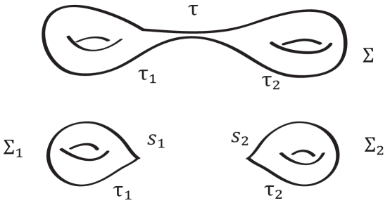
Figure 4. The separating degeneration of $\Sigma$ corresponds to $\tau\to 0$.

For the Heterotic strings, the right chirality blocks are governed by ordinary moduli space ${\mathcal{M}}_{2}$, which we shall parametrize by the period matrix $\tilde{\Omega}_{R}$,

(19.3) $$\tilde{\Omega}_{R}=\left(\begin{matrix}\tilde{\tau}_{1}&\tilde{\tau}\cr\tilde{\tau}&\tilde{\tau}_{2}\end{matrix}\right)$$

The right chiral amplitude, even after summation over spin structures, exhibit a singularity of the form $d\tilde{\tau}/\tilde{\tau}^{2}$ at the separating node; it is due to the presence of the identity operator (namely the zero-momentum tachyon). The presence of this singularity renders the integral over moduli space conditionally convergent, so that a precise prescription must be supplied in order to define it uniquely.

The full contribution to the vacuum energy is obtained by pairing the left and right chiral amplitudes and integrating the product over a cycle $\Gamma\subset\mathfrak{M}_{2}\times{\mathcal{M}}_{2}$. Along the cycle $\Gamma$, the relation between left super moduli and right moduli is complex conjugation, up to nilpotent terms,

(19.4) $$\bar{\Omega}_{R}^{*}=\hat{\Omega}+{\mathcal{O}}(\zeta^{1}\zeta^{2})$$

Near the separating degeneration node, the cycle $\Gamma$ may be parametrized by genus one moduli $\tau_{I}$ in terms of which we have,

$$\hat{\tau}_{I} = \tau_{I}$$

(19.5) $$\tilde{\tau}_{I} = \bar{\tau}_{I}$$

For the remaining even modulus $\tau$, we introduce a variable $t$ which parametrizes the degeneration, with $\tau=i\pi t/2$, as well as $\hat{\tau}=i\pi\hat{t}/2$ and $\tilde{\tau}=-i\pi\tilde{t}/2$. The odd-odd spin structure $\delta$ has vanishing contribution because ${\mathcal{Z}}[\delta]$ vanishes at the separating node. For the remaining 9 spin structures, ${\mathcal{Z}}[\delta]$ behaves as follows,

(19.6) $${\mathcal{Z}}[\delta]={1\over\hat{t}^{3/2}}\prod_{I=1,2}{\langle\nu_{0}|\delta_{I}\rangle\,\vartheta[\delta_{I}](0,\tau_{I})^{4}\over S_{\delta_{I}}(q_{I}-s_{I};\tau_{I})\,\vartheta^{\prime}_{1}(0,\tau_{I})^{4}}+{\mathcal{O}}\left({1\over\hat{t}^{1/2}}\right)$$

On each genus one component $\Sigma_{I}$ of the degeneration, with $I=1,2$, we denote the restricted even spin structure by $\delta_{I}$, the Szego kernel by $S_{\delta_{I}}(q_{I}-s_{I};\tau_{I})$, the point of support of $\chi$ by $q_{I}$, and the puncture by $s_{I}$, as illustrated in Figure 4. Finally, $\nu_{0}$ denotes the unique genus one odd spin structure on either $\Sigma_{I}$.

The relation between the components $\tau$ and $\hat{\tau}$, respectively of the period and super period matrix, near the separating degeneration node, reads as follows,

(19.7) $$\hat{t}=t-t^{1\over 2}{\zeta^{1}\zeta^{2}\over 2\pi^{2}}\prod_{I=1,2}S_{\delta_{I}}(q_{I}-s_{I};\tau_{I})$$

Away from the separating node the identification should satisfy $\tilde{t}^{*}=\hat{t}$, while near the node we should have instead $\tilde{t}^{*}=t$. Following [W3], we may parametrize $\Gamma$ with the help of a smooth interpolating function $h(t,\bar{t})$, which has the property that $h(t,\bar{t})=0$ for $|t|>1$ and $h(0,0)=1$, so that $\tilde{t}=\bar{t}$ along with,

(19.8) $$\qquad\hat{t}^{1\over 2}=t^{1\over 2}-h(t,\bar{t})\,{\zeta^{1}\zeta^{2}\over 4\pi^{2}}\prod_{I=1,2}S_{\delta_{I}}(q_{I}-s_{I};\tau_{I})$$

To examine the measure of integration over $\Gamma$, we introduce the regular coordinate $\rho=t^{1\over 2}$, so that the leading singular part of the measure near $\rho=0$ becomes,

(19.9) $$d\zeta^{1}d\zeta^{2}\,{d\hat{\rho}\over\hat{\rho}^{2}}\,{d\tilde{t}\over\tilde{t}^{2}}$$

An argument of homogeneity and scaling given in [W3] may be used to extract the contributions from the integration over $\Gamma$ near $t=0$. It requires scale invariance in $\tilde{t}$, along with scale invariance under $\hat{\rho}\to\lambda^{2}\hat{\rho}$ and $d\zeta\to\lambda^{-1}d\zeta$. To disentangle these contributions, we turn to the decomposition of orbits of spin structures and twists under the modular subgroup which leaves the separating node invariant.

20. Orbits under the modular subgroup $SL(2,{\mathbb{Z}})_{1}\times SL(2,{\mathbb{Z}})_{2}$

The separating degeneration node is left invariant under the modular subgroup $SL(2,{\mathbb{Z}})_{1}\times SL(2,{\mathbb{Z}})_{2}$ of the full $Sp(4,{\mathbb{Z}})$. Irreducible orbits of twists and spin structures under $Sp(4,{\mathbb{Z}})$ decompose into smaller irreducible orbits under this subgroup. The orbit of 10 even spin structures $\delta$ decomposes into one irreducible orbit of 9 even-even spin structures, and one odd-odd – which does not contribute.

The twists in the orbits ${\mathcal{O}}_{\gamma}$ under $Sp(4,{\mathbb{Z}})$, with $\gamma=0,1,2,3$ produce vanishing contributions upon summation over spin structure and the use of genus one Riemann identities. Contributions from ${\mathcal{O}}_{-}$ also vanish as the associated spin structures can never all be even, as pointed out already in section 17.

Thus, we are left with twists in orbit ${\mathcal{O}}_{+}$ only, and they decompose under $SL(2,{\mathbb{Z}})_{1}\times SL(2,{\mathbb{Z}})_{2}$ into two irreducible orbits, which we denote by ${\mathcal{O}}_{+}^{e}$ and ${\mathcal{O}}_{+}^{o}$. These orbits may be distinguished as follows. For $\mathfrak{e}\in{\mathcal{O}}_{+}^{e}$, the four spin structures in the set ${\mathcal{D}}[\mathfrak{e}]$ all descend to even-even under separating degeneration, while for $\mathfrak{e}\in{\mathcal{O}}_{+}^{o}$, one of the four spin structures in ${\mathcal{D}}[\mathfrak{e}]$ descends to odd-odd.

The separating degeneration properties due to the twisted fermion fields differ in the orbits ${\mathcal{O}}_{+}^{e}$ and ${\mathcal{O}}_{+}^{o}$. To see this, we note that their partition function, for both left and right chiralities, is proportional to (17.1) times its chiral conjugate,

(20.1) $$\prod_{\delta\in{\mathcal{D}}[\mathfrak{e}]}\vartheta[\delta](0,\hat{\Omega})\,\vartheta[\delta](0,\tilde{\Omega})$$

Note that, in addition to the contributions from the 6 twisted fermion fields, we are also including here the contribution of two untwisted fermions, in order to express the product simply over all the elements of ${\mathcal{D}}[\mathfrak{e}]$. We shall return to this issue later when we count the contributions form the untwisted right chirality fermions in section 21.

For $\mathfrak{e}\in{\mathcal{O}}_{+}^{e}$, the leading behavior is $\hat{t}^{0}\tilde{t}^{0}$ as $t\to 0$. But for $\mathfrak{e}\in{\mathcal{O}}_{+}^{o}$, it is $\hat{t}\tilde{t}$ due to the presence of one odd-odd spin structure amongst the four $\delta$ in the product. Moreover, the parity of higher order terms follows this pattern as well, and we have,

$$\mathfrak{e}\in{\mathcal{O}}_{+}^{e} d\zeta^{1}d\zeta^{2}\,{d\hat{\rho}\over\hat{\rho}^{2}}\,{d\tilde{t}\over\tilde{t}^{2}}\Big{(}1+\hat{c}_{e}\hat{t}^{2}+\tilde{c}_{e}\tilde{t}^{2}+\cdots\Big{)}$$

(20.2) $$\mathfrak{e}\in{\mathcal{O}}_{+}^{o} d\zeta^{1}d\zeta^{2}\,d\hat{\rho}\,{d\tilde{t}\over\tilde{t}}\Big{(}1+\hat{c}_{o}\hat{t}^{2}+\tilde{c}_{o}\tilde{t}^{2}+\cdots\Big{)}$$

where $\hat{c}_{e},\tilde{c}_{e},\hat{c}_{o}$ and $\tilde{c}_{o}$ are constants.

Carrying out the integration over $d\zeta^{1}d\zeta^{2}$, the dependence on $S_{\delta_{I}}(q_{I}-s_{I},\tau_{I})$ in the partition function ${\mathcal{Z}}[\delta]$ in (19.6) is cancelled by the same factor multiplying $\zeta^{1}\zeta^{2}$ in (19.8), so that the contribution from the boundary of $\mathfrak{M}_{2}$ to the vacuum energy is independent of the gauge choices $q_{I}$. In the formulation of [W3], slice independence is built in from the outset.

21. Heterotic $E_{8}\times E_{8}$ versus $Spin(32)/{\mathbb{Z}}_{2}$

The remaining factors, due to the contribution from the twisted bosons and the 26 untwisted fermions of right chirality, and the GSO sign factors $C_{\delta}[\mathfrak{e}]$ in (16.1) and (16.6) may be grouped together into the following factor,

(21.1) $${\mathcal{S}}=(\overline{\Psi_{4}})^{1-n}\sum_{\mathfrak{e}\in{\mathcal{O}}_{+}^{o}}\sum_{\delta\in{\mathcal{D}}[\mathfrak{e}]}\sum_{\delta_{R}\in{\mathcal{D}}[\mathfrak{e}]}C_{\delta}[\mathfrak{e}]C_{\delta_{R}}[\mathfrak{e}]\langle\delta_{0}|\delta\rangle\,(\overline{\vartheta[\delta_{R}]})^{4+8n}$$

The Heterotic strings are distinguished by the value assigned to $n$. For $E_{8}\times E_{8}$ we have $n=0$, and the 16 untwisted right chirality fermions of the unbroken $E_{8}$ give rise to the modular form $\Psi_{4}$, while the 10 fermions of the $E_{6}$ combine to give the factor $(\overline{\vartheta[\delta_{R}]})^{4}$. For $Spin(32)/{\mathbb{Z}}_{2}$, we have $n=1$, and all remaining 26 untwisted right chirality fermions combine to give the factor $(\overline{\vartheta[\delta_{R}]})^{12}$. In both cases, the contribution from two right chirality untwisted fermions was already taken into account in the factor (20.1), and must be omitted here to avoid double counting.

To perform the sums over spin structures in (21.1), we use the fact that modular invariance dictates a simple relation between the spin structures within the set ${\mathcal{D}}[\mathfrak{e}]$, which may be expressed as follows,

$$C_{\delta}[\mathfrak{e}] = C_{\delta_{*}}[\mathfrak{e}]\,\langle\delta_{*}|\delta\rangle$$

(21.2) $$C_{\delta_{R}}[\mathfrak{e}] = C_{\delta_{*}}[\mathfrak{e}]\,\langle\delta_{*}|\delta_{R}\rangle$$

for an arbitrary reference spin structure $\delta_{*}\in{\mathcal{D}}[\mathfrak{e}]$. Using the fact that for the spin structures $\delta,\delta_{*},\delta_{R},\delta_{0}\in{\mathcal{D}}[\mathfrak{e}]$ for $\mathfrak{e}\in{\mathcal{O}}_{+}^{o}$, we have,

$$\langle\delta_{*}|\delta\rangle\,\langle\delta|\delta_{R}\rangle\,\langle\delta_{R}|\delta_{*}\rangle = +1$$

(21.3) $$\langle\delta_{0}|\delta\rangle\,\langle\delta|\delta_{R}\rangle\,\langle\delta_{R}|\delta_{0}\rangle = +1$$

as well as the fact that $C_{\delta_{*}}[\mathfrak{e}]\,^{2}=1$, we find that the summand is independent of $\delta$, so that the sum over $\delta\in{\mathcal{D}}[\mathfrak{e}]$ gives a factor of 4, and we have,

(21.4) $${\mathcal{S}}=4(\overline{\Psi_{4}})^{1-n}\sum_{\mathfrak{e}\in{\mathcal{O}}_{+}^{o}}\sum_{\delta_{R}\in{\mathcal{D}}[\mathfrak{e}]}\langle\delta_{0}|\delta_{R}\rangle\,(\overline{\vartheta[\delta_{R}]})^{4+8n}$$

The sums may now be carried out explicitly, in the limit of separating degeneration, as is suitable for the boundary contributions of the separating node. The final results, obtained in [DP13], are consistent with the predictions made in [W3].

$E_{8}\times E_{8}$ Heterotic string, $n=0$

The sum over $\delta_{R}$ vanishes by the genus one Riemann identity, so that ${\mathcal{S}}=0$. As a result, the two-loop vacuum energy arising from the boundary of $\mathfrak{M}_{2}$ cancel, and the total vacuum energy is zero. This is consistent with the pattern of gauge symmetry breaking for this case, and the lack of a commuting $U(1)$ gauge group factor.

$Spin(32)/{\mathbb{Z}}_{2}$ Heterotic string, $n=1$

The sum over $\delta_{R}$ and $\mathfrak{e}$ is given by,

$${\mathcal{S}}=9216\times\bar{\eta}(\tau_{1})^{12}\times\bar{\eta}(\tau_{2})^{12}$$

and does not vanish. The remaining integrals over $\tau_{I}$ become proportional to the volume integrals for the corresponding genus one moduli spaces, and may be readily performed. As a result, the two-loop vacuum energy for the $Spin(32)/{\mathbb{Z}}_{2}$ theory arising from the boundary of $\mathfrak{M}_{2}$ is non-zero, and the total vacuum energy is non-zero. This result as well is consistent with the pattern of gauge symmetry breaking, and the appearance of a commuting $U(1)$ gauge group factor.

References

- [ABK] I. Antoniadis, C. Bachas, and C. Kounnas, “Four-dimensional superstrings”, Nucl. Phys. B289 (1987) 87
- [ADP] K. Aoki, E. D’Hoker and D.H. Phong, “Two loop superstrings on orbifold compactifications,” Nucl. Phys. B 688, 3 (2004) [hep-th/0312181].
- [ADS] J.J. Atick, L.J. Dixon and A. Sen, “String Calculation of Fayet-Iliopoulos d Terms in Arbitrary Supersymmetric Compactifications,” Nucl. Phys. B 292, 109 (1987).
- [AS] J.J. Atick and A. Sen, “Two Loop Dilaton Tadpole Induced By Fayet-iliopoulos D Terms In Compactified Heterotic String Theories,” Nucl. Phys. B 296, 157 (1988).
- [BM] N. Berkovits and C.R. Mafra, “Equivalence of two-loop superstring amplitudes in the pure spinor and RNS formalisms,” Phys. Rev. Lett. 96, 011602 (2006) [hep-th/0509234].
- [BE] Z. Bern, S. Davies, T. Dennen and Y. -t. Huang, “Absence of Three-Loop Four-Point Divergences in N=4 Supergravity,” Phys. Rev. Lett. 108, 201301 (2012) [arXiv:1202.3423 [hep-th]].
- [B] D. Bernard, “Z(2) Twisted Fields And Bosonization On Riemann Surfaces,” Nucl. Phys. B 302, 251 (1988).
- [C1] S.L. Cacciatori, F. Dalla Piazza and B. van Geemen, “Modular Forms and Three Loop Superstring Amplitudes,” Nucl. Phys. B 800, 565 (2008) [arXiv:0801.2543 [hep-th]].
- [C2] S.L. Cacciatori, F.D. Piazza and B. van Geemen, “Genus four superstring measures,” Lett. Math. Phys. 85, 185 (2008) [arXiv:0804.0457 [hep-th]].
- [C3] P. Candelas, G.T. Horowitz, A. Strominger and E. Witten, “Vacuum Configurations for Superstrings,” Nucl. Phys. B 258, 46 (1985).
- [C] A. Capelli, E. Castellani, F. Colomo, and P. Di Vecchia, eds. The Birth of String Theory, Cambridge University Press, 2012.
- [D] P. Deligne, P. Etingof, D.S. Freed, L.C. Jeffrey, D. Kazhdan, J.W. Morgan, D.R. Morrison, and E. Witten, editors, Quantum Fields and Strings: A course for Mathematicians, Vols 1, 2, American Mathematical Society, Institute for Advanced Study, 1999.
- [DG] E. D’Hoker and M. B. Green, “Zhang-Kawazumi Invariants and Superstring Amplitudes,” arXiv:1308.4597 [hep-th].
- [DGPR] E. D’Hoker, M.B. Green, B. Pioline, and R. Russo, to appear.
- [DGP] E. D’Hoker, M. Gutperle and D.H. Phong, “Two-loop superstrings and S-duality,” Nucl. Phys. B 722, 81 (2005) [hep-th/0503180].
- [DP1] E. D’Hoker and D.H. Phong, “The Geometry of String Perturbation Theory,” Rev. Mod. Phys. 60, 917 (1988), and references therein
- [DP2] E. D’Hoker and D.H. Phong, Superstrings, Super Riemann Surfaces, and Supermoduli Space, in Symposia Mathematica, String Theory, Vol XXXIII (Academic Press London and New York, 1990).
- [DP3] E. D’Hoker and D.H. Phong, “Conformal Scalar Fields And Chiral Splitting On Superriemann Surfaces,” Commun. Math. Phys. 125, 469 (1989).
- [DP4] E. D’Hoker and D.H. Phong, “The Box graph in superstring theory,” Nucl. Phys. B 440, 24 (1995) [hep-th/9410152].
- [DP5] E. D’Hoker, D.H. Phong, “Two loop superstrings. I. Main formulas,” Phys. Lett. B 529, 241 (2002) [hep-th/0110247].
- [DP6] E. D’Hoker, D.H. Phong, “Two loop superstrings. II. The chiral measure on moduli space,” Nucl. Phys. B 636, 3 (2002) [hep-th/0110283].
- [DP7] E. D’Hoker and D.H. Phong, “Two loop superstrings IV: The Cosmological constant and modular forms,” Nucl. Phys. B 639, 129 (2002) [hep-th/0111040].
- [DP8] E. D’Hoker and D.H. Phong, “Lectures on two loop superstrings,” Conf. Proc. C 0208124, 85 (2002) [hep-th/0211111].
- [DP9] E. D’Hoker and D.H. Phong, “Two-loop superstrings. V. Gauge slice independence of the N-point function,” Nucl. Phys. B 715, 91 (2005) [hep-th/0501196].
- [DP10] E. D’Hoker and D.H. Phong, “Two-loop superstrings VI: Non-renormalization theorems and the 4-point function,” Nucl. Phys. B 715, 3 (2005) [hep-th/0501197].
- [DP11] E. D’Hoker and D.H. Phong, “Two-Loop Superstrings. VII. Cohomology of Chiral Amplitudes,” Nucl. Phys. B 804, 421 (2008) [arXiv:0711.4314 [hep-th]].
- [DP12] E. D’Hoker and D.H. Phong, “Asyzygies, modular forms, and the superstring measure II,” Nucl. Phys. B 710, 83 (2005) [hep-th/0411182].
- [DP13] E. D’Hoker and D.H. Phong, “Two-loop vacuum energy for Calabi-Yau orbifold models,” Nucl. Phys. B 877, 343 (2013) [arXiv:1307.1749].
- [DVV] R. Dijkgraaf, E. Verlinde, and H. Verlinde, “ conformal field theories on Riemann surfaces”, Commun. Math. Phys. 115 (1988) 649-690.
- [DIS] M. Dine, I. Ichinose and N. Seiberg, “F Terms and D Terms in String Theory,” Nucl. Phys. B 293, 253 (1987).
- [DSW] M. Dine, N. Seiberg and E. Witten, “Fayet-Iliopoulos Terms in String Theory,” Nucl. Phys. B 289, 589 (1987).
- [DHVW] L.J. Dixon, J.A. Harvey, C. Vafa and E. Witten, “Strings on Orbifolds. 2.,” Nucl. Phys. B 274, 285 (1986).
- [DF] R. Donagi and A.E. Faraggi, “On the number of chiral generations in Z(2) x Z(2) orbifolds,” Nucl. Phys. B 694, 187 (2004) [hep-th/0403272].
- [DW] R. Donagi and E. Witten, “Supermoduli Space Is Not Projected,” arXiv:1304.7798 [hep-th].
- [F] J. Fay, Theta Functions on Riemann surfaces, Springer Lecture Notes in Mathematics, Vol 352, Springer-Verlag, Berlin, 1973.
- [FI] P. Fayet and J. Iliopoulos, “Spontaneously Broken Supergauge Symmetries and Goldstone Spinors,” Phys. Lett. B 51, 461 (1974).
- [FMS] D. Friedan, E.J. Martinec and S.H. Shenker, “Conformal Invariance, Supersymmetry and String Theory,” Nucl. Phys. B 271, 93 (1986).
- [GM] H. Gomez and C.R. Mafra, “The closed-string 3-loop amplitude and S-duality,” arXiv:1308.6567 [hep-th].
- [GS] M.B. Green and J.H. Schwarz, “Supersymmetrical String Theories,” Phys. Lett. B 109, 444 (1982).
- [GS1] M.B. Green and S. Sethi, “Supersymmetry constraints on type IIB supergravity,” Phys. Rev. D 59, 046006 (1999) [arXiv:hep-th/9808061].
- [GV] M.B. Green and P. Vanhove, “The low energy expansion of the one-loop type II superstring amplitude,” Phys. Rev. D 61, 104011 (2000) [arXiv:hep-th/9910056].
- [GRV] M.B. Green, J.G. Russo and P. Vanhove, “Modular properties of two-loop maximal supergravity and connections with string theory,” JHEP 0807, 126 (2008) [arXiv:0807.0389 [hep-th]].
- [GHMR] D.J. Gross, J.A. Harvey, E.J. Martinec and R. Rohm, “The Heterotic String,” Phys. Rev. Lett. 54, 502 (1985).
- [G] S. Grushevsky, “Superstring scattering amplitudes in higher genus,” Commun. Math. Phys. 287, 749 (2009) [arXiv:0803.3469 [hep-th]].
- [GM1] S. Grushevsky and R.S. Manni, “The superstring cosmological constant and the Schottky form in genus 5,” Am. J. Math. 133, 1007 (2011) [arXiv:0809.1391 [math.AG]].
- [I] J.I. Igusa, Theta Functions, Springer-Verlag, Berlin, 1972.
- [M1] E.J. Martinec, “Nonrenormalization Theorems and Fermionic String Finiteness,” Phys. Lett. B 171, 189 (1986).
- [MV1] M. Matone and R. Volpato, “Superstring measure and non-renormalization of the three-point amplitude,” Nucl. Phys. B 806, 735 (2009) [arXiv:0806.4370 [hep-th]].
- [MV2] M. Matone and R. Volpato, “Getting superstring amplitudes by degenerating Riemann surfaces,” Nucl. Phys. B 839, 21 (2010) [arXiv:1003.3452 [hep-th]].
- [MV3] M. Matone and R. Volpato, “Higher genus superstring amplitudes from the geometry of moduli space,” Nucl. Phys. B 732, 321 (2006) [hep-th/0506231].
- [M2] A. Morozov, “NSR Superstring Measures Revisited,” JHEP 0805, 086 (2008) [arXiv:0804.3167 [hep-th]].
- [NSW] K.S. Narain, M.H. Sarmadi and E. Witten, “A Note on Toroidal Compactification of Heterotic String Theory,” Nucl. Phys. B 279, 369 (1987).
- [OP] N.A. Obers and B. Pioline, “U duality and M theory,” Phys. Rept. 318, 113 (1999) [hep-th/9809039].
- [RSV] A.A. Rosly, A.S. Schwarz, and A.A. Voronov, “Geometry of Superconformal Manifolds”, Commun. Math. Phys. 119 (1988) 129-152.
- [SM] R. Salvati-Manni, “Remarks on Superstring amplitudes in higher genus,” Nucl. Phys. B 801, 163 (2008) [arXiv:0804.0512 [hep-th]].
- [T] P. Tourkine and P. Vanhove, “An non-renormalisation theorem in N=4 supergravity,” Class. Quant. Grav. 29, 115006 (2012) [arXiv:1202.3692 [hep-th]].
- [W1] E. Witten, “Notes On Super Riemann Surfaces And Their Moduli,” arXiv:1209.2459 [hep-th].
- [W2] E. Witten, “Superstring Perturbation Theory Revisited,” arXiv:1209.5461 [hep-th].
- [W3] E. Witten, “More On Superstring Perturbation Theory,” arXiv:1304.2832 [hep-th].
- [W4] E. Witten, “Notes On Holomorphic String And Superstring Theory Measures Of Low Genus,” arXiv:1306.3621 [hep-th].
- [W5] E. Witten, “The Feynman in String Theory,” arXiv:1307.5124 [hep-th].