Critical Casimir interactions around the consolute point of a binary solvent

Abstract

Spatial confinement of a near-critical medium changes its fluctuation spectrum and modifies the corresponding order parameter distribution. These effects result in effective, so-called critical Casimir forces (CCFs) acting on the confining surfaces. These forces are attractive for like boundary conditions of the order parameter at the opposing surfaces of the confinement. For colloidal particles dissolved in a binary liquid mixture acting as a solvent close to its critical point of demixing, one thus expects the emergence of phase segregation into equilibrium colloidal liquid and gas phases. We analyze how such phenomena occur asymmetrically in the whole thermodynamic neighborhood of the consolute point of the binary solvent. By applying field-theoretical methods within mean-field approximation and the semi-empirical de Gennes-Fisher functional, we study the CCFs acting between planar parallel walls as well as between two spherical colloids and their dependence on temperature and on the composition of the near-critical binary mixture. We find that for compositions slightly poor in the molecules preferentially adsorbed at the surfaces, the CCFs are significantly stronger than at the critical composition, thus leading to pronounced colloidal segregation. The segregation phase diagram of the colloid solution following from the calculated effective pair potential between the colloids agrees surprisingly well with experiments and simulations.

I Introduction

Finite-size contributions to the free energy of a spatially confined fluid give rise to an excess pressure, viz., an effective force per unit area acting on the confining surfaces. This so-called solvation force depends on the geometry of the confinement, the surface separation, the fluid-fluid interactions, the substrate potentials exhibited by the surfaces, and on the thermodynamic state of the fluid Evans (1990). The solvation force acquires a universal, long-ranged contribution upon approaching the bulk critical point of the fluid, as first pointed out by Fisher and de Gennes Fisher and de Gennes (1978). This is due to critical order parameter fluctuations which led to the notion of ‘critical Casimir forces’, in analogy with the quantum-mechanical Casimir forces which are due to quantum fluctuations of confined electromagnetic fields Casimir (1948).

The important role of critical Casimir forces (CCFs) for colloidal suspensions has implicitly been first recognized while studying experimentally aggregation phenomena in binary near-critical solvents Beysens and Estève (1985). Numerous other experimental studies followed aiming to clarify important aspects of the observed phenomenon, such as its reversibility and the location of its occurrence in the temperature - composition phase diagram of the solvent (see, for example, Refs. Beysens and Narayanan (1999); *Gallagher-et:1992b; *Narayanan-et:1993; *Kurnaz-et:1997; Bonn et al. (2009); *Gambassi-et:2010Ibid; *Bonn-et:2010Ibid; Veen et al. (2012) and references therein). Measurements were performed mostly in the homogeneous phase of the liquid mixture. They demonstrate that the temperature - composition $(T,c)$ region within which colloidal aggregation occurs is not symmetric about the critical composition $c_{c}$ of the solvent mixture. Strong aggregation occurs on that side of the critical composition which is rich in the component disfavored by the colloids. More recently, reversible fluid-fluid and fluid-solid phase transitions of colloids dissolved in the homogeneous phase of a binary liquid mixture have been observed Guo et al. (2008); Nguyen et al. (2013); Dang et al. (2013). These experiments also show that the occurrence of such phase transitions is related to the affinity of the colloidal surfaces for one of the two solvent components as described above.

Various mechanisms for attraction between the colloids, which can lead to these phenomena, have been suggested. The role of dispersion interactions, which are effectively modified in the presence of an adsorption layer around the colloidal particles, has been discussed in Ref. Law et al. (1998). A “bridging” transition, which occurs when the wetting films surrounding each colloid merge to form a liquid bridge Archer et al. (2005), provides a likely mechanism sufficiently off the critical composition of the solvent. However, in the close vicinity of the bulk critical point of the solvent, in line with the prediction by Fisher and de Gennes Fisher and de Gennes (1978), attraction induced by critical fluctuations should dominate.

In the original argument by Fisher and de Gennes, the scaling analysis for off-critical composition of the solvent has not been carried out. Due to the lack of explicit results for the composition dependence of CCFs, for a long time it has not been possible to quantitatively relate the aggregation curves to CCFs. Rather, it was expected that CCFs play a negligible role for off-critical compositions because away from $c_{c}$ the bulk correlation length, which determines the range of CCFs, shrinks rapidly. However, to a certain extent the properties of an aggregation region can be captured by assuming the attraction mechanism to be entirely due to CCFs. This has been shown in a recent theoretical study which employs an effective one-component description of the colloidal suspensions Mohry et al. (2012a); *Mohry-et:2012bIbid. Such an approach is based on the assumption of additivity of CCFs and requires the knowledge of the critical Casimir pair potential in the whole neighborhood of the critical point of the binary solvent, i.e., as a function of both temperature and solvent composition close to $(T_{c},c_{c})$. In Ref. Mohry et al. (2012a); *Mohry-et:2012bIbid, it was assumed that colloids are spheres all strongly preferring the same component of the binary mixture such that they impose symmetry breaking ($(+,+)$) boundary conditions Diehl (1997) on the order parameter of the solvent. Further, the pair potential between two spheres has been expressed in terms of the scaling function of the CCFs between two parallel plates by using the Derjaguin approximation Derjaguin (1934). The dependence of the CCFs on the solvent composition translates into the dependence on the bulk ordering field $h_{b}$ conjugate to the order parameter (see Eq. (A4) in the first part of Ref. Mohry et al. (2012a)). For the parallel-plate (or film) geometry in spatial dimension $D{}=3$, the latter has been approximated by the functional form obtained within mean-field theory (MFT, $D{}=4$) by using the field-theoretical approach within the framework of Landau-Ginzburg theory. The scaling functions of the CCFs resulting from these approximations have not yet been reported in the literature. We present them here for a wide range of parameters. In order to assess the quality of the approximations adopted in Ref. Mohry et al. (2012a, b) we calculate the scaling functions of the CCFs by using alternative theoretical approaches and compare the corresponding results.

In this spirit, one can estimate how well the mean-field functional form, which is exact in $D{}=4$ (up to logarithmic corrections), approximates the dependence on $h_{b}$ of CCFs for films in $D{}=3$ by comparing it with the form obtained from the local-functional approach Fisher and Upton (1990a); *Fisher-et:1990bIbid in $D{}=3$. We use the semi-empirical free energy functional developed by Fisher and Upton Fisher and Upton (1990a); *Fisher-et:1990bIbid in order to extend the original de Gennes-Fisher critical-point ansatz Fisher and de Gennes (1978). Upon construction, this functional fulfills the necessary analytic properties as function of $T$ and a proper scaling behavior for arbitrary $D$. The extended de Gennes-Fisher functional provides results for CCFs in films with $(+,+)$ boundary conditions at $h_{b}=0$, which are in a good agreement with results from Monte Carlo simulations Borjan and Upton (2008). A similar local-functional approach proposed by Okamoto and Onuki Okamoto and Onuki (2012) uses a renormalized Helmholtz free energy instead of the Helmholtz free energy of the linear parametric model used in Ref. Borjan and Upton (2008). Such a version does not seem to produce better results for the Casimir amplitudes Okamoto and Onuki (2012). This ‘renormalized’ local-functional theory has been recently applied to study the bridging transition between two spherical particles Okamoto and Onuki (2013). Some results for the CCFs with strongly adsorbing walls and $h_{b}\neq 0$ obtained within mean-field theory and within density functional theory in $D{}=3$ have been presented in Refs. Schlesener et al. (2003) and Buzzaccaro et al. (2010); *Piazza-et:2011, respectively. These results are consistent with the present ones.

We also explore the validity of the Derjaguin approximation for the mean-field scaling functions of the CCFs, focusing on their dependence on the bulk ordering field. For that purpose, we have performed bona fide mean-field calculations for spherical particles, the results of which can be viewed as exact for hypercylinders in $D=4$ or approximate for two spherical particles in $D=3$.

This detailed knowledge of the CCFs as function of $T$ and $h_{b}$ is applied in order to analyze recently published experimental data for the pair potential and the segregation phase diagram Dang et al. (2013) of poly-n-isopropyl-acrylamide microgel (PNIPAM) colloidal particles immersed in a near-critical 3-methyl-pyridine (3MP)/heavy water mixture.

Our paper is organized such that in Sec. II we discuss the theoretical background. In Sec. III.1, results for CCFs for films are presented. These results as obtained from the field-theoretical approach within mean-field approximation are compared with those stemming from the local functional approach. We discuss how the dependence of the CCFs on the bulk ordering field $h_{b}$ changes with the spatial dimension $D$. Section III.2 is devoted to the CCF between spherical particles, where we also probe the reliability of the Derjaguin approximation. In Sec. IV our theoretical results are confronted with the corresponding experimental findings and simulations. We provide a summary in Sec. V.

II Theoretical background

For the demixing phase transition of a binary liquid mixture, the order parameter $\phi$ is proportional to the deviation of the concentration $c={\varrho}_{A}-{\varrho}_{B}$ from its value $c_{c}$ at the critical point, i.e., $\phi\sim c-c_{c}$; here ${\varrho}_{\alpha}$, $\alpha\in\left\{A,B\right\}$, are the number densities of the particles of species $A$ and $B$, respectively. The bulk ordering field, conjugate to this order parameter, is proportional to the deviation of the difference $\Delta\mu=\mu_{A}-\mu_{B}$ of the chemical potentials $\mu_{\alpha}$, $\alpha\in\left\{A,B\right\}$, of the two species from its critical value, i.e., $h_{b}\sim\Delta\mu-\Delta\mu_{c}$. We note, that the actual scaling fields for real fluids are linear combinations of $h_{b}$ and the reduced temperature $t=\left(T_{c}-T\right)/T_{c}$ [$t=\left(T-T_{c}\right)/T_{c}$] for a lower [upper] critical point.

Close to the bulk critical point, the bulk correlation length attains the scaling form

$$\xi\left(t,h_{b}\right)=\xi_{t}I^{(D)}_{\pm}\left(\left|\mathsf{\Sigma}\right|=\xi_{t}/\xi_{h}\right),$$ (1)

where the universal bulk scaling function $I^{(D)}_{\pm}$ satisfies $I^{(D)}_{\pm}\left(\left|\mathsf{\Sigma}\right|\to 0\right)=1$ and $I^{(D)}_{\pm}\left(\left|\mathsf{\Sigma}\right|\to\infty\right)=\left|\mathsf{\Sigma}\right|^{-1}$. The functional form of $I^{(D)}_{\pm}\left(\left|\mathsf{\Sigma}\right|\right)$ depends on the sign $\left(\pm\right)$ of $t$, but not on the sign of the bulk scaling variable $\mathsf{\Sigma}$. It is suitable to define the latter as ${\mathrm{sgn}}\left(\mathsf{\Sigma}\right)={\mathrm{sgn}}\left(th_{b}\right)$. The bulk correlation length for $h_{b}=0$ is

$$\xi_{t}=\xi_{\pm}^{\left(0\right)}\left|t\right|^{-\nu}$$ (2a)

and

$$\xi_{h}=\xi_{h}^{\left(0\right)}\left|h_{b}\right|^{-\nu/\left(\beta\delta\right)}$$ (2b)

is the bulk correlation length along the critical isotherm. Here $\nu$, $\beta$, and $\delta=\left(D\nu/\beta\right)-1$ are standard bulk critical exponents. For the Ising bulk universality class considered here, $\nu=0.63$ and $\beta=0.33$ in spatial dimension $D=3$ and $\nu=\beta=1/2$ in $D\geq 4$  Fisher (1967); Pelissetto and Vicari (2002). There are three non-universal amplitudes, $\xi_{\pm}^{\left(0\right)}$ and $\xi_{h}^{\left(0\right)}$, but the ratio $U_{\xi}=\xi_{+}^{\left(0\right)}/\xi_{-}^{\left(0\right)}$ forms a universal number Pelissetto and Vicari (2002); Not (a), $U_{\xi}\left(D=3\right)\simeq 1.9$ and $U_{\xi}\left(D=4\right)=\sqrt{2}$. The values of $\xi_{\pm}^{\left(0\right)}$ and $\xi_{h}^{\left(0\right)}$ depend on the definition of $\xi$ which we take to be the true bulk correlation length governing the exponential decay of the two-point correlation function of the bulk order parameter.

II.1 Film geometry

For two parallel planar walls a distance $L$ apart the critical Casimir force is defined as Brankov et al. (2000); Gambassi (2009)

$$f_{C}^{\left(\parallel\right)}=-\frac{\partial\mathcal{F}_{sgl}^{\left(ex\right)}}{\partial L}=-\frac{\partial\left(\mathcal{F}_{sgl}-V\mathfrak{f}_{b,sgl}\right)}{\partial L},$$ (3)

where $\mathfrak{f}_{b,sgl}$ is the singular part of the bulk free energy density, $\mathcal{F}_{sgl}^{\left(ex\right)}$ is the singular part of the excess over the bulk free energy of the film, and $V=\mathcal{A}{}L$ where $\mathcal{A}$ is the macroscopically large surface area of one wall.

Finite-size scaling Barber (1983) predicts that Fisher and de Gennes (1978)

$$\frac{f_{C}^{\left(\parallel\right)}}{\mathcal{A}}=\frac{k_{B}T}{L^{D}}\tilde{\vartheta}_{\parallel}^{(D)}(\mathcal{Y}={\mathrm{sgn}}\left(t\right)L/\xi_{t},\Lambda={\mathrm{sgn}}\left(h_{b}\right)L/\xi_{h}),$$ (4)

where $k_{B}$ is the Boltzmann constant and $\tilde{\vartheta}_{||}^{(D)}(\mathcal{Y},\Lambda)$ is a universal scaling function. Its functional form depends on the bulk universality class and on the surface universality classes of the confining walls. Here we focus on walls with the same adsorption preferences (expressed in terms of surface fields conjugate to the order parameter at the surfaces) in the so-called strong adsorption limit in which $\phi\left(\mathbf{r}\right)\to\infty$ for the spatial coordinate $\mathbf{r}$ approaching the walls. Note that $\tilde{\vartheta}^{(D)}$ depends on the sign of $h_{b}$ because the surface fields at the confining walls break the bulk symmetry $h_{b}\to-h_{b}$. Depending on the particular thermodynamic path under consideration, other representations of the scaling function of the critical Casimir force might be more convenient. For example, the scaling function $\hat{\vartheta}_{||}^{(D)}\left(\mathcal{Y}={\mathrm{sgn}}\left(t\right)L/\xi_{t},\mathsf{\Sigma}={\mathrm{sgn}}(th_{b})\xi_{t}/\xi_{h}\right)$ lends itself to describe the dependence of the CCFs on $h_{b}$ at fixed temperature. We will discuss the following representations

$$\begin{split}&\tilde{\vartheta}_{\parallel}^{(D)}(\mathcal{Y},\Lambda)=\hat{\vartheta}_{\parallel}^{(D)}(\mathcal{Y},\mathsf{\Sigma}=\frac{\Lambda}{\mathcal{Y}}={\mathrm{sgn}}(th_{b})\frac{\xi_{t}}{\xi_{h}})=\\ &\bar{\vartheta}_{\parallel}^{(D)}(\Lambda,\mathsf{\Sigma})=\vartheta_{\parallel}^{(D)}(\mathsf{Y}=\frac{\mathcal{Y}}{I^{(D)}_{\pm}\left(\left|\mathsf{\Sigma}\right|\right)}={\mathrm{sgn}}(t)\frac{L}{\xi},\mathsf{\Sigma}).\end{split}$$ (5)

II.2 Colloidal particles

We consider two spherical colloids, or more generally two hypercylinders, in spatial dimension $D$. A hypercylinder $H_{D,d}$ has $d$ finite semiaxes of equal length $R$ and is translationally invariant in the remaining $\left(D-d\right)$ dimensions. Here, the two hypercylinders are assumed to be geometrically identical and aligned parallel to each other. We denote this geometry by $\circ\circ$. For two hypercylinders at closest surface-to-surface distance $L$, the CCF $f_{C}^{\left(\circ\circ\right)}$ is defined by the right hand side of Eq. (3) with $\mathcal{F}_{sgl}$ as the singular contribution to the free energy of the binary solvent in the macroscopically large volume $V$ with two suspended colloids.

The scaling function of the critical Casimir force between two hypercylinders $H_{D,d}$, per “length” $\mathit{l}$ of the $\left(D-d\right)$-dimensional hyperaxis, can be written as Schlesener et al. (2003); Kondrat et al. (2009)

$$\frac{f_{C}^{\left(\circ\circ\right)}}{\mathit{l}}=\frac{k_{B}T}{LL^{D-d}}\frac{1}{\Delta^{\left(d-1\right)/2}}\vartheta^{\left(D,d\right)}_{\circ\circ}\left(\mathcal{Y}={\mathrm{sgn}}\left(t\right)\frac{L}{\xi_{t}},\Delta=\frac{L}{R},\Lambda={\mathrm{sgn}}\left(h_{b}\right)\frac{L}{\xi_{h}}\right).$$ (6)

Within the Derjaguin approximation Derjaguin (1934) the total force between two spherical objects, $H_{3,3}$ or $H_{4,3}$, is taken to be ${f_{C}^{\left(\circ\circ\right)}}/{\mathit{l}}\simeq\int\mathrm{d}S\;\tilde{f}_{C}^{\left(\parallel\right)}=2\pi\int_{0}^{R}\mathrm{d}\rho\;\rho\tilde{f}_{C}^{\left(\parallel\right)}\left(L\left(\rho\right)\right)$, where $\tilde{f}_{C}^{\left(\parallel\right)}$ is the force per area and $L\left(\rho\right)=L+2R\left(1-\sqrt{1-\left(\rho/R\right)^{2}}\right)$, leading to the scaling function [compare with Eqs. (4) and (6)]

$$\vartheta^{\left(D,d\right)}_{\circ\circ,Derj}\left(\mathcal{Y},\Delta,\Lambda\right)=\pi\int\limits_{1}^{1+2\Delta^{-1}}\mathrm{d}x\;x^{-D}\left[1-\frac{\Delta}{2}\left(x-1\right)\right]\tilde{\vartheta}_{\parallel}^{(D)}\left(x\mathcal{Y},x\Lambda\right),\;\;(D,d)=(3,3)\mbox{ and }(4,3).$$ (7)

Note, that for $(D,d)=(4,4)$ in the expression for $\vartheta^{(4,4)}_{\circ\circ,Derj}$ there is an additional factor of $2\sqrt{(x-1)(1+\Delta(x-1)/4)}$ multiplying the integrand in Eq. (7). Commonly Hanke et al. (1998); Schlesener et al. (2003); Kondrat et al. (2009); Tröndle et al. (2009); *Troendle-et:2010; *LabbeLaurent-et:2014; Hasenbusch (2013), in this context [i.e., Eq. (7)] $\Delta$ is set to zero. Thus, within the Derjaguin approximation, $f_{C}^{\left(\circ\circ\right)}\sim\Delta^{-\left(d-1\right)/2}$ [Eq. (6)]. We adopt this approximation except for, c.f., Fig. 3(b), where we shall discuss the full dependence on $\Delta$ given by Eq. (7).

II.3 Landau theory

In the spirit of an expansion in terms of $\epsilon=4-D$, for the lowest order contribution we use the mean-field Landau-Ginzburg-Wilson theory in order to study the universal CCF in the film geometry (Sec. III.1) and between two colloidal particles (Sec. III.2). The Landau-Ginzburg-Wilson Hamiltonian, in units of $k_{B}T$, is given by  Binder (1983); Diehl (1986, 1997)

$$\mathcal{H}\left[\phi\left(\mathbf{r}\right)\right]=\int_{V}\left\{\frac{1}{2}\left(\nabla\phi\right)^{2}+\frac{\tau}{2}\phi^{2}+\frac{u}{4!}\phi^{4}-h_{b}\phi\right\}\textrm{\;d}^{D}r,$$ (8)

where $V$ is the volume of the confined critical medium, $\tau\propto t$ changes sign at the (mean-field) critical temperature $T_{c}$, and the quartic term with the coupling constant $u>0$ stabilizes the Hamiltonian in the ordered phase, i.e., for $\tau<0$. Equation (8) must be supplemented by appropriate boundary conditions, which for the critical adsorption fixed point correspond to $\phi\to\pm\infty$.

Within mean-field theory, the bulk correlation lengths [Eq. (2)] are Schlesener et al. (2003)

$$\xi_{t}\left(t>0\right)=\tau^{-1/2},\quad\xi_{t}\left(t<0\right)=\left|2\tau\right|^{-1/2},$$ (9a)

$$\xi_{h}\left(h_{b}\gtrless 0\right) =\left|\sqrt{{9u}/{2}}h_{b}\right|^{-1/3},$$ (9b)

and

$$\xi(t,h_{b})=\left\{\left[\xi_{t}\left(\left|t\right|\right)\right]^{-2}{\mathrm{sgn}}\left(t\right)+(u/2)\phi_{b}^{2}\left(t,h_{b}\right)\right\}^{-1/2},$$ (10)

where the bulk order parameter $\phi_{b}\left(t,h_{b}\right)$ satisfies $\left\{3\left[\xi_{t}\left(\left|t\right|\right)\right]^{-2}{\mathrm{sgn}}\left(t\right)+\frac{u}{2}\phi_{b}^{2}\right\}\sqrt{\frac{u}{2}}\phi_{b}=\left(\xi_{h}\right)^{-3}{\mathrm{sgn}}\left(h_{b}\right)$ so that $\frac{u}{2}\phi_{b}^{2}$ can be expressed in terms of $\xi_{t}$ and $\xi_{h}$ and inserted into Eq. (10). Within the present mean-field theory $\tau=\left[\xi_{+}^{\left(0\right)}\right]^{-2}t$.

The minimum of Eq. (8) gives the mean-field profile $\phi_{mf}\left(\mathbf{r};t,h_{b}\right)$. With this the critical Casimir force is

$$\boldsymbol{f_{C}}={k_{B}T}\int_{\mathcal{A}}\mathcal{T}(\phi)\cdot\boldsymbol{n}\;d^{D-1}r=\mathit{l}{k_{B}T}\int_{\mathcal{A}^{\prime}}\mathcal{T}(\phi)\cdot\boldsymbol{n}\;d^{d-1}r$$ (11)

where $\mathcal{A}$ is an arbitrary $\left(D-1\right)$-dimensional surface enclosing a colloid or separating two planes, $\mathcal{A}{}^{\prime}$ is its $\left(d-1\right)$-dimensional subset in the subspace in which the colloids have a finite extent, $\boldsymbol{n}$ is its unit outward normal, and

$$\mathcal{T}_{jk}\left(\phi\right)=\frac{\delta\mathtt{h}}{\delta\left(\partial_{k}\phi\right)}\left(\partial_{j}\phi\right)-\delta_{jk}\mathtt{h}$$ (12)

is the stress tensor Kondrat et al. (2009); here $\mathtt{h}\left(\phi\right)$ is the integrand in Eq. (8), and $\partial_{k}\phi=\partial\phi/\partial x_{k}$. For the film geometry with chemically and geometrically uniform surfaces, the integration in Eq. (11) amounts to the evaluation of $\mathcal{T}$ at an arbitrary point between the two surfaces. For two spherical particles, the surface of integration is an arbitrary surface that encloses one of the particles. Accordingly, the force between the particles is $\boldsymbol{f_{C}}=f_{C}\boldsymbol{e}$, where $\boldsymbol{e}$ is a unit vector along the line connecting their centers. We have minimized the Hamiltonian $\mathcal{H}$ numerically using the finite element method Kondrat and Tröndle .

Within mean-field theory, the scaling functions of the critical Casimir force can be determined only up to the prefactor $\sim 1/u$ (note that $u$ is dimensionless in $D=4$). In order to circumvent this uncertainty and to facilitate the comparison with experimental or other theoretical results, we shall normalize our mean-field results by the critical Casimir amplitude for the film geometry [see Eq. (4)] $\Delta^{\left(4\right)}_{\parallel}=\;\tilde{\vartheta}_{||}^{(D=4)}\left(\mathcal{Y}=0,\Lambda=0\right)=-\left(6/u\right){4}\left[K\left(1/2\right)\right]^{4}<0$ Krech (1997), where $K$ is the complete elliptic integral of the first kind. For the sphere-sphere geometry, one has Schlesener et al. (2003); Kondrat et al. (2009) $\vartheta^{\left(D=4,d=3\right)}_{\circ\circ}\left(\mathcal{Y}=0,\Delta=0,\Lambda=0\right)=\vartheta^{\left(D=4,d=3\right)}_{\circ\circ,Derj}\left(\mathcal{Y}=0,\Delta=0,\Lambda=0\right)=\frac{\pi}{3}\tilde{\vartheta}_{\parallel}^{(D=4)}\left(\mathcal{Y}=0,\Lambda=0\right)=\frac{\pi}{3}\vartheta_{\parallel}^{(D=4)}\left(\mathsf{Y}=0,\mathsf{\Sigma}\right)$; note that $\mathsf{\Sigma}={\mathrm{sgn}}(th_{b})\xi_{t}/\xi_{h}=const$ defines implicitly various thermodynamic paths $h_{b}(t)$ which, however, all pass the critical point $(t=0,h_{b}=0)$, i.e., $\mathsf{Y}=0$ [see Fig. 1]. Accordingly, $\vartheta^{(D)}(\mathsf{Y}=0,\mathsf{\Sigma})$ does not depend on $\mathsf{\Sigma}$. Thus normalization by $\tilde{\vartheta}_{||}^{(D=4)}\left(0,0\right)$ eliminates the prefactor $\frac{1}{u}$. This holds also for nonzero values of $\mathcal{Y}$, $\Delta$, and $\Lambda$ as well as beyond the Derjaguin approximation.

II.4 Extended de Gennes-Fisher functional

For the film geometry, we consider the ansatz for the free energy functional proposed by Fisher and Upton Fisher and Upton (1990a, b)

$$\mathrm{F}\left[\Phi\left(z\right)\right]=\mathcal{A}{}\int_{-L/2}^{L/2}\left[\frac{\xi^{2}(\Phi,t)}{2\chi(\Phi,t)}(\partial\Phi)^{2}+W\left(\Phi,t,h_{b}\right)\right]\textrm{\;d}{z}+\mathrm{F}_{s},$$ (13)

where $\partial\Phi=\partial{\Phi}/\partial{z}$. The equilibrium profile $\Phi_{eq}$ is taken as the one which minimizes $\mathrm{F}$. $\mathrm{F}\left[\Phi_{eq}\right]$ is the singular part of the free energy of the near-critical medium confined in the film. Note that the order parameter $\Phi$ in Eq. (13) is dimensionless, unlike $\phi$ in the Landau model, in which it has the dimension $\left(\text{length}\right)^{1-D/2}$ [see Eq. (8)]. The surface contribution $\mathrm{F}_{s}=-h_{s,1}\phi\left(z=-L/2\right)-h_{s,2}\phi\left(z=L/2\right)$ implements the boundary conditions. We consider walls adsorbing the same species corresponding to surface fields $h_{s,1}=h_{s,2}>0$. $W\left(\Phi;t,h_{b}\right)$ is the excess (over the bulk) free energy density (in units of $k_{B}T$), $\xi\left(\Phi;t\right)$ and $\chi\left(\Phi;t\right)$ are the bulk correlation length and the susceptibility of a homogeneous bulk system at $\left(\Phi,t\right)$, respectively Fisher and Upton (1990b).

Minimizing the functional given by Eq. (13) leads to an Euler-Lagrange equation, which can be formally integrated. One then proceed by taking the scaling limit of this latter first integral and by using the scaling forms of the following bulk quantities:

$$W\left(\Phi;t,h_{b}\right)=\left|\Phi\right|^{\delta+1}Y_{\pm}\left(\Psi,\mathsf{\Sigma}\right)\\$$ (14a)

and

$$\xi^{2}/\left(2\chi\right)=\left|\Phi\right|^{\eta\nu/\beta}Z_{\pm}\left(\Psi\right),$$ (14b)

where $\Psi=\Phi/\Phi_{b}\left(-\left|t\right|,h_{b}=0\right)=\left|t\right|^{-\beta}\Phi/\mathcal{B}_{t}$. The (dimensionless) non-universal amplitude $\mathcal{B}_{t}$ of the bulk order parameter $\Phi_{b}$ can be expressed via universal amplitude ratios in terms of the non-universal amplitudes $\xi_{+}^{\left(0\right)}$ and $\xi_{h}^{\left(0\right)}$ of the bulk correlation length Pelissetto and Vicari (2002); the functions $\tilde{Y}_{\pm}\left(\Psi,\Sigma\right)=Y_{\pm}\left(\Psi,\Sigma\right)/Y_{+}\left(\infty,0\right)$ and $\tilde{Z}_{\pm}\left(\Psi\right)=Z_{\pm}\left(\Psi\right)/Z_{+}\left(\infty\right)$ are universal. This procedure determines (even without knowing the explicit functional forms of $\tilde{Y}_{\pm}$ and $\tilde{Z}_{\pm}$) a formal expression for the scaling function $\hat{\vartheta}_{||}^{(D)}$ of the CCF Borjan (1999); Borjan and Upton (2008). Here we take into account the additional dependence on the scaling variable $\mathsf{\Sigma}{}\neq 0$ and obtain for $\mathcal{Y}>0$ Mohry (2013)

$$\hat{\vartheta}_{||}^{(D)}\left(\mathcal{Y}>0,\mathsf{\Sigma}\right)=-A_{1}\left|\mathcal{Y}\right|^{2-\alpha}{\Psi_{m}}^{\left(1+\delta\right)}\tilde{Y}_{+}\left(\Psi_{m},\mathsf{\Sigma}\right),$$ (15)

where $A_{1}=R_{\chi}Q_{c}/\left(\delta+1\right)$ is a universal number which is expressed in terms of the universal amplitude ratios Pelissetto and Vicari (2002); Not (a) $R_{\chi}$, $Q_{2}$, and $Q_{c}$. $\Psi_{m}$ is defined through $\Phi_{m}=\Phi(z=z_{m})=\Psi_{m}\Phi_{b}(-\left|t\right|,h_{b}=0)$, which for the present case $h_{s,1},h_{s,2}>0$ is the minimal value of the order parameter profile across the film.

In order to calculate the critical Casimir force from Eq. (15) one has to evaluate the functions $Y_{\pm}$ and $Z_{\pm}$ in Eq. (14). The analytical expressions of these functions can be obtained by using the so-called linear parametric representation Schofield (1969); *Josephson:1969; *Fisher:1971; Pelissetto and Vicari (2002); Borjan and Upton (2008). For given $\mathcal{Y}$ and $\mathsf{\Sigma}$ the scaling function of the critical Casimir force is then computed numerically (for details see Ref. Mohry (2013)).

III Numerical results

III.1 Critical Casimir forces in films

Our mean-field results for the behavior of the Casimir scaling function around the consolute point of the binary solvent are summarized in Fig. 1 in terms of the scaling function $\vartheta^{\left(D=4\right)}_{\parallel}\left(\mathsf{Y}={\mathrm{sgn}}\left(t\right)L/\xi\left(t,h_{b}\right),\mathsf{\Sigma}={\mathrm{sgn}}\left(th_{b}\right)\xi_{t}/\xi_{h}\right)$. This particular scaling form turns out to be particularly suitable in view of the Derjaguin approximation used below for the sphere-sphere geometry because the dependence of the CCF on $L$, measured in units of the true bulk correlation length $\xi\left(t,h_{b}\right)$, enters $\vartheta^{\left(D=4\right)}_{\parallel}$ only via $\mathsf{Y}$. The second scaling variable $\mathsf{\Sigma}$, which depends on the thermodynamic state of the solvent, varies smoothly from $\mathsf{\Sigma}=0$ at the bulk coexistence curve to $\mathsf{\Sigma}=\pm\infty$ at the critical isotherm.

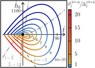
Figure 1: Behavior of the normalized mean-field Casimir scaling function $\vartheta^{\left(D=4\right)}_{\parallel}\left(\mathsf{Y}={\mathrm{sgn}}\left(t\right)L/\xi\left(t,h_{b}\right),\mathsf{\Sigma}={\mathrm{sgn}}\left(th_{b}\right)\xi_{t}/\xi_{h}\right)$ along lines of constant scaling variable $\left|\mathsf{Y}\right|=4,5,\ldots,10$ (from the inner to the outermost ring) in the thermodynamic state space of the solvent spanned by $\hat{t}=\left(L/\xi_{+}^{\left(0\right)}\right)^{1/\nu}t$ and $\hat{h}_{b}=\left(L/\xi_{h}^{\left(0\right)}\right)^{\beta\delta/\nu}h_{b}$. The color along the lines of constant $\left|\mathsf{Y}\right|$ indicates the absolute value $|\vartheta^{\left(D=4\right)}_{\parallel}|$. The bulk critical point of the solvent $(\hat{t},\hat{h}_{b})=(0,0)$ is indicated by $\bullet$. The region shown here lies above the capillary transition critical point $\left(\mathsf{Y}_{\parallel,c}=-11,\mathsf{\Sigma}_{\parallel,c}=1.3\right)$ Schlesener et al. (2003), where the film coexistence line ends. For $(+,+)$ boundary conditions, the capillary condensation transition occurs for $\hat{t}<0$ and $\hat{h}_{b}<0$. The dash-dotted lines indicate the thermodynamic paths $\mathsf{\Sigma}=1$ and $=3$ and the dashed line the path of constant order parameter $\hat{}\phi=\frac{L}{\xi_{+}^{\left(0\right)}}\phi/\mathcal{B}_{t}=-5$. Within mean-field theory $\nu=1/2$ and $\nu/\left(\beta\delta\right)=1/3$. $\Delta_{\parallel}^{\left(D=4\right)}=|{\vartheta}^{\left(D=4\right)}_{\parallel}\left(\mathsf{Y}=0,\mathsf{\Sigma}\right)|$, which is independent of $\mathsf{\Sigma}$.

In Fig. 1, we have plotted several lines of constant scaling variable $\left|\mathsf{Y}\right|=L/\xi\left(t,h_{b}\right)=4,5,\ldots,10$ in the thermodynamic space of the solvent spanned by $\hat{t}=\left(L/\xi_{+}^{\left(0\right)}\right)^{1/\nu}t$ and $\hat{h}_{b}=\left(L/\xi_{h}^{\left(0\right)}\right)^{\beta\delta/\nu}h_{b}$. The shape of the lines $\left|\mathsf{Y}\right|=\mathrm{const}$ is determined by the bulk correlation length $\xi(t,h_{b})$. Therefore it is symmetric about the $\hat{t}$-axis. A break of slope occurs at the bulk coexistence line $\left(\hat{t}<0,\hat{h}_{b}=0\right)$ because $\xi\left(t,h_{b}\right)$ depends on the bulk order parameter $\phi_{b}$ [see Eq. (10)] which varies there discontinously. We use the color code to indicate the strength $|\vartheta^{\left(D=4\right)}_{\parallel}|$ of the Casimir scaling function along these lines. For $\left(+,+\right)$ boundary conditions the critical Casimir force in a slab is attractive and accordingly $\vartheta^{\left(D=4\right)}_{\parallel}<0$ for all values of $t$ and $h_{b}$.

The main message conveyed by Fig. 1 is the asymmetry of the critical Casimir force around the critical point of the solvent with the maximum strength occurring at $h_{b}<0$. This asymmetry is due to the presence of surface fields which break the bulk symmetry $h_{b}\to-h_{b}$ of the system and shift the phase coexistence line away from the bulk location $h_{b}=0$. In the film with $(+,+)$ boundary conditions the shifted, so-called capillary condensation transition, occurs for negative values of $h_{b}$ Evans (1990); Nakanishi and Fisher (1983). At capillary condensation, the solvation force (which within this context is a more appropriate notion than the notion of the critical Casimir force) exhibits a jump from a large value for thermodynamic states corresponding to the $\left(+\right)$ phase to a vanishingly small value for those corresponding to the $\left(-\right)$ phase. Above the two-dimensional plane spanned by $(\hat{t},\hat{h}_{b})$, the surface $\vartheta^{\left(D=4\right)}_{\parallel}$ forms a trough which is the remnant of these jumps extending to the thermodynamic region above the capillary condensation critical point, even to temperatures higher than $T_{c}$. This trough, reflecting the large strengths visible in Fig. 1 for $\hat{h}_{b}<0$, deepens upon approaching the capillary condensation point.

Along the particular thermodynamic path of zero bulk field (i.e., $\mathsf{\Sigma}=0$) the minimum is located above $T_{c}$ and has the value $\vartheta^{\left(4\right)}_{\parallel}\left(\mathsf{Y}_{min}=3.8,\mathsf{\Sigma}=0\right)=1.4\times{}\vartheta^{\left(4\right)}_{\parallel}\left(0,0\right)$. Along the critical isotherm (i.e., $\left|\mathsf{\Sigma}\right|=\infty$) one has $\vartheta^{\left(4\right)}_{\parallel}\left(\mathsf{Y}_{min}=8.4,\mathsf{\Sigma}=-\infty\right)=10\times{}\vartheta^{\left(4\right)}_{\parallel}\left(0,0\right)$. Interestingly, along all lines $\left|\mathsf{Y}\right|=L/\xi\left(t,h_{b}\right)=\mathrm{const}$ the strength $|\vartheta^{\left(4\right)}_{\parallel}\left(\mathsf{Y}=\mathrm{const},\mathsf{\Sigma}\right)|$ takes its minimal value at the bulk coexistence curve $h_{b}=0^{+}$. For $\left|\mathsf{Y}\right|\gtrless 6.3$ the maximal value of $|\vartheta^{\left(4\right)}_{\parallel}\left(\mathsf{Y}=\mathrm{const},\mathsf{\Sigma}\right)|$ is located at $h_{b}<0$ and $t\lessgtr 0$.

It is useful to consider the variation of the scaling function of the CCF along the thermodynamic paths of fixed $\mathsf{\Sigma}$. As examples, such paths are shown for $\mathsf{\Sigma}=1$ and $\mathsf{\Sigma}=3$ in Fig. 1 as dash-dotted lines. Thermodynamic paths corresponding to $0<\mathsf{\Sigma}\lesssim 1.3$ cross the phase boundary of coexisting phases in the film at certain values $\mathsf{Y}_{cx}\left(\mathsf{\Sigma}\right)$, which lie outside the range of the plot in Fig. 1. Along the paths corresponding to $0<\mathsf{\Sigma}\lesssim 3$, $\vartheta^{\left(4\right)}_{\parallel}\left(\mathsf{Y},\mathsf{\Sigma}=const<3\right)$ as function of $\mathsf{Y}$ has two minima. The local minimum occurs above $T_{c}$, whereas the global one occurs below $T_{c}$. For all other fixed values of $\mathsf{\Sigma}$, the scaling function $\vartheta^{\left(4\right)}_{\parallel}$, as function of $\mathsf{Y}$, exhibits a single minimum; for negative $\mathsf{\Sigma}$ it is located above $T_{c}$ (i.e., $\mathsf{Y}{}>0$), whereas for $\mathsf{\Sigma}\gtrsim 3$ below $T_{c}$ (i.e., $\mathsf{Y}{}<0$). Results for $\vartheta^{\left(D=4\right)}_{\parallel}$ as function of $\mathsf{Y}={\mathrm{sgn}}\left(t\right)L/\xi\left(t,h_{b}\right)$ for constant values of $\mathsf{\Sigma}={\mathrm{sgn}}\left(th_{b}\right)\xi_{t}/\xi_{h}$ are shown in Ref. Mohry (2013).

Thermodynamic paths of constant order parameter $\phi\neq 0$ are particularly experimentally relevant, because they correspond to a fixed off-critical composition of the solvent. As an example Fig. 1 shows the case $\hat{\phi}=\frac{L}{\xi_{+}^{\left(0\right)}}\phi/\mathcal{B}_{t}=-5$ as indicated by the dashed line. Within mean-field theory this path varies linearly with $t$.

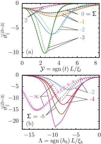
Figure 2: Two representations of the scaling function of the critical Casimir force for the film geometry with $(+,+)$ boundary conditions [Eq. (5)]: (a) $\hat{\vartheta}^{(D=3)}_{\parallel}\left(\mathcal{Y},\mathsf{\Sigma}\right)$ plotted versus $\mathcal{Y}={\mathrm{sgn}}\left(t\right)L/\xi_{t}$ and (b) $\bar{\vartheta}^{(D=3)}_{\parallel}\left(\Lambda,\mathsf{\Sigma}\right)$ plotted versus $\Lambda={\mathrm{sgn}}\left(h_{b}\right)L/\xi_{h}$ for several values of the scaling variable $\mathsf{\Sigma}{}={\mathrm{sgn}}\left(th_{b}\right)\xi_{t}/\xi_{h}$. The full lines are the results obtained from the local functional approach together with the linear parametric model [Eq. (15)], and the dashed lines correspond to the dimensional approximation [Eq. (16)]. In (b) the symbols are Monte Carlo data from Ref. Vasilyev and Dietrich (2013) for $\mathsf{\Sigma}=-\infty$. We note that thermodynamic states corresponding to $\mathsf{\Sigma}=-\infty$ and $\mathsf{\Sigma}=\infty$ are the same; they form the critical isotherm.

In Ref. Mohry et al. (2012a); *Mohry-et:2012bIbid, the mean-field results described above were used in order to approximate the dependence of the CCFs on the bulk ordering field $h_{b}$ in spatial dimension $D=3$:

$$\hat{\vartheta}^{(D)}_{\parallel}\left(\mathcal{Y},\mathsf{\Sigma}\right)\simeq\hat{\vartheta}^{(D)}_{\parallel}\left(\mathcal{Y},\mathsf{\Sigma}=0\right)\frac{\hat{\vartheta}^{(D^{\prime}=4)}_{\parallel}\left(\mathcal{Y},\mathsf{\Sigma}\right)}{\hat{\vartheta}^{(D^{\prime}=4)}_{\parallel}\left(\mathcal{Y},\mathsf{\Sigma}=0\right)},$$ (16)

where $\hat{\vartheta}^{(D=3)}_{\parallel}\left(\mathcal{Y},\mathsf{\Sigma}=0\right)$ is taken from Monte Carlo simulation data Vasilyev et al. (2009). This “dimensional approximation” is inspired by the observation that the trends and qualitative features of $\hat{\vartheta}^{(D)}_{\parallel}$ are the same for different values of $D$ Vasilyev et al. (2007); *Vasilyev-et:2009; Mohry et al. (2010). The characteristics of this approximation are as follows: (i) For $D\to D^{\prime}=4$, i.e., for mean-field theory, the right hand side of Eq. (16) turns into the correct expression for the full range of all scaling variables. (ii) For $h_{b}\to 0$ (i.e., $\mathsf{\Sigma}\to 0$) the right hand side of Eq. (16) reduces exactly to $\hat{\vartheta}^{(D)}_{\parallel}\left(\mathcal{Y},\mathsf{\Sigma}=0\right)$ for all values $D$, $D^{\prime}$, and $\mathcal{Y}$. In this sense the approximation is concentrated on the dependence on $h_{b}$. (iii) For $D^{\prime}=4$ the approximation can be understood as the lowest order contribution in an $\epsilon=4-D$ expansion of $\zeta_{\vartheta{}_{\parallel}}^{\left(D\right)}={\hat{\vartheta}^{(D)}_{\parallel}\left(\mathcal{Y},\mathsf{\Sigma}\right)}/{\hat{\vartheta}^{(D)}_{\parallel}\left(\mathcal{Y},\mathsf{\Sigma}=0\right)}$ which carries the whole dependence of the CCFs on $\mathsf{\Sigma}$. As a ratio, the mean-field expression for $\zeta_{\vartheta{}_{\parallel}}^{\left(D^{\prime}=4\right)}$ does not suffer from the amplitude of $\hat{\vartheta}^{(D^{\prime}=4)}_{\parallel}$ being undetermined. In Eq. (16), the scaling variables $\mathcal{Y}$ and $\mathsf{\Sigma}$ are taken to involve the critical bulk exponents in spatial dimension $D$ so that the approximation concerns only the shape of the scaling function. The use of bulk critical exponents in spatial dimension $D$ for scaling variables which, however, are arguments of the scaling function in spatial dimension $D^{\prime}\neq D$, may lead to a deviation from the proper asymptotic behavior. However, this potential violation of the proper asymptotic behavior of the scaling function of the CCFs is expected to occur for large values of the arguments of the scaling function for which its value is exponentially small. Thus, the potential violation should not matter quantitatively in the range of the values of $\mathcal{Y}$ and $\mathsf{\Sigma}$ for which the scaling function $\hat{\vartheta}^{(D)}_{\parallel}$ attains noticeable values. Here we compare this approximation with the results obtained from the extended de Gennes-Fisher functional using the linear parametric model.

In Fig. 2(a) we plot $\hat{\vartheta}_{||}^{(D=3)}(\mathcal{Y},\mathsf{\Sigma})$ as a function of $\mathcal{Y}>0$ for several values of $\mathsf{\Sigma}$. For large values of $\left|\mathsf{\Sigma}\right|$ the relevant part of the corresponding thermodynamic path is close to the critical isotherm and accordingly the scaling variable $\Lambda=\mathsf{\Sigma}\mathcal{Y}={\mathrm{sgn}}\left(h_{b}\right)L/\xi_{h}$ is more appropriate than the scaling variable $\mathcal{Y}$. Therefore, in Fig. 2(b) we show $\bar{\vartheta}_{||}^{(D=3)}(\Lambda,\mathsf{\Sigma})=\hat{\vartheta}_{||}^{(D=3)}(\Lambda/\mathsf{\Sigma},\mathsf{\Sigma})$ as a function of $\Lambda$ for several fixed values of $\mathsf{\Sigma}\leq-2$.

As can be inferred from Fig. 2 the dimensional approximation in Eq. (16) works well for weak bulk fields (such that $\left|\mathsf{\Sigma}\right|<3$). Although the minima of the scaling functions are slightly shifted relative to each other, the depths of these minima compare well with the results of the local functional approach. For all $\left|\mathsf{\Sigma}\right|<\infty$, the value $\mathcal{Y}=0$ corresponds to the bulk critical point and thus at $\mathcal{Y}=0$ the curves $\hat{\vartheta}^{(D)}_{\parallel}$ attain the same value [see Fig. 2(a)].

For strong bulk fields, i.e., $\mathsf{\Sigma}<-4$ the dimensional approximation [Eq. (16)] fails [see Fig. 2(b)]. For example, $|\bar{\vartheta}^{(D=3)}_{\parallel}|$ of the approximative curve becomes smaller for more negative values of $\mathsf{\Sigma}$, which is in contrast to the results of mean-field theory and of the local functional approach. This wrong trend of the results of the dimensional approximation is explained in detail in Ref. Mohry (2013).

We note that the scaling functions $\vartheta^{\left(D=3\right)}_{\parallel}$ of the critical Casimir force as obtained from the local functional exhibit the same qualitative features as the ones calculated within mean-field theory. For example, the position $\mathsf{Y}_{min}\left(\mathsf{\Sigma}\right)$ of the minimum as obtained from the present local functional theory changes from $\mathsf{Y}_{min}\left(\mathsf{\Sigma}=0\right)=\mathcal{Y}_{min}\left(\mathsf{\Sigma}=0\right)=3.1$ at the thermodynamic path $h_{b}=0$ towards $\mathsf{Y}_{min}\left(\mathsf{\Sigma}=-\infty\right)=-\Lambda_{min}\left(\mathsf{\Sigma}=-\infty\right)=9.4$ at the critical isotherm. These values are similar to the ones obtained from mean-field theory. The results of the local functional approach are peculiar with respect to the cusp-like minimum for curves close to the critical isotherm [for $\left|\mathsf{\Sigma}\right|=\infty$, i.e., $t=0$, see Fig. 2(b)]. Such a behavior is also reported for the similar approach used in Ref. Okamoto and Onuki (2012). However, there is no such cusp in the Monte Carlo data for $t=0$, i.e., $\left|\mathsf{\Sigma}\right|=\infty$, Vasilyev and Dietrich (2013) [see the symbols in Fig. 2(b)]. As compared with the results of the local functional, the minimum of $\bar{\vartheta}^{\left(D=3\right)}_{\parallel}(\Lambda,\left|\mathsf{\Sigma}\right|=\infty)$ obtained from Monte Carlo simulations is less deep and is positioned at a more negative value of $\Lambda$. For $\Lambda>0$ [not shown in Fig. 2(b)], $\bar{\vartheta}^{\left(D=3\right)}_{\parallel}(\Lambda,\left|\mathsf{\Sigma}\right|=\infty)$ as obtained from the local functional is less negative than the corresponding scaling function obtained from the Monte Carlo simulations.

We observe that upon decreasing the spatial dimension $D$ the ratio of the strengths $\left|\hat{\vartheta}^{(D)}_{\parallel}\right|$ at its two extrema, the one located at the critical isotherm and the other located at $h_{b}=0$, increases, from $7$ in $D=4$ to $11.5$ (local functional) or $8$ (Monte Carlo simulations) in $D=3$, and to $15$ in $D=2$ Drzewiński et al. (2000).

III.2 Critical Casimir forces between spherical colloids

The CCF between two spherical colloids takes the form given by Eq. (6); here we take $d=3$ and $D=4$. In order to calculate $\vartheta^{\left(4,3\right)}_{\circ\circ}$, we use the stress tensor $\mathcal{T}(\phi)$ [see Eqs. (11) and Eq. (12)] with the mean-field profile $\phi(\mathbf{r})$ which is determined by minimizing the Hamiltonian in Eq. (8) numerically using GSL gsl and F3DM Kondrat and Tröndle defined on three-dimensional meshes generated by TETGEN  Si .

CCFs between spherical colloids in zero bulk field have been widely studied in the literature Hanke et al. (1998); Schlesener et al. (2003); Burkhardt and Eisenriegler (1995); Hasenbusch (2013). Whereas so far the mean-field theory of the Landau model has only been considered for four-dimensional spheres $H_{D=4,d=4}$, here we focus on three-dimensional spheres, i.e., on hypercylinders $H_{3,3}$ or $H_{D\geq 4,3}$. We first consider the corresponding CCFs in zero bulk field $\left(\Lambda=0\right)$. We recall that we consider $(+,+)$ boundary conditions only.

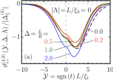
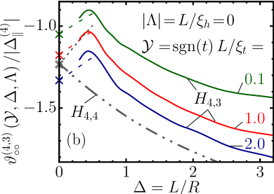
Figure 3: The critical Casimir force between two like colloids in zero bulk field ($\Lambda=0$) as obtained from the mean-field theory of the Landau model. (a) The normalized scaling function $\vartheta^{\left(D=4,d=3\right)}_{\circ\circ}$ versus $\mathcal{Y}={\mathrm{sgn}}\left(t\right)L/\xi_{t}$ for five values of $\Delta=L/R$, where $L$ is the surface-to-surface distance between two spheres $H_{4,3}$ of radius $R$. The curve $\Delta=0$ corresponds to the Derjaguin approximation. (b) The normalized scaling function $\vartheta^{\left(4,3\right)}_{\circ\circ}$ versus $\Delta$ for three values of $\mathcal{Y}>0$. The results of the Derjaguin approximation as given by Eq. (7) are shown as dashed lines ($\Delta\to 0$) and by crosses ($\Delta=0$). We recall the relation $\vartheta^{\left(D=4,d=3\right)}_{\circ\circ}\left(\mathcal{Y}=0,\Delta=0,\Lambda=0\right)=\frac{\pi}{3}\tilde{\vartheta}_{\parallel}^{(D=4)}\left(0,0\right)=\frac{\pi}{3}\Delta_{\parallel}^{(4)}$. For comparison, the scaling function $\vartheta^{\left(D=4,d=4\right)}_{\circ\circ}$ at the critical point ($\mathcal{Y}=\Lambda=0$) for spheres $H_{4,4}$ Schlesener et al. (2003) is shown by the grey dash-dotted line. The Derjaguin approximation for $H_{4,4}$ (corresponding to the grey dotted line emerging from the grey cross) displays, as a function of $\Delta$, a trend opposite to the result $\vartheta^{\left(D=4,d=4\right)}_{\circ\circ}$ obtained from the full calculation.

The scaling function $\vartheta^{\left(4,3\right)}_{\circ\circ}\left(\mathcal{Y},\Delta=\mathrm{const},\Lambda=0\right)$, as a function of $\mathcal{Y}$, has a shape which is typical for like boundary conditions [see Fig. 3(a)]. Interestingly, the magnitude of $\vartheta^{\left(4,3\right)}_{\circ\circ}$ depends non-monotonically on $\Delta$. This is shown explicitly in Fig. 3(b), where the scaling function is plotted versus $\Delta$ for three values of $\mathcal{Y}={\mathrm{sgn}}(t)L/\xi_{t}>0$. In Fig. 3(b), $\vartheta^{\left(4,3\right)}_{\circ\circ}$ approaches the scaling function of the Derjaguin approximation from above when $\Delta\to 0$, but decreases upon increasing $\Delta>\Delta_{m}$, where $\Delta_{m}\approx 1/2$ seems to be almost independent of $\mathcal{Y}$ (in the range of $\mathcal{Y}$ shown). This non-monotonic behavior is unlike the case of four-dimensional spheres in $D=4$ dimension (i.e., $H_{4,4}$ hypercylinders), for which the scaling function approaches its value at $\Delta=0$ from below and exhibits no maxima (grey dash-dotted line in Fig. 3(b) reproduced from Ref. Schlesener et al. (2003)). For the wall-sphere geometry, such a non-monotonic behavior of the scaling function of the CCF for $\Delta\to 0$ has been found for a sphere $H_{3,3}$ using Monte Carlo simulations Hasenbusch (2013), but not for (hyper)cylinders $H_{4,d}$, $d\in\left\{2,3\right\}$, treated by mean-field theory Tröndle et al. (2009); *Troendle-et:2010; *LabbeLaurent-et:2014.

The behavior of $\vartheta^{\left(4,3\right)}_{\circ\circ}$ for large $\Delta\gg 1$ is not quite clear due to technical difficulties associated with large mesh sizes and the increasing numerical inaccuracy; moreover, in this limit, the force attains very small values.

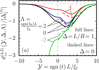
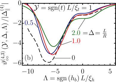
Figure 4: Effect of the bulk field $\left(\Lambda\neq 0\right)$ on the scaling function $\vartheta^{\left(D=4,d=3\right)}_{\circ\circ}$ of the critical Casimir force [Eq. (6)] as obtained from the mean-field theory for the Landau model. (a) Normalized $\vartheta^{\left(4,3\right)}_{\circ\circ}$ shown as a function of $\mathcal{Y}={\mathrm{sgn}}\left(t\right)L/\xi_{t}$ for $\Delta=L/R=1$ (full lines) and within the Derjaguin approximation ($\Delta=0$, dashed lines) for four values of $\Lambda={\mathrm{sgn}}\left(h_{b}\right)L/\xi_{h}$. (b) Normalized $\vartheta^{\left(4,3\right)}_{\circ\circ}$ shown as a function of $\Lambda$ for $\mathcal{Y}=1$ and for four values of $\Delta$. The curves are normalized with the critical Casimir amplitude $\Delta_{\parallel}^{\left(4\right)}$ for the film.

Results for nonzero bulk fields $h_{b}$ are shown in Fig. 4. For fixed sphere radii $R$ and fixed surface-to-surface distance $L$, the curves in Fig. 4(a) for fixed $\Lambda$ correspond to varying the temperature along the thermodynamic paths of iso-fields $h_{b}=\mathrm{const}$. For fixed $L$, the curves in Fig. 4(b) compare the scaling function of the CCF as function of $h_{b}$ along the supercritical isotherm $T_{c}<T=\mathrm{const}$ for various sphere sizes.

For $h_{b}>0$ the variation of $\vartheta^{\left(4,3\right)}_{\circ\circ}$ with $\mathcal{Y}$ resembles the features observed for vanishing $h_{b}$ in the case of the sphere-sphere or film geometry, i.e., $\vartheta^{\left(4,3\right)}_{\circ\circ}$ exhibits a minimum located above $T_{c}$ ($\mathcal{Y}>0$) [compare Fig. 4(a) with Figs. 3(a) and 2]. Upon increasing the bulk field, the magnitude of the scaling function decreases and the position of the minimum shifts towards larger $\mathcal{Y}$. This is in line with the behavior for the film geometry (Fig. 1).

The behavior of the scaling function for negative bulk fields is different. For positive $\mathcal{Y}$, there is still a residual minimum of the scaling function located very close to $\mathcal{Y}=0$, which disappears upon decreasing $h_{b}$. This is already the case for $\Lambda=-2$ in Fig. 4(a). This disappearance is in line with the results for film geometry. For negative $\mathcal{Y}$, at a certain value $\Lambda<0$, in films capillary condensation occurs whereas between spherical colloids a bridging transition takes place Archer et al. (2005); Okamoto and Onuki (2013); Bauer et al. (2000). Near these phase transitions, the effective force acting between the confining surfaces is attractive and becomes extremely strong; the depth of the corresponding effective interaction potentials can reach a few hundred $k_{B}T$. This concomitant enormous increase of the strength of the force is also reflected in the universal scaling function [see the green line $\Lambda=-2$ in Fig. 4(a) for $\mathcal{Y}<0$]. (For the film geometry this issue has been discussed in detail in Ref. Schlesener et al. (2003); in particular, Fig. 11 in Ref. Schlesener et al. (2003) exhibits a cusp in the scaling function in the vicinity of the capillary condensation; similarly, upon decreasing $\mathcal{Y}$, called $\Theta_{-}$ in Ref. Schlesener et al. (2003), to negative values the magnitude of the scaling function increases strongly.)

It is also interesting to note a non-monotonic dependence of the scaling function $\vartheta^{\left(4,3\right)}_{\circ\circ}$ on $\Delta=L/R$ [Fig. 4(b)]. For positive bulk fields, $\left|\vartheta^{\left(4,3\right)}_{\circ\circ}\right|$ is stronger for larger $\Delta$. This is different, however, for negative bulk fields, for which $\left|\vartheta^{\left(4,3\right)}_{\circ\circ}\right|$ is stronger for smaller $\Delta$. Such an increase of $\left|\vartheta^{\left(4,3\right)}_{\circ\circ}\right|$ upon decreasing $\Delta$ holds also for zero bulk field [see Fig. 3(b) for $\Delta\gtrsim 1/2$].

Finally, for larger values of $\Delta=L/R$ the deficiencies of the Derjaguin approximation are clearly visible in Figs. 3 and 4.

IV Comparison with experimental data

IV.1 Effective interaction potentials

In Ref. Dang et al. (2013), the pair distribution function $g\left(r\right)$ of poly-n-isopropyl-acrylamide microgel (PNIPAM) colloidal particles immersed in a near-critical 3-methyl-pyridine (3MP)/heavy water mixture has been determined experimentally for various deviations $\Delta T=T_{c}-T$ from the lower critical temperature $T_{c}\approx 39^{\circ}\textrm{C}$ (of the miscibility gap of the bulk 3MP/heavy water mixture without colloidal particles). Here we analyze the experimental data for the 3MP mass fraction $\omega=0.28$ which is close to the critical value (see below).

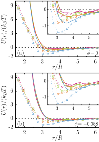
Figure 5: Effective interaction potential $U_{exp}$ as determined experimentally in Ref. Dang et al. (2013) (symbols, dashed lines as a guide to the eye) and its background contribution $U_{bck}$ (full lines). The experimental system consists of colloidal particles of radius $R\approx 250\;\mathrm{nm}$ immersed in a near critical binary liquid mixture. The effective potential was determined for various deviations $\Delta T=T_{c}-T$ from the lower critical point $T_{c}$, at $\Delta T/\textrm{K}=0.6$ ($\boldsymbol{\times}$, magenta), $0.5$ ($\boldsymbol{\Box{}}$, green), $0.4$ ($\boldsymbol{\circ}$, orange), and $0.3$ ($\boldsymbol{\bigtriangleup}$, blue). Upon approaching $T_{c}$ the minimum of the potential $U$ deepens due to the attractive Casimir interaction. The ‘background’ part of the potential is obtained by subtracting the critical Casimir potential $U_{c}$ [see Eqs. (17)and (18)]. If $U_{bck}$ was temperature independent the various full lines would collapse. In (a) the binary liquid mixture used in the experiments (mass fraction $\omega=0.28$) is assumed to be at its critical composition $\omega=\omega_{c}=0.28$, whereas (b) corresponds to a slightly off-critical composition $\widetilde{}\phi=\left(\omega_{c}-\omega\right)/\mathcal{B}_{t}=-0.088$. In (b) one observes a better collapse of the full lines than in (a). The critical Casimir potential $U_{c}$ depends on $\mathsf{\Sigma}$, which is directly related to $\widetilde{\phi{}}$ via the equation of state $\mathsf{\Sigma}=E\left(\left|t\right|^{\beta}\widetilde{\phi}\right)$ (see the main text). The curves correspond to the value $\xi_{+}^{\left(0\right)}=1.5\;\textrm{nm}$ [Eq. (2a)]. The colloidal particles are soft, so that $U_{exp}\left(r<2R\right)>0$ and very large but not infinite.

We assume that the solvent-mediated interaction between the PNIPAM colloids for center-to-center distances $r$ is the sum of a background contribution $U_{bck}$ and the critical Casimir potential $U_{c}$. This assumption is valid for small salt concentrations Pousaneh and Ciach (2011); *Bier-et:2011; *Pousaneh-et:2012 which is the case for the samples studied in Ref. Dang et al. (2013). Accordingly, one has

$$U_{bck}\left(r\right)=U_{exp}\left(r;\Delta T\right)-U_{c}\left(r;\Delta T\right).$$ (17)

Within the studied temperature range $\Delta T<1\mathrm{K}$ this ‘background’ contribution is expected to depend only weakly on temperature and hence we consider it to be temperature independent. We use the potential of mean-force in order to extract the experimentally determined interaction potential $U_{exp}\left(r\right)=-k_{B}T{}\ln\left[g\left(r\right)\right]$. This relation is reliable for small solute densities, as they have been used in the experiments. Therefore only small deviations are expected to occur by using more accurate expressions for the potential, such as the hypernetted chain or the Percus-Yevick closures.

Since the numerical calculation of the critical Casimir potential in the bona fide sphere-sphere geometry for all parameters which are needed for comparison with experiment is too demanding, here we resort to the Derjaguin approximation. Within this approximation the critical Casimir potential $U_{c}$ between two colloids of radius $R$ [Eqs. (6) and (7)] is Derjaguin (1934); Hanke et al. (1998); Tröndle et al. (2009); *Troendle-et:2010

$$U_{c}\left(r;\Delta T,\omega\right)=\pi k_{B}T\frac{R}{r-2R}\int_{1}^{\infty}\mathrm{d}x\left(x^{-2}-x^{-3}\right)\hat{\vartheta}^{\left(D=3\right)}_{\parallel}\left(x\mathcal{Y},\mathsf{\Sigma}\right),$$ (18)

where $\mathcal{Y}={\mathrm{sgn}}\left(t\right)\left(r-2R\right)/\xi_{t}$ and $\mathsf{\Sigma}={\mathrm{sgn}}\left(th_{b}\right)\xi_{t}/\xi_{h}$. The dependence of $U_{c}$ on temperature and on the mass fraction of the solvent is captured by the bulk correlation lengths $\xi_{t}$ and $\xi_{h}$ of the solvent, respectively [Eq. (2)]. In order to calculate the scaling function $\hat{\vartheta}^{\left(D=3\right)}_{\parallel}$ of the critical Casimir force between two planar walls we use the local functional approach (see Sec. II.4).

For the amplitude of the thermal bulk correlation length we take $\xi_{+}^{\left(0\right)}=1.5\;\mathrm{nm}$, which we extracted from the experimental data presented in Ref. Sorensen and Larsen (1985). However, in the literature there are no well established data for the critical mass fraction $\omega_{c}$ of the 3MP/heavy water binary liquid mixtures. In Ref. Cox (1952), the value $\omega_{c}=0.28$ is quoted while the scaling analysis of Fig. 1 in Ref. Cox (1952) suggests the value $\omega_{c}\approx 0.29$. The inaccuracy of the value for $\omega_{c}$ enters into the reduced order parameter $\widetilde{\phi}=\left(\omega_{c}-\omega\right)/\mathcal{B}_{t}$; $\mathcal{B}_{t}$ is the non-universal amplitude of the bulk coexistence curve $\omega_{cx}\left(t=\Delta T/T_{c}<0\right)=\omega_{c}\pm\mathcal{B}_{t}\left|t\right|^{\beta}$. Thus, via the equation of state one obtains $\mathsf{\Sigma}=E\left(\left|t\right|^{\beta}\widetilde{\phi}\right)$ (see Eq. (A4) in the first part of Ref. Mohry et al. (2012a)) so that the critical Casimir potential $U_{c}$ [Eq. (18)] depends sensitively on the value of $\omega_{c}$. The function $E$ is determined by using the equation of state within the linear parametric model Fisher (1971). Note, that as long as we consider the reduced order parameter $\widetilde{\phi{}}$ we do not have to know the non-universal amplitude $\mathcal{B}_{t}$ (or $\xi_{h}^{\left(0\right)}$ which is related to $\mathcal{B}_{t}$ via universal amplitude ratios.)

Figure 5(a) shows the experimentally determined potentials and the extracted background contributions $U_{bck}$ for the critical composition being $\omega_{c}=0.28=\omega$, as stated in Ref. Dang et al. (2013). In view of the uncertainty in the value of $\omega_{c}$, we used $\widetilde{\phi}$ as a variational parameter for achieving the weakest variation of the ‘background’ potential $U_{bck}$ with temperature. For example, for $\widetilde{\phi}=-0.088$ the variation of $U_{bck}$ as function of $T$ is smaller than $0.5k_{B}T$ and thus comparable with the experimentally induced inaccuracy [see Fig. 5(b)]. For all tested values of $\widetilde{\phi}$, that obtained $U_{bck}$, which corresponds to $\Delta T/\mathrm{K}=0.2$, deviates the most from the other three curves. These deviations might be attributed to the invalidity of the Derjaguin approximation (compare Sec. III.2) or to the overestimation of the CCFs within the local functional approach (compare Fig. 2). Adopting the value $\mathcal{B}_{t}\simeq 0.5$ (which can be inferred from the experimental data in Ref. Cox (1952)) $\widetilde{}\phi=\left(\omega_{c}-\omega\right)/\mathcal{B}_{t}=-0.088$ corresponds to a critical mass fraction $\omega_{c}\simeq 0.236$. This value of $\omega_{c}$ differs significantly from the value given in Ref. Dang et al. (2013). We conclude, that either the solvent used in these experiments is indeed at the critical composition, but $U_{c}$ does not capture the whole temperature dependence of $U_{exp}$ [case (a)], or $U_{c}$ does capture the whole temperature dependence of $U_{exp}$, but $\omega=0.28$ is not the critical composition [case (b)]. Moreover, also other physical effects, such as a coupling of the critical fluctuations to electrostatic interactions or the structural properties of the soft microgel particles, which we have not included in our analysis, might be of importance for the considered system.

IV.2 Segregation phase diagram

The experiments of Ref. Dang et al. (2013) indicate that, upon approaching the critical point of the solvent, a colloidal suspension segregates into two phases: poor ($I$) and rich ($II$) in colloids. Reference Dang et al. (2013) also provides the experimental data for the colloidal packing fractions ($\eta_{cx}^{\left(I,II\right)}$) in the coexisting phases $I$ and $II$. In order to calculate $\eta_{cx}^{\left(I,II\right)}$, we use the so-called ‘effective approach,’ whithin which one considers a one-component system of colloidal particles interacting with each other through an effective, solvent-mediated pair potential $U$. Thus this approach ignores that the solvent itself may ‘participate’ in the phase separation of the colloidal suspension. This approximation allows us, however, to make full use of the known results of standard liquid state theory (for more details and concerning the limitations of this approach see Refs. Louis (2002); Mohry et al. (2012a)).

Within the random-phase approximation, the free energy $\mathcal{F}$ of the effective one-component system is given by Hansen and McDonald (1976); Mohry et al. (2012a)

$$\frac{\pi\sigma^{3}}{6\mathcal{V}}\mathcal{F}_{RPA}=k_{B}T\mathfrak{f}_{hs}+\frac{1}{2}{\eta_{\sigma}}^{2}\widetilde{U}_{a,0},$$ (19)

where $\mathcal{V}$ is the volume of the system. For the hard-sphere reference free energy $\mathfrak{f}_{hs}$ we adopt the Percus-Yevick expression

$$\mathfrak{f}_{hs}/\eta_{\sigma}={\ln\left[\frac{\pi}{6}\left(\sigma/\lambda\right)^{3}\right]+\ln\left[\frac{\eta_{\sigma}}{1-\eta_{\sigma}}\right]-\frac{2-10\eta_{\sigma}+5\eta_{\sigma}^{2}}{2\left(1-\eta_{\sigma}\right)^{2}}},$$ (20)

where $\eta_{\sigma}=\left(\frac{\sigma}{2R}\right)^{3}\eta=\frac{\pi}{6}\sigma^{3}\varrho$ with $\eta$ being the packing fraction of the colloids, $\varrho$ their number density, and $\lambda$ is the thermal wavelength. We use for the effective hard-sphere diameter $\sigma=\int_{0}^{r_{0}}\left\{1-\exp\left[-U/(k_{B}T)\right]\right\}\mathrm{d}r$, with $U\left(r=r_{0}\right)=0$. One can adopt also other definitions of $\sigma$ (for a discussion see Refs. Andersen et al. (1971); Not (b)). Using the present definition renders a slightly better agreement with the experimental data than using the one given in Ref. Not (b).

In Eq. (19), one has $\widetilde{U}_{a,0}=\frac{6}{\pi\sigma^{3}}\hat{U}_{a}\left(q=0\right)$, where $\hat{U}_{a}\left(q=\left|\boldsymbol{q}\right|\right)=\int\exp\left(-i\boldsymbol{q}\boldsymbol{r}\right)U_{a}\left(r\right)\mathrm{d}^{3}{r}$ is the Fourier transform of the attractive part ($U_{a}$) of the interaction potential,

$$U_{a}\left(r\right)=\begin{cases}U\left(r=r_{min}\right)&\text{ for }0\leq r<r_{min}\\ U\left(r\right)&\text{ for }r\geq r_{min},\end{cases}$$ (21)

where $U\left(r\right)$ attains its minimum at $r_{min}$.

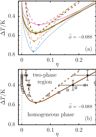
Figure 6: Segregation phase diagram from theory (RPA), experiment, and simulations (MC). (a) The phase diagram obtained within RPA using the four available background potentials $U_{bck}$ from Fig. 5, and their average. The critical Casimir potential is calculated within the Derjaguin approximation using the local functional approach (see Sec. IV.1) for a reduced solvent order parameter $\widetilde{}\phi=-0.088$. The background contributions $U_{bck}$ have been extracted from the experimentally determined effective potentials [compare Eq. (17)] at $\Delta T/\textrm{K}=0.6$ (magenta), $0.5$ (green), $0.4$ (orange), and $0.3$ (blue). The thick dark red curve corresponds to the average of the four potentials $U_{bck}$. The solid lines show the phase boundaries in terms of the packing fraction $\eta$ of the colloids, the dashed lines correspond to the spinodals, and dots represent critical points. (b) Comparison of the theoretical predictions for the phase boundaries (based on the average $U_{bck}$) with Monte Carlo simulations ($\boxdot$) and experiments ($\boldsymbol{\times}$, with error bars) of Ref. Dang et al. (2013). On the temperature axis $\Delta{}T=T_{c}-T$ increases from top to bottom in order to mimic a lower critical point $T_{c}$ (of the solvent) as observed experimentally.

In order to calculate the phase diagram of the effective one-component system within the RPA approximation, we use the pair potential $U\left(r\right)=U_{bck}\left(r\right)+U_{c}\left(r\right)$, where $U_{c}$ is given by Eq. (18), and where the background contribution $U_{bck}$ is extracted from the experimental data of Ref. Dang et al. (2013). As discussed in Sec. IV.1, there is some inaccuracy in determining the background potential $U_{bck}$. Following Ref. Dang et al. (2013) and assuming $\widetilde{}\phi=0$, we have to consider four different $U_{bck}$. The resulting corresponding segregation phase diagrams differ from each other qualitatively. Interestingly, the attractive part of the background potentials $U_{bck}\left(r;\Delta T,\widetilde{}\phi\right)$ corresponding to $\Delta T/\mathrm{K}=0.4$ and $0.2$ [see Fig. 5(a)] is so strong, that for these potentials alone (i.e., for $U=U_{bck}$ without $U_{c}$) the RPA free energy predicts already a phase segregation. For the background potential $U_{bck}\left(r;\Delta T,\widetilde{}\phi\right)$ corresponding to $\Delta T=0.6\mathrm{K}$ and $\widetilde{}\phi=0$, the presence of $U_{c}$ is necessary for the occurrence of phase segregation within RPA. However, the resulting relative value of the critical temperature $(\Delta T)_{c,eff}\simeq 0.39\textrm{K}$ is much smaller than the experimentally observed one. On the other hand, for $\widetilde{}\phi=-0.088$, which renders the best expression for $U_{bck}$ out of the experimental data of Ref. Dang et al. (2013) (see Fig. 5), the resulting RPA phase segregation diagrams are consistent with each other. This is visible in Fig. 6(a), where we compare the coexistence curves $\eta_{cx}\left(T\right)$ resulting from the four potentials $U_{bck}$ of Fig. 5(b), as well as from $U_{bck}$ obtained by averaging these four potentials $U_{bck}$. Although these five background potentials look very similar, they nonetheless lead to coexistence curves the critical temperatures of which differ noticeably [see Fig. 6(a)]. However, away from their critical point, the various coexistence curves merge; see the region $\Delta T<0.4\mathrm{K}$ in Fig. 6(a). This indicates that for small $\Delta T$ the critical Casimir potential dominates the background potential, so that the details of the latter (and thus its inaccuracy) become less important.

Figure 6(b) compares the RPA predictions for the segregation phase diagram with the experimental data and with the Monte Carlo simulation data provided by Ref. Dang et al. (2013). The pair potentials used in these MC simulations are the sum of an attractive and a repulsive exponential function and thus they differ from the ones used here. At high colloidal densities, the RPA is in surprisingly good agreement with the experimental data. On the other hand, at low densities the RPA agrees well with the Monte Carlo simulations, while there both underestimate the experimental values which, in turn, agree well with the RPA-spinodal (an observation also observed for $\widetilde{}\phi=0$). While this latter ‘agreement’ might be accidental, it nevertheless raises the question whether the experimental system has actually been fully equilibrated at the time of the measurements.

V Summary

Critical Casimir forces act between surfaces confining a near-critical medium. For instance, colloidal particles suspended in a binary liquid mixture act as cavities in this solvent. Thus near its critical point of demixing the suspended colloids interact via an effective, solvent-mediated force, the so-called critical Casimir force (CCF). We have analyzed the dependence of the CCFs on the bulk ordering field ($h_{b}$) conjugate to the order parameter of the solvent. For a binary liquid mixture, $h_{b}$ is proportional to the deviation of the difference of the chemical potentials of the two species from its critical value. In the presence of $h_{b}$, we have used mean-field theory to calculate the CCFs between parallel plates and between two spherical colloids, as well as the local functional approach of Fisher and de Gennes for parallel plates. We have shown that the CCF is asymmetric around the consolute point of the solvent, and that it is stronger for compositions slightly poor in that species of the mixture which preferentially adsorbs at the surfaces of the colloids (see Figs. 1, 2(a), 2(b), and 4).

For two three-dimensional spheres posing as hypercylinders $(H_{3,4})$ in spatial dimension $D=4$ we observe a non-monotonic dependence of the scaling function of the CCF on the scaling variable $\Delta=L/R$, where $L$ is the surface-to-surface distance and $R$ is the radius of monodisperse colloids [see Fig. 3(b) as well as Fig. 4]. Unlike four-dimensional spheres ($H_{4,4}$) in $D=4$, the scaling functions for $H_{3,4}$ exhibit a maximum at $\Delta\approx 1/2$ before decreasing upon increasing $\Delta$ [see Fig. 3(b)]. This different behavior may be attributed to the extra macroscopic extension of the hypercylinders $H_{3,4}$. This raises the question whether $H_{3,4}$ or $H_{4,4}$ is the better mean-field approximation for the physically relevant case of three-dimensional spheres $H_{3,3}$ in $D=3$. Due to this uncertainty and also in view of the limited reliability of the Derjaguin approximation (see Figs. 3 and 4) more accurate theoretical approaches are highly desirable. Because the local functional approach is computational less demanding than Monte Carlo simulations and it is reliable for $h_{b}=0$, it would be very useful to improve this approach for $h_{b}\neq 0$ and to generalize it to more complex geometries, in particular to spherical objects.

In addition, due to numerical difficulties the behavior of the scaling function of the CCF for $\Delta\to\infty$ remains as an open issue. Since one faces similar numerical difficulties for $\Delta\to 0$, we conclude that within mean-field theory the numerical solution finds its useful place in between small and large colloid separations. The small separations are captured well by the Derjaguin approximation. For $H_{d,D}$ spheres with $d>\beta D/\nu$, the large separations can be investigated by the so-called small radius expansion. However, the case $H_{3,4}$ represents a ‘marginal’ perturbation for which the small radius expansion is not valid Hanke and Dietrich (1999). Therefore it would be interesting to study the asymptotic behavior of the scaling function of the CCF for large colloid separations by other means.

We have compared our theoretical results for the critical Casimir potential [within the Derjaguin approximation and the local functional approach, see Eq. (18)] with experimental data taken from Ref. Dang et al. (2013) (see Fig. 5). Concerning the potentials we find a fair agreement, however their detailed behavior calls for further, more elaborate experimental and theoretical investigations.

As a consequence of the emergence of CCFs, a colloidal suspension thermodynamically close to the critical point of its solvent undergoes phase separation into a phase dense in colloids and a phase dilute in colloids. Using the random phase approximation for an effective one-component system, we have calculated the phase diagram for this segregation in terms of the colloidal packing fraction and of the deviation of temperature from that of the critical point of the solvent. Surprisingly, despite resorting to these approximations, the calculated phase diagram agrees fairly well with the corresponding experimental and Monte Carlo data (Fig. 6). Both the RPA calculations and the Monte Carlo simulations are based on the so-called effective approach and compare similarly well with the experimental data. However, in order to achieve an even better agreement with the experimental data, it is likely that models have to be considered which take into account the truely ternary character of the colloidal suspension.