Functional renormalization group study of an eight-band model for the iron arsenides

Abstract

We investigate the superconducting pairing instabilities of eight-band models for the iron arsenides. Using a functional renormalization group treatment, we determine how the critical energy scale for superconductivity depends on the electronic band structure. Most importantly, if we vary the parameters from values corresponding to LaFeAsO to SmFeAsO, the pairing scale is strongly enhanced, in accordance with the experimental observation. We analyze the reasons for this trend and compare the results of the eight-band approach to those found using five-band models.

I Introduction

Superconductivity in iron arsenides has been a central field of studies in contemporary solid state physicsPaglione and Greene (2010); Stewart (2011); Hirschfeld et al. (2011); Scalapino (2012); Platt et al. (2013). While many interesting relations and effects have been uncovered, there is still only rudimentary understanding of what should be done to achieve higher transition temperatures exceeding the 55K of SmFeAsOZhi-An et al. (2008). One of the reasons is the complexity of these materials. While DFT techniques can be used to understand the lattice and electronic structure to quite some precisionMazin et al. (2008), our tools for the computation of electronically mediated pairing are still incomplete and will need more refinement to reach predictive power. Furthermore, the many-body calculations that have been performed for these multi-band systems exhibit a rather strong dependence on details of the microscopic Hamiltonian and also on the level of approximations. For example, the dominant pairing state, in particular the competition between $d$-wave and $s^{\pm}$-wave, sensitively depends on the model parametersKuroki et al. (2008); Graser et al. (2009); Chubukov et al. (2009); Thomale et al. (2009, 2011a, 2011b); Platt et al. (2012). While this can reflect the physical reality, one should aim for an understanding of how robust the theoretical results are with respect to the uncertainties of the underlying model and the theoretical approach. This implies testing experimental materials trends against the theoretical picture and also comparing whether different theoretical models arrive at comparable results.

Regarding material trends, a key issue is the systematics of the superconducting $T_{c}$ with the system parameters. Here, the pnictogen height, i.e. the height of the As atom above or below the Fe-planes in FeAs compounds, has been recognized as an important tuning parameter. This was argued by Kuroki et al.Kuroki et al. (2009) in an influential paper already in 2009. These authors showed that the pairing eigenvalues obtained in an RPA treatment of the pairing interaction grow when the pnictogen height is increased. In their 5-band model, the band having iron $d_{X^{2}-Y^{2}}$ $\left(\equiv d_{xy}\right)$ character undergoes strong changes with pnictogen height. When the height is as low as in LaOFeP, the $xy$ hole pocket ceases to exists and is replaced by a $d_{3z^{2}-1}$ pocket. The disappearance of the $d_{xy}$ pocket causes the system to switch from a high-scale pairing phase with a nodeless gap function to a low-scale pairing phase with a very anisotropic gap function, possibly with nodes on the electron pockets. These findingsKuroki et al. (2009) have also been confirmed by other groups, e.g. by using FLEXIkeda et al. (2010) or the functional RGThomale et al. (2011a). For the latter, a consistent picture was provided not only for the superconducting state, but also the change of the magnetic fluctuation profile.

Another possibility to describe the electronic structure of the iron pnictides, is to use an 8-band model which in addition to the 5 iron $d$ orbitals includes 3 pnictide $p$ orbitals. Such a model was worked out by Andersen and BoeriAndersen and Boeri (2011). Whereas in the 5-band description the pnictide $p$-characters are folded into the tails of the $d$-like Wannier orbitals, which thereby become less localized and less $d$-like, the Wannier orbitals in the 8-band description are fairly localized and atomic-like. With that description, one can explicitly see that decreasing the pnictogen height, increases the hopping integral, $t_{xy,z},$ between the pnictide $p_{z}$ and iron $d_{xy}$ orbitals and thereby moves the $pd$ anti-bonding band upwards. Together with this band, the $d_{xy}/p_{z}$-like parts of the electron pockets move and, hence, the Fermi level. Eventually (by LaOFeP) the Fermi level is above the top of the $d_{xy}$ hole pocket which –by being placed at a high-symmetry point– cannot hybridize with the pnictide $p_{z}$ orbital and therefore does not move (with respect to the one-electron potential)Andersen and Boeri (2011).

In the present paper we shall see that although for weakly and optimally electron-doped iron arsenides the $d_{xy}$ hole pocket always exists, the decrease of $p_{z}$-$d_{xy}$ hybridization caused by an increase of the As height (e.g. SmOFeAs) leads to an increase of the pairing scale. This means that the experimentally observed trend may be understood as a change of a single band structure parameter that is most transparently implemented in an 8-band description. More precisely, we shall try to understand the difference between the pairing-energy scales for LaFeAsO, with an experimentalKamihara et al. (2008) $T_{c}$ of $\lesssim 30K,$ and SmFeAsOZhi-An et al. (2008) with $T_{c}\sim 55K,$ i.e. roughly twice as high. These two systems have the same layered, so-called 1111 structure, but the pnictogen height is larger –and the Fe-As tetrahedra closer to being regular– in SmOFeAs than in LaOFeAs. In addition, we shall study the effect of loosing the $d_{xy}$ pocket, as it happens upon overdoping these arsenides.

We do not claim that this more refined effect of the pnictogen height within the five-pocket regime cannot be found in a 5-band description, it is just that it can be obtained very transparently in the 8-band description. Besides exploring the consequences of the variation in pnictogen height, our present 8-band study is also interesting from a methodological point of view. Describing the band structure over a larger energy window should a priori not change the theoretical predictions, but due to the approximations made for the Coulomb correlations, the outcome of 8-band and 5-band calculations can indeed be different. In the usual approximation used for the 5-band model, only the local Coulomb repulsion between the effective Fe $d$ orbitals is considered in terms of density-density and Hund’s rule spin-spin interactions. In $\left(\mathbf{k,}\omega\right)$-orbital-space, this corresponds to a constant interaction. In the 8-band model, however, it is natural to keep also the Coulomb repulsion $U_{pd}$ between Fe $d$ and As $p$ orbitals, thus leading to $\mathbf{k}$-dependent interactions already at the bare level. It may also be worth pointing out, that whereas in the 5-band description, where only the $pd$ antibonding $d$ characters are present, the configuration is $p^{6}d^{6},$ it is $p^{4.5}d^{7.5}$ in the 8-band DFT descriptionSchickling et al. (2012)Haverkort et al. (2012).

Our theoretical approach will be the fRG (functional renormalization group; for recent reviews, see Refs. Metzner et al., 2012; Platt et al., 2013). Such fRG studies have recently been applied to a number of 5-band scenarios. The fRG exhibits similar systematics for the pairing states as the commonly-used RPA and FLEX (fluctuation-exchange approximation)Kuroki et al. (2008); Graser et al. (2009); Ikeda et al. (2010) approaches, but in addition gives reasonable information about the energy scale of the pairing instabilities. In particular, this ansatz allows for a combined DFT-fRG approach, as has been successfully pioneered in the context of LiFeAs where the $s^{\pm}$ SC order prevails as in many other iron-based superconductors despite a significantly deviating magnetic fluctuation profile Platt et al. (2011). The fRG sums all one-loop diagrams to infinite order in the bare interaction. As a subset, it contains the usual ladder sums and RPA summations. These can be understood as geometric series. Hence, the fRG is not biased in favor of one particular kind of ordering. This allows one to obtain tentative phase diagrams having regions with leading antiferromagnetic order bordering superconducting regions.

Here, we shall present a first fRG study of an 8-band model for the iron arsenides. The paper is organized as follows: In Sec. II we describe our model. In Sec. III we give more details about our fRG calculation used to search for superconducting pairing. In Sec. IV we present the relevant fRG results for model parameters corresponding to LaOFeAs, and in Sec. V we show the corresponding data for model parameters adequate for SmOFeAs. In Sec. VI we exhibit and discuss the material trend in terms of the pairing scale when the model parameters are varied continuously from the La- to the Sm situation. We conclude with a discussion of these findings in Sec. VII.

II Model

The starting point for our investigations is the band structure obtained ab-initioAndersen and Boeri (2011) by DFT-GGA calculations for LaOFeAs and presented in the form of the hopping integrals between –and the on-site energies of the 5 Fe $d$ and 3 As $p$ Wannier orbitals (NMTOs). As will be discussed later, we also use ab-initio derived Coulomb interaction parameters. The energy bands with substantial La or O character are more than 2 eV from the Fermi level and are not spanned by our 8-orbital basis set. Only their hybridization with the 8 bands near the Fermi level are included (via the La and O characters downfolded into the tails of the 8 orbitals).

The so-called 1111 structure of LnOFeAs consists of alternating FeAs and LnO layers. The FeAs layer has Fe at the corners of a square lattice with primitive translations $a\mathbf{x}$ and $a\mathbf{y},$ and As alternatively above and below the centers of the squares. The LnO layer has the same structure, but with O substituted for Fe and Ln for As. Due to the above-below alternation of As and Ln, the primitive cell of the translation group contains two LnOFeAs units. However, a single FeAs (or LnOFeAs) layer can be generated by an Abelian group whose elementary operation is a translation $a\mathbf{x}$ or $a\mathbf{y,}$ combined with the $z\rightarrow-z$ reversal (’move one step and stand on your head’)Andersen and Boeri (2011). If one lets the 2D Bloch vector, $\mathbf{k,}$ label the irreducible representations of that group, then the primitive cell contains only one formula unit and the Brillouin zone is a large square with edge $2\pi/a.$ Hopping between FeAs layers, introduces coupling between $\mathbf{k}$ and $\mathbf{k}+\left(\pi,\pi\right)/a$ whereby the BZ is folded into the usual small one, and is given a height $2\pi/c.$ In the LnOFeAs structure the interlayer hopping is mainly between the neighboring As $z$ orbitals and is small for the bands near the Fermi levelAndersen and Boeri (2011). In the present work, interlayer coupling will be neglected, although this is better justified for LaOFeAs than for SmOFeAs, as may be seen from Fig. 9 in Ref. Andersen and Boeri, 2011.

The DFT-GGA-NMTO one-electron Hamiltonian in site and orbital representation is:

$$H_{0}=\sum_{i,j}\sum_{{o,o^{\prime}}\atop{s}}c_{i,o,s}^{\dagger}h_{ij}^{oo^{\prime}}c_{j,o^{\prime},s}\,,$$ (1)

where the $i$ and $j$ run over the square lattice, and $o$ and $o^{\prime}$ over the 8 orbitals. The matrix element $h_{ij^{\prime}}^{oo^{\prime}}$ is the on-site energy of an orbital if $i=j$ and $o=o^{\prime},$ and a hopping integral (or a crystal-field term) if $o\neq o^{\prime}$ or $i\neq j.$ Projecting the Hamiltonian into $\mathbf{k}$-space and diagonalizing the 8$\times$8 matrices for each $\mathbf{k,}$ results in 8 bands and eigenvectors. The overall bandwidth of this 8-band complex is $\sim 7$eV, as can be read off from Fig. 1. In order to use this model for electron-doped LaO_1-xF_xFeAs, we use the rigid band approximation according to which the chemical potential, $\mu,$ is shifted so far upwards with respect to the bands that the growth of the electron pockets plus the shrinkage of the hole pockets amount to $x/2$ times the area of the BZ.

Now, let us discuss the fermiology in more detail (see also Sect. 3.3 in Ref. Andersen and Boeri, 2011). Within the range of relevant dopings, the $e_{g}$-like $\left(d_{x^{2}-y^{2}},d_{3z^{2}-1}\right)$ bands are gapped around the Fermi level, which is therefore crossed by only the $t_{2g}$-like bands. Of these, the $d_{xy}$ band is pure at $\bar{\Gamma}$ $\left(0,0\right)$ –i.e. not hybridizing with any of the other orbitals in the basis set. Because of the glide-mirror symmetry of the Fe-As lattice, the $d_{xy}$ Bloch wave at $k=0$ is out-of-phase on nearest-neighbor Fe sites, i.e. it has anti bonding $dd\pi$ character. Therefore, it forms the top of the band. With the Fermi level a bit lower, this band gives rise to a $\bar{\Gamma}$-centered, nearly circular hole pocket which can be seen in the lower plots of Fig. 1.

Similarly, the $d_{xz}$ and $d_{yz}$ bands are nearly pure at M̄ $\left(\pi,\pi\right),$ where they are degenerate and antibonding $dd\pi.$ The top of the $d_{xz}$ and $d_{yz}$ bands at M̄ are pushed up by weak hybridization with As $p_{x}$ and $p_{y}$ and thus slightly above the top of the $d_{xy}$ band at $\bar{\Gamma}.$ Hence, there are two M̄-centered hole pockets. As seen from the color coding in Fig. 1, the inner pocket has $d_{xz}$ character towards Ȳ $\left(0,\pi\right)$ and $d_{yz}$ character towards X̄ $\left(\pi,0\right),$ while the opposite is true for the outer pocket. Towards $\bar{\Gamma},$ the more dispersing band forming the inner pocket has longitudinal, i.e. $d_{Xz}$ character ($X$ is the $\bar{\Gamma}$M̄ direction) , while the less dispersive band forming the outer pocket has transversal, i.e. $d_{Yz}$ character.

As we move away from its top at $\bar{\Gamma},$ the pure $d_{xy}$ band decreases by about 0.5 eV to minima at X̄ $\left(\pi,0\right)$ and Ȳ $\left(0,\pi\right),$ and towards M̄ it decreases even more, but then hybridizes strongly and looses its $d_{xy}$ character. Starting now from the minima at X̄ and Ȳ, and going towards M̄, hybridization with As $p_{z}$ which increases linearly with the distance from X̄ or Ȳ makes the $d_{xy}/p_{z}$ antibonding band disperse strongly upwards, cross the Fermi level, and near M̄ reach a maximum which in LaOFeAs is more than 1 eV above the Fermi level and in SmOFeAs is $\sim$0.3 eV lower.

Similarly, moving away from the degenerate top at M̄, the nearly pure $d_{xz}$ band decreases slowly towards X̄ where it reaches a minimum merely 0.1 eV below the Fermi level. Going from there towards $\bar{\Gamma}$, hybridization with As $p_{y}$ makes the $d_{xz}/p_{y}$ antibonding band disperse strongly upwards, cross the Fermi level, and reach its maximum at $\bar{\Gamma},$ 2 eV higher. Together with the above-mentioned $d_{xy}/p_{z}$ band, the $d_{xz}/p_{y}$ band forms an X̄-centered electron pocket whose shape is like a super-ellipse pointing towards M̄. The two bands have different minima at X̄ and cross along X̄M̄, because along this line they are not allowed to hybridize with each other. In the lower plots of Fig. 1 we thus see that the X̄-centered electron pocket has predominant $d_{xz}$ character on the long sides, and $d_{xy}$ character along the short sides. Analogously for the Ȳ-centered electron pocket which has $d_{yz}/p_{x}$ character along the long sides and $d_{xy}/p_{z}$ character along the short sides.

The essential difference between the band structures of Sm- and LaOFeAs is that due to the increased As height in Sm, the hopping integral, $t_{xy,z},$ between As $p_{z}$ and Fe $d_{xy}$ is decreased, whereby the antibonding $p_{z}$ bymixing to the $d_{xy}$ band from X̄ or Ȳ and towards M̄ is diminished, and herewith the slope of that band. This makes the electron pockets in Sm- longer –and the Fermi velocity on the short sides lower– than in LaOFeAs. This is illustrated in Fig. 1 and was discussed in Sect. 4.1 of Ref. Andersen and Boeri, 2011.

Andersen and BoeriAndersen and Boeri (2011) noticed that the antibonding $d_{xy}/p_{z}$ band near M̄ causes the dispersion of the inner $d_{xz},d_{yz}$ band to be linear over an energy range which is the larger, the closer the $d_{xy}/p_{z}$ level is to the degenerate $d_{xz},d_{yz}$ level at M̄. The reason is, that the hybridization between $d_{xy}/p_{z}$ and $d_{xz},d_{yz}$ increases linearly with the distance from M̄, so that if the $d_{xy}/p_{z}$ level were degenerate with the $d_{xz},d_{yz}$ level, then the $d_{xy}/p_{z}$ band would form a Dirac cone with one of the $d_{xz},d_{yz}$ bands, which then becomes the inner band. Both for La and SmOFeAs, this linear dispersion extends around the Fermi level. In the present functional RG calculations, no effect of this strong and linear dispersion was found.

Lacking an ab-initio 8-orbital one-electron Hamiltonian for SmOFeAs, we used the one for LaOFeAs and reduced $t_{xy,z}$ from 520 to 325 meV to fit the DFT-GGA-LAPW bandstructure of SmOFeAs. The latter is shown in Fig. 9 of Ref. Andersen and Boeri, 2011 and the result of the model is shown on the upper right-hand side of Fig. 1.

Concerning the Coulomb correlations, we included the density-density terms for the onsite interactions, $U_{dd}$ and $U_{pp},$ between the different $p$ or $d$-orbitals on a given As or Fe-site, as well as the repulsion, $U_{pd},$ between the $d$- and $p$-orbitals on neighboring Fe- and As-sites. In addition, onsite exchange and onsite pair-hopping interactions of the $d$-orbitals were included. The numerical values were taken from cRPA (constrained random phase approximation) studies by Miyake et al.Miyake et al. (2010). They are displayed in Table 1. Rigorously viewed, building the model Hamiltonian from results of two different ab-initio calculations could lead to inconsistencies, but we shall argue in Sect. IV that this does not affect our qualitative results.

By the transformation to the $\left(\mathbf{k},b\right)$-bandrepresentation we get the expression

$$H_{I,\Lambda_{0}}= \frac{1}{N}\sum_{\mathbf{k_{1}},\mathbf{k_{2}},\mathbf{k_{3}}}\sum_{{b_{1},\ldots,b_{4}}\atop{s,s^{\prime}}}V_{\Lambda_{0}}(\mathbf{k_{1}},b_{1};\mathbf{k_{2}},b_{2};\mathbf{k_{3}},b_{3};b_{4})\cdot$$

$$\cdot a_{\mathbf{k_{3}},b_{3},s}^{\dagger}a_{\mathbf{k_{1}}+\mathbf{k_{2}}-\mathbf{k_{3}},b_{4},s^{\prime}}^{\dagger}a_{\mathbf{k_{2}},b_{2},s^{\prime}}a_{\mathbf{k_{1}},b_{1},s}$$ (2)

where the index $\Lambda_{0}$ is used to point out that the electron-electron couplings are the bare ones with respect to our basis. Since we are mainly interested in the consequences of the band structure differences, we first use the LaOFeAs interaction parameters also in the Sm-case, and do some additional checks later on.

$U$	$x^{2}-y^{2}$	$Yz$	$3z^{2}-1$	$Xz$	$xy$
$x^{2}-y^{2}$	$4.66$	$3.09$	$2.99$	$3.09$	$3.57$
$Yz$	$3.09$	$4.08$	$3.31$	$2.90$	$2.91$
$3z^{2}-1$	$2.99$	$3.31$	$4.33$	$3.31$	$2.81$
$Xz$	$3.09$	$2.90$	$3.31$	$4.08$	$2.91$
$xy$	$3.57$	$2.91$	$2.81$	$2.91$	$3.98$
$J$	$x^{2}-y^{2}$	$Yz$	$3z^{2}-1$	$Xz$	$xy$
$x^{2}-y^{2}$		$0.63$	$0.74$	$0.63$	$0.37$
$Yz$	$0.63$		$0.45$	$0.56$	$0.59$
$3z^{2}-1$	$0.74$	$0.45$		$0.45$	$0.67$
$Xz$	$0.63$	$0.56$	$0.45$		$0.59$
$xy$	$0.37$	$0.59$	$0.67$	$0.59$

Table 1: The table shows parameters for onsite interactions of the Fe $d$ orbitals in eV, from Ref. Miyake et al., 2010. Density-density terms are given in the upper half, while the lower half shows the values for exchange interactions. Concerning the onsite density-density interaction of the As $p$ orbitals and nearest neighbor $p$-$d$ repulsion we use the values $U_{pp}=2.6$ eV and $U_{pd}=1.2$ eV.

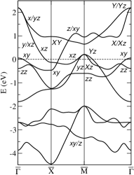
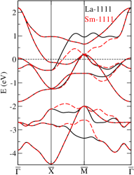
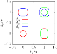
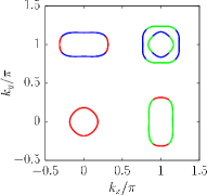
Figure 1: Upper panels: Band structures of La-1111 (left) and Sm-1111 (right) from the 8-band Hamiltonian introduced in the text. On top of the La bands (black) we have plotted the Sm bands (red dashes). Near M̄, at positive energies, the uppermost, $p_{z}$-dominated band of the La band structure moves down in energy and becomes the second-highest band for Sm. Lower panels: Fermi surfaces (La left, Sm right) for the undoped compounds. The color gives the dominant orbital character.

III Functional RG Method

The functional RG approach we use here is basically the same as the one used previously for one-band Hubbard modelsZanchi and Schulz (2000); Halboth and Metzner (2000); Honerkamp et al. (2001) and five-band models for the iron arsenidesWang et al. (2009); Thomale et al. (2011a, b). The underlying formalism and the most important previous applications are discussed in some detail in a recent review by Metzner et al.Metzner et al. (2012) as well as, with a particular emphasis on iron-based superconductors, in a review by Platt et al.Platt et al. (2013). Here we only sketch the main points.

The goal of the fRG approach is to derive an effective low-energy interaction that couples the fermionic degrees of freedom near the Fermi surfaces, say below an energy scale $\Lambda$. This effective interaction should include higher-order corrections due to the excitations at higher energies. These can be included by integrating out the higher-energy modes in the functional integral. In a scheme that is perturbative in the interactions (which should be a reasonable choice for the iron arsenide superconductors) this requires the summation of an infinite number of diagrams. One strength of the RG approach is that it replaces the summation of infinitely many diagrams with all higher-energy modes included by a differential equation whose right hand side contains a handful of second-order diagrams with only modes above an energy scale $\Lambda$ contributing. More precisely, one computes the change of the effective interaction $V_{\Lambda}(\mathbf{k_{1}},b_{1};\mathbf{k_{2}},b_{2};\mathbf{k_{3}},b_{3};b_{4})$ for incoming electrons specified by wave vectors $\mathbf{k_{1}}_{/\mathbf{2}}$ and band indices $b_{1/2}$ and outgoing electrons $\mathbf{k_{3}}_{/\mathbf{4}}$, $b_{3/4}$ (with $\mathbf{k_{4}}$ being fixed by momentum conservation) with decreasing bandwidth $\Lambda$ of the low-energy effective theory, i.e. with successively including the modes with band energies above $\Lambda$. In this notation, spin-rotational invariance is understood and the spin components along the respective quantization axis of particles 1 and 3 and those of 2 and 4 are pairwise identical. The RG equation is then given by

$$\frac{d}{d\Lambda}V_{\Lambda}(\mathbf{k_{1}},b_{1};\mathbf{k_{2}},b_{2};\mathbf{k_{3}},b_{3};b_{4})=\sum_{\mathbf{k},\omega,b,s}V_{\Lambda}\otimes L_{\Lambda}\otimes V_{\Lambda}\,.$$ (3)

In this functional differential equation the summation is over internal quantum numbers (loop variables) $\mathbf{k},\omega,b,s$ for wave vector, Matsubara frequency, band and spin index, and all five one-loop diagrams $L_{\Lambda}$, which are one particle-particle bubble and four different particle-hole diagrams built from two free propagators. The symbols $\otimes$ indicate the convolution of these loop variables with the external variables $\mathbf{k_{1}},b_{1},\mathbf{k_{2}},b_{2},\mathbf{k_{3}},b_{3},b_{4}$ in the arguments of the functions on this right hand side. As we use a momentum-shell cutoff that excludes the modes below scale $\Lambda$, one of the two propagators is at the cutoff energy, i.e. has its absolute value of the band energy, $|\epsilon|$, equal to $\Lambda$, while in the other propagator, the band energy $\epsilon^{\prime}$ fulfills $|\epsilon^{\prime}|\geq\Lambda$. More details can be found in Refs. Metzner et al., 2012; Platt et al., 2013.

Let us also comment on the approximations that go into this fRG scheme. First of all, in the exact hierarchy of flow equations for the one-particle irreducible (1PI) vertex functions, on the right hand side there would be another term representing the impact of the 1PI six-point vertex on the effective interaction (also called 1PI four-point vertex). The 1PI six-point vertex is zero in the bare action but would be generated during the flow. In our truncation we simply drop this term. The impact of the six-point vertex has only been explored recently, and it was found that in simple models it can have at best quantitative but no qualitative effectsMaier and Honerkamp (2012). As the usual Fermi surface instabilities can be understood without these higher order vertices, we think that it is a safe approximation to employ this truncation here. The next and possibly more severe approximation is to drop the self-energy effects on the right hand side of the fRG equation for $V_{\Lambda}$. While the self-energy is definitely very important close to the instability, the accumulated body of experiences for the one-band Hubbard model shows that the leading flows are not altered qualitatively if one includes (parts of) the self-energy feedback. On the other hand, for multi-band systems with multiple Fermi surfaces, the situation could be more difficult, as e.g. small Fermi pockets could be closed already by weaker self-energy effects. The issue of self-energy effects in many-body approaches built on DFT band structures would in addition be overshadowed by the question of a possible double-counting of interaction effects that have already been included in the DFT. This problem must be dealt with in further research. Finally, we also neglect the frequency dependence of the effective interactions. This is again absent in the bare action, unless one would implement the frequency dependence of cRPA interaction parametersAryasetiawan et al. (2004). During the fRG flow, the one-loop diagrams would create a frequency dependence on the interaction on three wavevectors. However, as we are interested in static instabilities at low $T$, we can focus on the flow of the vertices at the smallest fermionic Matsubara frequencies, which go to $0$ as $T\to 0$. Hence in $V_{\Lambda}$ on the left hand side of the flow equation 3, all the fermionic Matsubara frequency are treated as being zero. On the right hand side of 3, the Matsubara sums of the loop diagram still contain two electron propagators whose frequency dependencies are kept. However, since for the vertices we use the zero-frequency values, we can do these sums analytically. Recent fRG studies of the one-band HubbardUebelacker and Honerkamp (2012); Giering and Salmhofer (2012) model take the full frequency dependence of the vertices into account, without major qualitative changes for the context considered here.

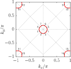
Figure 2: The BZ with two Fermi surface pockets from the same band is divided into $2\cdot m$ patches, with $m=8$ in this example. Every patch contains one patch point on the corresponding Fermi surface.

Besides these simplifications of the fRG equation, we also need an appropriate discretization of the momentum space to be able to integrate this differential equation numerically. For this purpose we use a Fermi surface patching, which was described for the first time by Zanchi and SchulzZanchi and Schulz (2000). Concerning a band that forms at least one Fermi surface, the Brillouin zone is thereby divided into several patches, the number of which is equal to $m$ times the number of Fermi-surface sheets of this band. The arrangement of the patches and corresponding patch points is illustrated in Fig. 2. Now we approximate the interaction to be constant within one patch and use the value at the Fermi surface patch point as a patch value. This approximation can be understood as the mapping

$$V_{\Lambda}(\mathbf{k_{1}},b_{1};\mathbf{k_{2}},b_{2};\mathbf{k_{3}},b_{3};b_{4})\rightarrow V_{\Lambda}(i_{1},i_{2},i_{3},b_{4})\mathnormal{,}$$ (4)

where $i_{j}$ is the patch number corresponding to wave vector $\mathbf{k_{j}}$ and band $b_{j}$. A higher value of $m$ means higher resolution, but also causes higher computational effort. Hence we used $m=16$ as a reasonable compromise for our calculations. The arrangement of the patch points for La-1111 is shown in Fig. 3 in the case of a moderate doped system with five pockets and of a higher doped system where the $d_{xy}$ hole pocket at $\bar{\Gamma}$ is gone. For Sm-1111 this arrangement is very similar to the one shown here. Within this treatment we do not take bands into account that do not cross the Fermi level. This helps to reduce the numerical effort. If such neglected bands are well separated from the Fermi level, this approximation may be very good. If the separation in energy gets small, it can lead to quantitative inaccuracies, especially when there is a band that runs close to the Fermi level without crossing it. The effects of those inaccuracies become evident at some places in our results, as discussed below. For example, the doping-driven transition from a five-pocket to a four-pocket system comes out rather abrupt, while it can be expected to be much smoother in a discretization scheme with a higher resolution of the Brillouin zone and with additional patch points away from the Fermi surface.

Our implementation of the fRG procedure given above is based on one that has been used for previous publications by some of the authors (see e.g. Ref.Thomale et al., 2011a). Besides an extension of the code to eight-orbital/-band systems, we have also implemented improvements concerning some details of the calculation. One detail that should be mentioned here is that the coupling is stored in two different representations during the flow. In addition to the band-dependent effective interaction, $V_{\Lambda}(i_{1},i_{2},i_{3},b_{4})$, we can also transform to the orbital-dependent interaction $V_{\Lambda}(i_{1},i_{2},i_{3},o_{4})$ with an orbital index $o_{4}$ instead of a band index $b_{4}$ on the fourth leg.

Taken together, the fRG in the current setup that is used here contains a number of approximations which could, in bad cases, certainly lead to severe quantitative misestimations of critical scales. On the other hand doing less approximations for multi-band systems will remain difficult for a while, and therefore it is important to learn to what extent the so-obtained information complies with experiments and other methods. In this paper we study whether an experimental $T_{c}$-trend is rendered correctly by the fRG in this form. The result is promising, indicating the possibility that the quantitative artifacts of the approximations are similar for the different systems studied. This provides confidence that the fRG description makes sense and can be extended to other questions.

Before the results for La-1111 and Sm-1111 are shown, we will briefly explain how the renormalized couplings at lower scales can be analyzed. When some values of the effective interaction begin to diverge near a critical scale $\Lambda_{c}$, we have to stop the renormalization and perform a mean-field analysis for the modes below $\Lambda_{c}$. This renormalized mean-field analysis has also been done by Reiss et al.Reiss et al. (2007) in a more complex way and is explained in their paper(see also Refs. Thomale et al., 2009; Platt et al., 2013; Wang et al., 2014 for further examples and developments). In a simple description we can assume that in the case of a leading Cooper instability we can focus on the effective Hamiltonian restricted to the modes below $\Lambda_{c}$

$$H=\sum_{\mathbf{k},s}\epsilon_{\mathbf{k}}a_{\mathbf{k},s}^{\dagger}a_{\mathbf{k},s}+\frac{1}{N}\sum_{\mathbf{k},\mathbf{k^{\prime}}}V_{\mathbf{k},\mathbf{k^{\prime}}}^{\Lambda_{c}}a_{\mathbf{k},\uparrow}^{\dagger}a_{-\mathbf{k},\downarrow}^{\dagger}a_{-\mathbf{k^{\prime}},\downarrow}a_{\mathbf{k^{\prime}},\uparrow}$$ (5)

with $V_{\mathbf{k},\mathbf{k^{\prime}}}^{\Lambda_{c}}=[V_{\Lambda_{c}}(\mathbf{k^{\prime}},-\mathbf{k^{\prime}},\mathbf{k})+V_{\Lambda_{c}}(-\mathbf{k^{\prime}},\mathbf{k^{\prime}},\mathbf{k})]/2$, with the wavevectors in the corresponding bands. By introducing the BCS mean-field $\Delta_{\mathbf{k}}=\frac{1}{N}\sum_{\mathbf{k^{\prime}}}V_{\mathbf{k},\mathbf{k^{\prime}}}^{\Lambda_{c}}\langle a_{-\mathbf{k^{\prime}},\downarrow}a_{\mathbf{k^{\prime}},\uparrow}\rangle$ and neglecting higher order fluctuations the Hamiltonian becomes quadratic whereby it can be diagonalized easily. The value of the gap function has to be calculated self-consistently from the gap equation, which can be simplified to the linearized gap equation

$$\Delta_{\mathbf{k}}=-\frac{1}{N}\sum_{\mathbf{k}^{\prime}}V_{\mathbf{k},\mathbf{k^{\prime}}}^{\Lambda_{c}}\frac{\Delta_{\mathbf{k^{\prime}}}}{2\epsilon_{\mathbf{k^{\prime}}}}\tanh\left(\frac{\epsilon_{\mathbf{k^{\prime}}}}{2T_{c}}\right)$$ (6)

in the limit $T\rightarrow T_{c}$. Now the patch discretization with patches $i$ within which the gap is held constant can be used to simplify this to an eigenvalue problem

$$\eta\Delta_{i}=\sum_{j}V_{i,j}^{\Lambda_{c}}\Delta_{j}$$ (7)

where we have assumed that the integrations within each patch, $-\frac{1}{N}\sum_{\mathbf{k}^{\prime}\in i}\frac{\tanh\left(\frac{\epsilon_{\mathbf{k^{\prime}}}}{2T_{c}}\right)}{2\epsilon_{\mathbf{k^{\prime}}}}\approx-\frac{\rho_{0}}{n}\ln\frac{1.13\Lambda_{c}}{T_{c}}=:\eta^{-1}$, do not depend strongly on the patch index $i$. $\rho_{0}$ is the density of states at the Fermi level, and $n$ is the number of patches. The solution requires that $\Delta_{i}$ is an eigenvector of $V_{i,j}^{\Lambda_{c}}$, with eigenvalue $\lambda=\eta$. The patch dependence of the eigenvector controls the gap form factor, i.e. the angular dependence of the gap. The result for the eigenvalue can be resolved for the critical temperature, yielding

$$T_{c}=1.13\Lambda_{c}\,e^{\frac{n}{\lambda\rho_{0}}}\mathnormal{,}$$ (8)

which is maximal for the lowest (or most negative) eigenvalue. Thus the solution with the lowest eigenvalue characterizes the ground state properties of the system. Note that in this context, the eigenvalue $\lambda$ scales linearly with the patch number. Other instabilities, like the spin-density-wave (SDW), can be analyzed analogously. By comparing the eigenvalues the leading instability can be identified. Moreover, an important implication of the last equation is that the scale $\Lambda_{c}$ is a measure for the critical temperature so that we can use it to compare the transition temperatures of different systems in a simple way.

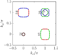
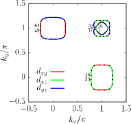
Figure 3: Fermi surface with patch point configuration and numbering for La-1111 with electron doping $x=0.10$ (left) and $x=0.15$ (right).

IV Results for LaOFeAs

First, let us describe the fRG results for the La-1111 parameters. We find flows to strong coupling over a wide parameter range. The leading couplings are either in the SDW channel with wave vector transfer $\sim(\pi,0)$ or in the pairing channel for zero total incoming momentum. In Fig. 4 we plot the critical scale versus doping parameter $x$, together with the information what the leading channel is. For small doping, the SDW instability prevails, while beyond a critical doping the superconducting instability is stronger. The clear separation of these two phases is emphasized by the step in the critical scale which has a similar magnitude as the one found in experiments by Luetkens et al.Luetkens et al. (2009). There is another step in $\Lambda_{c}$ inside the superconducting regime exactly where the hole pocket at $\bar{\Gamma}$ vanishes. It has not been seen in experiments and we have proved that it originates in our implementation at least partially which ignores energy bands not crossing the Fermi level. For this purpose we took into account points for the $\bar{\Gamma}$ band also in the overdoped regime and observed a smoother behavior at the transition from five to four pockets. However, it is clearly physically sound that the loss of a Fermi pocket reduces the pairing scale.

In the superconducting regime we have calculated gap form factors for various dopings by solving the eigenvalue problem (7). This leads to the normal decomposition:

$$V_{i,j}^{\Lambda_{c}}=\sum_{l}\lambda_{l}f_{i}^{\lambda_{l}}f_{j}^{\lambda_{l}}\approx\lambda_{min}f_{i}^{\lambda_{min}}f_{j}^{\lambda_{min}},$$ (9)

in terms of coupling strengths (eigenvalues), $\lambda,$ and form factors (eigenvectors) $\mathbf{f^{\lambda}}$. The last approximation $\approx$ in the equation above keeps only the term from the leading (most negative) eigenvalue. The components $f_{i}^{\lambda_{min}}$ of the corresponding form factor, $\mathbf{f^{\lambda_{\min}},}$ are shown in Fig. 5 and the numbering of the points $i$ running around the Fermi surfaces in Fig. 3. Fig. 5 shows two of these form factors, one for a five-pocket and one for a four-pocket system, where the color indicates the dominant orbital at each patch point on the Fermi surface. Both exhibit a $s^{\pm}$-symmetry and a strong gap anisotropy around the electron pockets, but gap nodes only occur in the four pocket case. All systems studied in the five-pocket regime show a similar form factor to the one shown in the left plot of Fig. 5, and all systems in the four-pocket regime agree qualitatively with the data shown in the right plot. This means that the $\bar{\Gamma}$ pocket is necessary for a diverging $d_{xy}$ interaction, which dominates in the five pocket-systems and leads to high critical scales but is negligible at four pockets. However, as in the case of the critical scale the sudden form factor change between five and four pocket regime is smoothed out by including the $\bar{\Gamma}$ band in the calculations for overdoped systems. When we compare this to previous five-band resultsThomale et al. (2011a), a different anisotropy around the electron pockets is striking in the five pocket model for La-1111. In these older findings the dominant interactions had $d_{xz}$ and $d_{yz}$ character, which resulted in an inverted anisotropy compared to the one shown here. In contrast, the form factors of the four-pocket systems are very similar. Since the interactions that involve $p$-orbitals are not taken into account explicitly in five-band studies, we analyze the effect of the initial interactions of this kind on our system. It becomes apparent that the dominance of the $d_{xy}$-orbital in the form factor for the five-pocket systems is reduced when one neglects initial $p$-$d$ interactions. This behavior suggests that the difference in the gap anisotropy between the five- and eight-band results is systematic due to downfolding on distinct basis sets. The orbital composition of the superconducting pairing can hardly be measured, but the differences in orbital composition of the pairing changes the gap anisotropy quantitatively, which is a measurable effect. Note that in case of a dominant $d_{xy}$ pocket, the gap minima on the electron pockets appear on the long sides, while in the five-band studies, they are located on the short sidesThomale et al. (2011a). We have checked that is difference not simply matter of slightly different parameters for the two models. By reducing the relative strength of the $U_{xy,xy}$-interaction parameter compared to the other $U$s, we can tune the five-pocket case in the eight-band model to give gap structures analogous to the five-band results, but we have to change these interaction parameters substantially for this.

In order to get more insight into the structure of the renormalized couplings, we transform Eq. (7) from band to orbital space and diagonalize the matrix of pairing interactions between Fermi-surface patches. Now we can clearly see what was mentioned above: When the $d_{xy}$ hole pocket is present, the pairing interactions between Fermi-surface points with prevailing $d_{xy}$ character dominate and the gap minima on the electron pockets appear on the long sides where the X̄ pocket has $d_{xz}$ and the Ȳ pocket $d_{yx}$ character. When the $d_{xy}$ hole pocket is doped away and $d_{xy}$ character only remains on the short sides of the electron pockets, the pairing interactions among $\mathbf{k}$-points with prevailing $d_{xz}$ or $d_{yz}$ character dominate and the gap minima on the electron pockets appear on the short sides where the character is $d_{xy}.$

Another interesting aspect is the sign structure of the form factors, which supports the often stated $s^{\pm}$ symmetry. Note that in our formalism, the signs of the coupling components in band representation are not necessarily meaningful since they result from the choice of the arbitrary signs in the transformation matrices from orbital to band picture. Transformation to the orbital basis removes this ambiguity. With the transformation chosen here, the sign structure of the gap turns out to be the same, both in band picture as well as in the orbital basis. This confirms the stated $s^{\pm}$ symmetry unambiguously.

Hence we conclude this comparison of the eight-band results with previous five-band studies with the statement that the two models and their fRG-implementations agree on the sign-changing $s$-wave pairing, but that different gap anisotropies are possible. Different models have somewhat different parameter regimes with respect to the leading orbital in the pairing and the location of the gap minima.

Next let us discuss the issue of combining results of two different ab-initio calculations (one for the dispersion, one for the interaction parameters) to build up our model. For this purpose we have changed the initial interactions to analyze the stability of our results against details of these values. More precisely we have added prefactors to some interaction parameters $U_{\mu,\mu^{\prime}}\rightarrow f\cdot U_{\mu,\mu^{\prime}}$ in order to tune these values. We have varied a) the $pd$-interaction with $\mu\in d$-orbitals and $\mu^{\prime}\in p$-orbitals, and b) the onsite $dd$-interaction of the $\mu=\mu^{\prime}=d_{xy}$-orbital. The latter one is known vary most between different iron pnictide superconductors, according to cRPA-calculationsMiyake et al. (2010) that determine the effective interaction parameters for the model considered. In both cases the resulting form factors have shown only a marginal dependence on this prefactor. As shown in Fig. 6 the critical scales are affected by changing these prefactors, but their orders of magnitude not. In other words our, qualitative results do not depend strongly on the details of the initial interaction parameters. Thus, we think it is justified to use the above given ab-initio model. Regarding the effect of the $U_{pd}$ interaction, we have varied this value between $-50\%$ and $+150\%$ of the values listed in Miyake et al., 2010 and found a monotonous trend. This shows that a positive $U_{pd}$ enhances the pairing scale, and mainly enforces the pairing within the $d_{xy}$-dominated parts.

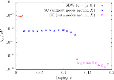
Figure 4: FRG phase diagram for La-1111. The colors or symbols indicate the leading instability at a given electron doping.

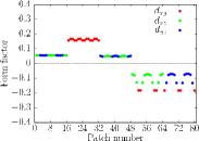
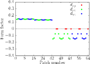
Figure 5: FRG form factors of the superconducting gap for La-1111 at electron dopings $x=0.10$ (left) and $x=0.15$ (right) calculated from the linearized gap equation.

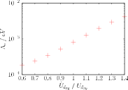
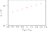
Figure 6: The critical scales are plotted against varied initial interaction parameters $U_{\mu,\mu^{\prime}}\rightarrow\tilde{U}_{\mu,\mu^{\prime}}=f\cdot U_{\mu,\mu^{\prime}}$ with $\mu=\mu^{\prime}=d_{xy}$ (left) or $\mu\in d$-orbitals and $\mu^{\prime}\in p$-orbitals (right).

V Results for SmOFeAs

In this part of the paper the fRG results for the Sm-1111 model are presented and compared with those for La-1111. Here again, we find two competing instabilities in the investigated range of electron dopings. In contrast to the phase diagram for La-1111, the data for Sm-1111 in Fig. 7 do not exhibit a step in the divergence scale between the transition from the SDW to the SC phase. Furthermore, this transition is not sharp for Sm-1111, but there is a region in which the dominant instability cannot be determined unambiguously. Our findings are consistent with the experimental results of Drew et al.Drew et al. (2009) which also exhibit a transition between a magnetic and a superconducting phase with continuous $T_{c}$ behavior. The absolute pairing scales in Sm-1111 from Fig. 7 are about three to four times as high as the ones for La-1111 from Fig. 4 in the SC region, while they are similar in the SDW region. This interesting parameter trend which agrees with the experimental $T_{c}$s will be discussed further in the next chapter.

Like in La-1111, the superconducting form factors shown in Fig. 8 have $s^{\pm}$-symmetry and depend mainly on whether the $d_{xy}$ pocket exists or not. In the overdoped, four-pocket regime the form factors with nodes on the short, $d_{xy}$-dominated sides of the electron pockets, are nearly identical in the two materials. In the optimally doped, five-pocket regime, the gap anisotropy on the electron pockets is far less pronounced in Sm-1111 and the position of the smallest gap has changed on the long sides of the electron pockets. That the gap on the electron pockets is far more isotropic in optimally doped Sm-1111 than in La, should be experimentally observable.

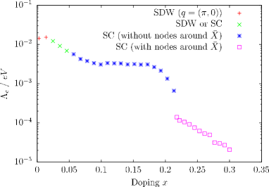
Figure 7: FRG phase diagram for Sm-1111. The colors or symbols indicate the leading instability at a given doping.

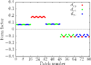
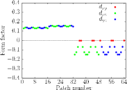
Figure 8: FRG form factors of the superconducting gap for Sm-1111 at dopings $x=0.19$ (left) and $x=0.25$ (right) calculated from the linearized gap equation.

VI Material trend from LaFeAsO to SmFeAsO

We now concentrate on the calculated material-dependent critical scales in the superconducting five-pocket regime. Our trend seems to be consistent with the experimental observation that Sm-1111 has far higher critical temperatures than La-1111. We shall distinguish between two different effects of tuning the hopping integral $t_{xy,z}$ from its value (520 meV) in La to the one (325 meV) in Sm, which could be responsible for the above-mentioned material trend. The first effect stems from the change of the eigenvectors of the Hamiltonian (1), i.e. of the orbital characters on the Fermi surface. These orbital characters enter the FRG flow via the initial conditions for the interactions expressed in the band picture. This means that the wavevector-dependence of the initial interaction depends on the tuning parameter $t_{xy,z}$. The second place where the tuning parameter enters is the band energies, with direct impact on the shape of the Fermi surface and the Fermi velocities.

To analyze the effect of the orbital composition in the initial interaction, we have tuned the system from La to Sm using the varying orbital-band transformation, but keeping the La band structure, i.e. keeping the Fermi surfaces unchanged. Fig. 9 shows that the orbital composition influences the critical scales, but cannot be responsible for the higher scales in Sm because the trend is more or less opposite. The discontinuity in the data in this case is presumably an artifact of the $N$-patch discretization (a near band crossing). For a better $\mathbf{k}$-discretization, this step should be smoothened out.

In order to investigate the effect changing the band dispersions, we have chosen ’averaged’ initial interactions that do not depend on the band or on the wavevectors and then varied the band energies and the Fermi surfaces via $t_{xy,z}$. The resulting critical scales are shown in Fig. 10 with three different average initial coupling values. Here we see that the change of Fermi-surface shape and velocities leads to increasing critical scales along the way from La to Sm. Hence the material trend seems to be an effect of the band dispersion.

The simplest attempt to interpret the effect of the dispersion may be to consider it as a density-of-states effect. We have calculated the density of states at the Fermi level in La-1111 as well as in Sm-1111 for the various parameters under consideration. The result is that it is higher for Sm-1111 due to the flattening of the $d_{xy}/p_{z}$ band forming the short sides of the electron pockets. On first sight, this seems to be consistent with the higher scales in the superconducting regime. However, this would also suggest higher scales in the SDW phase, in contradiction to our fRG findings, and also in contradiction to the experimental findingsZhi-An et al. (2008). So the density of states at the Fermi level appears to be too simple to give a sufficient explanation.

Next, we have computed the corresponding particle-hole diagrams at the spin-density wave ordering vector and particle-particle diagrams at zero total momentum. They sample the dispersion over a wider energy range than the above-used density of states, which is only a measure at the Fermi level. For Sm-1111, both bubbles at these specific wave-vectors become larger by a few percent in very similar way. So, naively, both pairing and SDW scale should go up. In the fRG the larger SDW tendency due to a larger value of the particle-hole diagram could be compensated by a stronger screening of the repulsions in the likewise strengthened pairing channel. Yet, this does not help to understand in simple why the pairing scale still manages to gain from the change in the band structure.

Of greater significance might be that the increased elongation of the Sm electron pockets caused by the flattening of the $d_{xy}/p_{z}$ band, spreads out the $\left(\pi,0\right)$ and $\left(0,\pi\right)$ susceptibility peaks. Indeed, by looking at the wavevector-dependence of the particle-hole bubble that determines the bare spin susceptibility, it becomes apparent that its peak not only becomes higher at the SDW ordering wavevector when going from La-1111 to Sm-1111, but it also becomes broader. We can use this susceptibility as pairing interaction in the BCS gap equation. Then the wavevector summation in the gap equation samples the whole neighborhood of the SDW peak, and one might hope that the broadening of the peak might help to understand the rise in the pairing scale. We have computed the pairing eigenvalues with the bare susceptibility as pairing interaction in the BCS gap equation. However, we found that the analysis of the parameter trend from La-1111 to Sm-1111 is severely disturbed by a number of competing pairing channels known from previous studiesGraser et al. (2009) that do not get removed unless we do a more sophisticated summation of many diagrams, as is ultimately done in the fRG.

Hence, we are led to the conclusion that it is rather difficult to use single-channel or low-order considerations for the explanation of the material trend from Sm-1111 to La-1111 seen in the fRG. A combined treatment of all fluctuations channels to high orders such as in the fRG appears to be vital to capture this trend.

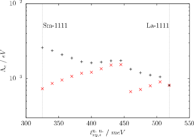
Figure 9: Black crosses: Critical pairing scales of La-1111, Sm-1111 and fictitious intermediate systems versus the band-structure tuning parameter, $t_{xy,z},$ at a chemical potential of $\mu=45\ \textnormal{meV}$, corresponding to $x=0.10$ in La-1111. For comparison, with red crosses we show the critical scales of fictitious systems whose dispersions are fixed to the La-1111 bands, but whose composition of interactions changes according to the changing orbital character of the true $t_{xy,z},$-dependent bands.

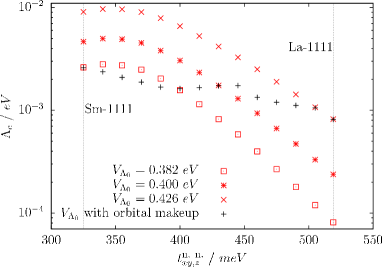
Figure 10: Same as Fig. 9, except that the red symbols are now for systems whose band structures vary with $t_{xy,z},$ but have initial couplings, $V_{\Lambda_{0}},$ fixed to wavevector and bandindex independent values that are $382$, $400$ or $426$ meV.

VII Discussion

We have performed extended fRG calculations for a two-dimensional eight-band model for 1111 iron arsenides. The fRG goes beyond RPA-type many-body approaches, and has until now only been applied to five-band models for the iron superconductors. Our study shows that in the eight-band model, the primary instabilities toward antiferromagnetic SDW and sign-changing $s$-wave pairing are reproduced clearly. However, regarding the question which orbitals contribute most to the pairing, we found some model dependencies. In the eight-band $pd$ model with two electron and three hole pockets, the $d_{xy}$ hole pocket plays a more important role for pairing than in corresponding five-band $d$-only models. This also qualitatively changes the gap anisotropy on the electron pockets. In the eight-band model, the gap minima on these pockets appear on the long rather than on the short sides. This difference should be experimentally accessible. At present, we regard these differences as an indication of how approximate many-body treatments of these complicated multi-band models currently are. Future theoretical work must find ways to understand and reduce the model-dependence of the theoretical results. On the positive side, we have seen that besides the $d_{xz/yz}$-dominated pairing found in five-band studies, also the second plausible scenario, the $d_{xy}$-dominated pairing is theoretically possible.

We have used the hopping integral $t_{xy,z}$ between the Fe $d_{xy}$ and the As $p_{z}$ orbital to tune the eight-band model derived for La-1111 ($T_{c}\lesssim 29\,$K) to the one appropriate for Sm-1111 ($T_{c}\sim 50\,$K)Andersen and Boeri (2011). Upon this tuning, our theoretical estimate for the pairing temperature, the calculated scale of divergence for the fRG flow, increases by a factor $\sim 3.$ In contrast with this, the energy scale for SDW ordering for the undoped systems is only slightly increased. These differences between the two systems are in qualitative agreement with the experimental phase diagrams. It also agrees with previous worksKuroki et al. (2009) which showed that regular tetrahedra have the highest superconducting energy scale. This structural change is the main cause for the variation of the tuning parameter. However, besides being able two make the system switch from a high-pairing-scale five-pocket regime to a low-pairing-scale four-pocket regime as previously pointed outKuroki et al. (2009); Ikeda et al. (2010); Thomale et al. (2011a), the tuning parameter also causes a distinct and relevant trend within the five-pocket regime. Hence our study reveals a major simplification regarding the modeling of the materials: it shows that in the 8-band description the change of the pairing scale over 5- and 4-pocket regime can be described by adjusting a single parameter besides the band filling.

We have mentioned that simple measures like the density of states at the Fermi level, or the values of one-loop diagrams, do not allow one to understand the band-structure effects on the pairing scale in simple terms. On the other hand, we have seen that the effect correlates positively with the change of the Fermi-surface shape and velocities, but less with the change of the orbital composition of the Fermi surface. The difficulty in identifying a simple reason for the increase of the critical scales mainly points to the complexity of the interplay of spin- and pairing fluctuations in such multi-band systems. Nevertheless, we can associate the scale-increase for the superconducting pairing with a single band structure parameter, whose behavior can be understood from the structural change, namely the pnictogen height.

In our view, these results and other previous worksKuroki et al. (2009); Wang et al. (2010); Andersen and Boeri (2011); Thomale et al. (2011a), on material trends on iron-arsenide models are the first steps towards a more ambitious program of correlating theoretical results on different iron arsenide systems with non-universal experimental findings. This serves two goals: first this research helps us to understand how quantitative and how robust our present treatments of the many-body physics in these systems are, and second the so-obtained understanding may be very useful for the development of materials with deliberately tailored, superior properties.

References

- Paglione and Greene (2010) J. Paglione and R. L. Greene, Nature Physics 6, 645 (2010).
- Stewart (2011) G. R. Stewart, Rev. Mod. Phys. 83, 1589 (2011).
- Hirschfeld et al. (2011) P. J. Hirschfeld, M. M. Korshunov, and I. I. Mazin, Reports on Progress in Physics 74, 124508 (2011).
- Scalapino (2012) D. J. Scalapino, Rev. Mod. Phys. 84, 1383 (2012).
- Platt et al. (2013) C. Platt, W. Hanke, and R. Thomale, Adv. Phys. 62, 453 (2013).
- Zhi-An et al. (2008) R. Zhi-An, L. Wei, Y. Jie, Y. Wei, S. Xiao-Li, Zheng-Cai, C. Guang-Can, D. Xiao-Li, S. Li-Ling, Z. Fang, and Z. Zhong-Xian, Chinese Physics Letters 25, 2215 (2008).
- Mazin et al. (2008) I. I. Mazin, M. D. Johannes, L. Boeri, K. Koepernik, and D. J. Singh, Phys. Rev. B 78, 085104 (2008).
- Kuroki et al. (2008) K. Kuroki, S. Onari, R. Arita, H. Usui, Y. Tanaka, H. Kontani, and H. Aoki, Phys. Rev. Lett. 101, 087004 (2008).
- Graser et al. (2009) S. Graser, T. A. Maier, P. J. Hirschfeld, and D. J. Scalapino, New Journal of Physics 11, 025016 (2009).
- Chubukov et al. (2009) A. V. Chubukov, M. G. Vavilov, and A. B. Vorontsov, Phys. Rev. B 80, 140515 (2009).
- Thomale et al. (2009) R. Thomale, C. Platt, J. Hu, C. Honerkamp, and B. A. Bernevig, Phys. Rev. B 80, 180505 (2009).
- Thomale et al. (2011a) R. Thomale, C. Platt, W. Hanke, and B. A. Bernevig, Phys. Rev. Lett. 106, 187003 (2011a).
- Thomale et al. (2011b) R. Thomale, C. Platt, W. Hanke, J. Hu, and B. A. Bernevig, Phys. Rev. Lett. 107, 117001 (2011b).
- Platt et al. (2012) C. Platt, R. Thomale, C. Honerkamp, S.-C. Zhang, and W. Hanke, Phys. Rev. B 85, 180502 (2012).
- Kuroki et al. (2009) K. Kuroki, H. Usui, S. Onari, R. Arita, and H. Aoki, Phys. Rev. B 79, 224511 (2009).
- Note (1) Kuroki et al. Kuroki et al. (2009) have the pocket at while we have it at . Similarly, Kuroki et al. have the two other hole pockets at while we have them at . The reason is given in Fig. 3 of Ref Andersen and Boeri, 2011. In general, the pseudo-momentum used by Kuroki et al. differs by from our -vector which enumerates the irreducible representations of the Abelian group generated by the glide-mirror operation Lee and Wen (2008).
- Ikeda et al. (2010) H. Ikeda, R. Arita, and J. Kuneš, Phys. Rev. B 81, 054502 (2010).
- Andersen and Boeri (2011) O. Andersen and L. Boeri, Annalen der Physik 523, 8 (2011).
- Kamihara et al. (2008) Y. Kamihara, T. Watanabe, M. Hirano, and H. Hosono, Journal of the American Chemical Society 130, 3296 (2008), http://pubs.acs.org/doi/pdf/10.1021/ja800073m .
- Schickling et al. (2012) T. Schickling, F. Gebhard, J. Bünemann, L. Boeri, O. K. Andersen, and W. Weber, Phys. Rev. Lett. 108, 036406 (2012).
- Haverkort et al. (2012) M. W. Haverkort, M. Zwierzycki, and O. K. Andersen, Phys. Rev. B 85, 165113 (2012).
- Metzner et al. (2012) W. Metzner, M. Salmhofer, C. Honerkamp, V. Meden, and K. Schönhammer, Rev. Mod. Phys. 84, 299 (2012).
- Platt et al. (2011) C. Platt, R. Thomale, and W. Hanke, Phys. Rev. B 84, 235121 (2011).
- Note (2) The 5-set (and the 8-set) Wannier orbitals are generated in the tetragonal -system and then linear combined to the cubic system, e.g.: Due to the tails on As, those linear combinations are not simply 45∘ rotations (see Fig. 5 in Ref. Andersen and Boeri, 2011).
- Note (3) The “cubic” and axes point from Fe to the nearest Fe neighbors on the square lattice, while the “tetragonal” and axes are turned by 45∘ and point towards the projection of the pnictide onto the Fe plane. .
- Miyake et al. (2010) T. Miyake, K. Nakamura, R. Arita, and M. Imada, Journal of the Physical Society of Japan 79, 044705 (2010).
- Zanchi and Schulz (2000) D. Zanchi and H. J. Schulz, Phys. Rev. B 61, 13609 (2000).
- Halboth and Metzner (2000) C. J. Halboth and W. Metzner, Phys. Rev. B 61, 7364 (2000).
- Honerkamp et al. (2001) C. Honerkamp, M. Salmhofer, N. Furukawa, and T. M. Rice, Phys. Rev. B 63, 035109 (2001).
- Wang et al. (2009) F. Wang, H. Zhai, Y. Ran, A. Vishwanath, and D.-H. Lee, Phys. Rev. Lett. 102, 047005 (2009).
- Maier and Honerkamp (2012) S. A. Maier and C. Honerkamp, Phys. Rev. B 85, 064520 (2012).
- Aryasetiawan et al. (2004) F. Aryasetiawan, M. Imada, A. Georges, G. Kotliar, S. Biermann, and A. I. Lichtenstein, Phys. Rev. B 70, 195104 (2004).
- Uebelacker and Honerkamp (2012) S. Uebelacker and C. Honerkamp, Phys. Rev. B 86, 235140 (2012).
- Giering and Salmhofer (2012) K.-U. Giering and M. Salmhofer, Phys. Rev. B 86, 245122 (2012).
- Reiss et al. (2007) J. Reiss, D. Rohe, and W. Metzner, Phys. Rev. B 75, 075110 (2007).
- Wang et al. (2014) J. Wang, A. Eberlein, and W. Metzner, Phys. Rev. B 89, 121116 (2014).
- Luetkens et al. (2009) H. Luetkens, H.-H. Klauss, M. Kraken, F. J. Litterst, T. Dellmann, R. Klingeler, C. Hess, R. Khasanov, A. Amato, C. Baines, M. Kosmala, O. J. Schumann, M. Braden, J. Hamann-Borrero, N. Leps, A. Kondrat, G. Behr, J. Werner, and B. Büchner, Nature Materials 8, 305 (2009), arXiv:0806.3533 [cond-mat.supr-con] .
- Drew et al. (2009) A. J. Drew, C. Niedermayer, P. J. Baker, F. L. Pratt, S. J. Blundell, T. Lancaster, R. H. Liu, G. Wu, X. H. Chen, I. Watanabe, V. K. Malik, A. Dubroka, M. Rössle, K. W. Kim, C. Baines, and C. Bernhard, Nature Materials 8, 310 (2009), arXiv:0807.4876 [cond-mat.supr-con] .
- Wang et al. (2010) F. Wang, H. Zhai, and D.-H. Lee, Phys. Rev. B 81, 184512 (2010).
- Lee and Wen (2008) P. A. Lee and X.-G. Wen, Phys. Rev. B 78, 144517 (2008).