On efficient dimension reduction with respect to a statistical functional of interest

Abstract

We introduce a new sufficient dimension reduction framework that targets a statistical functional of interest, and propose an efficient estimator for the semiparametric estimation problems of this type. The statistical functional covers a wide range of applications, such as conditional mean, conditional variance and conditional quantile. We derive the general forms of the efficient score and efficient information as well as their specific forms for three important statistical functionals: the linear functional, the composite linear functional and the implicit functional. In conjunction with our theoretical analysis, we also propose a class of one-step Newton–Raphson estimators and show by simulations that they substantially outperform existing methods. Finally, we apply the new method to construct the central mean and central variance subspaces for a data set involving the physical measurements and age of abalones, which exhibits a strong pattern of heteroscedasticity.

On efficient dimension reduction with respect to a statistical functional of interest

, and t1Supported in part by a NSF Grant DMS-11-06815. t2Supported in part by a NSF Grant DMS-12-05546.

62-09, 62G99, 62H99, Central subspace, conditional mean, variance and quantile, efficient information, efficient score, Frechet derivative and its representation, projection, tangent space

1 Introduction

The purpose of this paper is twofold: to introduce a new framework for sufficient dimension reduction that targets a statistical functional of interest, and to develop semiparametrically efficient estimators for problems of this type.

Let $X$ be a $p$-dimensional random vector and $Y$ be a random variable. In classical sufficient dimension reduction (SDR), we are interested in a lower dimensional linear predictor $\zeta^{\mathsf{T}}X$, where $\zeta$ is a $p\times d$ matrix with $d<p$, such that $Y$ is independent of $X$ given $\zeta^{\mathsf{T}}X$. That is, the conditional distribution of $Y$ given $X$ is the same as that of $Y$ given $\zeta^{\mathsf{T}}X$. In this problem, the identifiable parameter is $\operatorname{span}(\zeta)$, the subspace of $\mathbb{R}^{p}$ spanned by the columns of $\zeta$. Under mild conditions, there exists a unique smallest subspace that satisfies this condition, and it is called the central subspace; see Li (1991, 1992), Cook and Weisberg (1991), Cook (1994, 1996, 1998). For a general discussion of the sufficient conditions for the central subspace to exist, see Yin, Li and Cook (2008). The SDR  provides us a mechanism to reduce the dimension of the predictor while preserving the conditional distribution of $Y$ given $X$.

In many applications, our interests are in some specific aspects of the conditional distribution $P_{Y|X}$. For example, in nonparametric regression, we are interested in the conditional mean $E(Y|X)$; in median regression, we are interested in the conditional median $M(Y|X)$, and in volatility analysis we are interested in the conditional variance $\operatorname{Var}(Y|X)$ and in supervised classification we are interested in the class label of $Y$ given its covariates $X$. To illuminate this point further, let us consider the model

$$Y=\mu(X_{1})+\sigma(X_{1}+X_{2})\varepsilon,$$ (1)

where $\mu$ and $\sigma$ are unknown functions. In this case, the central subspace, which is the two-dimensional subspace of $\mathbb{R}^{p}$ spanned by $(1,0,\ldots,0)$ and $(0,1,0,\ldots,0)$, only tells us the sufficient predictors can be any linear combination of $X_{1}$ and $X_{2}$, but it does not tell us that the conditional mean is a function of $X_{1}$, and the conditional variance is a function of $X_{1}+X_{2}$. Thus, the information provided by the central subspace is clearly inadequate if we want to build a model like (1).

Under these circumstances, it makes sense to reformulate sufficient dimension reduction to target a specific functional, so as to provide a more nuanced picture of the relation between $X$ and $Y$ than offered by the central subspace. Several such efforts have been made over the past decade or so. For example, Cook and Li (2002) introduced the central mean subspace, which is defined by the relation $E(Y|X)=E(Y|\alpha^{\mathsf{T}}X)$, where $\alpha$ is minimal in the same sense as it is in the central subspace. Yin and Cook (2002) introduced the $k$th central moment subspace through the relation $E(Y^{k}|X)=E(Y^{k}|\alpha^{\mathsf{T}}X)$. Zhu and Zhu (2009) introduced the central variance subspace by requiring that $\operatorname{Var}(Y|X)$ is a function of $\alpha^{\mathsf{T}}X$. Zhu, Dong and Li (2013) introduced a general class of estimating equations for single-index conditional variance. The Minimum Average Variance Estimator (MAVE) by Xia et al. (2002) also targets the central mean subspace. Kong and Xia (2012) introduced an adaptive quantile estimator for single-index quantile regression, which targets the conditional quantile. It turns out the space spanned by the columns of $\alpha$ in the above relations are all subspaces of the central subspace. They provide refined structures for the central subspace. As a consequence, $\alpha^{\mathsf{T}}X$ can be written as $\beta^{\mathsf{T}}\zeta^{\mathsf{T}}X$, and we can refine central subspace based on the sufficient predictor $\zeta^{\mathsf{T}}X$. For convenience, we reset $\zeta^{\mathsf{T}}X$ as $X$, and use $\tilde{X}$ to represent the original predictor throughout the rest of the paper.

The first goal of this paper is to unify these problems by introducing a general dimension reduction paradigm with respect to statistical functional $T$ of the conditional density of $Y$ given $X$, say $\eta(x,y)$, through the following statement:

$$T\bigl{(}\eta(x,\cdot)\bigr{)}\mbox{ is a function of $\beta^{\mathsf{T}}x$}.$$ (2)

Note that sufficient dimension reduction for conditional mean, conditional moments and conditional variance discussed in the last paragraph are all special cases of relation (2). The minimal subspace $\operatorname{span}(\beta)$ of $\mathbb{R}^{p}$ that satisfies this relation is called the $T$-central subspace.

The second, and the main goal of this paper is to develop semiparametrically efficient estimators for the $T$-central subspace. In a series of recent papers, Ma and Zhu (2012, 2013a, 2013b) use semiparametric theory to study sufficient dimension reduction and develop semiparametrically efficient estimators of the central subspace. These are related to the earlier developments by Li and Dong (2009) and Dong and Li (2010), which use estimating equations to relax the elliptical distribution assumption for sufficient dimension reduction. We extend Ma and Zhu’s approach to find semiparametrically efficient estimator for the $T$-central subspace. We derive the general formulas for the efficient score and efficient information for the semiparametric family specified by the relation (2), and further deduce their specific forms for three important statistical functionals: the linear functionals (L-functionals), the composite linear functionals (C-functionals) and implicit functionals (I-functionals). These functionals cover a wide range of applications. For example, all conditional moments are L-functionals, all conditional cumulants [see, e.g., McCullagh (1987)] are C-functionals and quantities such as conditional median, conditional quantile and conditional support vector machine Li, Artemiou and Li (2011) are I-functionals.

Using the formulas for efficient score and efficient information, we propose a one-step Newton–Raphson alorithm to implement semiparametrically efficient estimation. Compared with the semiparametric estimators of Ma and Zhu (2013a), our algorithm has two distinct and attractive features. First, since our algorithm relies on the MAVE-type procedure for minimization, it can be implemented by iterations of a least squares problem without resorting to high-dimensional search-based optimization. Second, unlike Ma and Zhu (2013a), our method does not require any specific parameterization of $\beta$ that potentially restricts the generality of their method.

The rest of the paper is organized as follows. In Section 2, we give a general formulation of sufficient dimension reduction with respect to a statistical functional of interest. To set the stage for further development, we lay out the semiparametric structure of our problem in Section 3. In Section 4, we derive the efficient score and efficient information for a general statistical functional. In Sections 5, 6 and 7, we further deduce the specific forms of the efficient score and efficient information for the L-, C- and I-functionals. In Section 8, we discuss the effect of estimating the central subspace on the efficient score. In Section 9, we develop the one-step Newton–Raphson estimation procedure for semiparametrically efficient estimation. In Section 10, we conduct simulation studies to compare our method with other methods, and in Section 11 we apply our method to a data set. Some concluding remarks are made in Section 12. The proofs of some technical results are given in the supplementary material [Luo, Li and Yin (2014)].

The following notation will be consistently used throughout the rest of the paper. The symbol $I_{k}$ denotes the $k\times k$ dimensional identity matrix; $e_{k}$ denotes a vector whose $k$th entry is 1 and other entries are 0; $\perp\!\!\!\!\perp$ indicates independence or conditional independence between two random elements—that is, $A\perp\!\!\!\!\perp B$ means $A$ and $B$ are independent, and $A\perp\!\!\!\!\perp B|C$ means $A$ and $B$ are independent given $C$. For integers $s$ and $t$, $\mathbb{R}^{s}$ denotes the $s$ dimensional Euclidean space, and $\mathbb{R}^{s\times t}$ denotes the set of $s\times t$ dimensional matrices. For a function with multiple arguments, say $f(x,y,z)$, we use the dot notation to represent mappings of a subset of the arguments. For example, $f(\cdot,y,z)$ represents the mapping $x\mapsto f(x,y,z)$ where $y$ and $z$ are fixed, and $f(\cdot,\cdot,z)$ represents the mapping $(x,y)\mapsto f(x,y,z)$ where $z$ is fixed. We use superscripts of $X$ to index components and subscripts of $X$ to index subjects. Thus, $X_{i}^{j}$ means the $j$th component of the $i$th observation in a sample $X_{1},\ldots,X_{n}$. However, $a^{i}$ represents power when $a$ is not $X$.

2 Dimension reduction for conditional statistical functional

Let $(\Omega_{X},\break{\mathscr{B}}_{X},\mu_{X})$ and $(\Omega_{Y},{\mathscr{B}}_{Y},\mu_{Y})$ be $\sigma$-finite measure spaces, where $\Omega_{X}\subseteq\mathbb{R}^{d}$ and $\Omega_{Y}\subseteq\mathbb{R}$ and ${\mathscr{B}}_{X}$ and ${\mathscr{B}}_{Y}$ are $\sigma$-fields of Borel sets in $\Omega_{X}$ and $\Omega_{Y}$. Let $(X,Y)$ be a pair of random elements that takes values in $(\Omega_{X}\times\Omega_{Y},{\mathscr{B}}_{X}\times{\mathscr{B}}_{Y})$. Let $\mathscr{M}$ be a family of densities of $(X,Y)$ with respect to $\mu=\mu_{X}\times\mu_{Y}$. We assume that $\mathscr{M}$ is a semiparametric family; that is, there exist $\Theta\subseteq\mathbb{R}^{r}$ and a family $\mathscr{F}$ of functions $\phi\dvtx\Omega_{X}\times\Omega_{Y}\times\Theta\to\mathbb{R}$ such that

$$\mathscr{M}=\cup\{\mathscr{M}_{\theta}\dvtx\theta\in\Theta\}\qquad\mbox{where }\mathscr{M}_{\theta}=\bigl{\{}\phi(\cdot,\cdot,\theta)\dvtx\phi\in\mathscr{F}\bigr{\}}.$$

Furthermore, we assume that each $\phi\in\mathscr{F}$ can be factorized into $\lambda(x)\eta(x,y,\theta)$ where $\lambda$ is the marginal density of $X$, $\eta(x,\cdot,\theta)$ is the conditional density of $Y$ given $X$. The real assumption in this factorization is that $\theta$ appears only in the conditional density.

As an illustration, consider the single index model where

$$Y=m\bigl{(}\beta^{\mathsf{T}}X\bigr{)}+\varepsilon,\qquad\beta\in\mathbb{R}^{d},X\perp\!\!\!\!\perp\varepsilon,\varepsilon\sim N\bigl{(}0,\sigma^{2}\bigr{)},X\sim N(0,\Sigma),$$

and $m$ is an unknown function. Since $m$ is unknown, $\beta$ is identified up to a proportional constant. To avoid the trivial case, let us assume it has at least one nonzero component, and further assume this is the first component for convenience. We can then assume without loss of generality $\beta^{\mathsf{T}}=(1,\theta^{\mathsf{T}})$ where $\theta\in\mathbb{R}^{d-1}$. Then

$$\beta=e_{1}+\Gamma\theta,\qquad m\bigl{(}\beta^{\mathsf{T}}X\bigr{)}=m\bigl{(}X^{1}+\theta^{\mathsf{T}}\Gamma^{\mathsf{T}}X\bigr{)},$$

where $\Gamma^{\mathsf{T}}$ is the $d\times(d-1)$ matrix $(0,I_{d-1})$. In this case, $\lambda(x)$ is the p.d.f. of $N(0,\Sigma)$ and $\eta(x,\cdot,\theta)$ is the p.d.f. of $N(m(x^{1}+\theta^{\mathsf{T}}\Gamma^{\mathsf{T}}x),\sigma^{2})$ for a given $x$.

Now let $\mathscr{F}_{1}$ denote the family $\{\eta\dvtx\phi\in\mathscr{F}\}$, and

$$\mathscr{L}=\{\lambda\dvtx\phi\in\mathscr{F}\},\qquad\mathscr{H}_{\theta}=\bigl{\{}\eta(\cdot,\cdot,\theta)\dvtx\eta\in\mathscr{F}_{1}\bigr{\}},\qquad\mathscr{H}=\cup\{\mathscr{H}_{\theta}\dvtx\theta\in\Theta\}.$$

We assume that $\mathscr{M}$ contains the true density of $(X,Y)$. That is, there exist $\theta_{0}\in\Theta$, $\lambda_{0}\in\mathscr{L}$, and $\eta_{0}\in\mathscr{F}_{1}$ such that $\phi_{0}(x,y,\theta_{0})=\lambda_{0}(x)\eta_{0}(x,y,\theta_{0})$ is the true density of $(X,Y)$. For convenience, we abbreviate $\phi_{0}(x,y,\theta_{0})$, $\eta_{0}(x,y,\theta_{0})$, and $\mathscr{M}_{\theta_{0}}$ as $\phi_{0}(x,y)$, $\eta_{0}(x,y)$ and $\mathscr{M}_{0}$.

Let $\mathscr{G}$ be a class of densities of $Y$ with respect to $\mu_{Y}$ that contains all $\eta(x,\cdot,\theta)$ for $\eta\in\mathscr{F}_{1}$, $\theta\in\Theta$ and $x\in\Omega_{X}$. Let $T\dvtx\mathscr{G}\to\mathbb{R}$ be a mapping from $\mathscr{G}$ to $\mathbb{R}$. Such mappings are called statistical functionals. The functional $T$ induces the random variable

$$x\mapsto{T}\bigl{(}\eta(x,\cdot,\theta)\bigr{)},$$

on $\Omega_{X}$, which we write as $T(\eta(X,\cdot,\theta))$. Following the convention of the conditional expectation, we write $T(\eta_{0}(X,\cdot,\theta_{0}))$ as $T(Y|X)$. This random variable can be used to characterize a wide variety of features of a conditional density $\eta(x,\cdot,\theta)$ that might interest us, as detailed by the following example.

Example 1.

Let $T\dvtx\mathscr{G}\to\mathbb{R}$ be the functional $g\mapsto\int_{\Omega_{Y}}yg(y)\,d\mu_{Y}$. Then each $\eta(\cdot,\cdot,\theta)\in\mathscr{H}$ uniquely defines the mapping

$$x\mapsto{T}\bigl{(}\eta(x,\cdot,\theta)\bigr{)}=\int_{\Omega_{Y}}y\eta(x,y,\theta)\,d\mu_{Y}(y).$$

That is, ${T}(\eta(X,\cdot,\theta))$ is the conditional expectation $E(Y|X)$ under $\eta(\cdot,\cdot,\theta)$.

Let $T\dvtx\mathscr{G}\to\mathbb{R}$ be the mapping

$${T}(g)=\int y^{2}g(y)\,d\mu_{Y}(y)-\biggl{(}\int yg(y)\,d\mu_{Y}(y)\biggr{)}^{2}.$$

Then $T(\eta(X,\cdot,\theta))$ is the conditional variance $\operatorname{Var}(Y|X)$ under the conditional density $x\mapsto\eta(x,\cdot,\theta)$.

Let $T\dvtx\mathscr{G}\to\mathbb{R}$ be the functional defined by the equation in $m$

$$\int\operatorname{sgn}(y-m)g(y)\,d\mu_{Y}(y)=0,$$ (3)

where $\operatorname{sgn}(a)$ is the sign function that takes the value 1 if $a\geq 0$ and takes the value $-1$ if $a<0$. The solution to (3) is the median of $Y$. Each $\eta(\cdot,\cdot,\theta)\in\mathscr{H}$ uniquely defines the mapping $T(\eta(X,\cdot,\theta))$, which is the conditional median of $Y$ given $X$ under the conditional density $x\mapsto\eta(x,\cdot,\theta)$.

We now give a rigorous definition of the $T$-central subspace.

Definition 1.

If there is a matrix $\gamma\in\mathbb{R}^{d\times u}$, with $u<d$, such that $T(\eta_{0}(X,\cdot,\theta_{0}))$ is measurable with respect to $\sigma(\gamma^{\mathsf{T}}X)$, then we call $\operatorname{span}(\gamma)$ a sufficient dimension reduction subspace for $T$. The intersection of all such spaces is called the central subspace for conditional functional $T$, or the $T$-central subspace.

We denote the $T$-central subspace by ${{\mathcal{S}}}_{T(Y|X)}$. For example, if $T$ is the conditional mean functional, then ${{\mathcal{S}}}_{T(Y|X)}$ becomes the central mean subspace, which we write as ${{\mathcal{S}}}_{E(Y|X)}$; if $T$ is the conditional median functional, then ${{\mathcal{S}}}_{T(Y|X)}$ becomes the central median subspace, which we write as ${{\mathcal{S}}}_{M(Y|X)}$; if $T$ is the conditional variance functional, then ${{\mathcal{S}}}_{T(Y|X)}$ becomes the central variance subspace, which we write as ${{\mathcal{S}}}_{V(Y|X)}$. It is easy to see that ${{\mathcal{S}}}_{T(Y|X)}\subseteq{{\mathcal{S}}}_{Y|X}$: this is because $Y\perp\!\!\!\!\perp X|\beta^{\mathsf{T}}X$ implies

$$T(Y|X)=E\bigl{[}T(Y|X)|X\bigr{]}=E\bigl{[}T(Y|X)|X,\beta^{\mathsf{T}}X\bigr{]}=E\bigl{[}T(Y|X)|\beta^{\mathsf{T}}X\bigr{]}.$$

In the following, we denote the dimension of the ${{\mathcal{S}}}_{T(Y|X)}$ by $s$ and any basis matrix of ${{\mathcal{S}}}_{T(Y|X)}$ (of dimension $d\times s$) as $\beta$.

The semiparametrically efficient score derived by Ma and Zhu (2013a) corresponds to the case where $T$ exerts no restriction on $\eta$; that is $T(\eta)=\eta$. However, technically this is not covered by Definition 1 as a special case, because the range of $T$ considered in this paper is always a Euclidean space.

3 Formulation of the semiparametric problem

To set the stage for further development, we first outline the basic semiparametric structure of our problem. Let $L_{2}(\phi_{0})=\{r\dvtx\int r^{2}\phi_{0}\,d\mu<\infty\}$. Let $\langle\cdot,\cdot\rangle_{\phi_{0}}$ and $\|\cdot\|_{\phi_{0}}$ denote the inner product and norm in $L_{2}(\phi_{0})$. For a technical reason, it is easier to work with an embedding of $\mathscr{M}$ into $L_{2}(\phi_{0})$, defined as

$$R\dvtx\phi\mapsto 2\bigl{(}\phi^{{1}/{2}}-\phi_{0}^{{1}/{2}}\bigr{)}/\phi_{0}^{{1}/{2}}\equiv r.$$

Let ${R}(\mathscr{M})=\{{R}(\phi)\dvtx\phi\in\mathscr{M}\}$. This transformation ensures that $R(\mathscr{M})\subseteq L_{2}(\phi_{0})$; whereas additional assumptions are needed to ensure $\mathscr{M}\subseteq L_{2}(\phi_{0})$. Also note that ${R}(\phi_{0})$ is the 0 element in $L_{2}(\phi_{0})$.

A curve in ${R}(\mathscr{M}_{0})$ that passes through $r_{0}=0$ is any mapping $\alpha\mapsto r_{\alpha}(\cdot)$ from $[0,1)\to R(\mathscr{M}_{0})$ that is Fréchet differentiable at $\alpha=0$. That is, there is a member $\dot{r}_{0}$ of $L_{2}(\phi_{0})$ such that

$$\|r_{\alpha}-r_{0}-\dot{r}_{0}\alpha\|_{{\phi_{0}}}=o\bigl{(}|\alpha|\bigr{)}.$$

The tangent space $\mathscr{T}_{\phi}$ of ${R}(\mathscr{M}_{0})$ at $r_{0}$ is the closure of the subspace of $L_{2}(\phi_{0})$ spanned by $\dot{r}_{0}$ along all curves.

Let ${\stackrel{{\scriptstyle\circ}}{{r}}}_{0}\in[L_{2}(\phi_{0})]^{r}$ be the score with respect to $\theta$; that is,

$$\bigl{\|}R\bigl{(}\phi_{0}(\cdot,\theta)\bigr{)}-R\bigl{(}\phi_{0}(\cdot,\theta_{0})\bigr{)}-{\stackrel{{\scriptstyle\circ}}{{r}}_{0}}{}^{{\mathsf{T}}}(\theta-\theta_{0})\bigr{\|}_{{\phi_{0}}}=o\bigl{(}\|\theta-\theta_{0}\|\bigr{)}.$$

Let $\Pi({\stackrel{{\scriptstyle\circ}}{{r}}}_{0}|\mathscr{T}_{\phi}^{\perp})$ be the componentwise projection of the random vector ${\stackrel{{\scriptstyle\circ}}{{r}}}_{0}$ on to the orthogonal complement of the tangent space $\mathscr{T}_{\phi}$. This projection is called the efficient score, and we denote it by $S_{\mathrm{eff}}(X,Y,\theta_{0})$. The matrix

$$J_{\mathrm{eff}}(\theta_{0})=E\bigl{[}S_{\mathrm{eff}}(X,Y,\theta_{0})S_{\mathrm{eff}}^{\mathsf{T}}(X,Y,\theta_{0})\bigr{]}$$

is called the efficient information. Now let $(X_{1},Y_{1}),\ldots,(X_{n},Y_{n})$ be an i.i.d. sample of $(X,Y)$. For a function $h$ of $(x,y)$, let $E_{n}h(X,Y)$ denote the sample average of $h(X_{1},Y_{1}),\ldots,h(X_{n},Y_{n})$. Under some conditions, if $\hat{\theta}$ is the solution to the estimating equation

$$E_{n}S_{\mathrm{eff}}(X,Y,\theta)=0,$$ (4)

then $\sqrt{n}(\hat{\theta}-\theta_{0})\stackrel{{\scriptstyle\mathcal{D}}}{{\rightarrow}}N(0,J_{\mathrm{eff}}^{-1}(\theta_{0}))$. Moreover, for any estimate $\tilde{\theta}$ of $\theta_{0}$ that is regular with respect to $\mathscr{T}_{\phi}$, $\sqrt{n}(\tilde{\theta}-\theta_{0})$ can be decomposed as $\sqrt{n}(\hat{\theta}-\theta_{0})+\Delta_{n}$ where two terms are asymptotically independent. This result, well known in the semiparametric literature as the Hájek–LeCam convolution theorem, implies $\hat{\theta}$ has the smallest asymptotic variance among all regular estimators with respect to $\mathscr{T}_{\phi}$. That is, $\hat{\theta}$ is semiparametrically efficient. For a comprehensive exposition of this theory, see Bickel et al. [(1993), Chapter 3] or van der Vaart [(1998), Chapter 25].

We now investigate how the sufficient dimension reduction in Definition 1 specifies the semiparametric family $\mathscr{M}$, and what is the meaning of the parameter $\theta$ in this context. Since our goal is to estimate $\operatorname{span}(\beta)$, we need fewer parameters than $ds$. In fact, the set $\{\operatorname{span}(\beta)\dvtx\beta\in\mathbb{R}^{d\times s},\mbox{rank}(\beta)=s\}$ is a Grassmann manifold, which has dimension $s(d-s)$ [see, e.g., Edelman, Arias, and Smith (1999)]. There always exists a smooth parameterization $\beta=\beta(\theta)$, where $\theta\in\mathbb{R}^{s(d-s)}$, because $\operatorname{span}(\beta)$ is determined if a certain $s\times s$ submatrix of $\beta$ is fixed as $I_{s}$ and the complementary $(d-s)\times s$ block has free varying entries. The specific form of the parameterization is not important to us.

Let $\sigma_{\theta}(X)$ be the $\sigma$-field generated by $\beta^{\mathsf{T}}(\theta)X$. Because $T(\eta(X,\cdot,\theta))$ is measurable with respect to $\sigma_{\theta}(X)$ if and only if

$$T\bigl{(}\eta(X,\cdot,\theta)\bigr{)}={E}\bigl{[}T\bigl{(}\eta(X,\cdot,\theta)\bigr{)}|\sigma_{\theta}(X)\bigr{]},$$

the semiparametric family for our purpose is $\mathscr{M}=\cup\{\mathscr{M}_{\theta}:\theta\in\mathbb{R}^{s(d-s)}\}$, where

$$\mathscr{M}_{\theta}=\bigl{\{}\phi(\cdot,\cdot,\theta)\dvtx\phi\in\mathscr{F},{T}\bigl{(}\eta(x,\cdot,\theta)\bigr{)}={E}_{\lambda}\bigl{[}{T}\bigl{(}\eta(X,\cdot,\theta)\bigr{)}|\sigma_{\theta}(X)\bigr{]}_{x}\mbox{ $\forall x\in\Omega_{X}$}\bigr{\}}.$$

Here, for a sub-$\sigma$-field $\mathscr{A}$ of ${\mathscr{B}}_{X}$ and a function $f(X,Y)$, $E[f(X,Y)|\mathscr{A}]_{x}$ denotes the evaluation of the conditional expectation $E[f(X,Y)|\mathscr{A}]$ at $x$.

In this paper, we will focus on the development of the efficient score, the efficient information and an accompanying estimation procedure, but will not give a rigorous proof of the asymptotic results [including the asymptotic distribution of $\sqrt{n}(\hat{\theta}-\theta_{0})$ and the convolution theorem], because it would far exceed the scope of the paper and because we do not expect the proof will fundamentally deviate from that given in Ma and Zhu (2013a). In addition, as mentioned earlier, by design, our method is applied to the sufficient predictor corresponding to the central subspace, whose dimension is relatively low. Consequently, we expect no surprises as regards the validity of $\sqrt{n}$-rate of convergence of our estimator. In the meantime, our simulation studies provide strong evidence that the our efficient estimator does approach the theoretical semiparametric variance bound for modestly large sample sizes.

4 Efficient score and efficient information

In this section, we derive the efficient score and efficient information for the semiparametric problem set up in Section 3. To this end, we first derive the tangent space $\mathscr{T}_{\phi}$ for a fixed $\theta\in\Theta$. Let $\mathscr{T}_{\eta}$ be the tangent space of $R(\mathscr{H}_{\theta})$ at $R(\eta_{0}(\cdot,\cdot,\theta))=0$, and $\mathscr{T}_{\lambda}$ be the tangent space of $R(\mathscr{L})$ at $R(\lambda_{0})=0$.

Proposition 1

The following relations hold:

$\mathscr{T}_{\phi}=\mathscr{T}_{\eta}+\mathscr{T}_{\lambda}$;

$\mathscr{T}_{\eta}\perp\mathscr{T}_{\lambda}$ in terms of the inner product in $L_{2}(\phi_{0})$;

$\mathscr{T}_{\phi}^{\perp}=\mathscr{T}_{\lambda}^{\perp}\cap\mathscr{T}_{\eta}^{\perp}$.

This proposition was verified and used in Ma and Zhu (2012, 2013a). Since the family $\mathscr{L}$ has no constraint, its tangent space is straightforward, as given in the next proposition, which is taken from Bickel et al. [(1993), page 52].

Proposition 2

$\mathscr{T}_{\lambda}$ consists of all functions $h$ in $L_{2}(\lambda_{0})$ with$E_{\lambda_{0}}h(X)=0$.

To compute $\mathscr{T}_{\eta}$, we introduce a new functional for each fixed $x\in\Omega_{X}$. Let $\mathscr{H}_{\theta,x}$ be the class of densities $\{\eta(x,\cdot,\theta)\dvtx\eta\in\mathscr{H}_{\theta}\}$. Let $R_{x}$ denote the mapping

$$R_{x}\dvtx\mathscr{H}_{\theta,x}\to L_{2}\bigl{(}\eta_{0}(x,\cdot,\theta)\bigr{)},$$

(5)

$$\qquad\eta(x,\cdot,\theta)\mapsto 2\bigl{[}\eta^{{1}/{2}}(x,\cdot)-\eta_{0}^{{1}/{2}}(x,\cdot,\theta)\bigr{]}/\eta_{0}^{{1}/{2}}(x,\cdot,\theta).$$

This mapping is different from $R$, which is from $\mathscr{M}$ to $L_{2}(\phi_{0})$. Nevertheless, note that $R(\eta(\cdot,\cdot,\theta))(x,y)=R_{x}(\eta(x,\cdot,\theta))(y)$. Let

$${T}_{x}\dvtx L_{2}\bigl{(}\eta_{0}(x,\cdot,\theta)\bigr{)}\to\mathbb{R},\qquad r(x,\cdot,\theta)\mapsto{T}\,{\circ}\,R_{x}^{-1}\bigl{(}r(x,\cdot,\theta)\bigr{)}.$$ (6)

The Fréchet derivative of $T_{x}$ at $r(x,\cdot,\theta)$ is denoted by $\dot{T}_{x}(r(x,\cdot,\theta))$. This is a bounded linear functional from $L_{2}(\eta_{0}(x,\cdot,\theta))$ to $\mathbb{R}$.

Theorem 1.

Suppose, for each $x\in\Omega_{X}$, the functional ${T}_{x}$ is Fréchet differentiable at 0. Let $\tau(x,\cdot,\theta)$ be the Riesz representation of $\dot{T}_{x}(0)$ and assume $\tau(\cdot,\cdot,\theta)\in L_{2}(\phi_{0})$. Then

$$\mathscr{T}_{\eta} \subseteq \bigl{\{}\bigl{[}h(x)-{E}\bigl{(}h(X)|\sigma_{\theta}(X)\bigr{)}_{x}\bigr{]}\tau(x,y,\theta)+g(x)\dvtx h,g\in L_{2}(\lambda_{0})\bigr{\}}^{\perp}$$

$$\equiv \mathscr{U}^{\perp}.$$

Moreover, if, for each $x\in\Omega_{X}$, the function $r(x,\cdot,\theta)\mapsto T_{x}(r(x,\cdot,\theta))$ is continuously Fréchet differentiable in a neighborhood of $0\in L_{2}(\eta_{0}(x,\cdot,\theta))$, then $\mathscr{T}_{\eta}\supseteq\mathscr{U}^{\perp}$.

The proof of this theorem is technical and is presented in the supplementary material [Luo, Li and Yin (2014)] (Section I). From Theorem 1 and Propositions 1 and 2, we can easily derive the form of $\mathscr{T}_{\phi}^{\perp}$, as follows.

Corollary 1

Under the assumptions of Theorem 1,

$$\mathscr{T}_{\phi}^{\perp}=\bigl{\{}\bigl{[}h(x)-E\bigl{(}h(X)|\sigma_{\theta}(X)\bigr{)}_{x}\bigr{]}\bigl{[}\tau(x,y,\theta)-E\bigl{(}\tau(X,Y,\theta)|X\bigr{)}_{x}\bigr{]}\dvtx h\in L_{2}(\lambda_{0})\bigr{\}}.$$

We now compute the efficient score, which is the projection of the true score with respect to $\theta$ on to $\mathscr{T}_{\phi}^{\perp}$. Let

$$r_{0}(x,y,\theta)=2\bigl{[}\phi_{0}^{1/2}(x,y,\theta)-\phi_{0}^{1/2}(x,y,\theta_{0})\bigr{]}/\phi_{0}^{1/2}(x,y,\theta_{0}).$$

The true score for the parameter of interest is the Fréchet derivative

$$\partial r_{0}(x,y,\theta)/\partial\theta\and\theta{\theta_{0}}.$$

To differentiate from $\dot{r}_{0}(x,y,\theta_{0})$, we denote the above derivative by $\stackrel{{\scriptstyle\circ}}{{r}}_{0}(x,y,\theta_{0})$. This is an $s(d-s)$-dimensional vector. Since the mapping $T_{x}\dvtx L_{2}(\eta_{0}(x,\cdot,\theta))\to\mathbb{R}$ and $R_{x}$ also depend on $\theta$, we now write them as $T_{x,\theta}$ and $R_{x,\theta}$. We use $T_{x}$ to denote the mapping $T_{x,\theta_{0}}$. Following Bickel et al. [(1993), Chapter 3], we use $\Pi(f|\mathscr{A})$ to represent the projection of a function $f$ on to a subspace $\mathscr{A}$ of $L_{2}(\phi_{0})$.

Theorem 2.

Suppose the following conditions hold: [1.]

For each $x\in\Omega_{X}$ and $\theta$ in a neighborhood of $\theta_{0}$, the mapping

$$T_{x,\theta}\dvtx L_{2}\bigl{(}\eta_{0}(x,\cdot,\theta)\bigr{)}\to\mathbb{R}$$

is continuously Fréchet differentiable in a neighborhood of $0\in L_{2}(\eta_{0}(x,\cdot,\theta))$. Let $\tau(x,y,\theta)$ be the Riesz representation of $\dot{T}_{x,\theta}(0)$ and $\tau_{c}(x,y,\theta)$ be its centered version $\tau(x,y,\theta)-{E}_{\theta}[\tau(X,Y,\theta)|X]_{x}$.

The function $\theta\mapsto r_{0}(x,\cdot,\theta)$ is Fréchet differentiable at $\theta=\theta_{0}$ with Fréchet derivative $\stackrel{{\scriptstyle\circ}}{{r}}_{0}(x,\cdot,\theta_{0})$.

If

$$q_{1}(x,\theta_{0}) = {E}\bigl{[}\stackrel{{\scriptstyle\circ}}{{r}}_{0}(X,Y,\theta_{0})\tau_{c}(X,Y,\theta_{0})|X\bigr{]}_{x},$$

$$q_{2}(x,\theta_{0}) = {E}\bigl{[}\tau^{2}_{c}(X,Y,\theta_{0})|X\bigr{]}_{x},$$

$$q_{3}(x,\theta_{0}) = q_{1}(x,\theta_{0})$$

$${}-{E}_{\theta_{0}}\bigl{[}q_{1}(X,\theta_{0})q_{2}^{-1}(X,\theta_{0})|\sigma_{\theta_{0}}(X)\bigr{]}_{x}/{E}\bigl{[}q_{2}^{-1}(X,\theta_{0})|\sigma_{\theta_{0}}(X)\bigr{]}_{x},$$

$$q_{4}(x,\theta_{0}) = q_{2}^{-1}(x,\theta_{0})q_{3}(x,\theta_{0}),$$

where $q_{2}^{-1}(x,\theta_{0})$ is the reciprocal of $q_{2}(x,\theta_{0})$, then $q_{4}(x,\theta_{0})\in L_{2}(\lambda_{0})$. Then

$$S_{\mathrm{eff}}(x,y,\theta_{0})=\Pi\bigl{(}\stackrel{{\scriptstyle\circ}}{{r}}_{0}(x,y,\theta_{0})|\mathscr{T}_{\phi}^{\perp}\bigr{)}=q_{4}(x,\theta_{0})\tau_{c}(x,y,\theta_{0}).$$ (8)

Let $u^{*}(x,y,\theta_{0})=q_{4}(x,\theta_{0})\tau_{c}(x,y,\theta_{0})$. By the projection theorem, it suffices to show: [(a)]

$u^{*}(\cdot,\cdot,\theta_{0})\in\mathscr{T}_{\phi}^{\perp}$;

for any $u\in\mathscr{T}_{\phi}^{\perp}$,

$$\bigl{\langle}\stackrel{{\scriptstyle\circ}}{{r}}_{0}(\cdot,\cdot,\theta_{0}),u\bigr{\rangle}_{\phi_{0}}=\bigl{\langle}u^{*}(\cdot,\cdot,\theta_{0}),u\bigr{\rangle}_{\phi_{0}}.$$ (9)

By condition 3, $q_{4}(\cdot,\theta_{0})\in L_{2}(\lambda_{0})$. Moreover, by the definition of $q_{4}$ in condition 3 it is easy to verify that ${E}(q_{4}(X,\theta)|\sigma_{\theta_{0}}(X))=0$. Hence, assertion (a) holds.

Because $u\in\mathscr{T}_{\phi}^{\perp}$, it has the form $h(x,\theta_{0})\tau_{c}(x,y,\theta_{0})$ for some $h(\cdot,\theta_{0})\in L_{2}(\lambda_{0})$ satisfying ${E}[h(X,\theta_{0})|\sigma_{\theta_{0}}(X)]=0$. Hence, the right-hand side of (9) is

$${E}_{\theta}\bigl{[}h(X,\theta_{0})q_{4}(X,\theta_{0})\tau_{c}^{2}(X,Y,\theta_{0})\bigr{]} = {E}\bigl{[}h(X,\theta_{0})q_{4}(X,\theta_{0})q_{2}(x,\theta_{0})\bigr{]}$$

$$= {E}\bigl{[}h(X,\theta_{0})q_{3}(X,\theta_{0})\bigr{]}.$$

Substitute the definition of $q_{3}(x,\theta_{0})$ into the right-hand side, and it becomes

$${E}_{\theta}\bigl{\{}h(X,\theta)\bigl{\{}q_{1}(x,\theta_{0})-{E}\bigl{[}q_{1}(x,\theta_{0})q_{2}^{-1}(x,\theta_{0})|\sigma_{\theta_{0}}(X)\bigr{]}/{E}\bigl{[}q_{2}^{-1}(x,\theta_{0})|\sigma_{\theta_{0}}(X)\bigr{]}\bigr{\}}\bigr{\}}.$$

However, because ${E}(h(X,\theta_{0})|\sigma_{\theta_{0}}(X))=0$, the equation above reduces to

$${E}\bigl{[}h(X,\theta_{0})q_{1}(X,\theta_{0})\bigr{]}={E}\bigl{[}h(X,\theta_{0})\stackrel{{\scriptstyle\circ}}{{r}}_{0}(X,Y,\theta_{0})\tau_{c}(X,Y,\theta_{0})\bigr{]},$$

which is the left-hand side of (9).

The next corollary, which follows directly from Theorem 2, gives the general form for the efficient information estimating ${{\mathcal{S}}}_{T(Y|X)}$.

Corollary 2

Under the assumptions of Theorem 2, the efficient information for estimating ${{\mathcal{S}}}_{T(Y|X)}$ is given by

$$J_{\mathrm{eff}}(\theta_{0})={E}\bigl{[}q_{3}(X,\theta_{0})q_{3}^{\mathsf{T}}(X,\theta_{0})q_{2}^{-1}(X,\theta_{0})\bigr{]}.$$ (10)

In the next three sections, we apply the general result in Theorem 2 to derive the explicit forms of the efficient scores for three types of commonly used statistical functionals: the linear functionals, the composite linear functionals and the implicit functionals. The common thread that runs through these developments is the calculation of the Riesz representation $\tau(x,y,\theta_{0})$ of the Fréchet derivative $\dot{T}_{x}(0)$.

5 Linear statistical functionals

Dimension reduction of this type is the direct generalizations of the central mean subspace [Cook and Li (2002)] and the central moment subspace [Yin and Cook (2002)]. It can also be viewed as a generalization of the single- and multiple-index models [see, e.g., Härdle, Hall and Ichimura (1993)]. Let $f\dvtx\Omega_{Y}\to\mathbb{R}$ be a square-integrable function. Let $L$ be the functional

$$L\dvtx\mathscr{G}\to\mathbb{R},\qquad g\mapsto\int_{\Omega_{Y}}f(y)g(y)\,d\mu_{Y}(y).$$

The corresponding conditional statistical functional is

$$L_{x,\theta}\bigl{(}r(x,\cdot,\theta)\bigr{)}$$

$$\qquad\equiv L\,{\circ}\,R_{x,\theta}^{-1}\bigl{(}r(x,\cdot,\theta)\bigr{)}=\int_{\Omega_{Y}}f(y)\bigl{(}1+r(x,y,\theta)/2\bigr{)}^{2}\eta_{0}(x,y,\theta)\,dy.$$

The $L$-central subspace is defined by the relation

$${E}\bigl{[}f(Y)|X\bigr{]}={E}\bigl{[}f(Y)|\sigma_{\theta_{0}}(X)\bigr{]}.$$ (11)

Theorem 3.

Suppose the conditions 1, 2, 3 in Theorem 2 are satisfied for $L_{x,\theta}$. Then the efficient score for $\theta$ in problem (11) is given by (8) in which

$$\tau_{c}(x,y,\theta_{0}) = f(y)-E_{\theta_{0}}\bigl{[}f(Y)|\sigma_{\theta_{0}}(X)\bigr{]},$$

$$q_{1}(x,\theta_{0}) = {\partial{E}_{\theta}\bigl{[}f(Y)|\sigma_{\theta}(X)\bigr{]}_{x}}/{\partial\theta}\and\theta{\theta_{0}},$$

$$q_{2}(x,\theta_{0}) = {{E}_{\theta_{0}}\bigl{[}f^{2}(Y)|X\bigr{]}_{x}-{E}_{\theta_{0}}^{2}\bigl{[}f(Y)|\sigma_{\theta_{0}}(X)\bigr{]}_{x}}.$$

Because $L_{x}$ is Fréchet differentiable at $0$, its Fréchet derivative is the same as the Gâteaux derivative [Bickel et al. (1993), page 455], which is defined by

$$r(x,\cdot,\theta_{0})\mapsto\partial L_{x}\bigl{(}\epsilon r(x,\cdot,\theta_{0})\bigr{)}/\partial\epsilon\and\epsilon 0.$$

However, because

$$\partial L_{x}\bigl{(}\epsilon r(x,\cdot,\theta_{0})\bigr{)}/\partial\epsilon\and\epsilon 0$$

$$\qquad=\partial\biggl{[}\int_{\Omega_{Y}}f(y)\bigl{(}1+\epsilon r(x,y,\theta_{0})/2\bigr{)}^{2}\eta_{0}(x,y,\theta_{0})\,dy\biggr{]}\Big{/}\partial\epsilon\and\epsilon 0$$

$$\qquad=\int_{\Omega_{Y}}f(y)r(x,y,\theta_{0})\eta_{0}(x,y,\theta_{0})\,dy=\bigl{\langle}f,r(x,\cdot,\theta_{0})\bigr{\rangle}_{\eta_{0}(x,\cdot,\theta_{0})},$$

the Riesz representation of $\dot{T}_{x}(0)$ is $f$. Hence, by Theorem 2,

$$q_{2}(x,\theta_{0})={{E}\bigl{[}\tau^{2}_{c}(X,Y,\theta_{0})|X\bigr{]}_{x}}={{E}\bigl{[}f^{2}(Y)|X\bigr{]}_{x}-{E}^{2}\bigl{[}f(Y)|\sigma_{\theta_{0}}(X)\bigr{]}_{x}}.$$

Also, for each $\theta$,

$$\int f(y)\bigl{(}1+r_{0}(x,y,\theta)/2\bigr{)}^{2}\eta_{0}(x,y,\theta_{0})\,d\mu_{Y}(y)$$

$$\qquad=\int f(y)\eta_{0}(x,y,\theta)\,d\mu_{Y}(y)$$

$$\qquad={E}_{\theta}\bigl{[}f(Y)|X\bigr{]}_{x}=E_{\theta}\bigl{[}f(Y)|\sigma_{\theta}(X)\bigr{]}_{x}.$$

Take Fréchet derivative with respect to $\theta$ on both sides to obtain

$$q_{1}(x,\theta_{0})={E}\bigl{[}f(Y)\stackrel{{\scriptstyle\circ}}{{r}}_{0}(X,Y,\theta_{0})|X\bigr{]}_{x}=\partial{E}_{\theta}\bigl{[}f(Y)|\sigma_{\theta}(X)\bigr{]}_{x}/\partial\theta\and\theta{\theta_{0}}$$

as desired.

Example 2.

The central mean subspace introduced by Cook and Li (2002) is a special case of the $L$-central subspace with $f(y)=y$. The efficient score and efficient information are given by (8) and (10) where

$$\tau_{c}(x,y,\theta_{0}) = y-{E}_{\theta_{0}}\bigl{[}Y|\sigma_{\theta_{0}}(X)\bigr{]}_{x},$$

$$q_{1}(x,\theta_{0}) = \partial{E}_{\theta}\bigl{[}Y|\sigma_{\theta}(X)\bigr{]}_{x}/\partial\theta\and\theta{\theta_{0}},$$ (12)

$$q_{2}(x,\theta_{0}) = \operatorname{Var}_{\theta_{0}}(Y|X)_{x}={E}_{\theta_{0}}\bigl{(}Y^{2}|X\bigr{)}-{E}_{\theta_{0}}^{2}\bigl{[}Y|\sigma_{\theta_{0}}(X)\bigr{]}.$$

For example, if the central mean subspace has dimension 1 and is spanned by $c+\Gamma\theta_{0}$ for some $c\in\mathbb{R}^{p}$ and $\Gamma\in\mathbb{R}^{p\times(p-1)}$, as described in the second paragraph of Section 2, then

$$\tau_{c}(x,y,\theta_{0}) = y-{E}_{\theta_{0}}\bigl{(}Y|X^{1}+\theta_{0}^{\mathsf{T}}\Gamma^{\mathsf{T}}X\bigr{)}_{x},$$

$$q_{1}(x,\theta_{0}) = \Gamma^{\mathsf{T}}x\bigl{[}\partial{E}_{\theta}\bigl{(}Y|X^{1}+\theta^{\mathsf{T}}\Gamma^{\mathsf{T}}X\bigr{)}_{x}/\partial\bigl{(}\theta^{\mathsf{T}}\Gamma^{\mathsf{T}}x\bigr{)}\and\theta{\theta_{0}}\bigr{]}.$$

Therefore, the efficient score is

$$S_{\mathrm{eff}}(x,y,\theta) = \frac{1}{\operatorname{Var}_{\theta}(Y|X)_{x}}\frac{\partial E_{\theta}(Y|X^{1}+\theta^{\mathsf{T}}\Gamma^{\mathsf{T}}X)_{x}}{\partial(\theta^{\mathsf{T}}\Gamma x)}$$

$${}\times\biggl{\{}x-\frac{E_{\theta}[X/\operatorname{Var}_{\theta}(Y|X)|X^{1}+\theta^{\mathsf{T}}\Gamma^{\mathsf{T}}X]_{x}}{E_{\theta}[1/\operatorname{Var}_{\theta}(Y|X)|X^{1}+\theta^{\mathsf{T}}\Gamma^{\mathsf{T}}X]_{x}}\biggr{\}}$$

$${}\times\bigl{[}y-E_{\theta}\bigl{(}Y|X^{1}+\theta^{\mathsf{T}}\Gamma^{\mathsf{T}}X\bigr{)}_{x}\bigr{]}.$$

The efficient information is

$$J_{\mathrm{eff}}(\theta) = E_{\theta}\biggl{[}\frac{1}{\operatorname{Var}_{\theta}(Y|X)}\biggl{(}\frac{\partial E_{\theta}(Y|X^{1}+\theta^{\mathsf{T}}\Gamma^{\mathsf{T}}X)}{\partial(\theta^{\mathsf{T}}\Gamma^{\mathsf{T}}X)}\biggr{)}^{2}$$

$$\hskip 2.0pt\quad{}\times\biggl{(}X-\frac{E_{\theta}[X/\operatorname{Var}(Y|X)|X^{1}+\theta^{\mathsf{T}}\Gamma^{\mathsf{T}}X]}{E_{\theta}[1/\operatorname{Var}_{\theta}(Y|X)|X^{1}+\theta^{\mathsf{T}}\Gamma^{\mathsf{T}}X]}\biggr{)}^{\otimes 2}\biggr{]},$$

where $A^{\otimes 2}$ denotes $AA^{\mathsf{T}}$ for a matrix $A$.

Alternatively, the efficient score and information can be written in the original parameterization $\beta$. See the supplementary material [Luo, Li and Yin (2014)] (Section II) for their explicit forms in the $\beta$-parameterization.

The central $k$th moment space [Yin and Cook (2002)] is a special case of the L-functional with $f(y)=y^{k}$. The efficient score and efficient information where (8) $q_{1}$, $q_{2}$ and $\tau_{c}$ given by formulas similar to (2) with $Y$ replaced by $Y^{k}$.

Zhu and Zeng (2006) considered a dimension reduction problem defined through the characteristic function ${E}_{\theta_{0}}(e^{itY}|X)={E}_{\theta_{0}}[e^{itY}|\sigma_{\theta_{0}}(X)]$. They used this relation to recover the central space, but if our goal is to estimate $\theta$ defined through this relation, then

$$\tau_{c}(x,y,\theta_{0}) = e^{ity}-{E}_{\theta_{0}}\bigl{[}e^{itY}|\sigma_{\theta_{0}}(X)\bigr{]}_{x},$$

$$q_{2}(x,\theta_{0}) = \operatorname{Var}_{\theta_{0}}\bigl{(}e^{itY}|X\bigr{)}_{x},$$

$$q_{1}(x,\theta_{0}) = \partial{E}_{\theta}\bigl{[}e^{itY}|\sigma_{\theta}(X)\bigr{]}_{x}/\partial\theta\and\theta{\theta_{0}}.$$

The efficient score can be obtained by substituting the above into (8).

6 Composite linear statistical functionals

We now consider a nonlinear function of several linear functionals, which is motivated by dimension reduction for conditional variance considered in Zhu and Zhu (2009) and the single-index conditional heteroscedasticity model in Zhu, Dong and Li (2013). See also Xia, Tong and Li (2002). In fact, all cumulants are functionals of this type. Let $T_{1},\ldots,T_{k}$ be bounded linear functionals from $\mathscr{G}$ to $\mathbb{R}$. That is,

$${T}_{\ell}(g)=\int f_{\ell}(y)g(y)\,d\mu_{Y}(y),\qquad\ell=1,\ldots,k,$$

where $f_{1},\ldots,f_{k}$ are square-integrable with respect to any density $g\in\mathscr{G}$. Let $\rho:\mathbb{R}^{k}\to\mathbb{R}$ be a differentiable function. Then $C\dvtx g\mapsto\rho({T}_{1}(g),\ldots,{T}_{k}(g))$ defines a statistical functional on $\mathscr{G}$ to $\mathbb{R}$. We call such functionals composite linear functionals, or C-functionals. For example, if

$$T_{1}(g) = \int yg(y)\,d\mu_{Y}(y),\qquad T_{2}(g)=\int y^{2}g(y)\,d\mu_{Y}(y),$$

$$\rho(s_{1},s_{2}) = s_{2}-s_{1}^{2},$$

then $C(g)=\operatorname{Var}_{g}(Y)$ is the variance functional. The corresponding conditional statistical functional is defined by

$$C_{x,\theta}\bigl{(}r(x,\cdot,\theta)\bigr{)} = C\,{\circ}\,{R}_{x,\theta}^{-1}\bigl{(}r(x,\cdot,\theta_{0})\bigr{)}$$

$$= \rho\bigl{[}{T}_{1,x,\theta}\bigl{(}r(x,\cdot,\theta)\bigr{)},\ldots,{T}_{k,x,\theta}\bigl{(}r(x,\cdot,\theta)\bigr{)}\bigr{]},$$

where ${T}_{\ell,x,\theta}$ denotes ${T}_{\ell}\,{\circ}\,{R}_{x,\theta}^{-1}$. We will use the following notation:

$$\rho_{\ell}(X,\theta) = \partial\rho(s)/\partial s_{\ell}\and{s}{(T_{1,x,\theta}(0),\ldots,T_{\ell,x,\theta}(0))},$$

$$G(X,\theta) = \bigl{(}\rho_{1}(X,\theta),\ldots,\rho_{k}(X,\theta)\bigr{)}^{\mathsf{T}},$$ (13)

$$F(Y) = \bigl{(}f_{1}(Y),\ldots,f_{k}(Y)\bigr{)}^{\mathsf{T}}.$$

Also note that, in our case, $T_{\ell,x,\theta}(0)={E}_{\theta}(f_{\ell}(Y)|X)_{x}$. Again, we use symbols such as $T_{\ell,x}$ and $C_{x}$ to indicate $T_{\ell,x,\theta_{0}}$ and $C_{x,\theta_{0}}$.

Theorem 4.

Suppose the conditions 1, 2, 3 in Theorem 2 hold for $C_{x,\theta}$. Then the efficient score for ${{\mathcal{S}}}_{C(Y|X)}$ is given by (8), in which

$$\tau_{c}(x,y,\theta_{0}) = G^{\mathsf{T}}(x,\theta_{0})F(y)-G^{\mathsf{T}}(x,\theta_{0})E_{\theta_{0}}\bigl{(}F(Y)|X\bigr{)}_{x},$$

$$q_{1}(x,\theta_{0}) = \partial{E}_{\theta}\bigl{(}F^{\mathsf{T}}(Y)|X\bigr{)}_{x}/\partial\theta\and\theta{\theta_{0}}G(x,\theta_{0}),$$ (14)

$$q_{2}(x,\theta_{0}) = {G^{\mathsf{T}}(x,\theta_{0})\operatorname{Var}_{\theta_{0}}\bigl{(}F(Y)|X\bigr{)}_{x}G(x,\theta_{0})}.$$

As shown in Section 5, the Riesz representation of $\dot{T}_{\ell,x}(0)$ is simply $f_{\ell}$. By the chain rule of Fréchet differentiation and definition (6), we have

$$\dot{C}_{x}(0)=\sum_{\ell=1}^{k}\rho_{\ell}(X,\theta_{0})\dot{T}_{\ell,x}(0).$$

Hence, the Riesz representation of $\dot{C}_{x}(0)$ is

$$\tau(x,y,\theta_{0})=\sum_{\ell=1}^{k}\rho_{\ell}(x,\theta_{0})f_{\ell}(y)=G^{\mathsf{T}}(x,\theta_{0})F(y).$$

In the meantime for each $\theta$, we have

$$\int\tau_{c}(x,y,\theta)\eta_{0}(x,y,\theta)\,d\mu_{Y}(y)=0.$$

Differentiate both sides of this equation with respect to $\theta$, to obtain

$$\int\partial\tau_{c}(x,y,\theta)/\partial\theta\eta_{0}(x,y,\theta)\,d\mu_{Y}(y)+\int\tau_{c}(x,y,\theta)\stackrel{{\scriptstyle\circ}}{{r}}_{0}(x,y,\theta)\,d\mu_{Y}(y)=0.$$

Hence,

$$\int\tau_{c}(x,y,\theta)\stackrel{{\scriptstyle\circ}}{{r}}_{0}(x,y,\theta)\,d\mu_{Y}(y)$$

$$\qquad=-{E}_{\theta}\bigl{[}\partial\tau_{c}(X,Y,\theta)/\partial\theta|X\bigr{]}$$

$$\qquad=-\partial G^{\mathsf{T}}(X,\theta)/\partial\theta\bigl{[}F(Y)-{E}_{\theta}\bigl{(}F(Y)|X\bigr{)}\bigr{]}+\partial{E}_{\theta}\bigl{(}F^{\mathsf{T}}(Y)|X\bigr{)}/\partial\theta G(X,\theta).$$

Now take conditional expectation $E_{\theta}(\cdots|X)$ on both sides to prove the second relation in (4).

It is easy to see that an alternative expression of $q_{1}(\theta,X)$ in Theorem 4 is

$$q_{1}(x,\theta_{0})=\partial\rho\bigl{(}E_{\theta}\bigl{[}f_{1}(Y)|X\bigr{]}_{x},\ldots,E_{\theta}\bigl{[}f_{k}(Y)|X\bigr{]}_{x}\bigr{)}/\partial\theta\and\theta{\theta_{0}}.$$

This expression is useful because $\rho(E_{\theta}[f_{1}(Y)|X]_{x},\ldots,E_{\theta}[f_{k}(Y)|X]_{x})$ is a function of $\sigma_{\theta}(X)$, and its derivative with respect to $\theta$ can be estimated by local linear regression, as we will see in Section 9.

Example 3.

For the central variance subspace, we have

$$k=2,\qquad f_{1}(y)=y,\qquad f_{2}(y)=y^{2},\qquad\rho(s_{1},s_{2})=s_{2}-s_{1}^{2}.$$

Hence, $F(y)=(y,y^{2})^{\mathsf{T}}$, and

$$\rho_{1}(X,\theta_{0}) = \partial\bigl{(}s_{2}-s_{1}^{2}\bigr{)}/\partial s_{1}\and{s_{1}}{E(F(Y)|X)}=-2{E}(Y|X),$$

$$\rho_{2}(X,\theta_{0}) = \partial\bigl{(}s_{2}-s_{1}^{2}\bigr{)}/\partial s_{2}\and{s_{2}}{E(F(Y)|X)}=1.$$

The Riesz representation of $\dot{C}_{x}(0)$ and its centered version are

$$\tau(X,Y,\theta_{0}) = -2{E}(Y|X)Y+Y^{2},$$

$$\tau_{c}(X,Y,\theta_{0}) = -2{E}(Y|X)Y+Y^{2}-{E}\bigl{[}-2{E}(Y|X)Y+Y^{2}|X\bigr{]}$$

$$= \bigl{[}Y-{E}(Y|X)\bigr{]}^{2}-{E}\bigl{[}\operatorname{Var}(Y|X)|\sigma_{\theta_{0}}(X)\bigr{]}.$$

Hence,

$$q_{1}(X,\theta_{0}) = -\partial{E}_{\theta}\bigl{[}\tau_{c}(X,Y,\theta)\bigr{]}/\partial\theta\and\theta{\theta_{0}}=\partial{E}_{\theta}\bigl{[}\operatorname{Var}_{\theta}(Y|X)|\sigma_{\theta}(X)\bigr{]}/\partial\theta\and\theta{\theta_{0}},$$

$$q_{2}(X,\theta_{0}) = \operatorname{Var}\bigl{[}\tau_{c}(X,Y,\theta_{0})|X\bigr{]}=\operatorname{Var}\bigl{\{}\bigl{[}Y-E(Y|X)\bigr{]}^{2}|X\bigr{\}}.$$

In this case, the subspace $\mathscr{T}_{\phi}^{\perp}$ consists of functions of the form

$$\bigl{[}h(x)-E\bigl{(}h(X)|\sigma_{\theta_{0}}(X)\bigr{)}\bigr{]}\bigl{[}\bigl{(}Y-{E}(Y|X)\bigr{)}^{2}-{E}\bigl{(}\operatorname{Var}(Y|X)|\sigma_{\theta_{0}}(X)\bigr{)}\bigr{]},$$

where $h$ is an arbitrary member of $L_{2}(\lambda_{0})$. Interestingly, the estimating equation proposed by Zhu, Dong and Li (2013) is a special member of $\mathscr{T}_{\phi}^{\perp}$ with $h(x)$ taken to be the components of $x$.

7 Implicit statistical functionals

In this section, we study statistical functionals defined implicitly through estimating equations. Many robust estimators, such as conditional medians and quantiles, are of this type. Let $\Xi\subseteq\mathbb{R}$, and $e\dvtx\Xi\times\Omega_{Y}\to\mathbb{R}$ be a function of the parameter $\xi$ and the variable $y$. Such functions are called estimating functions [see, e.g., Godambe (1960), Li and McCullagh (1994)]. If the equation

$$\int_{\Omega_{Y}}e(\xi,y)g(y)\,d\mu_{Y}(y)=0$$ (15)

has a unique solution for each $g\in\mathscr{G}$, then it defines a functional $I\dvtx\mathscr{G}\to\mathbb{R}$ that assigns each $g$ the solution to (15). We call such functionals implicit functionals, or I-functionals. If we replace $g\in\mathscr{G}$ by a conditional density function $\eta(\cdot,\cdot,\theta)\in\mathscr{H}$, then (15) becomes

$$\int_{\Omega_{Y}}e(\xi,y)\eta(x,y,\theta)\,d\mu_{Y}(y)=0.$$

The corresponding conditional statistical functional is $I_{x,\theta}(r(x,\cdot,\theta))=\break I\,{\circ}\,{R}_{x,\theta}^{-1}(r(x,\cdot,\theta))$. The $I$-central subspace is defined by the statement

$$I_{X}(0)\mbox{ is measurable with respect to }\sigma_{\theta_{0}}(X).$$

Naturally, we write the function $(\theta,x)\mapsto I_{x,\theta}(0)$ as $\xi(\theta,x)$.

To simplify the presentation, we use the notion of generalized functions. Let $\mathscr{K}$ be the class of functions defined on a bounded set $B$ in ${\mathbb{R}}$ that have derivatives of all orders, whose topology is defined by the uniform convergence of all derivatives. Any continuous linear functional $U\dvtx\mathscr{K}\to\mathbb{R}$ with respect to this topology is called a generalized function. For example, let $a\in B$. Then it can be shown that the linear functional

$$\delta_{a}\dvtx\mathscr{K}\to\mathbb{R},\qquad\phi\mapsto\phi(a)$$

is continuous with respect to this topology. This continuous linear functional is called the Dirac delta function. We identify the functional $\delta_{a}$ with an imagined function $x\mapsto\delta_{a}(x)$ on $B$ and write $\delta_{a}(\phi)$ formally as the integral

$$\delta_{a}(\phi)=\int\phi(x)\delta_{a}(x)\,d\lambda(x).$$

A consequence of this convention is that if we pretend $\delta_{a}(x)$ to be the derivative $\partial I(x\leq a)/\partial a$ of the indicator function $I(x\leq a)$ then we get correct answers at the integral level. For example, for any constant $a$ and small number $\epsilon$, we have

$$\int\bigl{[}I(y\leq a+\epsilon)-I(y\leq a)\bigr{]}g(y)\,dy=\int\delta_{a}(y)\epsilon g(y)\,dy+o(\epsilon)=\epsilon g(a)+o(\epsilon).$$

Thus, the pretended linearization $I(y\leq a+\epsilon)-I(y\leq a)=\delta_{a}(y)\epsilon+o(\epsilon)$ has caused no inconsistency. We use this device to simplify our presentation of quantiles.

Theorem 5.

Suppose the conditions 1, 2, 3 in Theorem 2 hold for $I_{x,\theta}$. Moreover, suppose for each $\xi\in\Xi$, $g\in\mathscr{G}$, there is a (generalized) function $\dot{e}(\xi,y)$, which plays the role of $\partial e(\xi,y)/\partial\xi$, such that

$$\biggl{|}\int_{\Omega_{Y}}\bigl{[}e(\xi+a,y)-e(\xi,y)-\dot{e}(\xi,y)a\bigr{]}g(y)\,d\mu_{Y}(y)\biggr{|}=o(a).$$ (16)

Then the efficient score for the $I$-central subspace is (8) in which

$$\tau_{c}(x,y,\theta_{0}) = -{e\bigl{(}\xi(\theta_{0},x),y\bigr{)}}/E_{\theta_{0}}\bigl{[}\dot{e}\bigl{(}\xi(\theta_{0},x),Y\bigr{)}|X\bigr{]}_{x},$$

$$q_{1}(x,\theta_{0}) = \partial\xi(\theta,x)/\partial\theta\and\theta{\theta_{0}},$$ (17)

$$q_{2}(x,\theta_{0}) = {{E}_{\theta_{0}}\bigl{[}e^{2}\bigl{(}\xi(\theta,X),Y\bigr{)}|X\bigr{]}_{x}}/{E}_{\theta_{0}}^{2}\bigl{[}\dot{e}\bigl{(}\xi(\theta_{0},X),Y\bigr{)}|X\bigr{]}_{x}.$$

Differentiating both sides of the equation

$$\int_{\Omega_{Y}}e\bigl{(}I_{x,\theta}\bigl{(}\epsilon r(x,\cdot,\theta)\bigr{)},y\bigr{)}\bigl{(}1+\epsilon r(x,y,\theta)/2\bigr{)}^{2}\eta_{0}(x,y,\theta)\,d\mu_{Y}(y)=0$$

with respect to $\epsilon$ at $\epsilon=0$, and using the relation

$$\partial\bigl{(}1+\epsilon r(x,y,\theta)/2\bigr{)}^{2}/\partial\epsilon\and\epsilon 0=2\bigl{(}1+0r(x,y,\theta)/2\bigr{)}r(x,y,\theta)/2=r(x,y,\theta),$$

we find

$$\partial I_{x,\theta}\bigl{(}\epsilon r(x,\cdot,\theta)\bigr{)}/\partial\epsilon\and\epsilon 0=-{E}\biggl{[}\frac{e(I_{x,\theta}(0),Y)}{{E}(\dot{e}(I_{x,\theta}(0),Y)|X)_{x}}r(x,Y,\theta)|X\biggr{]}_{x}.$$

Hence, the Riesz representation of the Fréchet derivative $\dot{I}_{x,\theta}(0)$ is

$$\tau(x,y,\theta) = -{e\bigl{(}I_{x,\theta}(0),y\bigr{)}}/{E}\bigl{[}\dot{e}\bigl{(}I_{x,\theta}(0),Y\bigr{)}|X\bigr{]}_{x}$$

$$= -{e\bigl{(}\xi(\theta,x),y\bigr{)}}/E\bigl{[}\dot{e}\bigl{(}\xi(\theta,x),Y\bigr{)}|X\bigr{]}_{x}=\tau_{c}(x,y,\theta),$$

where the last equality holds because, by definition, ${E}[e(\xi(\theta,X),Y)|X]=0$. By (7) and the definition of $q_{1}$ in Theorem 2,

$$\qquad q_{1}(x,\theta_{0})=-{E}\bigl{[}e\bigl{(}\xi(\theta_{0},x),y\bigr{)}\stackrel{{\scriptstyle\circ}}{{r}}_{0}(x,y,\theta_{0})|X\bigr{]}_{x}/{E}\bigl{[}\dot{e}\bigl{(}\xi(\theta_{0},x),Y\bigr{)}|X\bigr{]}_{x}.$$ (19)

To further simplify the numerator of the right-hand side, differentiate both sides of the equation $\int e(\xi(\theta,x),y)\eta_{0}(x,y,\theta)\,d\mu_{Y}(y)=0$ to obtain

$$\biggl{[}\int\dot{e}\bigl{(}\xi(\theta_{0},x),y\bigr{)}\eta_{0}(x,y,\theta_{0})\,d\mu_{Y}(y)\biggr{]}\dot{\xi}(\theta_{0},x)$$

$$\qquad{}+\int e\bigl{(}\xi(\theta_{0},x),y\bigr{)}\stackrel{{\scriptstyle\circ}}{{r}}_{0}(x,y,\theta_{0})\eta_{0}(x,y,\theta_{0})\,d\mu_{Y}(y)=0,$$

where $\dot{\xi}(\theta_{0},x)$ denotes $\partial\xi(\theta,x)/\partial\theta\and\theta{\theta_{0}}$. Hence,

$${E}\bigl{[}e\bigl{(}\xi(\theta_{0},X),Y\bigr{)}\stackrel{{\scriptstyle\circ}}{{r}}_{0}(X,Y,\theta_{0})|X\bigr{]}_{x}=-{E}\bigl{[}\dot{e}\bigl{(}\xi(\theta_{0},X),Y\bigr{)}|X\bigr{]}_{x}\dot{\xi}(\theta_{0},x).$$

Substitute this into (19) to prove the first relation in (5). Substitute (7) into the definition of $q_{2}$ in Theorem 2 to prove the second relation in (5).

In the next example, we derive the efficient score for a particular type of I-functional—the quantile functional.

Example 4.

If we assume all densities in $\mathscr{G}$ are continuous, then the $p$th quantile is the solution to the equation ${E}I(Y\leq\xi)=p$. Equivalently, $\xi$ is the solution to the equation

$$E\bigl{[}e(\xi,y)\bigr{]}=E\bigl{[}-\operatorname{sgn}(y-\xi)+1-2p\bigr{]}=0.$$

Because the generalized derivative of $\operatorname{sgn}(t)$ is $2\delta_{0}(t)$, we have $\dot{e}(\xi,y)=2\delta_{\xi}(y)$. Hence

$${E}\bigl{[}\dot{e}\bigl{(}\xi(\theta,X),Y\bigr{)}|X\bigr{]}_{x}=\int_{\Omega_{Y}}2\delta_{\xi(\theta,x)}(y)\eta_{0}(x,y,\theta)\,dy=2\eta_{0}\bigl{(}x,\xi(\theta,x),\theta\bigr{)}.$$

Because $e(\xi(\theta,x),Y)$ is a binary random variable that takes the value $2(1-p)$ with probability $p$ and $-2p$ with probability $(1-p)$, we have

$${E}\bigl{[}e^{2}\bigl{(}\xi(\theta,x),Y\bigr{)}|X\bigr{]}_{x}=\bigl{[}2(1-p)\bigr{]}^{2}p+(-2p)^{2}(1-p)=4(1-p)p.$$

Hence, in the efficient score,

$$q_{2}(x,\theta_{0})=\eta^{2}_{0}\bigl{(}x,\xi(\theta_{0},x),\theta_{0}\bigr{)}/\bigl{[}(1-p)p\bigr{]},$$

and $q_{1}(x,\theta_{0})$ is as given in (5) with $\xi(\theta,x)$ being the conditional $p$th quantile of $Y$ given $X$.

8 Effect of estimating the central subspace

Throughout the previous sections, we have treated $X$ as the true predictor from the central subspace; that is, $X=\zeta^{\mathsf{T}}\tilde{X}$ where $\tilde{X}$ is the original predictor and $\zeta$ is a basis matrix of the central subspace based for $Y|\tilde{X}$. However, in practice, $\zeta$ itself needs to be estimated and, in theory at least, should affect the form of the efficient score about $\beta$. While our simulation studies in Section 10 indicate that this effect is very small, for theoretical rigor we present here the efficient score treating the central subspace as an additional (finite-dimensional) nuisance parameter. For convenience, we use $\zeta$ to denote both a $p\times d$ matrix and the corresponding $(p-d)d$-dimensional Grassmann manifold.

Let $S_{\mathrm{eff}}(\zeta^{\mathsf{T}}\tilde{X},Y,\theta)$ denote the efficient score in Theorem 2 with $X$ replaced by $\zeta^{\mathsf{T}}\tilde{X}$. Let $S_{\mathrm{eff}}^{*}(\tilde{X},Y,\zeta,\theta)$ denote the efficient score for $\theta$ with $\zeta$ treated as an additional nuisance parameter. Let $s_{\zeta}(\tilde{x},y,\zeta,\theta)$ denote the score with respect to $\zeta$. In the supplementary material [Luo, Li and Yin (2014)] (Section III) it is shown that

$$S_{\mathrm{eff}}^{*}=S_{\mathrm{eff}}-\Pi\bigl{(}S_{\mathrm{eff}}|\operatorname{span}\bigl{(}\Pi\bigl{(}s_{\zeta}|\mathscr{T}_{\phi}^{\perp}\bigr{)}\bigr{)}\bigr{)}\equiv S_{\mathrm{eff}}-g,$$ (20)

where $g$ is the function

$$g = q_{2}^{-1}\bigl{(}\zeta_{0}^{\mathsf{T}}\tilde{x},\theta_{0}\bigr{)}\tau_{c}\bigl{(}\zeta_{0}^{\mathsf{T}}\tilde{x},y,\theta_{0}\bigr{)}E\bigl{\{}q_{3}\bigl{(}\zeta_{0}^{\mathsf{T}}\tilde{X},\theta_{0}\bigr{)}q_{3}^{*{\mathsf{T}}}\bigl{(}\zeta_{0}^{\mathsf{T}}\tilde{X},\theta_{0}\bigr{)}q_{2}^{-1}\bigl{(}\zeta_{0}^{\mathsf{T}}\tilde{x},\theta_{0}\bigr{)}\bigr{\}}$$

$${}\times E\bigl{\{}qe^{*}_{3}\bigl{(}\zeta_{0}^{\mathsf{T}}\tilde{X},\theta_{0}\bigr{)}q^{*{\mathsf{T}}}_{3}\bigl{(}\zeta_{0}^{\mathsf{T}}\tilde{X},\theta_{0}\bigr{)}q_{2}^{-1}\bigl{(}\zeta_{0}^{\mathsf{T}}\tilde{x},\theta_{0}\bigr{)}\bigr{\}}^{\dagger}q^{*}_{3}\bigl{(}\zeta_{0}^{\mathsf{T}}\tilde{x},\theta_{0}\bigr{)},$$

in which $\dagger$ indicates the Moore–Penrose inverse, and

$$q^{*}_{1}\bigl{(}\zeta_{0}^{\mathsf{T}}\tilde{x},\theta_{0}\bigr{)} = {E}\bigl{[}s_{\zeta}(\tilde{X},Y,\zeta_{0},\theta_{0})\tau_{c}\bigl{(}\zeta_{0}^{\mathsf{T}}\tilde{X},Y,\theta_{0}\bigr{)}|\zeta_{0}^{\mathsf{T}}\tilde{X}\bigr{]}_{\tilde{x}}$$

$$q^{*}_{3}\bigl{(}\zeta_{0}^{\mathsf{T}}\tilde{x},\theta_{0}\bigr{)} = q^{*}_{1}\bigl{(}\zeta_{0}^{\mathsf{T}}\tilde{x},\theta_{0}\bigr{)}$$

$${}-{E}_{\theta_{0}}\bigl{[}q^{*}_{1}\bigl{(}\zeta_{0}^{\mathsf{T}}\tilde{X},\theta_{0}\bigr{)}q_{2}^{-1}\bigl{(}\zeta_{0}^{\mathsf{T}}\tilde{x},\theta_{0}\bigr{)}|\sigma_{\theta_{0}}\bigl{(}\zeta_{0}^{\mathsf{T}}\tilde{X}\bigr{)}\bigr{]}_{\tilde{x}}$$

$$\quad{}/{E}\bigl{[}q_{2}^{-1}\bigl{(}\zeta_{0}^{\mathsf{T}}\tilde{x},\theta_{0}\bigr{)}|\sigma_{\theta_{0}}\bigl{(}\zeta_{0}^{\mathsf{T}}\tilde{X}\bigr{)}\bigr{]}_{\tilde{x}}.$$

In theory, the asymptotic variance bound based on $S_{\mathrm{eff}}$ is lower than or equal to that based on $S_{\mathrm{eff}}^{*}$. However, in the simulation studies (Table 2 in Section 10) we see that the theoretical lower bound based on $S_{\mathrm{eff}}$ is nearly reached, which indicates that effect of estimating the central subspace on the efficient score for $\beta$ is very small.

9 Estimation

In this section, we introduce semiparametrically efficient estimators using the theory developed in the previous sections. For the L-functionals, we develop the estimator in full generality, but for the C- and I-functionals we focus on the conditional variance functional and the conditional quantile functional. Procedures for other C- or I-functionals can be developed by analogy.

We first clarify two points related to the algorithm we will propose. First, since we will rely heavily on the MAVE-type algorithms, it is more convenient to use the $\beta$-parameterization rather than the $\theta$-parameterization, and avoid redundancy in $\beta$ by taking the generalized matrix inverse. We will justify the $\beta$-parameterization after introducing the algorithm. Second, the MAVE algorithm actually has two variants: the outer product gradient (OPG) and a refined version of MAVE (RMAVE). Typically, OPG, MAVE and RMAVE are progressively more accurate and require more computation. In the following, the MAVE-type algorithm can be replaced either by RMAVE for greater accuracy or by OPG for less computation.

Our estimation procedure is divided into four steps. In step 1, we estimate the central subspace and project $\tilde{X}$ on to this subspace to obtain $X$. In step 2, we estimate $T(\eta_{0}(X_{1},\cdot)),\ldots,T(\eta_{0}(X_{n},\cdot))$ using a $d$-dimensional kernel estimate. These estimates are used as the proxy response, and we denote them by $\hat{Y}_{1},\ldots,\hat{Y}_{n}$. In step 3, we apply MAVE  to $(X_{1},\hat{Y}_{1}),\ldots,(X_{n},\hat{Y}_{n})$ to estimate an initial value for $\beta$. In step 4, we use one-step Newton–Raphson algorithm based on the efficient score and efficient information to approximate the semiparametrically efficient estimate. We call our estimator SEE, which stands for semiparametrically efficient estimator.

Preparation step: A MAVE code. Let $(X_{1},U_{1}),\ldots,(X_{n},U_{n})$ be a random sample from $(X,U)$, and $K_{h}(\cdot)$ be a kernel with bandwith $h$. That is, $K_{h}(t)=K(t/h)/h$ for some symmetric function $K$ that integrates to 1 and $h>0$. Compute the objective function

$$\Gamma(a,b,A)=\sum_{i=1}^{n}\sum_{j=1}^{n}\bigl{[}U_{j}-a_{i}-b_{i}^{\mathsf{T}}A^{\mathsf{T}}(X_{j}-X_{j})\bigr{]}^{2}K_{h}(X_{j}-X_{i}),$$ (21)

where $a_{1},\ldots,a_{n}\in\mathbb{R}$, $b_{1},\ldots,b_{n}\in\mathbb{R}^{d}$, $a$ and $b$ on the left denote $(a_{1},\ldots,a_{n})^{\mathsf{T}}$ and $(b_{1}^{\mathsf{T}},\ldots,b_{n}^{\mathsf{T}})^{\mathsf{T}}$, respectively, and $A\in\mathbb{R}^{p\times d}$. We will use this objective function in several ways. It is well known that minimization of (21) can be solved by iterations of least squares, and in each iteration there is an explicit solution. Thus, purely search-based numerical optimization (such as the simplex method) is avoided. See, for example, Li, Li and Zhu (2010) and Yin and Li (2011).

Step 1: Estimation of central subspace. We use the MAVE-ensemble in Yin and Li (2011) to estimate the central subspace. In this procedure, $U$ in (21) is taken to be a set of functions $\{f_{1}(Y),\ldots,f_{m}(Y)\}$ randomly sampled from a dense family in $L_{2}(\mu_{Y})$. In this paper, take this set to be $\{(\sin(t_{i}y),\cos(t_{i}y))\dvtx i=1,\ldots,10\}$, where $t_{1},\ldots,t_{10}$ are i.i.d. $\operatorname{unif}(0,4)$. The sample of responses $Y_{1},\ldots,Y_{n}$ are standardized so that the range $(0,4)$ of the uniform distribution represents a reasonably rich class of functions relative to the range of $Y$. The basis matrix $\zeta$ of ${\mathcal{S}}_{Y|X}$ is then estimated by the MAVE-ensemble. The projected predictor $X=\hat{\zeta}^{\mathsf{T}}\tilde{X}$ is taken as the predictor in steps 2–4. Since our goal is to estimate ${{\mathcal{S}}}_{T(Y|X)}$, the choice of the working dimension $\hat{d}$ of ${{\mathcal{S}}}_{Y|X}$ is not crucial.

As was shown in Yin and Li (2011), at the population level, the MAVE ensemble is guaranteed to recover central subspace exhaustively as long as the functions of $Y$ form a characterizing family. In practice, it is true any information lost in the initial step will be inherited by SEE. However, our experiences indicate that this problem can be mitigated by using a sufficiently rich ensemble family—for example, by increasing the range of the uniform distribution and the number of $t_{i}$’s.

Several other methods are available for exhaustive estimation of the central subspace, such as the semiparametrically efficient estimator of Ma and Zhu (2013a), the DMAVE by Xia (2007) and the Sliced Regression by Wang and Xia (2008). Here, we have chosen the MAVE-ensemble for its computational simplicity.

Step 2: Estimation of proxy response. This step is unnecessary for the L-functionals: because $T(\eta(X,\cdot))=E[f(Y)|X]$ for some function $f$, we can use $f(Y)$ itself as the proxy response $\hat{Y}$. For the conditional variance functionals, this step needs not be fully performed: we can use $(Y-\hat{E}(Y|X))^{2}$ as the proxy response $\hat{Y}$, where $\hat{E}(Y|X)$ is the kernel estimator of $E(Y|X)$. If simplification of this type is not applicable, then we need to perform nonparametric estimation of $T(\eta(X,\cdot))$. For example, for the I-functionals, we use the minimizer $\xi_{i}^{*}$ of the function $E_{n}[e(Y,\xi)K_{h}(X-X_{i})]$ as the proxy response $\hat{Y}_{i}$.

Step 3: Initial estimate of $\beta$. Apply MAVE to $(X_{1},\hat{Y}_{1}),\ldots,(X_{n},\hat{Y}_{n})$ to obtain an initial estimate of $\beta$ by minimizing $\Gamma(a,b,\beta)$ over all $a,b,\beta$. Denote this initial estimate as $\tilde{\beta}$.

Step 4: The one-step Newton–Raphson algorithm. Rather than attempting to solve the score equation (4), we propose a one-step Newton–Raphson procedure. Let $S_{\mathrm{eff}}(X,Y,\beta)$ be the efficient score in $\beta$, which is obtained by replacing $\sigma_{\theta}(X)$ by $\beta^{\mathsf{T}}X$ and $\partial/\partial\theta$ by $\partial/\partial\operatorname{vec}(\beta)$ whenever applicable. Let $J_{{n},\mathrm{eff}}(\beta)=E_{n}[S_{\mathrm{eff}}(X,Y,\beta)S_{\mathrm{\scriptsize eff}}^{\mathsf{T}}(X,Y,\beta)]$. We estimate $\beta$ by

$$\hat{\beta}=\tilde{\beta}+\bigl{[}J_{{n},\mathrm{eff}}(\tilde{\beta})\bigr{]}^{\dagger}E_{n}\bigl{[}S_{\mathrm{eff}}(X,Y,\tilde{\beta})\bigr{]},$$ (22)

where $\tilde{\beta}$ is the initial value from step 3.

We now describe in detail how to compute $E_{n}[S_{\mathrm{eff}}(X,Y,\tilde{\beta})]$ for different functionals. For the L-functional, the efficient score involves the following functions:

$$\textup{(a)}\quad E\bigl{[}f(Y)|\beta^{\mathsf{T}}X\bigr{]},\qquad\textup{(b)}\quad E\bigl{[}f^{2}(Y)|X\bigr{]},\qquad\textup{(c)}\quad\partial E\bigl{[}f(Y)|\beta^{\mathsf{T}}X\bigr{]}/\partial\operatorname{vec}(\beta).$$

For the C-functional, it involves the functions:

$$\mathrm{(d)}\quad E_{\theta_{0}}\bigl{[}f_{\ell}(Y)|X\bigr{]},\qquad\mathrm{(e)}\quad\partial\rho\bigl{(}E_{\beta}\bigl{[}f_{1}(Y)|X\bigr{]},\ldots,E_{\beta}\bigl{[}f_{\ell}(Y)|X\bigr{]}\bigr{)}/\partial\operatorname{vec}(\beta),$$

$$\mathrm{(f)}\quad\operatorname{cov}\bigl{[}f_{i}(Y),f_{j}(Y)|X\bigr{]}.$$

For the conditional quantile functional, it involves the functions:

$$\mathrm{(g)}\quad E\bigl{[}\xi(X)|\beta^{\mathsf{T}}X\bigr{]},\qquad\mathrm{(h)}\quad\partial E\bigl{[}\xi(X)|\beta^{\mathsf{T}}X\bigr{]}/\partial\operatorname{vec}(\beta),$$

$$\mathrm{(i)}\quad\eta_{0}\bigl{(}X,E\bigl{[}\xi(X)|\beta^{\mathsf{T}}X\bigr{]}\bigr{)}.$$

These functions can be categorized into three types: (a), (b), (d), (f), (g) are conditional means of random variables; (c), (e), (h) are derivatives of functions of $\beta^{\mathsf{T}}X$ with respect to $\operatorname{vec}(\beta)$; (i) is the conditional density evaluated at a quantile. The first two types can be solved by minimizing $\Gamma(a,b,A)$ in (21) with specific $U_{i}$ and $A$: Table 1 gives the details of these random variables and matrices, as well as which parts of the MAVE output are needed in SEE.

Table 1: Using MAVE to estimate quantities (a) through (h) in efficient score

Quantities	$\bolds{A}$	$\bolds{U_{i}}$	MAVE output
(a)	$\beta$	$f(Y)$	$a^{*}$
(b)	$I_{p}$	$f^{2}(Y)$	$a^{*}$
(c)	$\beta$	$f(Y)$	$b^{*}$
(d)	$I_{p}$	$f_{\ell}(Y)$	$a^{*}$
(e)	$\beta$	$\rho(E_{n}[f_{1}(Y)|X],\ldots,E_{n}[f_{k}(Y)|X])$	$b^{*}$
(f)	$I_{p}$	$f_{\ell}(Y)$, $f_{\ell}(Y)f_{\ell^{\prime}}(Y)$	$a^{*}$
(g)	$\beta$	$\xi_{n}(X)$	$a^{*}$
(h)	$\beta$	$\xi_{n}(X)$	$b^{*}$

Finally, we estimate $\eta_{0}(x,y_{0})$ for any $y_{0}$ by the kernel conditional density estimator:

$$E_{n}\bigl{[}K_{h_{1}}(Y-y_{0})K_{h}(X-x)\bigr{]}/E_{n}\bigl{[}K_{h}(X-x)\bigr{]},$$

where $h_{1}$ is a different bandwidth for the response variable.

Tuning of bandwidths. We need to determine the kernel bandwidths $h$ at various stages in the above algorithm. We use the Gaussian kernel with optimal bandwidth $h=cn^{-1/(p+4)}$ for nonparametric regression [see, e.g., Xia et al. (2002)], where $c$ is determined by five-fold cross validation. That is, we randomly divide the data into 5 subsets of roughly equal sizes. For each $i=1,\ldots,5$, we use the $i$th subset as the testing set and the rest as the training set. For a given $c$, we conduct dimension reduction on the training set, and use the sufficient predictor to evaluate a certain prediction criterion at each point on the testing set and average these evaluations over the testing set, and finally average the five averages of the criterion to obtain a single number. We then minimize the resulting criterion over $c$ by a grid search. Naturally, the prediction criterion depends on the object to be estimated using that kernel. Below is a list of the prediction criteria we propose for the four steps in the estimation procedure.

In step 1: We use the distance correlation introduced by Székely and Rizzo [(2009), Theorem 1, expression (2.11); $p$ and $q$ therein are taken to be 2].

In step 2: For the L-functionals, no tuning is needed. For the conditional variance functional, we need to estimate $E(Y|X)$, and we use the prediction criterion $[Y-\hat{E}(Y|X)]^{2}$, where $\hat{E}(Y|X)$ is the kernel estimate of $E(Y|X)$ based on the training set using a tuning constant $c$. For conditional median, we use the prediction criterion $|Y-\hat{M}(Y|X)|$, where $\hat{M}(Y|X)$ is the kernel estimate of the conditional median based on the training set using a specific tuning constant.

In step 3: We use the prediction criterion $[\hat{Y}-\hat{E}(\hat{Y}|\tilde{\beta}^{\mathsf{T}}X)]^{2}$, where $\hat{Y}$ is the proxy response obtained from step 2, and $\hat{E}(\hat{Y}|\tilde{\beta}^{\mathsf{T}}X)$ is the MAVE output $a^{*}$.

In step 4: There are three types of kernels in this step: the kernel for $X$, the kernel for $\tilde{\beta}^{\mathsf{T}}X$, and the kernel for $Y$ (the last one is needed only for the conditional median functional). Corresponding to these types, we use bandwidths

$$h=cn^{-1/(d+4)},\qquad h=cn^{-1/(s+4)},\qquad h=cn^{-1/(1+4)}.$$

We use cross validation to determine the common $c$. Once again, we use different prediction criteria for different functionals. For the conditional mean functional, we use the criterion $[Y-\hat{E}(Y|\hat{\beta}^{\mathsf{T}}X)]^{2}$. For conditional variance functional, we use the criterion $\{(Y-\hat{E}(Y|X))^{2}-\hat{E}[Y-\hat{E}(Y|X)|\hat{\beta}^{\mathsf{T}}X]^{2}\}^{2}$. For the conditional median functional, we use the criterion$|Y-\hat{E}[\hat{M}(Y|X)|\hat{\beta}^{\mathsf{T}}X]|$.

Justification of parameterization. We now justify the one-step iteration formula (22) as an equivalent form of

$$\hat{\theta}=\tilde{\theta}+J_{{n},\mathrm{eff}}(\tilde{\theta})^{-1}E_{n}\bigl{[}S_{\mathrm{eff}}(X,Y,\tilde{\theta})\bigr{]}.$$ (23)

Since $\beta$ is a function of a $s(d-s)$ dimensional parameter $\theta$, the efficient information $J_{{n},\mathrm{eff}}(\beta)$ has rank $s(d-s)$. Let $\Gamma$ denote the $sd\times[s(d-s)]$ matrix whose columns are eigenvectors of $J_{{n},\mathrm{eff}}(\beta)$ corresponding to its nonzero eigenvalues, and let $\beta=\Gamma\theta$, where $\theta$ is a free parameter in $\mathbb{R}^{s(d-s)}$. In this parameterization,

$$S_{\mathrm{eff}}(X,Y,\theta)=\Gamma^{\mathsf{T}}S_{\mathrm{eff}}(X,Y,\beta),\qquad J_{{n},\mathrm{eff}}(\theta)=\Gamma^{\mathsf{T}}J_{{n},\mathrm{eff}}(\beta)\Gamma.$$

Hence, (23) is equivalent to

$$\hat{\theta}=\tilde{\theta}+\bigl{[}\Gamma^{\mathsf{T}}J_{{n},\mathrm{eff}}(\tilde{\beta})\Gamma\bigr{]}^{-1}\Gamma^{\mathsf{T}}E_{n}\bigl{[}S_{\mathrm{eff}}(X,Y,\tilde{\beta})\bigr{]}.$$

Multiply both sides by $\Gamma$ from the left, we find

$$\Gamma\hat{\theta}=\Gamma\tilde{\theta}+\Gamma\bigl{[}\Gamma^{\mathsf{T}}J_{{n},\mathrm{eff}}(\tilde{\beta})\Gamma\bigr{]}^{-1}\Gamma^{\mathsf{T}}E_{n}\bigl{[}S_{\mathrm{eff}}(X,Y,\tilde{\beta})\bigr{]}.$$

By construction, $\Gamma\hat{\theta}=\hat{\beta}$, $\Gamma\tilde{\theta}=\tilde{\beta}$, and $\Gamma[\Gamma^{\mathsf{T}}J_{{n},\mathrm{eff}}(\tilde{\beta})\Gamma]^{-1}\Gamma^{\mathsf{T}}$ is Moore–Penrose inverse of $J_{{n},\mathrm{eff}}(\tilde{\beta})$. Thus, the above iterative formula is the same as (22).

In concluding this section, we point out two attractive features of our algorithm, which were briefly touched on in the Introduction. First, since our algorithm is implemented by repeated applications of variations of MAVE, it essentially consists of sequence of least squares algorithms, thus avoiding any search-based numerical optimization, which can be infeasible when the dimension of $\theta$ is high. The second advantage is that, since our algorithm is based on the $\beta$-parameterization, we do not need any subjectively chosen parameterization. In comparison, Ma and Zhu (2013a) used the parameterization $\beta=(I_{s},\theta)^{\mathsf{T}}$, where $\theta\in\mathbb{R}^{(d-s)\times s}$ is a matrix with free-varying entries. Note that this is not without loss of generality, because in reality the first $d$ rows of $\beta$ can be linearly dependent.

10 Simulation comparisons

In this section, we conduct simulation comparisons between SEE  and other methods for estimating three types of $T$-central subspaces: conditional mean, conditional variance and conditional quantile. We use the distance between two subspaces proposed by Li, Zha and Chiaromonte (2005) to measure estimation errors, which is defined as

$$\mbox{dist}({\mathcal{S}}_{1},{\mathcal{S}}_{2})=\|\Pi_{{\mathcal{S}}_{1}}-\Pi_{{\mathcal{S}}_{2}}\|_{2},$$ (24)

where ${\mathcal{S}}_{1}$ and ${\mathcal{S}}_{2}$ are subspaces of $\mathbb{R}^{p}$, and $\|\cdot\|_{2}$ is the $L_{2}$ norm in $\mathbb{R}^{p\times p}$. For each of the following models, the sample size is taken to be $n=200$ or 500, or both; each sample is repeatedly drawn for $n_{\mathrm{sim}}=100$ times in the simulation. In all simulations, we fix the working dimension in step 1 at $\hat{d}=3$, even though $d$ is no greater than 2 in all examples.

The explicit forms of the efficient scores efficient information for Models I–VII used in the following comparisons are derived in the supplementary material [Luo, Li and Yin (2014)] (Section II).

(a) Comparison for the central mean subspace. In this case, the functional $T(\eta(X,\cdot))$ is the conditional mean $E(Y|X)$. We compare SEE with RMAVE under the following models:

$$\mbox{{{M}}odel}\ \mbox{{I}}\dvtx\quad Y=X_{1}+\bigl{(}1+|X_{2}|\bigr{)}\varepsilon,$$

$$\mbox{{{M}}odel}\ \mbox{{{II}}}\dvtx\quad Y=X_{1}(X_{1}+X_{2}+1)+0.5\varepsilon,$$

$$\mbox{{{M}}odel}\ \mbox{{{III}}}\dvtx\quad Y=X_{1}+\bigl{(}1+|X_{1}|\bigr{)}\varepsilon,$$

$$\mbox{{{M}}odel}\ \mbox{{{IV}}}\dvtx\quad Y|X\sim\operatorname{Poisson}\bigl{(}|X_{1}+X_{2}|\bigr{)},$$

where $X\sim N(0,I_{10})$, $X\perp\!\!\!\!\perp\varepsilon$, and $\varepsilon\sim N(0,1)$. These models represent a variety of scenarios one might encounter in practice. Specifically, the central mean subspace is a proper subspace of the central subspace in Model I, but coincides with the latter in the other models. The conditional variance $\operatorname{Var}(Y|X)$ is a constant in Model II, but depends on $X$ in the other models. Because of its additive error structure Model II is favorable to MAVE. Finally, Model IV has a discrete response and the error only enters implicitly. Model I and Model III will be used again for Comparison (b), where conditional variance is the target; Model II was also used in Li (1991) and Xia et al. (2002).

The results with sample sizes $n=200$ and $n=500$ are presented in Table 2, in the blocks indicated by $E(Y|X)$. The entries are in the form $a(b)$, where $a$ is the mean, and $b$ the standard error, of the distance (24) between the true and estimated ${{\mathcal{S}}}_{E(Y|X)}$, based on $n_{\mathrm{sim}}=100$ simulated samples.

(b) Comparison for the central variance subspace. Let $T(\eta(X,\cdot))$ be the conditional variance $\operatorname{Var}(Y|X)$. We compare SEE  with the estimator proposed in Zhu and Zhu (2009) and Zhu, Dong, and Li (2013). In Model I, the central variance subspace is different from either the central mean subspace or the central subspace, while in Model III, the three spaces coincide. The results with $n=200$ and $n=500$ are reported in Table 2, in the blocks indicated by $\operatorname{Var}(Y|X)$.

Table 2: Comparison of SEE with other estimators for three statistical functionals

$\bolds{n}$	Functionals	Models	Estimators
200	$E(Y|X)$		RMAVE		SEE	ALB
		I	$0.519\ (0.127)$		$0.153\ (0.067)$	$0.175$
		II	$0.164\ (0.063)$		$0.124\ (0.054)$	$0.115$
		III	$0.490\ (0.156)$		$0.165\ (0.058)$	$0.147$
		IV	$0.206\ (0.072)$		$0.078\ (0.036)$	$0.071$
	$\operatorname{Var}(Y|X)$		Zhu–Zhu	Zhu–Dong–Li	SEE	ALB
		I	$0.656\ (0.231)$	$0.283\ (0.126)$	$0.125\ (0.051)$	$0.116$
		III	$0.843\ (0.197)$	$0.408\ (0.193)$	$0.116\ (0.055)$	$0.113$
	$M(Y|X)$		AQE		SEE	ALB
		V	$0.029\ (0.012)$		$0.019\ (0.013)$	$0.016$
		VI	$0.087\ (0.022)$		$0.049\ (0.019)$	$0.043$
500	$E(Y|X)$		RMAVE		SEE	ALB
		I	$0.100\ (0.030)$		$0.081\ (0.021)$	$0.083$
		II	$0.081\ (0.018)$		$0.073\ (0.013)$	$0.073$
		III	$0.095\ (0.033)$		$0.047\ (0.015)$	$0.046$
		IV	$0.079\ (0.015)$		$0.047\ (0.010)$	$0.045$
	$\operatorname{Var}(Y|X)$		Zhu–Zhu	Zhu–Dong–Li	SEE	ALB
		I	$0.315\ (0.066)$	$0.219\ (0.034)$	$0.109\ (0.020)$	$0.104$
		III	$0.236\ (0.035)$	$0.183\ (0.037)$	$0.071\ (0.025)$	$0.066$
	$M(Y|X)$		AQE		SEE	ALB
		V	$0.017\ (0.005)$		$0.009\ (0.003)$	$0.010$
		VI	$0.042\ (0.015)$		$0.031\ (0.009)$	$0.027$

(c) Comparison for the central median subspace. Let $T(\eta(X,\cdot))$ be the conditional median $M(Y|X)$. We compare SEE  with the adaptive quantile estimator (AQE) introduced by Kong and Xia (2012), which can also be used to estimate the central median subspace. We use the following models:

$$\mbox{{{M}}odel}\ \mbox{{{V}}}\dvtx\quad Y=X_{1}^{2}+X_{2}\varepsilon,\qquad\mbox{{{M}}odel}\ \mbox{{{VI}}}\dvtx\quad Y=3X_{1}+X_{2}+\varepsilon,$$

where $X\sim N(0,I_{10})$ and $X\perp\!\!\!\!\perp\varepsilon$. For Model V, $\varepsilon$ has a skewed-Laplace distribution with p.d.f.

$$f(\varepsilon)=\cases{(5/4)e^{-5\varepsilon/2},&\quad$\varepsilon\geq-(2/5)\log(4/3),$\vspace*{2pt}\cr({80}/{27})e^{5\varepsilon},&\quad$\varepsilon<-({2}/{5})\log({4}/{3}).$}$$

In this case,

$$E(Y|X)=X_{1}^{2}+X_{2}\bigl{[}1/5-2/5\log(4/3)\bigr{]},\qquad M(Y|X)=X_{1}^{2}.$$

It follows that

$${{\mathcal{S}}}_{E(Y|X)} = \operatorname{span}\bigl{\{}(1,0,\ldots,0)^{\mathsf{T}},(0,1,0,\ldots,0)^{\mathsf{T}}\bigr{\}},$$

$${{\mathcal{S}}}_{M(Y|X)} = \operatorname{span}\bigl{\{}(1,0,\ldots,0)^{\mathsf{T}}\bigr{\}}.$$

For Model VI, $\varepsilon\sim t_{(3)}$. Although for this model the central mean subspace coincides with the central median subspace, due to the heavy-tailed error distribution the conditional median is preferred to the conditional mean. Similar models can be found, for example, in Zou and Yuan (2008). The results for sample sizes $n=200,500$ are presented in Table 2, in the blocks indicated by $M(Y|X)$.

(d) Comparison with theoretical lower bound. To see how closely the theoretical asymptotic lower bound (ALB) is approached by SEE for finite samples, we now compute the limit

$$\lim_{n\to\infty}\sqrt{n}E\bigl{(}\|\Pi_{\mathrm{span}(\hat{\beta})}-\Pi_{\mathrm{span}(\beta_{0})}\|_{2}\bigr{)},$$ (25)

where $\hat{\beta}$ is the semiparametrically efficient estimate. This is the best we can do to estimate the $T$-central subspace. The explicit form and the derivation of (25) is given in the supplementary material [Luo, Li and Yin (2014)] (Section IV). We present the numerical values of this limit in the last column (under the heading ALB) of Table 2 for different models and $T$ functionals.

(e) Conclusions for comparisons in (a)–(d). From Table 2, we see that SEE achieves substantially improved accuracy across all models and functionals considered. Stability of the estimates is also improved as can be seen from the decrease in standard errors. Our simulation studies (not presented here) indicate that the results are not significantly affected by the working dimension of the central subspace. For example, we repeated the analysis with $d=2,4$ and the patterns of the comparisons are not significantly altered.

Comparing the results for $n=200$ and $n=500$, we see that the proportion of improvement is smaller for the large sample size, as to be expected.

We see that the actual errors of the SEE computed from simulations are very close to the theoretical lower bounds both sample sized $n=200,500$ and the differences become negligible for $n=500$. Since in the estimator the central subspace is estimated from the sample and in the lower bounds, the central subspace is treated as known; the closeness of these errors to their corresponding ALB also indicates that the lower bound based on $S_{\mathrm{eff}}^{*}$ in Section 8 is close to the lower bound based on $S_{\mathrm{eff}}$. In other words, the effect of estimating the central subspace on the efficient score is small.

(f) Comparison under dependent components of $X$. We now repeat comparisons in (a) through (d) using an $X$ with dependent components. Rather than taking $\operatorname{Var}(X)=I_{10}$, we now take

$$\operatorname{cov}(X^{i},X^{j})=0.5^{|i-j|},\qquad i,j=1,\ldots,10.$$ (26)

The same covariance matrix was used in Ma and Zhu (2012). The results parallel to those in Table 2 are presented in Table 3. We see that the errors are larger than those for $X$ with independent components, but the degree by which SEE improves upon the other estimators, and to which it approaches theoretical asymptotic lower bound, are similar to those for the independent-component case.

Table 3: Comparison of SEE with other estimators with correlated predictors

Functionals	Models	Estimators
$E(Y|X)$		RMAVE		SEE	ALB
	I	$0.520\ (0.155)$		$0.164\ (0.066)$	$0.168$
	II	$0.404\ (0.165)$		$0.160\ (0.080)$	$0.149$
	III	$0.571\ (0.134)$		$0.304\ (0.075)$	$0.289$
	IV	$0.283\ (0.090)$		$0.075\ (0.023)$	$0.085$
$\operatorname{Var}(Y|X)$		Zhu–Zhu	Zhu–Dong–Li	SEE	ALB
	I	$0.539\ (0.174)$	$0.431\ (0.230)$	$0.131\ (0.077)$	$0.108$
	III	$0.617\ (0.222)$	$0.303\ (0.169)$	$0.204\ (0.066)$	$0.227$
$M(Y|X)$		AQE		SEE	ALB
	V	$0.074\ (0.023)$		$0.015\ (0.012)$	$0.012$
	VI	$0.076\ (0.061)$		$0.032\ (0.015)$	$0.041$

(g) Comparison for conditional upper quartile. We now apply SEE to estimating the central upper-quartile subspace in which the functional of interest is solution to the equation $P(Y\leq c|X)=0.75$. We generate $X$ from $N(0,\Sigma)$ with $\Sigma$ given by (26). We compare SEE with AQE for Models V and VI, and the additional model

$$\mbox{{{M}}odel}\ \mbox{{{VII}}}\dvtx\quad Y=1+X_{1}+(1+0.4X_{2})\varepsilon,$$

where $\varepsilon\sim N(0,1)$. In Model V, the central upper-quartile subspace has dimension 2, spanned by $(1,0,\ldots,0)^{\mathsf{T}}$ and $(0,1,0,\ldots,0)^{\mathsf{T}}$; in Models VI and VII, the central upper-quartile subspaces have dimension $1$ and are spanned by $(3,1,0,\ldots,0)^{\mathsf{T}}$ and $(1,0.4\Phi^{-1}(0.25),0,\ldots,0)^{\mathsf{T}}$, respectively, where $\Phi$ is the c.d.f. of the standard normal distribution. The performance of the estimators is summarized in Table 4.

We see that SEE outperforms AQE both in average accuracy and estimation stability. It is also interesting to note that, for Model VI, the central median subspace coincides with the central upper-quartile subspace, and the SEE based on the conditional median (Table 3) performs better than the SEE based on the conditional upper quartile (Table 4).

Table 4: Comparison of SEE with AQE at $\tau=0.75$

Models	AQE	SEE	ALB
V	$0.176\ (0.083)$	$0.043\ (0.017)$	$0.042$
VI	$0.160\ (0.037)$	$0.069\ (0.021)$	$0.053$
VII	$0.245\ (0.117)$	$0.109\ (0.072)$	$0.111$

11 Application: Age of abalones

In this section, we evaluate the performance of SEE  in an application, which is concerned with predicting the age of abalones using their physical measurements. The data can be found at the website http://archive.ics.uci.edu/ml/datasets.html, and consist of observations from 4177 abalones, of which 1528 are male, 1307 are female and 1342 are infant. The observations on each subject contain 7 physical measurements and the age of the subject, as measured by the number of rings in its shell. We only use the subset of male abalones. The 532th subject in this subset is an outlier, and is deleted. Thus, we have a sample of size $1527$ with $7$ predictors and 1 response. For objective evaluation of the estimators, we further split the data into two subsets: the first 764 subjects are used as the training set to estimate the sufficient predictors and the rest 763 subjects are used as the testing set to plot the derived sufficient predictors versus the response.

We estimate both the central mean subspace (CMS) and the central variance subspace (CVS) of this data set. The CMS is estimated by RMAVE, SEE, and the method implicitly contained in Zhu, Dong and Li (2013). The CVS is estimated by the methods proposed by Zhu and Zhu (2009) and Zhu, Dong and Li (2013), and the SEE. The results are presented in Figure 1. The three upper panels are scatter plots of $Y$ versus the sufficient predictor in the CMS as estimated by RMAVE, Zhu–Dong–Li and SEE in that order. The three lower panels are the scatter plots of the absolute residuals $|Y-\hat{E}(Y|X)|$ versus the sufficient predictor in the CVS as estimated by Zhu–Zhu, Zhu–Dong–Li and SEE.

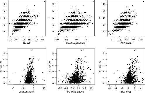
Figure 1: Comparison of SEE with other estimators of CMS and CVS for the abalone data. In the upper panels, the x-axes are the predictors obtained by RMAVE, Zhu–Dong–Li and SEE  estimates for the CMS; the y-axes are the abalones’ ages. In the lower panels, the x-axes are the predictors derived from Zhu–Zhu, Zhu–Dong–Li and SEE estimates of the CVS; the y-axes are the estimated absolute residuals.

To give an objective numerical comparison, we use a bootstrapped error measurement akin to that introduced by Ye and Weiss (2003), which is reasonable because all estimators involved are consistent. Since the predictors in the abalone data set are highly correlated, two estimates of $\beta$ that span substantially different linear spaces can correspond to nearly identical $\beta^{\mathsf{T}}X$. For this reason, rather than measuring the error in $\hat{\beta}$, as we did in the simulations, here we directly measure the error in $\hat{\beta}^{\mathsf{T}}X$. Specifically, we generate $500$ bootstrap samples, and for each sample we compute the estimate $\tilde{\beta}$. We also compute the full-sample estimate $\hat{\beta}$. For each bootstrap sample, we evaluate the sample correlation between

$$\bigl{\{}\tilde{\beta}^{\mathsf{T}}X_{1},\ldots,\tilde{\beta}^{\mathsf{T}}X_{n}\bigr{\}},\qquad\bigl{\{}\hat{\beta}^{\mathsf{T}}X_{1},\ldots,\hat{\beta}^{\mathsf{T}}X_{n}\bigr{\}}.$$

We denote sample correlations for the 500 bootstrap samples as $\rho_{1},\ldots,\rho_{500}$. We then compute $1-\sum_{i=1}^{500}|\rho_{i}|/500$ and call it the bootstrap error of the estimator. The result is summarized in the Table 5.

Table 5: Bootstrap error of the estimators

Functionals	Estimators
$E(Y|X)$	RMAVE	Zhu–Dong–Li	SEE
	$0.145$	$0.009$	$0.003$
$\operatorname{Var}(Y|X)$	Zhu–Zhu	Zhu–Dong–Li	SEE
	$0.213$	$0.131$	$0.105$

We see that SEE is the top performer for estimating both CMS and CVS, followed by the estimator of Zhu, Dong and Li (2013), and then by RMAVE. We also observe that the estimation of central variance subspace is in general less accurate than that of central mean subspace, as has been observed in many other cases, for example, in Zhu, Dong and Li (2013).

12 Discussions

In this paper, we introduce a general paradigm for sufficient dimension reduction with respect to a conditional statistical functional, along with semiparametrically efficient procedures to estimate the sufficient predictors of that functional. This method is particularly useful when we want to select sufficient predictors with some specific purposes in mind, such as estimating the conditional quantiles in a population. This work is a continuation, synthesis and refinement of previous works on nonparametric mean regression, nonparametric quantile regression and nonparametric estimation of heteroscedasticity, under the unifying framework of SDR. It provides us with tools to explore the detailed structures of the central subspace, making SDR more specific to our goals. Our work has also substantially broadened the scope of the semiparametric approach recently introduced to SDR by Ma and Zhu (2012, 2013a and 2013b).

In a wide range of simulation studies, the SEE is shown to outperform several previously proposed estimators for conditional mean, conditional quantile and conditional variance. Moreover, the theoretical semiparametric lower bound is approximately achieved by the actual error based on simulation. Finally, the algorithm we developed for SEE has a special advantage over that proposed in Ma and Zhu (2013a): it does not rely on any specific parameterization of the central subspace, which means we do not need to subjectively assign any element of $\beta$ to be nonzero from the outset.

References

- Bickel et al. (1993) {bbook}[mr] \bauthor\bsnmBickel, \bfnmPeter J.\binitsP. J., \bauthor\bsnmKlaassen, \bfnmChris A. J.\binitsC. A. J., \bauthor\bsnmRitov, \bfnmYa’acov\binitsY. and \bauthor\bsnmWellner, \bfnmJon A.\binitsJ. A. (\byear1993). \btitleEfficient and Adaptive Estimation for Semiparametric Models. \bpublisherJohns Hopkins Univ. Press, \blocationBaltimore, MD. \bidmr=1245941 \bptokimsref\endbibitem
- Cook (1994) {bincollection}[auto:STB—2014/01/06—10:16:28] \bauthor\bsnmCook, \bfnmR. D.\binitsR. D. (\byear1994). \btitleUsing dimension-reduction subspaces to identify important inputs in models of physical systems. In \bbooktitle1994 Proceedings of the Section on Physical and Engineering Sciences \bpages18–25. \bpublisherAmerican Statistical Association, \blocationAlexandria, VA. \bptokimsref\endbibitem
- Cook (1996) {barticle}[mr] \bauthor\bsnmCook, \bfnmR. Dennis\binitsR. D. (\byear1996). \btitleGraphics for regressions with a binary response. \bjournalJ. Amer. Statist. Assoc. \bvolume91 \bpages983–992. \biddoi=10.2307/2291717, issn=0162-1459, mr=1424601 \bptokimsref\endbibitem
- Cook (1998) {bbook}[mr] \bauthor\bsnmCook, \bfnmR. Dennis\binitsR. D. (\byear1998). \btitleRegression Graphics: Ideas for Studying Regressions Through Graphics. \bpublisherWiley, \blocationNew York. \biddoi=10.1002/9780470316931, mr=1645673 \bptokimsref\endbibitem
- Cook and Li (2002) {barticle}[mr] \bauthor\bsnmCook, \bfnmR. Dennis\binitsR. D. and \bauthor\bsnmLi, \bfnmBing\binitsB. (\byear2002). \btitleDimension reduction for conditional mean in regression. \bjournalAnn. Statist. \bvolume30 \bpages455–474. \biddoi=10.1214/aos/1021379861, issn=0090-5364, mr=1902895 \bptokimsref\endbibitem
- Cook and Weisberg (1991) {barticle}[auto] \bauthor\bsnmCook, \bfnmR. D.\binitsR. D. and \bauthor\bsnmWeisberg, \bfnmS.\binitsS. (\byear1991). \btitleDiscussion of “Sliced inverse regression for dimension reduction.” \bjournalJ. Amer. Statist. Assoc. \bvolume86 \bpages316–342. \bptokimsref\endbibitem
- Dong and Li (2010) {barticle}[mr] \bauthor\bsnmDong, \bfnmYuexiao\binitsY. and \bauthor\bsnmLi, \bfnmBing\binitsB. (\byear2010). \btitleDimension reduction for non-elliptically distributed predictors: Second-order methods. \bjournalBiometrika \bvolume97 \bpages279–294. \biddoi=10.1093/biomet/asq016, issn=0006-3444, mr=2650738 \bptokimsref\endbibitem
- Edelman, Arias and Smith (1999) {barticle}[mr] \bauthor\bsnmEdelman, \bfnmAlan\binitsA., \bauthor\bsnmArias, \bfnmTomás A.\binitsT. A. and \bauthor\bsnmSmith, \bfnmSteven T.\binitsS. T. (\byear1999). \btitleThe geometry of algorithms with orthogonality constraints. \bjournalSIAM J. Matrix Anal. Appl. \bvolume20 \bpages303–353. \biddoi=10.1137/S0895479895290954, issn=0895-4798, mr=1646856 \bptnotecheck year \bptokimsref\endbibitem
- Godambe (1960) {barticle}[mr] \bauthor\bsnmGodambe, \bfnmV. P.\binitsV. P. (\byear1960). \btitleAn optimum property of regular maximum likelihood estimation. \bjournalAnn. Math. Statist. \bvolume31 \bpages1208–1211. \bidissn=0003-4851, mr=0123385 \bptokimsref\endbibitem
- Härdle, Hall and Ichimura (1993) {barticle}[mr] \bauthor\bsnmHärdle, \bfnmWolfgang\binitsW., \bauthor\bsnmHall, \bfnmPeter\binitsP. and \bauthor\bsnmIchimura, \bfnmHidehiko\binitsH. (\byear1993). \btitleOptimal smoothing in single-index models. \bjournalAnn. Statist. \bvolume21 \bpages157–178. \biddoi=10.1214/aos/1176349020, issn=0090-5364, mr=1212171 \bptokimsref\endbibitem
- Kong and Xia (2012) {barticle}[mr] \bauthor\bsnmKong, \bfnmEfang\binitsE. and \bauthor\bsnmXia, \bfnmYingcun\binitsY. (\byear2012). \btitleA single-index quantile regression model and its estimation. \bjournalEconometric Theory \bvolume28 \bpages730–768. \biddoi=10.1017/S0266466611000788, issn=0266-4666, mr=2959124 \bptokimsref\endbibitem
- Li (1991) {barticle}[mr] \bauthor\bsnmLi, \bfnmKer-Chau\binitsK.-C. (\byear1991). \btitleSliced inverse regression for dimension reduction. \bjournalJ. Amer. Statist. Assoc. \bvolume86 \bpages316–342. \bidissn=0162-1459, mr=1137117 \bptokimsref\endbibitem
- Li (1992) {barticle}[mr] \bauthor\bsnmLi, \bfnmKer-Chau\binitsK.-C. (\byear1992). \btitleOn principal Hessian directions for data visualization and dimension reduction: Another application of Stein’s lemma. \bjournalJ. Amer. Statist. Assoc. \bvolume87 \bpages1025–1039. \bidissn=0162-1459, mr=1209564 \bptokimsref\endbibitem
- Li, Artemiou and Li (2011) {barticle}[mr] \bauthor\bsnmLi, \bfnmBing\binitsB., \bauthor\bsnmArtemiou, \bfnmAndreas\binitsA. and \bauthor\bsnmLi, \bfnmLexin\binitsL. (\byear2011). \btitlePrincipal support vector machines for linear and nonlinear sufficient dimension reduction. \bjournalAnn. Statist. \bvolume39 \bpages3182–3210. \biddoi=10.1214/11-AOS932, issn=0090-5364, mr=3012405 \bptokimsref\endbibitem
- Li and Dong (2009) {barticle}[mr] \bauthor\bsnmLi, \bfnmBing\binitsB. and \bauthor\bsnmDong, \bfnmYuexiao\binitsY. (\byear2009). \btitleDimension reduction for nonelliptically distributed predictors. \bjournalAnn. Statist. \bvolume37 \bpages1272–1298. \biddoi=10.1214/08-AOS598, issn=0090-5364, mr=2509074 \bptokimsref\endbibitem
- Li, Li and Zhu (2010) {barticle}[mr] \bauthor\bsnmLi, \bfnmLexin\binitsL., \bauthor\bsnmLi, \bfnmBing\binitsB. and \bauthor\bsnmZhu, \bfnmLi-Xing\binitsL.-X. (\byear2010). \btitleGroupwise dimension reduction. \bjournalJ. Amer. Statist. Assoc. \bvolume105 \bpages1188–1201. \biddoi=10.1198/jasa.2010.tm09643, issn=0162-1459, mr=2752614 \bptokimsref\endbibitem
- Li and McCullagh (1994) {barticle}[mr] \bauthor\bsnmLi, \bfnmBing\binitsB. and \bauthor\bsnmMcCullagh, \bfnmPeter\binitsP. (\byear1994). \btitlePotential functions and conservative estimating functions. \bjournalAnn. Statist. \bvolume22 \bpages340–356. \biddoi=10.1214/aos/1176325372, issn=0090-5364, mr=1272087 \bptokimsref\endbibitem
- Li, Zha and Chiaromonte (2005) {barticle}[mr] \bauthor\bsnmLi, \bfnmBing\binitsB., \bauthor\bsnmZha, \bfnmHongyuan\binitsH. and \bauthor\bsnmChiaromonte, \bfnmFrancesca\binitsF. (\byear2005). \btitleContour regression: A general approach to dimension reduction. \bjournalAnn. Statist. \bvolume33 \bpages1580–1616. \biddoi=10.1214/009053605000000192, issn=0090-5364, mr=2166556 \bptokimsref\endbibitem
- Luo, Li and Yin (2014) {bmisc}[auto] \bauthor\bsnmLuo, \bfnmW.\binitsW., \bauthor\bsnmLi, \bfnmB.\binitsB. and \bauthor\bsnmYin, \bfnmX.\binitsX. (\byear2014). \bhowpublishedSupplement to “On efficient dimension reduction with respect to a statistical functional of interest.” DOI:\doiurl10.1214/13-AOS1195SUPP. \bptokimsref\endbibitem
- Ma and Zhu (2012) {barticle}[mr] \bauthor\bsnmMa, \bfnmYanyuan\binitsY. and \bauthor\bsnmZhu, \bfnmLiping\binitsL. (\byear2012). \btitleA semiparametric approach to dimension reduction. \bjournalJ. Amer. Statist. Assoc. \bvolume107 \bpages168–179. \biddoi=10.1080/01621459.2011.646925, issn=0162-1459, mr=2949349 \bptokimsref\endbibitem
- Ma and Zhu (2013a) {barticle}[mr] \bauthor\bsnmMa, \bfnmYanyuan\binitsY. and \bauthor\bsnmZhu, \bfnmLiping\binitsL. (\byear2013a). \btitleEfficient estimation in sufficient dimension reduction. \bjournalAnn. Statist. \bvolume41 \bpages250–268. \biddoi=10.1214/12-AOS1072, issn=0090-5364, mr=3059417 \bptokimsref\endbibitem
- Ma and Zhu (2013b) {barticle}[mr] \bauthor\bsnmMa, \bfnmYanyuan\binitsY. and \bauthor\bsnmZhu, \bfnmLiping\binitsL. (\byear2013b). \btitleEfficiency loss and the linearity condition in dimension reduction. \bjournalBiometrika \bvolume100 \bpages371–383. \biddoi=10.1093/biomet/ass075, issn=0006-3444, mr=3068440 \bptokimsref\endbibitem
- McCullagh (1987) {bbook}[mr] \bauthor\bsnmMcCullagh, \bfnmPeter\binitsP. (\byear1987). \btitleTensor Methods in Statistics. \bpublisherChapman & Hall, \blocationLondon. \bidmr=0907286 \bptokimsref\endbibitem
- Székely and Rizzo (2009) {barticle}[mr] \bauthor\bsnmSzékely, \bfnmGábor J.\binitsG. J. and \bauthor\bsnmRizzo, \bfnmMaria L.\binitsM. L. (\byear2009). \btitleBrownian distance covariance. \bjournalAnn. Appl. Stat. \bvolume3 \bpages1236–1265. \biddoi=10.1214/09-AOAS312, issn=1932-6157, mr=2752127 \bptokimsref\endbibitem
- van der Vaart (1998) {bbook}[mr] \bauthor\bsnmvan der Vaart, \bfnmA. W.\binitsA. W. (\byear1998). \btitleAsymptotic Statistics. \bseriesCambridge Series in Statistical and Probabilistic Mathematics \bvolume3. \bpublisherCambridge Univ. Press, \blocationCambridge. \bidmr=1652247 \bptokimsref\endbibitem
- Wang and Xia (2008) {barticle}[mr] \bauthor\bsnmWang, \bfnmHansheng\binitsH. and \bauthor\bsnmXia, \bfnmYingcun\binitsY. (\byear2008). \btitleSliced regression for dimension reduction. \bjournalJ. Amer. Statist. Assoc. \bvolume103 \bpages811–821. \biddoi=10.1198/016214508000000418, issn=0162-1459, mr=2524332 \bptokimsref\endbibitem
- Xia (2007) {barticle}[mr] \bauthor\bsnmXia, \bfnmYingcun\binitsY. (\byear2007). \btitleA constructive approach to the estimation of dimension reduction directions. \bjournalAnn. Statist. \bvolume35 \bpages2654–2690. \biddoi=10.1214/009053607000000352, issn=0090-5364, mr=2382662 \bptokimsref\endbibitem
- Xia, Tong and Li (2002) {barticle}[mr] \bauthor\bsnmXia, \bfnmYingcun\binitsY., \bauthor\bsnmTong, \bfnmHowell\binitsH. and \bauthor\bsnmLi, \bfnmW. K.\binitsW. K. (\byear2002). \btitleSingle-index volatility models and estimation. \bjournalStatist. Sinica \bvolume12 \bpages785–799. \bidissn=1017-0405, mr=1929964 \bptokimsref\endbibitem
- Xia et al. (2002) {barticle}[mr] \bauthor\bsnmXia, \bfnmYingcun\binitsY., \bauthor\bsnmTong, \bfnmHowell\binitsH., \bauthor\bsnmLi, \bfnmW. K.\binitsW. K. and \bauthor\bsnmZhu, \bfnmLi-Xing\binitsL.-X. (\byear2002). \btitleAn adaptive estimation of dimension reduction space. \bjournalJ. R. Stat. Soc. Ser. B Stat. Methodol. \bvolume64 \bpages363–410. \biddoi=10.1111/1467-9868.03411, issn=1369-7412, mr=1924297 \bptnotecheck related \bptokimsref\endbibitem
- Ye and Weiss (2003) {barticle}[mr] \bauthor\bsnmYe, \bfnmZhishen\binitsZ. and \bauthor\bsnmWeiss, \bfnmRobert E.\binitsR. E. (\byear2003). \btitleUsing the bootstrap to select one of a new class of dimension reduction methods. \bjournalJ. Amer. Statist. Assoc. \bvolume98 \bpages968–979. \biddoi=10.1198/016214503000000927, issn=0162-1459, mr=2041485 \bptokimsref\endbibitem
- Yin and Cook (2002) {barticle}[mr] \bauthor\bsnmYin, \bfnmXiangrong\binitsX. and \bauthor\bsnmCook, \bfnmR. Dennis\binitsR. D. (\byear2002). \btitleDimension reduction for the conditional th moment in regression. \bjournalJ. R. Stat. Soc. Ser. B Stat. Methodol. \bvolume64 \bpages159–175. \biddoi=10.1111/1467-9868.00330, issn=1369-7412, mr=1904698 \bptokimsref\endbibitem
- Yin and Li (2011) {barticle}[mr] \bauthor\bsnmYin, \bfnmXiangrong\binitsX. and \bauthor\bsnmLi, \bfnmBing\binitsB. (\byear2011). \btitleSufficient dimension reduction based on an ensemble of minimum average variance estimators. \bjournalAnn. Statist. \bvolume39 \bpages3392–3416. \biddoi=10.1214/11-AOS950, issn=0090-5364, mr=3012413 \bptokimsref\endbibitem
- Yin, Li and Cook (2008) {barticle}[mr] \bauthor\bsnmYin, \bfnmXiangrong\binitsX., \bauthor\bsnmLi, \bfnmBing\binitsB. and \bauthor\bsnmCook, \bfnmR. Dennis\binitsR. D. (\byear2008). \btitleSuccessive direction extraction for estimating the central subspace in a multiple-index regression. \bjournalJ. Multivariate Anal. \bvolume99 \bpages1733–1757. \biddoi=10.1016/j.jmva.2008.01.006, issn=0047-259X, mr=2444817 \bptokimsref\endbibitem
- Zhu, Dong and Li (2013) {barticle}[mr] \bauthor\bsnmZhu, \bfnmLiping\binitsL., \bauthor\bsnmDong, \bfnmYuexiao\binitsY. and \bauthor\bsnmLi, \bfnmRunze\binitsR. (\byear2013). \btitleSemiparametric estimation of conditional heteroscedasticity via single-index modeling. \bjournalStatist. Sinica \bvolume23 \bpages1235–1255. \bidissn=1017-0405, mr=3114712 \bptnotecheck year \bptokimsref\endbibitem
- Zhu and Zeng (2006) {barticle}[mr] \bauthor\bsnmZhu, \bfnmYu\binitsY. and \bauthor\bsnmZeng, \bfnmPeng\binitsP. (\byear2006). \btitleFourier methods for estimating the central subspace and the central mean subspace in regression. \bjournalJ. Amer. Statist. Assoc. \bvolume101 \bpages1638–1651. \biddoi=10.1198/016214506000000140, issn=0162-1459, mr=2279485 \bptokimsref\endbibitem
- Zhu and Zhu (2009) {barticle}[mr] \bauthor\bsnmZhu, \bfnmLi-Ping\binitsL.-P. and \bauthor\bsnmZhu, \bfnmLi-Xing\binitsL.-X. (\byear2009). \btitleDimension reduction for conditional variance in regressions. \bjournalStatist. Sinica \bvolume19 \bpages869–883. \bidissn=1017-0405, mr=2514192 \bptokimsref\endbibitem
- Zou and Yuan (2008) {barticle}[mr] \bauthor\bsnmZou, \bfnmHui\binitsH. and \bauthor\bsnmYuan, \bfnmMing\binitsM. (\byear2008). \btitleComposite quantile regression and the oracle model selection theory. \bjournalAnn. Statist. \bvolume36 \bpages1108–1126. \biddoi=10.1214/07-AOS507, issn=0090-5364, mr=2418651 \bptokimsref\endbibitem