SLAC-PUB-15917
Fun with New Gauge Bosons at 100 TeV
Abstract
The production of new gauge bosons is a standard benchmark for the exploration of the physics capabilities of future colliders. The TeV Future Hadron Collider will make a major step in our ability to search for and explore the properties of such new states. In this paper, employing traditional models to make contact with the past and more recent literature, we not only establish in detail the discovery and exclusion reaches for both the and within these models but, more importantly, we also examine the capability of the FHC to extract information relevant for the determination of the couplings of the to the fermions of the Standard Model as well as the helicity of the corresponding couplings. This is a necessary first step in determining the nature of the underlying theory which gave rise to these states.
1 Introduction and Background
Interest is growing in the physics of a possible Future Hadron Collider (FHC) which will take over the Energy Frontier sometime after the running of the HL-LHC been has completed[1]. CERN has already begun a 5-year study to investigate this possibility[2]. Presently, the FHC is currently envisioned as having a center-of-mass energy of TeV and having the capability to accumulate integrated luminosities of order ab-1 or greater222Interestingly, this energy represents as large of a step above that of the LHC as the LHC was above the Tevatron.. As is well-known, the LHC has/had ‘the origin of electroweak symmetry breaking in the Standard Model’ as a known ’no-loose’ physics target to set its energy scale. Clearly, with the discovery of the Higgs boson in 2012, the LHC has already been quite successful in this regard. The 100 TeV energy for the FHC, on the otherhand, represents an educated extrapolation of what might be possible given foreseeable technological improvements without incurring ‘prohibitive’ costs while simultaneously allowing for the opening up of potential new physics thresholds. The FHC is thus truly a machine of exploration as were the accelerators of earlier generations. Of course, in a more general context, the physics associated with such higher energy hadron colliders beyond the LHC has been frequently discussed from time to time over the past two decades[3] since the cancellation of the SSC.
One of the historic and standard new physics benchmarks that is always employed in the study of the potential capabilities of future colliders is the production and examination of new neutral () and charged () gauge bosons[4] the reason being that they are a relatively common occurrence in many beyond the Standard Model (BSM) scenarios and they (usually) have relatively clean leptonic signatures. This may be of particular relevance at a high luminosity TeV machine where one can presently only guess at the difficulty of making measurements within this challenging hadronic environment. While previous works[5] have provided us with some idea as to what to expect as far as the discovery potential for might be at the FHC, here we wish to go somewhat further in both the quantification of these results and to address the question of how well such new states might be studied assuming that they are indeed discovered. In order to make direct contact with many past studies[4, 5, 6] we will restrict ourselves to the somewhat traditional set of BSM models containing considered there. We remind the reader that this does not in any way exhaust the range of possibilities for such new states but it does give us a respectable range of predictions to examine for what one might expect at 100 TeV. Here we will also restrict our attention to the relatively safe final states which employ at least one (very) high lepton trigger due to the unknown nature of the hadronic environment and pile-up conditions the detectors may have to deal with at 100 TeV as mentioned earlier. Furthermore, we will concentrate mostly on electron final states as muon resolution for (many) mult-TeV muons is likely to be difficult with the typical magnetic fields that are currently available given finite detector size even when we allow for factors of two scaling in both these quantities. We note that if the muon pair mass resolution is sufficiently degraded this will have a significant impact on narrow searches in this channel.
Present measurements by both ATLAS[7, 8] and CMS[9, 10] at TeV with fb-1 of integrated luminosity can only provide lower bounds on the masses of possible new states. For example, if these states have couplings identical to those of the corresponding SM gauge bosons (i.e., the so-called SSM ‘model’) their masses must exceed 2.96 and 3.35 TeV, respectively. Of course for other types of couplings, quite different, generally somewhat weaker results are obtained as in the case of an -inspired [11]. Eventually, at the 14 TeV HL-LHC, search sensitivities for the same and states may be as large as TeV[12] depending upon whether they are discovered or excluded. In what follows we will generally assume that the masses of these new states are beyond the reach of the HL-LHC at least to study in any detail even if they were to be in fact discovered there.
In the analysis below we will examine not only the discovery and exclusion rates for these new states at 100 TeV but also survey how data obtainable by experiments at the FHC may be used to determine their detailed properties through a number of different observables. This survey is not meant to be either exhaustive or conclusive but only to provide a first glimpse at what some of these possibilities might be based on earlier studies performed for other hadron colliders333We will not consider the interesting possibility to study this new physics with polarized proton beams here[13].. Much work will still be needed to examine the feasibility of the use of the many observables discussed below for the study of new gauge bosons at the FHC. We first consider new gauge bosons in the next Section and then turn our attention to the case in Section 3. Section 4 contains a discussion and our conclusions. The Appendix considers the case of SSM and gauge bosons but with non-SSM coupling strengths.
2 New Bosons
The first issue we address is the obvious one: what is the mass reach for gauge boson discovery or exclusion at TeV? The usual approach as performed at the LHC has two components: () compare the expected opposite-sign dilepton invariant mass distribution with the SM expectations and look for excesses at high mass and then either claim an excess or set a limit () compare the expected number of (excess?) dilepton events with the the narrow-width approximation (NWA) cross section (times leptonic branching fraction) for the the within a given BSM model. To perform the corresponding calculations here for the FHC we will assume a detector below with a lepton rapidity coverage () and electron EM energy resolution similar to that of the present ATLAS detector and, to be specific, we will make use of the default NLO CTEQ6.6 pdfs[14] and scale the relevant cross sections employing NLO K-factors[15] when obtaining our numerical results444We remind the reader that there are presently significant uncertainties in extrapolating the currently available pdfs up to 100 TeV. We note that employing the NNLO CT10 pdfs gives the same cross section results as used here up to corrections of order percent.. (and correspondingly below) partial widths will be calculated including NLO and partial NNLO QCD corrections as well as the corresponding NLO QED corrections. As a final comment, we note that these calculations will be performed using a fixed-width prescription for the but one can easily check that identical results are obtained using the running-width instead given the resulting level of statistics.
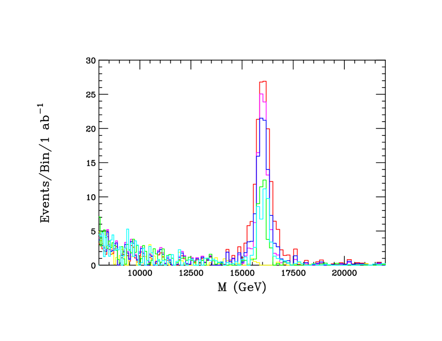
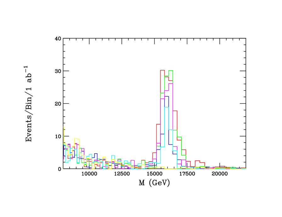
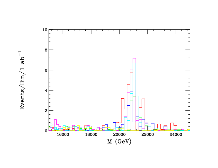
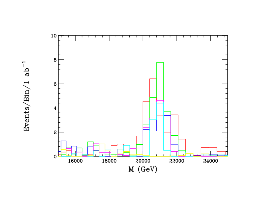
To begin our analysis it is instructive to examine the resonance signal structure for production in the Drell-Yan dielectron mass distribution at 100 TeV. A first example of this is shown in Figs. 1 and 2 which show the Drell-Yan mass distributions for several different models assuming a mass of either 16 or 21 TeV along with the associated SM backgrounds taking an integrated luminosity of 1 ab-1.555In what follows we will always assume that any new gauge bosons are un-mixed with their SM counterparts and that they decay only into the known SM states in obtaining all numerical results. From the upper panel of Fig, 1, it is fairly obvious that for a mass of 16 TeV with this luminosity all of these models predict an easily visible signal above the SM background. In the lower panel we see how the signals will respond if the dilepton mass resolution were to become worse by a factor of 2; clearly all the states still remain easily visible. It is important to note that in most of these models the width to mass ratio of the is quite comparable to and frequently less than these resolutions which imply that it is the resolution itself that often controls the ‘lineshape’ and not the actual width. On the otherhand, when the mass is increased to 21 TeV (not a randomly chosen number), as seen in Fig. 2, it is a bit less obvious how statistically convincing the signal remains in all these different cases. However, by counting events, we find that most of these models would likely be discovered although several lie (very) close to the statistical boundary signal events in this mass region since it essentially background-free. Of course, the corresponding dimuon sample could also be potentially helpful here but given the likely inferior mass resolution for dimuons its not clear by how much without some further assumptions. Certainly the dimuon distribution would also likely show a high mass excess confirming that in dielectrons but would not yield a very reliable determination of the peak mass value since this excess would likely be quite broadly distributed. It would seem that for this class of models TeV represents a rough estimate of the rough lower mass limit for discovery.
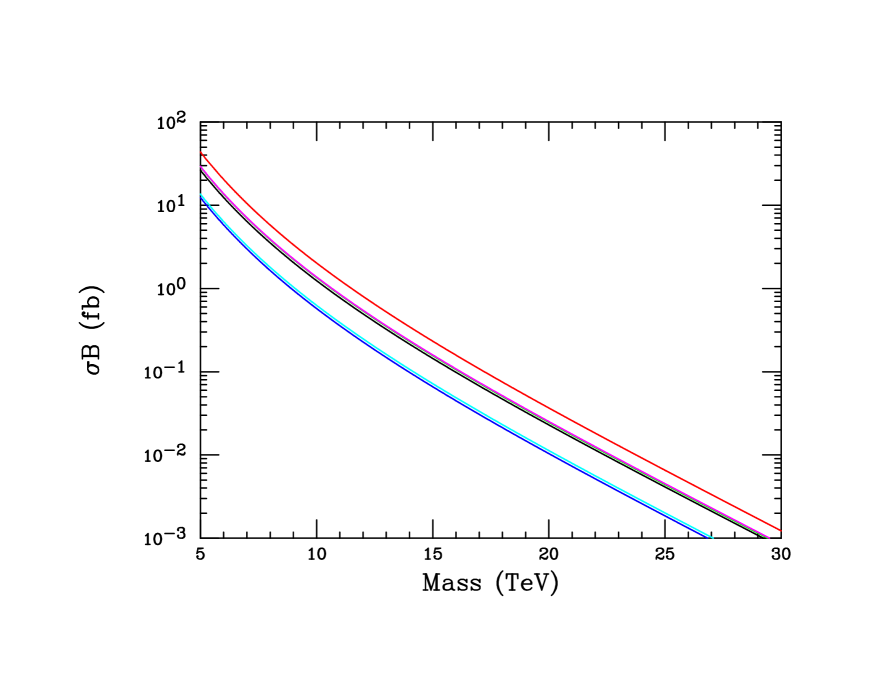
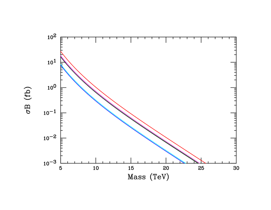
These results on both potential discovery and possible exclusion can be further summarized by the content of Fig. 3 and in Table 1. Fig. 3 shows the dilepton production signal cross section via the arising in different models calculated in the NWA including acceptance cuts for both and 100 TeV. In this Figure we see several things: for example, even within this rather restricted set of models the cross sections can vary by about a factor of at any given mass value. Furthermore, we see that at large masses, for a fixed value of the cross section, going from to 100 TeV will allow us to increase the reach by roughly TeV. For later discussions, Table 1 shows the actual numerical values of these cross sections for masses of 10, 15 and 20 TeV and also the expected discovery and exclusion reaches in TeV (assuming an integrated luminosity of 1 ab-1) for the same set of models. These values will be important when we examine statistical errors on the various quantities we introduce below. We also note here that an increase in the integrated luminosity by a factor of 3(10) will increase both the discovery and exclusion reaches by roughly TeV for all these models.
| Model | 10 TeV | 15 TeV | 20 TeV | Disc. | Excl. |
|---|---|---|---|---|---|
| SSM | 2021. | 232.6 | 36.65 | 23.8 | 27.3 |
| LRM | 1353. | 156.1 | 24.62 | 22.6 | 26.1 |
| 573.7 | 65.93 | 10.37 | 20.1 | 23.6 | |
| 1372. | 159.0 | 25.18 | 22.7 | 26.2 | |
| 626.8 | 71.82 | 11.38 | 20.3 | 23.8 | |
| I | 1241. | 144.4 | 22.94 | 22.4 | 25.7 |
Once a has been discovered, we want to learn which model, if any, it corresponds to which means that we need to learn about its couplings to the various SM fields. If these couplings are generation independent (which would appear likely given current flavor physics constraints) this will involve 7 independent parameters. Furthermore, if the new gauge group to which the belongs commutes with the SM group factor, which is true for GUT groups such as the LRM and , there remain only 5 such parameters corresponding to the couplings of the to , , and 666Of course the SSM does not fall in this class as it is merely used as a benchmark so that there are still 7 distinct couplings in this case as for the SM (by definition).. Note that within these GUT-like frameworks any gauge anomalies that may apparently exist are canceled by the presence of additional fermions which are either SM singlets or are vector-like with respect to the SM interactions. As noted above, when making the numerical calculations that we will present below it will always be assumed that all such fields are kinematically inaccessible in the decays of the new gauge bosons that we consider. However, since such states might participate in decays, using observables that are sensitive to the existence of these states in order to identify the or themselves is problematic and may lead to the wrong conclusions[4]. Interestingly, we note that reducing the leptonic branching fraction by a factor of two due to new open channels will result in a reduction of the discovery and exclusion reaches by roughly TeV in all cases.
It should be noted here for completeness that the observation of a new high mass resonance in the opposite-sign dilepton channel does not necessarily imply that a has been discovered. For example, we have not discussed here the importance of the determination of the resonance’s spin via the leptonic angular distribution [4]. One could imagine that such a resonance could be spin-2 (e.g., a Kaluza-Klein graviton) or even spin-0 (e.g., an R-Parity violating sneutrino) so the discovery of a spin-1 state is assumed in the discussion that follows.
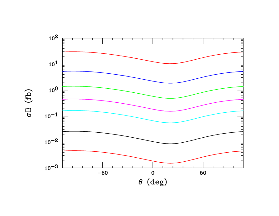
Clearly the production cross section times leptonic branching fraction of the itself is a potentially interesting observable for determining fermionic couplings. As we saw in Table 1 above, these cross sections vary substantially from model to model, even within the scenario itself as is shown in Fig. 4 where a variation of more than a factor of 3 is observed. Trivially, this observable on its own is obviously sensitive to variations in the different coupling parameters. However, the value of the leptonic branching fraction employed to obtain these results assumes that the can decay to only SM particles. Thus, strictly speaking, we cannot use this observable (alone) to obtain determinations of the couplings. Of course, as has long been known, ratios of such cross section times branching fractions are insensitive to any additional decay modes that the may have and we will make use of this result below.
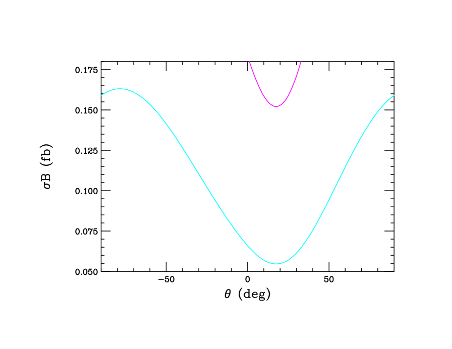
With this issue in mind and using the same production channel (dileptons) as for discovery there are other observables that one can use to obtain coupling information that are insensitive to any potential additional decay models. The most obvious one is obtained by just rescaling the overall signal rate by the extracted width of the resonance. In the NWA we see this quantity is just the product which is clearly independent of whether or not additional decay modes are present (since the product is just the leptonic width of the ) and this remains true to a good approximation even when a more detailed calculation is performed. Results for this quantity using the NWA can be seen in Table 2 and in Fig. 5. This Figure shows the NWA evaluation of this quantity in the case demonstrating its respectable coupling sensitivity, varying by a factor of just within this model framework while the Table shows variations as large as a factor of . To use this quantity we need to extract not only the production cross section in the leptonic channel but also we need to determine the width by a de-convolution of the mass resolution in the peak region. An early ATLAS study of this quantity for the 14 TeV LHC[17] for 10 fb-1 of simulated data suggests that this may be possible with slightly larger than statistical errors, e.g., . Clearly further study of this quantity at higher energies and masses would be valuable.
| Model | 10 TeV | 15 TeV | 20 TeV |
|---|---|---|---|
| SSM | 0.6108 | 0.1054 | 0.0221 |
| LRM | 0.2815 | 0.0487 | 0.0102 |
| 0.0308 | 0.0053 | 0.0011 | |
| 0.1615 | 0.0281 | 0.0059 | |
| 0.0404 | 0.0069 | 0.0015 | |
| I | 0.1326 | 0.0231 | 0.0049 |
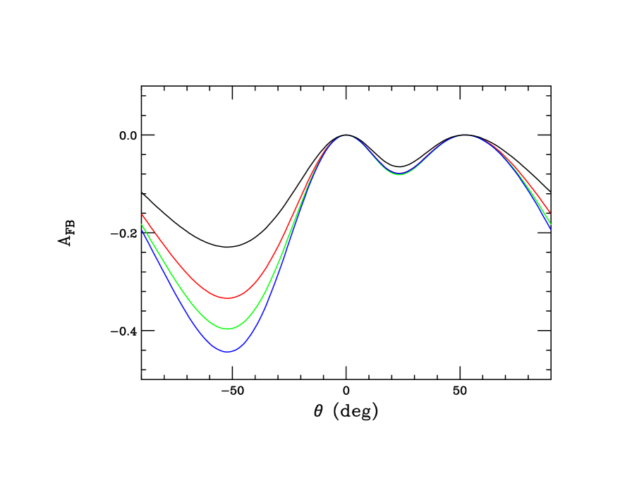
Perhaps the most well known example of a coupling-sensitive observable that makes use of the dilepton discovery channel is which can be obtained in principle from the lepton’s angular distribution. In the rest frame, with being defined between the initial quark, , and outgoing direction this distribution is given by . Fig. 6 shows two very idealized examples for these distributions (before any acceptance corrections, etc) assuming 300 dilepton events are observed. These figures demonstrate the typical level of statistics required to determine with some reliability (given the typical asymmetries predicted in many models) in an idealized situation. To get closer to reality two additional requirements are obvious: () an acceptance correction needs to be applied to account for the cut of on the lepton rapidity. This effectively reduces the the number of events at large values of thus reducing the overall sensitivity to any non-zero asymmetry. Even more importantly, () a correction must be applied to identify which direction along the collision axis is to be identified with that of the initial . A first approximation for this (that can be later more fully performed by Monte Carlo) is to note that, most of the time, due to the pdfs, the direction can be identified with boost direction of the which can be easily reconstructed. This requires a minimum cut on , here chosen to be for numerical purposes, which, at the very least will further reduce the level of statistics. This cut becomes quite significant as the mass increases and the rapidity becomes ever more central with the maximum boost being for masses of 10(15, 20) TeV at TeV.
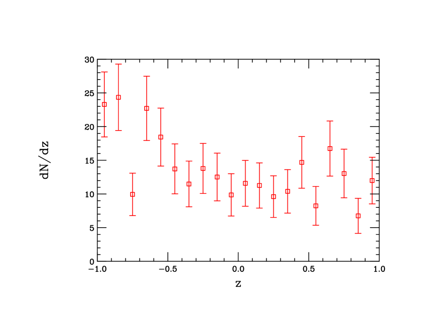
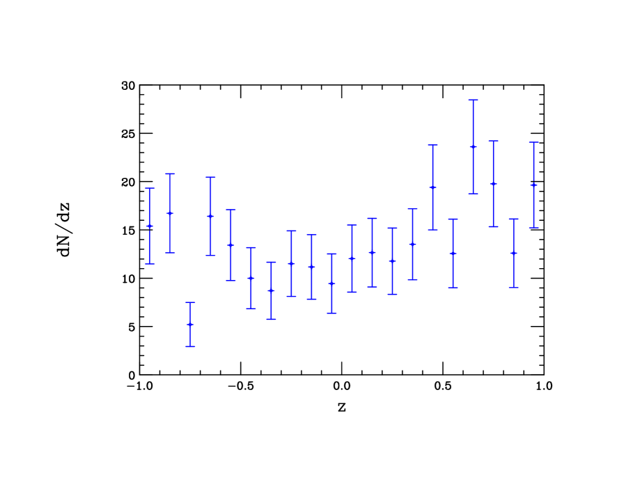
This discussion informs us that a reasonable level of statistics, roughly on the order of signal events, will be required for a respectable determination of . Such event rates are achievable for masses roughly TeV below the mass where discovery is possible. This implies, e.g., that for an SSM a reliable value of is not obtainable if the mass is in excess of 18 TeV or so unless luminosities in excess of the canonical 1 ab-1 value that we have assumed here are achievable.
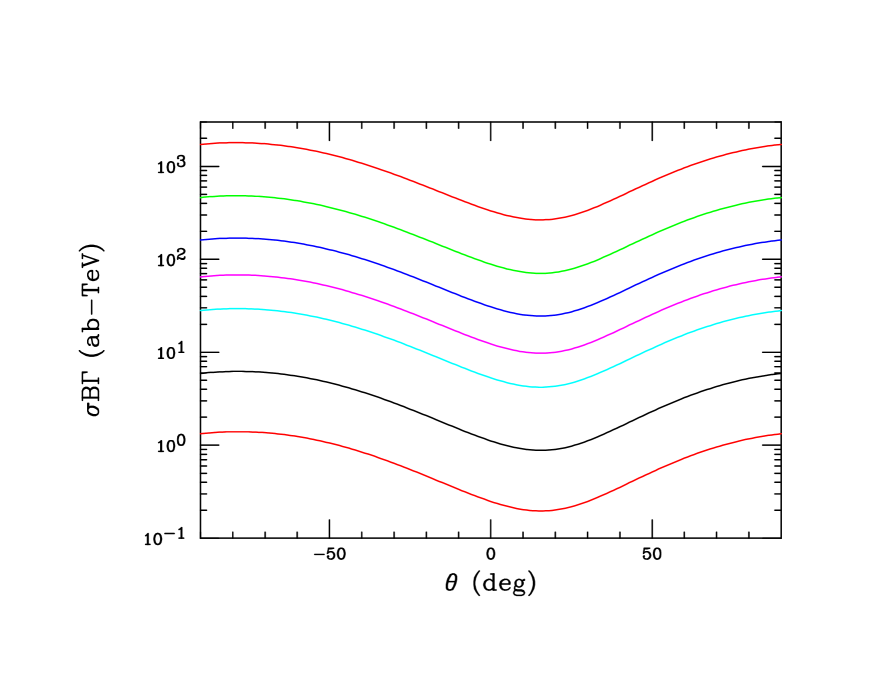
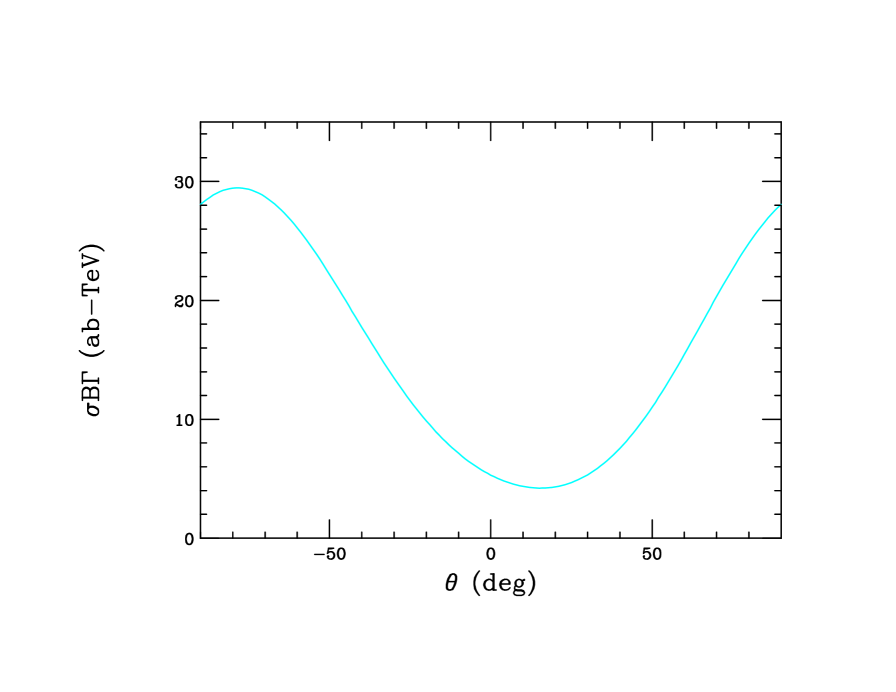
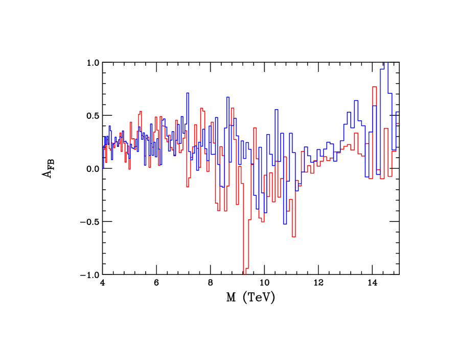
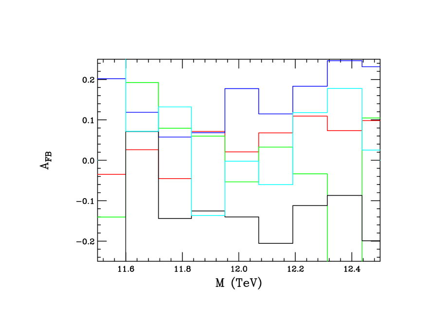
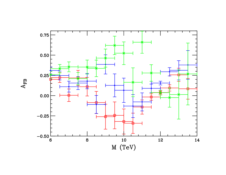
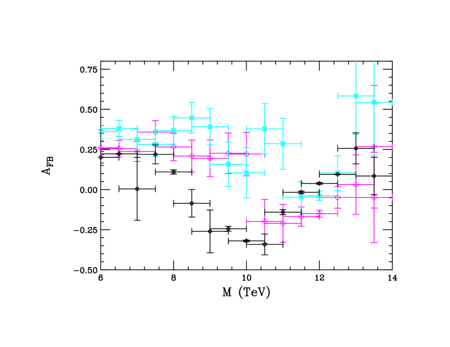
Of course, if is indeed measurable with some precision it will provide the SM fermion coupling sensitivity as advertised as can be seen in the upper panel of Fig 7 and in Table 3 both of which were obtained in the NWA. Here we see not only the model dependence of but also its dependence on the mass due to the evolution of the pdfs as well as the rapidity requirements due to the kinematically induced changes in the the corresponding distributions. A possible advantage of going beyond the NWA is that as a function of the dilepton mass can be examined providing additional information about the interference between the SM and exchanges[4]. Fig. 8 shows that in a more realistic situation where the NWA is not employed, getting a good handle on in narrow mass bins (outside of the one with the resonance peak itself) will be difficult even for masses as low as 12 TeV and even with luminosities of 5 ab-1 as shown here. The bin to bin fluctuations are seem to be far dominant here due to the limited statistics. Thus only the coarse-grained invariant mass dependence of will likely be of any use away from the pole. Fig. 9 shows that this is indeed the case, making use of fixed 500 GeV wide bins over which is averaged. Here we clearly see that measurements of in the SM- interference regime will be useful in coupling extraction provided sufficient luminosity is available to reduce the statistical errors. We note that in the lower panel of Fig. 8, which examines just the bins surrounding and containing the mass peak, that the NWA provides a reasonable estimate of the actual asymmetry near the pole. Note that once we have passed the pole statistics plummets and we gain little more information.
| Model | 5 TeV | 10 TeV | 15 TeV | 20 TeV |
|---|---|---|---|---|
| SSM | 0.0363 | 0.0472 | 0.0491 | 0.0485 |
| LRM | 0.0795 | 0.1056 | 0.1113 | 0.1115 |
| 0 | 0 | 0 | 0 | |
| -0.1171 | -0.1612 | -0.1827 | -0.1942 | |
| -0.0274 | -0.0334 | -0.0347 | -0.0340 | |
| I | -0.2292 | -0.3339 | -0.3966 | -0.4437 |
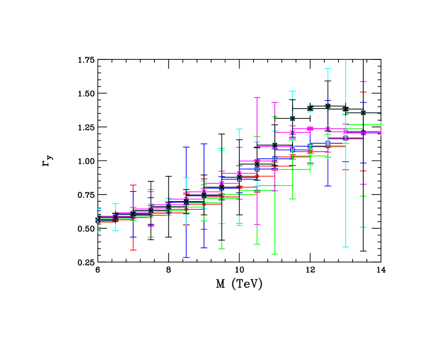
A third possible observable employing the dilepton final state is to construct rapidity ratio[4] in the region near the pole which is define via:
| (1) |
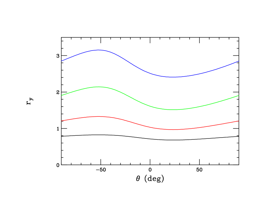
This ratio essentially measures the fraction of central rapidity events which depends upon the relative weighting of the and pdfs with the cut defining the central region boundary and . Note that as the mass increases for fixed the ratio will grow significantly due to the kinematic constraints arising from . For demonstration purposes, here we will assume but this value generally needs to be re-optimized for different values of the mass. To examine the sensitivity to coupling variations we present the results shown in Table 4 and Fig. 11 for various models and which employ the NWA. For low masses the sensitivity is seen to be rather modest but increases significantly as the mass increases. Of course the available statistics to make this measurement decreases significantly for large masses and the statistical error on scales as where is the total number of relevant signal events. For example, this would imply, for a with a mass of 10 TeV, that for the SSM() case assuming a luminosity of 5 ab-1 whereas for a mass of 15 TeV we would instead obtain the values , respectively. Clearly there is some rather modest model sensitivity obtainable using this observable for relatively low masses. We could try getting more information by looking at as a function of the dilepton invariant mass, , but as Fig. 10 shows the overall behavior of this quantity is much more driven by the the shrinking rapidity range (for a fixed cut) as increases than by the couplings.
| Model | 5 TeV | 10 TeV | 15 TeV | 20 TeV |
|---|---|---|---|---|
| SSM | 0.725 | 1.060 | 1.655 | 2.561 |
| LRM | 0.740 | 1.096 | 1.713 | 2.625 |
| 0.712 | 1.033 | 1,612 | 2.513 | |
| 0.783 | 1.206 | 1.905 | 2.851 | |
| 0.691 | 0.987 | 1.542 | 2.438 | |
| I | 0.825 | 1.328 | 2.142 | 3.153 |
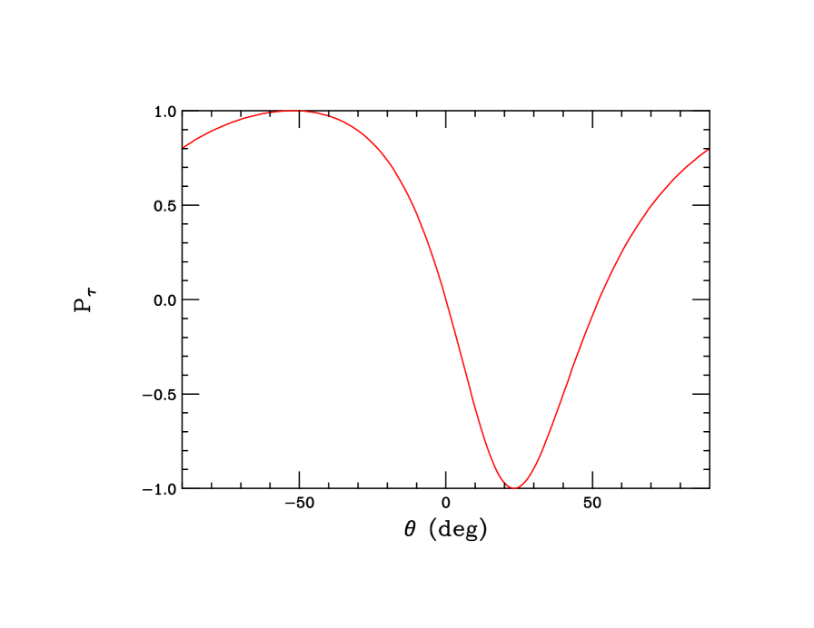
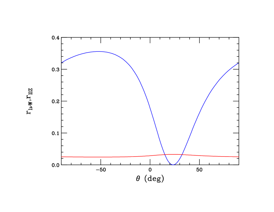
As a last possibility worth mentioning, one can imagine employing the ditau decay mode of the and then measure the polarization of the ’s themselves[4]. The lower panel in Fig. 11 shows that this quantity, if measurable, has quite significant coupling sensitivity. However, at the 100 TeV FHC, performing this measurement using, e.g., the or decays from the may prove to be rather difficult given the rather complex hadronic environment one might naively expect. However this is certainly worthy of further study.
As discussed above, here we have been limiting our discussion to signals employing leptonic triggers so that we will not consider modes such as . Thus we are led to consider 3-body decays involving leptons such as and and, in particular the ratios of the partial widths for these reactions relative to that for denoted as and in the literature[4]. As discussed above, we employ these ratios to remove the potential sensitivity to non-SM decays. Assuming that the coupling is absent at tree-level (which it is in the GUT-type models under consideration in the absence of mixing which we assume here), these processes occur by the emission of gauge bosons from one of the lepton legs in ordinary dilepton decays. At the LHC, for masses TeV, these ratios were shown to be useful for coupling determinations but suffered from small statistics. We note in Fig. 12, however, that (and similarly ) grow like due to the near infrared and co-linear sigularities in the relevant graphs. This renders them potentially far more useful than at lower collision energies although clearly should be the focus of our attention. For example, for a mass of 15 TeV in the LRM the cross section for the final state is ab. One difficulty at these energies is the rather large boost of the final state and its small opening angle with respect to the lepton from which it was emitted, i.e., isolation issues. Further, if the are found through their dijet decay modes these two jets will not allow for separation and will also likely appear as a single jet. This final state warrants further study at the FHC.
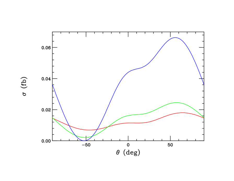
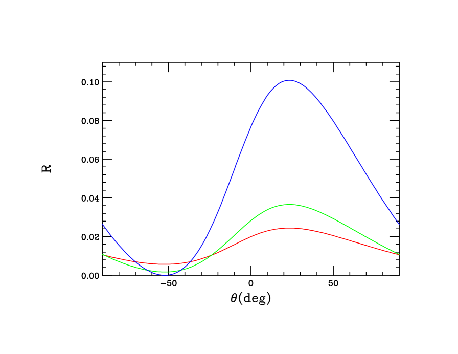
As a final potential probe of couplings, we can consider the cross sections for the associated production of the , observed via its leptonic decay mode as usual, together with some other SM gauge field, a high-, or [4] produced via ‘initial state radiation’. Scaling these cross sections to that for ordinary production yields a set of observables, , that are immune to the possible existence of non-SM decay modes. Fig. 13 shows both the production cross sections for these final states as well as the associated ratios assuming a 10 TeV mass at the 100 TeV FHC. Note that in the case, a cut of 100 GeV has been applied to the final state photon. (The above comments about the and final state identification in dijets will also apply here as well.) These results show that the associated production observables will suffer from somewhat low statistics if only ab-1 of integrated luminosity is available at the FHC but they still warrant further study at the FHC.
3 New Bosons
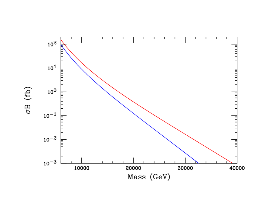
We now turn our attention to new gauge bosons which are generally far less well studied than are the . As in the case the first issue to address is the production cross section at the 100 TeV FHC; as for the we limit ourselves to final states involving lepton tags so that the primary discovery channel is with the appearing as a large amount of MET. All calculations for the will be performed in the same manner as in the case above making use of the same inputs and assumptions.
Here we face an immediate issue: in essentially every model in the literature the couplings of the to SM fermions are either purely LH or RH. Assuming that neutrinos are either Dirac fermions or are light and detector-stable Majorana fermions, so that this same final state occurs in both cases and that, apart from phases, the RH and LH CKM mixing matrices are the same (which is a likely occurrence in, e.g., the LRM) then in the NWA limit the production cross section is independent of this helicity choice[18]. The resulting cross section is shown in Fig. 14 for both and 100 TeV for comparison purposes. Here we can observe several things (that will be seen in more detail below): () At GeV the discovery reach is TeV while () the CL exclusion limit is found to be 26.6(35.5) TeV. If the integrated luminosity is increased by a factor of 3(10) these numbers all increase by roughly 3.6(7.5) TeV. () At 100 TeV, if exotic modes are present to reduce the leptonic branching fraction by a factor of 2, then the corresponding discovery reach is reduced by TeV. It is important to remember that since the couplings are either LH or RH, determining which of these is realized is the primary goal after the discovery777As discussed above we only consider leptonic modes here;see however[19], [20] and [21] for other possibilities .
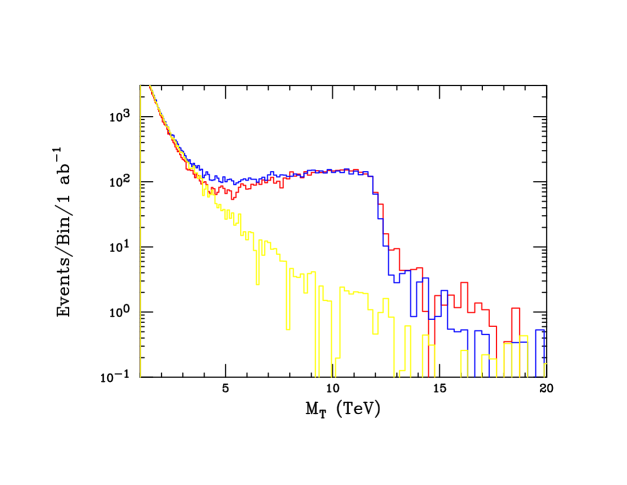
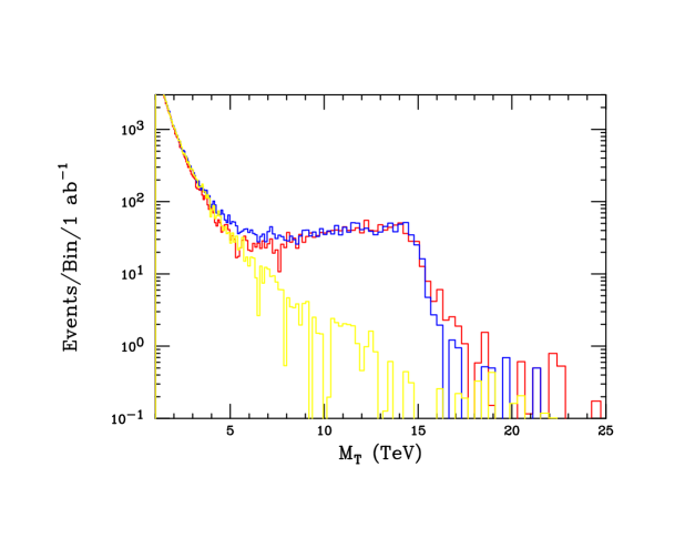
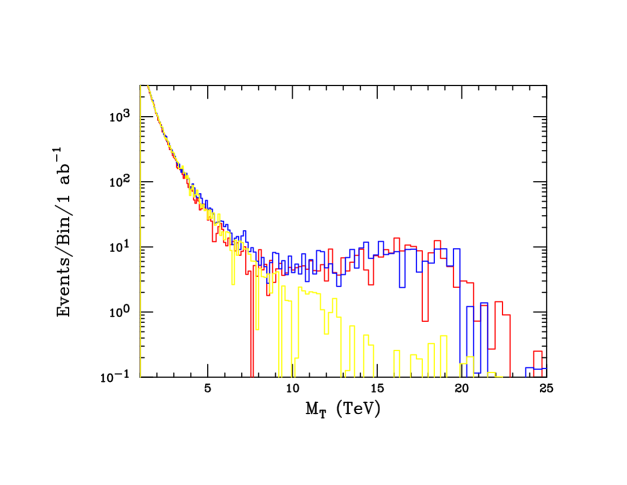
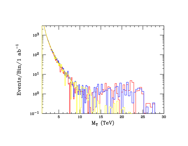
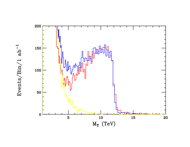
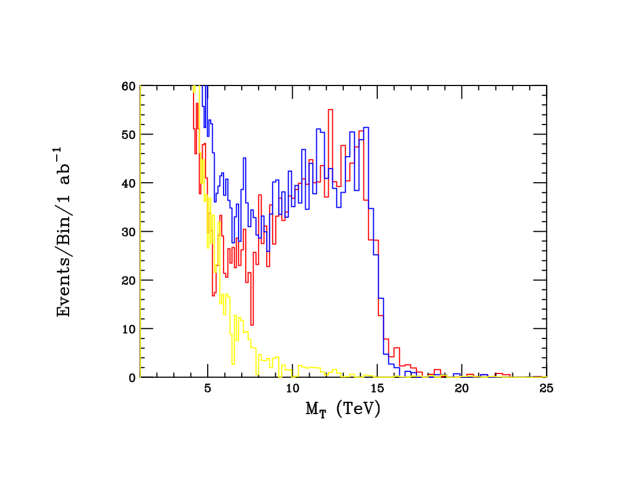
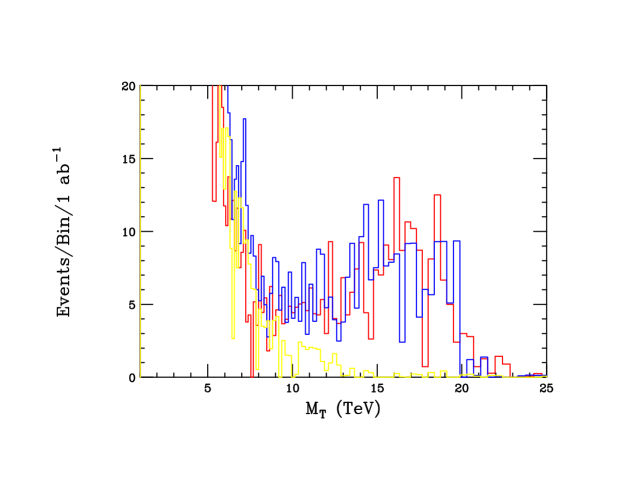
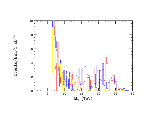
Of course the actual way that a would be discovered would be via the observation of an excess in the number of events at the high end of the transverse mass () distribution formed from the charged lepton and the MET as in the case of the SM . (Here we will need to assume that the FHC detector(s) can easily identify large amounts of MET with ATLAS-like resolution.) To this end it is instructive to examine these distributions for different values of the mass assuming either LH or RH couplings to the usual SM fermions. The results for masses of 12, 15, 20 and 25 TeV are shown in Figs. 15 and 16 on log and linear scales respectively888Here we display both log and linear scale event rate plots as we can learn something from both of these projections.. Several things are immediately apparent: () the for all these masses, whether LH or RH, is clearly visible above the SM background in a statistically significant way. () The behavior of the distribution in the neighborhood of the Jacobian peak is the same (within statistics) whether the is LH or RH. This conforms with our expectations from the NWA analysis above. () The overall shapes of the distributions for the LH and RH couplings are not the same[18] and CMS[10] in particular has exploited this fact as part of their search. This difference is particularly noticeable in two regions: for and above the Jacobian peak. In the lower mass region we see that the LH result lies below the RH one whereas above the Jacobian peak the reverse is true. This difference is due to the interference (or lack thereof) between the and the SM amplitudes. In the LH case, these amplitudes have opposite signs below the Jacobian peak but add constructively above it. In the RH case, however, there is no interference with the SM amplitude since the SM fermions in both the initial and final states are treated as massless. It is clear from these Figures that this difference in the distributions is apparently visible (at this assumed integrated luminosity) for masses possibly as large as TeV and may be potentially so even for somewhat larger masses even though all these values are still significantly below the corresponding discovery reach. Clearly no difference would be observable for a mass of 30 TeV although an excess of events would still be seen in both helicity cases. To get a clearer idea of the size of this cross section difference due to the coupling helicity (since the Figures can be sometimes misleading due to the small bin size) let us first imagine that a has been seen at a given mass through its Jacobian peak. One can then just count the total number of events in the distribution in the region where the interference is most important, , say, and compare the expectations in the two cases. For a LH(RH) with a mass of 12 TeV and an integrated luminosity of 1 ab-1 one obtains 8153(9818) events which certainly differ by more than (statistical errors only). Similarly, for masses of 15, 20 and 25 TeV, one correspondingly obtains 2669(3319), 592(771) and 175(208) events, respectfully, indicating good separation up to masses of TeV for these two coupling helicities. Of course, increased integrated luminosity will clarify only these issues further.
Although the shape of the distribution is a powerful probe of the handedness ( for LH(RH) couplings) of the , it would very useful to have other observables available to also determine this quantity. In the discussion above we saw that was a useful tool to get at the corresponding couplings. Here, since the SM fermions couple to the as , the corresponding asymmetry on the pole in the NWA would behave as
| (2) |
which trivially gives the same result for both helicities and is thus useless for present purposes. Again, as in the case, one might attempt to measure the polarization of the in but it is likely to be even more difficult in this case due to the additional MET and busy detector environment. Building further on our experience we could try to examine both the associated production process (which would likely have contamination if is used) or the rare bremsstrahlung-like decay (here cutting away the pole region) for helicity sensitivity. Naively, if the were purely RH both these processes would be absent at tree-level so that just their simple observation would inform us that the is LH. However, since a traditional only arises from an additional group factor, it is always accompanied by a due to gauge invariance so that vertices such as and/or might be present which will not necessarily turn on or off depending upon the helicity of the coupling to the SM fermions999However, as discussed in detail in Ref. [18], there are no known models with a RH where these potentially dangerous vertices are not suppressed by gauge boson mixing angles.. Thus some care would be required in interpreting the observation of either of these processes and they both warrant further investigation.
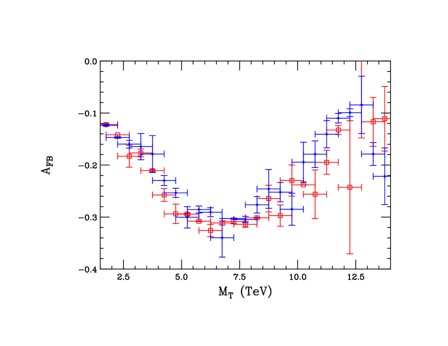
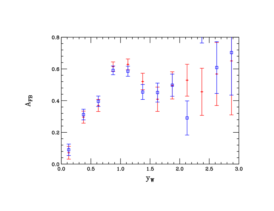
Since these NWA-like processes do not appear to be very promising, we turn to a number of asymmetry distributions that one can form using the MET discovery mode of the . Since we already know about the possible interference as a probe of the coupling helicities it is worthwhile to take advantage of this. Although we’ve shown that near the Jacobian peak region is insensitive to this helicity choice we might wonder if we can learn something by examining lower values where this interference is certainly most relevant. The asymmetry predictions for and for are found to be slightly different (due to the pdfs) but here we combine them, weighted by their associated cross sections, to increase statistical sensitivity while still integrating over the rapidity. As in the case we impose a minimum rapidity cut here in an attempt to define the initial quark direction so that the angle can be determined. We assume, as we did in the case, that a mis-identification of this angle can be corrected for statistically using Monte Carlo. The top panel of Fig. 17 show the results of this calculation for employing 5 ab-1 and a relatively light of mass 12 TeV. Clearly there seems to be very little power here to resolve the LH vs. RH dichotomy with this level of statistics. Alternatively we can focus on the expected interference region, here taking in the 3-9 TeV range and examine the rapidity dependence of the distribution of the itself. Since this distribution is odd in we fold it over to increase statistics. We also can again combine the results for and by a sign flip and event weighting to increase the statistics even further. Unfortunately, as the lower panel of Fig. 17 shows, this observable assuming even this large value of the integrated luminosity cannot distinguish between the two helicity possibilities even for a relatively light of mass 12 TeV.
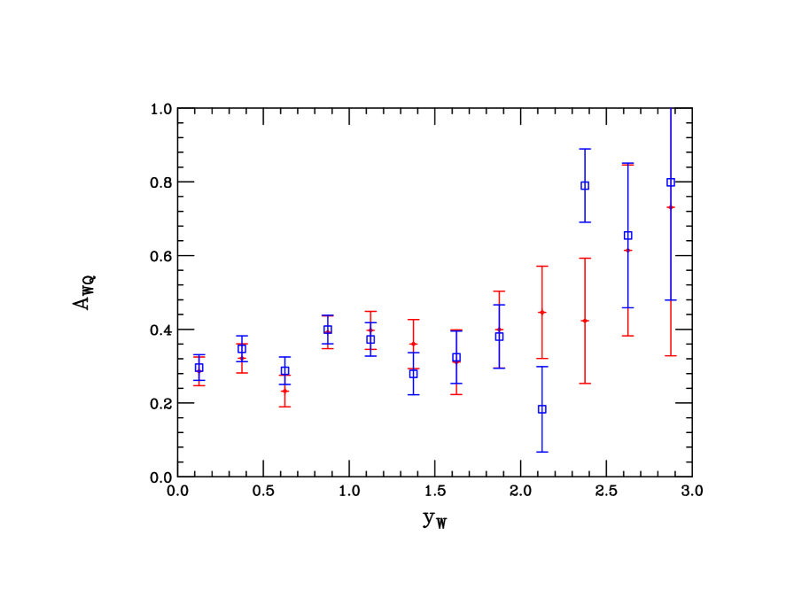
There still remains other asymmetries which we can form with this same final state: we first consider is the charge asymmetry, :
| (3) |
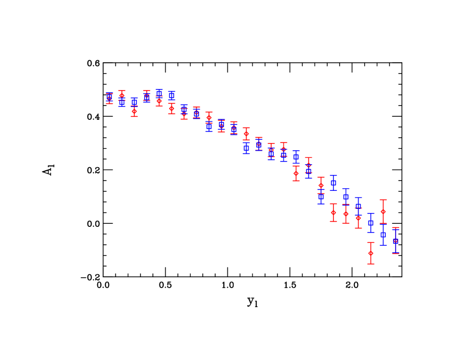
where are the number of events with s of a specific charge in given rapidity bin. Note that at pp colliders, is symmetric under so that we can again fold the distribution around to increase statistics. The upper panel in Fig. 18 shows this distribution, integrated over the interference region TeV, assuming TeV and assuming a luminosity of 5 . It is clear that at this level of statistics the two distributions are reasonably indistinguishable. As a final asymmetry possibility, we consider is the rapidity asymmetry for the final state charged leptons themselves, :
| (4) |
which is an even function of so that this asymmetry too can be folded around . The resulting distribution can be seen in the lower panel of Fig. 18 for the same mass and integrated luminosity. Here we again see hardly any model differentiation between the two helicity choices.
From this general discussion of possibly asymmetries that one can form employing this leptonic final state we can conclude that their overall usefulness in coupling helicity determination will require very high integrated luminosities beyond the 5 ab-1 employed in this survey unless the is significantly lighter than our 12 TeV test example (by at least a few TeV). Clearly the shape of the distribution appears to be the lone observable employing ‘modest’ statistics that will be available to determine the coupling helicity.
4 Conclusions
and production are standard benchmarks for study of the physics capabilities of any new collider. In this paper, we have examined the production properties of these new particles at the FHC, in particular, with eye towards understanding its ability to explore their couplings to the usual SM fermions. This is a necessary first step in uncovering the underlying theory from which such new particles might spring. Of course the FHC is a long way from where we are now and one needs to make extrapolations on the theoretical side (e.g., pdfs, etc) as well as make some guesses as to what objects might be well measured on the experimental side at such energies. For example, final states composed of purely hadronic objects or observables requiring b-tagging might be generally difficult to employ given the expected number of multiple interactions at 100 TeV with reasonable luminosities. Furthermore, it is likely that muon momenta in the multi-TeV range would be difficult to measure with high precision without enormous magnetic fields and/or bending radii. Here, we have assumed that electron energies (and to some extent MET for the case) can be as well measured by the FHC experiments as is presently done by the LHC experiments. Given these caveats, it is quite clear that the FHC will not only provide a huge step in the reach for these and states but will allow for a sufficient number of electron-based observables to be examined so that we can learn something substantial about their couplings to the SM. If multiple interactions could be dealt with and muon-based observables can also be employed, these conclusions will only be strengthened. It is not likely, however, that such information would be obtainable for new gauge boson masses which lie within TeV of the corresponding discovery reaches without significant luminosity increases after the fact (due to simple statistical limitations) or through the application of observables we have not considered here. In performing these studies we have employed a very familiar and long-used set of models with which we can make direct comparisons to other previous experimental and theoretical analyses. However, it is important to recall that this set, though somewhat representative of a more general class of theories, does not in any way span the full range of possibilities that experimenters might encounter at the FHC. Further study of new gauge boson physics at the FHC is certainly needed.
Clearly, much work will be required to understand what the full capabilities of the FHC might be. However, it is clear that the FHC would provide a giant step forward in the search for BSM physics and hopefully its construction will be realized sometime in the future.
Acknowledgments
The author would like to thank J.L. Hewett for discussions related to the work. He would also like to thank S. Godfrey for discussions about discovery reaches during the Snowmass meeting in Minneapolis. This work was supported by the Department of Energy, Contract DE-AC02-76SF00515.
Appendix
It is sometimes useful to ask what would happen to the discovery reach for and gauge bosons if their couplings differed from those in specified in a given model, particularly if they were weaker. To attempt to address this question here, we briefly consider the SSM gauge bosons but with couplings that differ in overall strengths than those discussed above. Extrapolation to larger couplings is rather straightforward as in the mass ranges of interest the signals remain in a region where there is essentially no (non-fake) SM backgrounds. This is of course no longer true when we consider weaker couplings and correspondingly smaller masses. In particular, once a region of low mass with significant SM background is reached one quickly becomes dominated by the systematic errors associated with our knowledge of this background due to the large integrated luminosities that we consider. This is certainly a subject worthy of some detailed study by the future FHC experimental collaborations as this relies on more of the detailed properties of possible detectors than is within the scope of the present work. If we assume that these backgrounds can be controlled and understood at the same level of uncertainty as claimed by ATLAS and CMS for the HL-LHC[12], then we can get an estimate of what the discovery reach might be for these states with weaker couplings. To get an idea of what might be possible at the FHC we will make this assumption below for the dilepton invariant mass region above a few TeV.
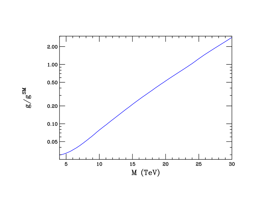
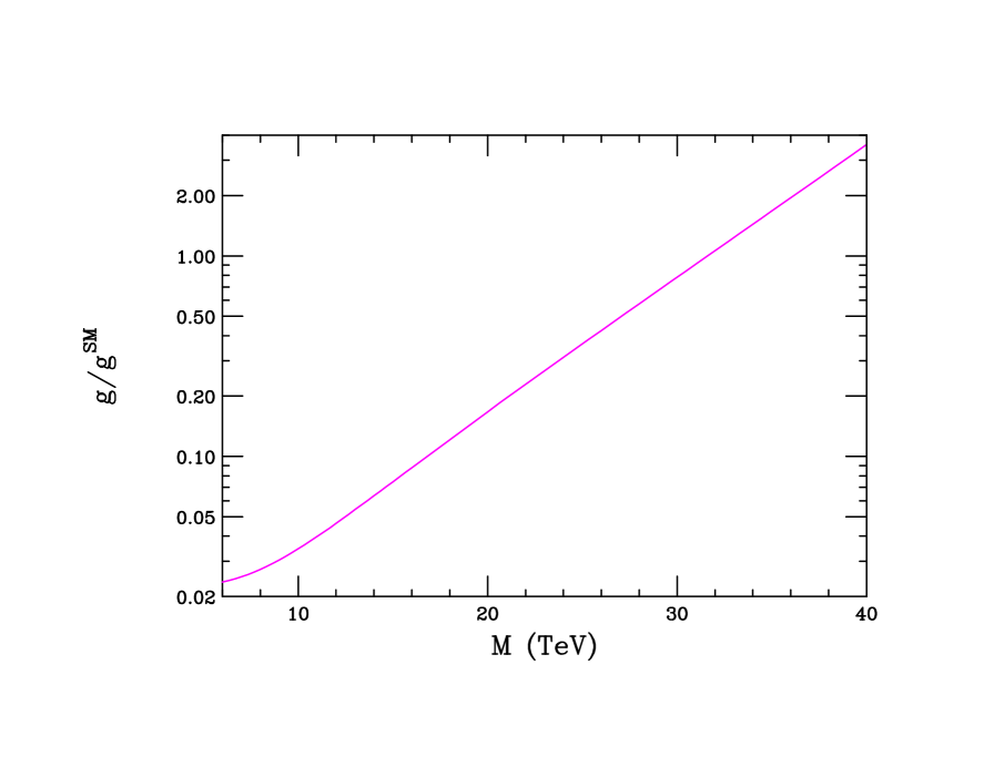
Following this approach we obtain the results as shown in Fig. 19 for both the SSM and with scaled couplings. In the case, we see that for the discovery reach for 1 ab-1 is reduced to TeV. In the corresponding case we see that the discovery reach is reduced to TeV. In both cases we note that at very low masses and small relative couplings the search reaches ‘saturate’ in the sense that smaller couplings cannot be probed with this level of systematic error given our rather simplified approach. This happens for masses below TeV, with corresponding couplings less than , in the case of the and at masses of TeV and the corresponding coupling below for the . We emphasize to the reader that these results are only approximate but do give us some indication of what might be achievable at the FHC.
References
- [1] See, for example, R. Brock, M.E. Peskin, et al., Snowmass Energy Frontier Group Report, http://www-public.slac.stanford.edu/snowmass2013/docs/Energy-3.pdf. There have also been and will be in the near future a number of workshops on the topic of an FHC; for an incomplete list see, for example LPC meeting on future 100 TeV proton collider, Fermilab, 31 January 2014, https://indico.cern.ch/event/294897/; BSM Physics Opportunities at 100 TeV, CERN, 10-11 February 2014, https://indico.cern.ch/event/284800/; CFHEP Symposium on Circular Collider Physics, IHEP, Beijing, 23-25 February 2014, http://indico.ihep.ac.cn/conferenceDisplay.py?confId=4068; Workshop on Physics at a 100 TeV Collider, SLAC, 23-25 April 2014, https://indico.fnal.gov/conferenceDisplay.py?confId=7633.
- [2] For details, see Future Circular Collider Study Kickoff Meeting, University of Geneva, 12-15 February 2014, http://indico.cern.ch/event/282344/.
- [3] G. Anderson, U. Baur, M. Berger, F. Borcherding, A. Brandt, D. Denisov, S. Eno and T. Han et al., hep-ph/9710254; U. Baur, R. Brock, J. Parsons, M. Albrow, D. Denisov, T. Han, A. Kotwal and F. Olness et al., eConf C 010630, E4001 (2001) [hep-ph/0201227]; M. G. Albrow, FERMILAB-VLHCPUB-147.
- [4] For some overviews of the physics of new gauge bosons and original references, see P. Langacker, Rev. Mod. Phys. 81, 1199 (2009) [arXiv:0801.1345 [hep-ph]]; M. Cvetic and S. Godfrey, arXiv:1307.7292, in *Barklow, T.L. (ed.) et al.: Electroweak symmetry breaking and new physics at the TeV scale* 383-415 [hep-ph/9504216]; J. L. Hewett and T. G. Rizzo, Phys. Rept. 183, 193 (1989); T. G. Rizzo, hep-ph/0610104.
- [5] S. Godfrey and T. Martin, arXiv:1309.1688 [hep-ph]; D. Hayden, R. Brock and C. Willis, arXiv:1308.5874 [hep-ex]; T. G. Rizzo, eConf C 960625, NEW142 (1996) [hep-ph/9609248]; S. Godfrey, eConf C 010630, P344 (2001) [hep-ph/0201093];
- [6] T. Han, P. Langacker, Z. Liu and L. -T. Wang, arXiv:1308.2738 [hep-ph].
- [7] [ATLAS Collaboration], ATLAS-CONF-2013-017.
- [8] G. Aad et al. [ATLAS Collaboration], Phys. Lett. B 701, 50 (2011) [arXiv:1103.1391 [hep-ex]].
- [9] CMS Collaboration [CMS Collaboration], CMS-PAS-EXO-12-061.
- [10] CMS Collaboration [CMS Collaboration], CMS-PAS-EXO-12-060; S. Chatrchyan et al. [CMS Collaboration], JHEP 1208, 023 (2012) [arXiv:1204.4764 [hep-ex]].
- [11] See the fourth paper in Ref. [4].
- [12] ATLAS Collaboration ATLAS Collaboration arXiv:1307.7292 [hep-ex]; CMS Collaboration CMS Collaboration arXiv:1307.7135 [hep-ex].
- [13] For a recent discussion, see B. Fuks, J. Proudom, J. Rojo and I. Schienbein, arXiv:1403.2383 [hep-ph].
- [14] P. M. Nadolsky, H. -L. Lai, Q. -H. Cao, J. Huston, J. Pumplin, D. Stump, W. -K. Tung and C. -P. Yuan, Phys. Rev. D 78, 013004 (2008) [arXiv:0802.0007 [hep-ph]].
- [15] K. Melnikov and F. Petriello, Phys. Rev. D 74, 114017 (2006) [hep-ph/0609070].
- [16] For a review and original references see R.N. Mohapatra, Unification and Supersymmetry (Springer, New York, 1986).
- [17] M. Schafer, F. Ledroit and B. Trocmé, ATL-PHYS-PUB-2005-010.
- [18] For a very detailed discussion and original references, see T. G. Rizzo, JHEP 0705, 037 (2007) [arXiv:0704.0235 [hep-ph]].
- [19] S. Gopalakrishna, T. Han, I. Lewis, Z. -g. Si and Y. -F. Zhou, Phys. Rev. D 82, 115020 (2010) [arXiv:1008.3508 [hep-ph]].
- [20] T. Han, I. Lewis, R. Ruiz and Z. -g. Si, Phys. Rev. D 87, 035011 (2013) [Erratum-ibid. D 87, no. 3, 039906 (2013)] [arXiv:1211.6447 [hep-ph]].
- [21] E. L. Berger, Q. -H. Cao, C. -R. Chen and H. Zhang, Phys. Rev. D 83, 114026 (2011) [arXiv:1103.3274 [hep-ph]].