On Poincaré cone property

Abstract

A domain $S\subset{\mathbb{R}}^{d}$ is said to fulfill the Poincaré cone property if any point in the boundary of $S$ is the vertex of a (finite) cone which does not otherwise intersects the closure $\bar{S}$. For more than a century, this condition has played a relevant role in the theory of partial differential equations, as a shape assumption aimed to ensure the existence of a solution for the classical Dirichlet problem on $S$. In a completely different setting, this paper is devoted to analyze some statistical applications of the Poincaré cone property (when defined in a slightly stronger version). First, we show that this condition can be seen as a sort of generalized convexity: while it is considerably less restrictive than convexity, it still retains some “convex flavour.” In particular, when imposed to a probability support $S$, this property allows the estimation of $S$ from a random sample of points, using the “hull principle” much in the same way as a convex support is estimated using the convex hull of the sample points. The statistical properties of such hull estimator (consistency, convergence rates, boundary estimation) are considered in detail. Second, it is shown that the class of sets fulfilling the Poincaré property is a $P$-Glivenko–Cantelli class for any absolutely continuous distribution $P$ on ${\mathbb{R}}^{d}$. This has some independent interest in the theory of empirical processes, since it extends the classical analogous result, established for convex sets, to a much larger class. Third, an algorithm to approximate the cone-convex hull of a finite sample of points is proposed and some practical illustrations are given.

, and t1Supported in part by Spanish Grant MTM2010-17366.

62G05, 62G20, Poincare property, Glivenko-Cantelli classes, set estimation

1 Introduction

The Poincaré cone property (PCP) is a regularity condition for sets in the Euclidean space. It has been used in mathematics (in partial differential equations and Brownian motion theory) since more than a century. We are concerned here with some new applications of this property in statistics and probability. Let us begin by formally establishing this condition, as well as other related notions we will use.

1.1 The Poincaré property: Some history

The standard version of PCP, which can be found in many books dealing with potential theory or Brownian motion is as follows; see, for example, Mörters and Peres mor10 , page 68:

Definition 1.

A domain $S\subset{\mathbb{R}}^{d}$ satisfies the Poincaré cone property at $x\in\partial S$ if there exist a cone $C(x)$ with vertex at $x$ and a number $h>0$ such that

$$C(x)\cap B(x,h)\subset S^{c},$$ (1)

where $B(x,h)$ denotes the open ball with center $x$ and radius $h$.

The interest of this property is mainly associated with the so-called Dirichlet problem which consist of finding a function $u$, harmonic on $S$ (i.e., $\nabla^{2}u=0$ on $S$) such that the restriction of $u$ to the boundary $\partial S$ coincides with a given continuous function $f$. This problem was posed by Gauss in 1840. During some years, it was believed (from a conjecture due to Gauss himself) that the problem had always a solution; however, this is not the case, unless some regularity assumptions are imposed on $S$. In 1899, Poincaré showed that a solution does exist whenever every point in $\partial S$ lies on the surface of a sphere which does not otherwise intersects the closure $\bar{S}$. In 1911, Zaremba showed that this “outer sphere condition” proposed by Poincaré could be weakened by replacing the sphere with a cone, as indicated in Definition 1. For this reason, condition (1) is sometimes also called Poincaré–Zaremba property (e.g., Gilbarg and Trudinger gil77 ) or just Zaremba’s condition (Karatzas and Shreve kar88 , page 250).

Further details on the use of this classical property, its history and its beautiful connections with the theory of Brownian motion can be found, for example, in Kellogg kel29 , Gilbarg and Trudinger gil77 , Karatzas and Shreve kar88 and Mörters and Peres mor10 .

The intuitive meaning of Definition 1 is quite clear: if, for a point $x\in\partial S$, we can always construct a “finite outside cone” $C(x)\cap B(x,h)$ with vertex $x$, then we are typically ruling out the existence of a sharp inward peak at $x$. A classical example of a set not fulfilling this condition is the so-called Lebesgue Thorn, which is expressively described as follows in Kellogg kel29 , page 285: Suppose we take a sphere with a deformable surface and at one of its points push in a very sharp spine (…). This set was first proposed by Lebesgue in 1913 as a counterexample to show that the Dirichlet problem is not always solvable.

1.2 From the Poincaré property to cone-convexity: Our main definitions

As established in Definition 1, the Poincaré cone property is pointwise in the sense that the opening angle $\rho$ of the cone $C$ and the radius $h$ of the ball $B(x,h)$ in the “$x$-cornet” $C(x)\cap B(x,h)$ of condition (1) might depend on $x$. For our statistical applications, we will need the condition (1) to hold uniformly in $x$. Also, we will not be restricted to assume that $S$ is a domain (i.e., an open connected set) since we are interested in using the Poincaré property for support of probability measures which, by definition, are closed sets.

So, in summary, the basic concepts we are going to handle arise as the following strengthened versions of Definition 1.

Definition 2.

We will say that the set $S\subset{\mathbb{R}}^{d}$ is $\rho$-cone-convex ($\rho$-cc), for some $\rho\in(0,\pi]$, if there exists $h>0$ such that for all $x\in\partial S$ there is an open cone $C_{\rho}(x)$ with opening angle $\rho$ and vertex $x$ such that the condition

$$C_{\rho}(x)\cap B(x,h)\subset S^{c},$$ (2)

holds. When the above condition is satisfied for a specified $h>0$ we will also say that $S$ is $\rho,h$-cone-convex.

In informal terms, we could compare this definition with the standard characterization of convex sets in terms of supporting hyperplanes: if the (closed) set $S$ is convex, then for each $x\in\partial S$ there is a supporting hyperplane $H=H(x)$ passing through $x$. Conversely, if $S$ is closed with nonempty interior, the existence of a supporting hyperplane for each $x\in\partial S$ implies that $S$ is convex. In Definition 2, we have replaced the supporting hyperplanes with “supporting cones” of the form $C_{\rho,h}(x)=C_{\rho}(x)\cap B(x,h)$. Thus, for $\rho=\pi$ and $h=\infty$, we would get as a particular case the hyperplane supporting property for convex sets. Observe, however, that $\rho$-cone convexity is a much more general condition than convexity as it allows the set $S$ to have holes and inward peaks, as long as they are not too sharp (the “sharpness” being limited by the angle $\rho$).

1.3 Applications to set estimation

We will explore here the applicability of Poincaré cone property from a completely different point of view, mostly related with the problem of set estimation  which basically deals with the reconstruction of a set $S$ from a random sample points. See, for example, Cuevas and Fraiman cue10 for an overview. Typically, in set estimation very little can be said about the target set $S$ (beyond some simple results of consistency) on the basis of the available sample information, unless some relatively strong shape restrictions are imposed on $S$. Of course such assumptions entail some loss in generality but, in return, a wealth of valuable results (estimation of the boundary and the boundary measure, rates of convergence, etc.) are typically obtained.

The convex case and the “hull mechanism.” The use we will make of the Poincaré condition, via $\rho$-cone-convexity, is better explained from the perspective of other more popular related properties. The most obvious one is convexity. If the support $S$ is assumed to be convex, then the natural estimator of $S$ from a sample $X_{1},\ldots,X_{n}$ is the convex hull $S_{n}(X_{1},\ldots,X_{n})$, that is the minimal convex set including the sample points. The study of the convex hull itself (even not considering its properties as an estimator of $S$) seems to be an inexhaustible subject of research in geometric probability: increasingly sophisticated results on the distributions of several random variables (number of vertices, area, perimeter, probability content, number of sides, etc.) associated with $S_{n}$ have been considered in the last fifty years. The survey paper by Reitzner rei10 provides an excellent up-to-date account of these topics.

The properties of the convex hull $S_{n}$ as an estimator of the support $S$, and in particular the convergence rates for the Hausdorff distance $d_{H}(S_{n},S)$, are studied by Dümbgen and Walther dum96 among others.

Thus, convexity is the prototypical example where the hull mechanism (that is to define our estimator as the “minimal one including the sample and fulfilling a desired shape property”) can be successfully used. It is natural to ask whether in other cases, under more general assumptions than convexity, the hull mechanism could also work.

From $r$-convexity to $\rho$-cone convexity. The so-called $r$-convexity property provides an interesting example: a closed set $S$ is said to be $r$-convex if it can be expressed as the intersection of a family of complements of balls with radius $r>0$. More precisely, $S$ is $r$-convex if and only if

$$S=\bigcap_{\{y:B(y,r)\cap S=\varnothing\}}B(y,r)^{c}.$$ (3)

It is easy to check that any convex set is also $r$-convex for all $r>0$ but, clearly, $r$-convexity is a much milder restriction. In particular, it allows for smooth or “round gulfs,” and even holes, in the set.

The study of this property dates back to Perkal per56 ; see also Walther wal97 for further statistical insights on this concept. From a statistical viewpoint, the interesting fact is that, if a set $S$ is assumed to be $r$-convex, then it can be (asymptotically) recovered from a random sample by just considering the $r$-convex hull of the data points as a natural estimator.

The effective calculation of this $r$-convex hull is much more involved than that of the ordinary convex hull. The R-package alphahull provides a practical implementation for the case $d=2$; see Pateiro-López and Rodríguez-Casal pat10 . Whereas the ordinary convex hull of a sample in the plane is always a polygon, the boundary of the $r$-convex hull is made of arcs of $r$-circumferences plus, perhaps, some isolated points; see Figure 4 in Section 7 for an example. More information on statistical properties, examples and applications of the $r$-convex hull can be found in Rodríguez-Casal rod07 , Pateiro-López and Rodríguez-Casal pat08 and Berrendero, Cuevas and Pateiro-López ber12 . Cuevas, Fraiman and Pateiro-López cue12 provide further results on the estimation of an $r$-convex support as well as also some insights regarding the comparison of $r$-convexity with other better known properties such as positive reach (Federer fed59 ) and the above mentioned (uniform) outer $r$-sphere property. In particular, $r$-convexity is shown to be slightly stronger than the “rolling” outer $r$-sphere property: for every point in the boundary of $S$ there exists a ball touching that point whose interior is included in $S^{c}$.

Figure 1: A general $\rho$-cone-convex set with inward peaks and holes.

In this paper, we replace the outer balls by “outer cones” (in the spirit of Poincaré’s definition). This led us in a natural way to the cone-convexity notion introduced in Definition 2. In a similar vein, expression (3) suggests the following cone-based analogue notion.

Definition 3.

A closed set $S\subset\mathbb{R}^{d}$ is said to be cone-convex by complement with parameters $\rho\in(0,\pi]$, $h>0$ ($\rho,h$-ccc) if and only if

$$S=\bigcap_{\{y:C_{\rho,h}(y)\cap S=\varnothing\}}\bigl{(}C_{\rho,h}(y)\bigr{)}^{c},$$ (4)

where $C_{\rho,h}(y)$ denotes a finite cone with vertex $y$, of type $C_{\rho,h}(y)=C_{\rho}(y)\cap B(y,h)$.

In informal terms, one could say that a closed set $S$ is convex by complement (with parameters $\rho$, $h$) if any point $x\notin S$ can be separated from $S$ by a finite cone $C_{\rho,h}(y)$, with opening angle $\rho$ and height $h$, which contains $x$.

Thus, in summary, the $\rho$-cone-convexity properties considered in this paper are two generalizations of the notion of $r$-convexity where the balls are replaced by finite cones; see Figure 1. These generalizations allow us to consider much more general sets with rougher boundaries. To be more precise, the cone convexity by complement is a direct extension of the notion of $r$-convexity, by replacing the balls of radius $r$ with the $\rho,h$-cones. Likewise, the $\rho,h$-cone-convexity is a generalization of the “outer rolling property” commented above (i.e., any boundary point of $S$ has a touching ball whose interior is included in $S^{c}$; see Cuevas, Fraiman and Pateiro-López cue12 for details). However, whereas the $r$-convexity implies the outer rolling ball property (see Proposition 2 in Cuevas, Fraiman and Pateiro-López cue12 ), the analogous implication does not hold for the cone-convex case: see Proposition 1 below.

We will show that, in spite of this gain in generality, the “hull principle” still works for the $\rho$-cone-convex properties, so that it can be also employed for estimation purposes. This means that a $\rho$-cc (or a $\rho$-ccc) support $S$ can be estimated, from a random sample drawn on $S$, just using the corresponding $\rho$-cone-convex hull of the sample points.

In addition, a relevant property (see Theorem 3) is also shown for the class of $\rho$-cone convex sets: whereas this class is considerably broader than that of convex sets, it is still a Glivenko–Cantelli class. This represents a generalization of the recent similar result proved by Cuevas, Fraiman and Pateiro-López cue12 for the case of $r$-convex sets. An application is given in Theorem 4.

1.4 Some notation. The organization of this paper

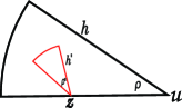
With some notational abuse, a “cornet” obtained by intersecting an infinite cone with a ball centered at its vertex is called itself as a (finite) cone. A set of this type is thus defined by the vertex $x$, a unit vector $\xi$ indicating the axis of the cone, an angle $\rho\in(0,\pi]$ indicating the opening angle and a positive number $h>0$ corresponding to the radius of the intersecting ball.

Thus, in precise terms, an infinite cone is defined by

$$C_{\rho}(x)=\biggl{\{}z\in{\mathbb{R}}^{d},z\neq x\dvtx\biggl{\langle}\xi,\frac{z-x}{\|z-x\|}\biggr{\rangle}>\cos(\rho/2)\biggr{\}},$$

and, for $h>0$, we will denote $C_{\rho,\xi,h}(x)=B(x,h)\cap C_{\rho}(x)$. The subindices, especially $\xi$, will be omitted when convenient, so the notation $C_{\rho,h}(x)$ is often used for finite cones.

The class of nonempty compact sets $S\subset{\mathbb{R}}^{d}$ satisfying, for a given $h>0$, the $\rho$-cone-convex condition (2) established in Definition 2 will be denoted by ${\mathcal{C}}_{\rho,h}$.

Also, the class of nonempty compact sets $S\subset{\mathbb{R}}^{d}$ satisfying, for a given $h>0$, the $\rho$-ccc condition established in Definition 3 will be denoted by $\tilde{\mathcal{C}}_{\rho,h}$. If $x\in\mathbb{R}^{d}$ and $S\subset\mathbb{R}^{d}$, $S\neq\varnothing$, the distance from $x$ to $S$ is $d(x,S)=\inf\{\|x-s\|\dvtx s\in S\}$. The Lebesgue measure on ${\mathbb{R}}^{d}$ will be denoted by $\mu$. Given a bounded set $A\subset{\mathbb{R}}^{d}$ and $\varepsilon>0$, $B(A,\varepsilon)$ will denote the parallel set $B(A,\varepsilon)=\{x\in{\mathbb{R}}^{d}\dvtx d(x,A)\leq\varepsilon\}$. Note that, according to this notation, $B(\{x\},\varepsilon)$ coincides with the closed ball centered at $x$ with radius $\varepsilon$, not with the open ball $B(x,\varepsilon)$.

Given two compact nonempty sets $A,B\subset{\mathbb{R}}^{d}$, the Hausdorff distance or Hausdorff–Pompein distance between $A$ and $C$ is defined by

$$d_{H}(A,C)=\inf\bigl{\{}\varepsilon>0\dvtx\mbox{such that }A\subset B(C,\varepsilon)\mbox{ and }C\subset B(A,\varepsilon)\bigr{\}}.$$ (5)

The class $\mathcal{M}$ of compact nonempty sets of ${\mathbb{R}}^{d}$, endowed with the distance $d_{H}$ is known to be a complete separable metric space; see, for example, Rockafellar and Wets roc09 , Chapter 4. Moreover, any class of uniformly bounded subsets in such space is relatively compact with respect to $d_{H}$. So, any bounded sequence of compact nonempty subsets of ${\mathbb{R}}^{d}$ has a convergent subsequence. For a given Borel measure $\nu$, define also the pseudometric $d_{\nu}(A,C)=\nu(A\setminus C)+\nu(C\setminus A)$.

The rest of this paper is organized as follows. In Section 2, we analyze the notions of “convex hulls” associated with the concepts of cone-convexity introduced above. Some general properties of convergence for sequences of cone-convex sets are obtained in Section 3. Section 4 is devoted to show that the class of cone-convex sets is a Glivenko–Cantelli class. This has some independent interest in the theory of empirical processes, since it extends the classical analogous result, established for convex sets, to a much larger class. The estimation (consistency and convergence rates) of cone-convex sets using the corresponding cone-convex hull of the sample is considered in Section 5. A stochastic algorithm to approximate the cone-convex hull by complement of a sample is provided in Section 6. The behavior of this algorithm is illustrated with some examples and simulations in Section 7. Some final comments and suggestions for further work are given in Section 8.

2 The notion of cone-convex hull

We now define the concept of cone-convex hull corresponding to the notion we have introduced of cone-convexity. In fact, we will need to distinguish between the “cone convex hull” and the “cone convex hull by complement” which, unlike the classical convex case, do not coincide in general for cone-convexity. Let $S\subset{\mathbb{R}}^{d}$ be a bounded set.

Definition 4.

(a) The $\rho,h$-cone-convex hull ($\rho,h$-cc) of $S$ or, just, the cone-convex hull of $S$, is defined by

$${\mathbb{C}}_{\rho,h}(S)=\bigcap_{S\subset B_{t},B_{t}\in\mathcal{C}_{\rho,h}}B_{t}.$$ (6)

[(b)]

The $\rho,h$-cone-convex hull by complement ($\rho,h$-ccc) of $S$, is defined as the intersection of the complements of those (open, finite) cones $C_{\rho,\xi,h}$ which do not intersect $S$. We will denote it by $\tilde{\mathbb{C}}_{\rho,h}(S)$. Note that $\tilde{\mathbb{C}}_{\rho,h}(S)$ can be also expressed as

$$\tilde{\mathbb{C}}_{\rho,h}(S)=\bigcap_{S\subset B_{t},B_{t}\in\tilde{\mathcal{C}}_{\rho,h}}B_{t}.$$ (7)

Proposition 1.

Given $\rho\in(0,\pi]$ and $h>0$, we have the following relations between the two classes $\mathcal{C}_{\rho,h}$ and $\tilde{\mathcal{C}}_{\rho,h}$ of cone-convex sets, introduced in Section 1.4, and the corresponding cone-convex hulls ${\mathbb{C}}_{\rho,h}(S)$ and $\tilde{\mathbb{C}}_{\rho,h}(S)$ defined for any bounded $S\subset{\mathbb{R}}^{d}$. [(a)]

Neither of the classes $\mathcal{C}_{\rho,h}$ and $\tilde{\mathcal{C}}_{\rho,h}$ is included in the other.

${\mathbb{C}}_{\rho,h}(S)\in\mathcal{C}_{\rho,h}$ and $\tilde{\mathbb{C}}_{\rho,h}(S)\in\tilde{\mathcal{C}}_{\rho,h}$.

If $\rho^{\prime}\leq\rho$ and $h^{\prime}\leq h$, then $\mathcal{C}_{\rho,h}\subset\mathcal{C}_{\rho^{\prime},h^{\prime}}$ and $\tilde{\mathcal{C}}_{\rho,h}\subset\tilde{\mathcal{C}}_{\rho^{\prime},h^{\prime}}$. Also,${\mathbb{C}}_{\rho^{\prime},h^{\prime}}(S)=S$ for all $S\in\mathcal{C}_{\rho,h}$ and $\tilde{\mathbb{C}}_{\rho^{\prime},h^{\prime}}(S)=S$, for all $S\in\tilde{\mathcal{C}}_{\rho,h}$.

Let $S\subset\mathbb{R}^{d}$ be bounded. For all $\rho\in(0,\pi]$ and $h>0$, let us define $h^{\prime}=h/2\sin(\rho/2)$, $\rho^{\prime}=(\pi-\rho)/2$ if $\rho>\pi/3$ and $\rho^{\prime}=\rho$ if $\rho\leq\pi/3$. Then $\tilde{\mathbb{C}}_{\rho,h}(S)\in\mathcal{C}_{\rho^{\prime},h^{\prime}}$. As a consequence, if $S$ is $\rho,h$-ccc, then it is also $\rho^{\prime},h^{\prime}$-cc.

(a) Let $S$ denote the closed unit ball in ${\mathbb{R}}^{2}$ and let $C$ be any (open) cone with vertex at the origin $(0,0)$, opening angle $\rho\in(0,\pi/2]$ and height $h<1/2$. Then it is readily seen that the set $S\setminus C$ belongs to $\tilde{\mathcal{C}}_{\rho,h}$ but not to $\mathcal{C}_{\rho,h}$ since condition (2) fails for all $x\in\partial C$, $x\neq(0,0)$.

Figure 2: An example for which the envelopes ${\mathbb{C}}_{\pi/4,3}(S)$ and $\tilde{\mathbb{C}}_{\pi/4,3}(S)$ do not coincide.

Also, the set $E=E_{1}\cup E_{2}\subset{\mathbb{R}}^{2}$ where $E_{1}$ is the graph of the function $f(t)=t^{2}$ on $t\in[0,1]$ and $E_{2}=\{(t,0)\dvtx 0\leq t\leq 1\}$ belongs to $\mathcal{C}_{\rho,h}$ for all $\rho\in(0,\pi/2]$, $h>0$ but $E\notin\tilde{\mathcal{C}}_{\rho,h}$ for any $\rho$.

There are also counterexamples of sets $S$ with nonempty interior such that $S\in\mathcal{C}_{\rho,h}\setminus\tilde{\mathcal{C}}_{\rho,h}$: let $S$ be union of the triangle $T$ with vertices $(1,0)$, $(1+s,s)$ and $(1+s,-s)$, where $s=(\sqrt{2}-1)/2$, plus the seven congruent triangles obtained from $T$ by applying a rotation around $(0,0)$ with angle $\pi/4$; see Figure 2.

This set is $\pi/4,h$-cone-convex for any $h$. However, the origin cannot be separated from $S$ by any cone $C_{\pi/4,3}(y)$ since any such cone should contain at least one of the vertices of the congruent triangles of $S$.

(b) By definition, we have

$${\mathbb{C}}_{\rho,h}(S)=\bigcap_{S\subset B_{t},B_{t}\in\mathcal{C}_{\rho,h}}B_{t}.$$

Given $x\in\partial{\mathbb{C}}_{\rho,h}(S)$ we want to find a $C_{\rho,h}(x)$ with $C_{\rho,h}(x)\subset{\mathbb{C}}_{\rho,h}(S)^{c}$. We have $B(x,1/n)\cap B_{t}\neq\varnothing$ for all $B_{t}$ such that $S\subset B_{t}$ and $B_{t}\in\mathcal{C}_{\rho,h}$. Moreover, $B(x,1/n)\cap B_{n}^{c}\neq\varnothing$ for some $B_{n}$ with $S\subset B_{n}$ and $B_{n}\in\mathcal{C}_{\rho,h}$. Given $z_{n}\in B(x,1/n)\cap\partial B_{n}$, we have $z_{n}\rightarrow x$. Since $z_{n}\in\partial B_{n}$ and $B_{n}\in\mathcal{C}_{\rho,h}$, there must exist a cone $C_{\rho,\xi_{n},h}(z_{n})\subset B_{n}^{c}$. Since $\|\xi_{n}\|=1$ there exists $\xi=\lim_{n}\xi_{n}$ (for some subsequence $\xi_{n}$) and also $z_{n}\rightarrow x$. We thus have that $\overline{C_{\rho,\xi_{n},h}(z_{n})}$ converges in the Hausdorff metric to $\overline{C_{\rho,\xi,h}(x)}$. We only must check $C_{\rho,\xi,h}(x)\cap S=\varnothing$. Indeed, otherwise we would have some $s\in S\cap C_{\rho,\xi,h}(x)$ with $\langle\frac{s-x}{\|s-x\|},\xi\rangle=\cos(\rho/2)+\delta$, for some $\delta>0$. Then $\langle\frac{s-z_{n}}{\|s-z_{n}\|},\xi_{n}\rangle>\cos(\rho/2)$, for $n$ large enough, which contradicts $C_{\rho,\xi,h}(z_{n})\cap S=\varnothing$.

The second statement follows directly from the expression (7).

(c) This is a direct consequence of the definitions of the classes and the respective hulls.

(d) We want to find $\rho^{\prime},h^{\prime}$ such that for any $z\in\partial\tilde{\mathbb{C}}_{\rho,h}(S)$ we have a cone $C_{\rho^{\prime},h^{\prime}}(z)$ with $C_{\rho^{\prime},h^{\prime}}(z)\subset\tilde{\mathbb{C}}_{\rho,h}(S)^{c}$. Now, take a sequence $z_{n}\to z$ with $z_{n}\in\tilde{\mathbb{C}}_{\rho,h}(S)^{c}$. Using the definition of $\tilde{\mathbb{C}}_{\rho,h}(S)$, there is a sequence of cones $C_{\rho,h}(u_{n})$, disjoint with $\tilde{\mathbb{C}}_{\rho,h}(S)$, such that $z_{n}\in C_{\rho,h}(u_{n})$. Take a further subsequence such that the cones $C_{\rho,h}(u_{n})$ are convergent, that is, $C_{\rho,h}(u_{n})\to C_{\rho,h}(u)$. By construction, we have that $z\in\partial C_{\rho,h}(u)$ and $C_{\rho,h}(u)\cap\tilde{\mathbb{C}}_{\rho,h}(S)=\varnothing$. It only remains to show that $C_{\rho^{\prime},h^{\prime}}(z)\subset C_{\rho,h}(u)$. This is readily seen for the given values of $\rho^{\prime}$ and $h^{\prime}$; see Figure 3. Indeed, the result is immediate for any $z$ at a distance $h/2$ from the vertex $x$. For the remaining $z\in\partial C_{\rho,h}(z)$ simple translations of this cone, perhaps combined with a rotation of the cone axis provide the required $C_{\rho^{\prime},h^{\prime}}(z)$.

Figure 3: For any $z\in\partial C_{\rho,h}(u)$ there is a cone $C_{\rho^{\prime},h^{\prime}}(z)\subset C_{\rho,h}(u)$.

Practical consequences in estimation problems. As a conclusion of the above result, we have two ways of estimating a cone-convex set $S$ from a sample $\aleph_{n}=\{X_{1},\ldots,X_{n}\}$ drawn from a distribution whose support is $S$. If we assume that $S$ is $\rho,h$-cone-convex, then the natural estimator of $S$ would be ${\mathbb{C}}_{\rho,h}(\aleph_{n})$. When $S$ is assumed to be $\rho,h$-cone-convex by complement, then $\tilde{\mathbb{C}}_{\rho,h}(\aleph_{n})$ would be the natural estimator of $S$.

The difference between both notions of cone-convexity is mainly technical. In fact, there is a considerable overlapping between the classes $\tilde{\mathcal{C}}_{\rho,h}$ and $\mathcal{C}_{\rho,h}$: most sets found in practice fulfilling one of these conditions will also satisfy the other one. For example, as pointed out above, if $S$ is $r$-convex (i.e., it can be expressed as the intersection of the complements of a family of $r$-balls), then $S$ fulfils both Definitions 2 and 3 of $\rho,r$-cone-convexity. In those cases, both envelopes ${\mathbb{C}}_{\rho,h}(\aleph_{n})$ and $\tilde{\mathbb{C}}_{\rho,h}(\aleph_{n})$ can be used.

We will analyze the asymptotic properties of both estimators, but the envelope $\tilde{\mathbb{C}}_{\rho,h}(\aleph_{n})$ is easier to approximate via an stochastic algorithm; see Section 6.

In practice, the correct choice of the parameters $\rho$, $h$ will depend on prior assumptions on the nature of the sets under study. Note, however, that result (c) in Proposition 1 guarantees that an exact knowledge of the “optimal” (maximal) values of these parameters is not needed, in the sense that a conservative (small) choice of $\rho$ and $h$ would do the job.

2.1 Lighthouses

A particular case of Definition 2 deserves attention as it represents a much more direct extension of the convexity notion: if condition (2) holds for all $h>0$ then, for each point in $\partial S$ we can find an infinite supporting cone on $x$. In this case, for $\rho=\pi$ condition (2) amounts to the supporting hyperplane condition. The formal definition would be as follows.

Definition 5.

We will say that $S$ is a $\rho$-lighthouse set when condition (2) holds for all $h>0$ or, equivalently, when for all $x\in\partial S$ there is an open cone $C_{\rho}(x)$ based on $x$ with opening angle $\rho$ such that

$$C_{\rho}(x)\subset S^{c}.$$ (8)

It is clear that the class ${\mathcal{C}}_{\rho}$ of compact sets in ${\mathbb{R}}^{d}$ fulfilling condition (8) is much broader than the class ${\mathcal{C}}$ of compact convex sets but, definitely, much smaller than any family ${\mathcal{C}}_{\rho,h}$ of $\rho,h$-cone-convex sets since condition (8) would typically exclude the presence of holes in $S$ [provided that $S=\overline{\operatorname{int}(S)}$]. In graphical terms, (8) imposes the possibility of illuminating the space around $S$ with a full beam of light from any boundary point $x$ in $S$. This accounts for the term “lighthouse.”

Likewise, the cone-convex hull notions introduced in Definition 4 can be readily adapted to the lighthouse sets just replacing the finite cones in both (6) and (7) by infinite (unbounded) cones.

In the next three sections, we will focus on the general case of $\rho,h$-cone-convex sets (for a finite $h$) but our results might be translated to the case of $\rho$-lighthouses. Apart from the simplicity and intuitive appeal of the lighthouse condition, the inference on the parameter $\rho$ is expected to be much easier in this case. However, this topic is not considered here.

3 Convergence properties

Let us start with a simple regularity property of cone-convex sets.

Proposition 2.

If $S\in{\mathcal{C}}_{\rho,h}$, then $\mu(\partial S)=0$.

First note that $\partial S$ is a Borel set since $S$ is closed. Now let us recall that a point $x\in S$ is said to have metric density 1 (see, e.g., Erdös erd45 ) if for all $\varepsilon>0$ there is some $\delta>0$ such that $\mu(S\cap B(x,r))>(1-\varepsilon)\mu(B(x,r))$ for all $r<\delta$. From Corollary 2.9 in Morgan mor00 , every set with positive (Lebesgue) measure has at least a point with metric density 1. This implies that we must have $\mu(\partial S)=0$ since for all $x\in\partial S$ there exists an open cone $C_{\rho,h}(x)\subset S^{c}$. Therefore, for all $r<h$, we have some $k_{\rho,h}<1$ such that

$$\mu\bigl{(}\partial S\cap B(x,r)\bigr{)} \leq \mu\bigl{(}S\cap B(x,r)\bigr{)}=\mu\bigl{(}S\cap C_{\rho,h}(x)^{c}\cap B(x,r)\bigr{)}$$

$$\leq k_{\rho,h}\mu\bigl{(}B(x,r)\bigr{)}.$$

We now establish that the convergence of a sequence of $\rho$-cone-convex sets entails the convergence of their respective boundaries. This is an important regularity property. It essentially says that we cannot have $\rho$-cone convex sets very close together if the respective boundaries are far away from each other. A similar property has been recently proved for sets fulfilling the rolling condition [i.e., property (1)] where $C(x)\cap B(x,h)$ is replaced by an open ball $B(x,r)$ of a given radius $r$, whose boundary contains $x$ (see Theorem 3(a) in Cuevas, Fraiman and Pateiro-López cue12 ; see also Baíllo and Cuevas bai01 for related results for the case of star-shaped sets). Our Theorem 1 below can be seen as a considerable extension of this result (since $\rho,h$-cone convexity is a much less restrictive than the rolling property).

Theorem 1.

Let $\{S_{n}\}\subset\mathcal{C}_{\rho,h}$ (or $\{S_{n}\}\subset\tilde{\mathcal{C}}_{\rho,h}$) and let $S\subset{\mathbb{R}}^{d}$ be a compact set such that $d_{H}(S_{n},S)\rightarrow 0$. Then $d_{H}(\partial S_{n},\partial S)\rightarrow 0$.

By contradiction, let us assume that $d_{H}(\partial S_{n},\partial S)\nrightarrow 0$. Then we should have either (i) or (ii): [(ii)]

There exists $\varepsilon>0$ such that for some subsequence $x_{n}\in\partial S$ we have $d(x_{n},\partial S_{n})>\varepsilon$.

There exists $\varepsilon>0$ such that for some subsequence $x_{n}\in\partial S_{n}$ we have $d(x_{n},\partial S)>\varepsilon$.

Suppose that we have a sequence $x_{n}$ fulfilling (i). Since $S$ is compact, there exists a convergent subsequence, denoted again $x_{n}$. Let $x$ be the limit of such subsequence. Since $d_{H}(S_{n},S)\rightarrow 0$, we have that, for $n$ large enough, $d(x,S_{n})\leq\varepsilon/2$. Moreover, taking the infimum on $y\in\partial S_{n}$ in $\|x_{n}-y\|\leq\|x_{n}-x\|+\|x-y\|$, we have that, eventually, $d(x,\partial S_{n})\geq d(x_{n},\partial S_{n})\!-\!\|x\!-\!x_{n}\|>\varepsilon/2$.

On the other hand, since $d(x,S_{n})\leq\varepsilon/2$ and $d(x,\partial S_{n})>\varepsilon/2$ we have $x\in\operatorname{int}(S_{n})$ and $B(x,\varepsilon/2)\cap S_{n}^{c}=\varnothing$. Since $x\in\partial S$ and $S$ is compact, we may take $y\in S^{c}$ such that $\|x-y\|<\varepsilon/2$ and $d(y,S)>0$. But $d_{H}(S_{n},S)\rightarrow 0$ and $d(y,S)>0$ entail $d(y,S_{n})>0$ eventually, so $y\in B(x,\varepsilon/2)\cap S_{n}^{c}$, in contradiction with $B(x,\varepsilon/2)\cap S_{n}^{c}=\varnothing$.

Let us now assume that we have (ii). Since $d_{H}(S_{n},S)\to 0$, we must have $d(x_{n},S)<\varepsilon$ eventually which, together with $d(x_{n},\partial S)>\varepsilon$, yields [by a similar reasoning to that in (i)] $x_{n}\in\operatorname{int}(S)$ eventually. Take now a convergent subsequence of $x_{n}$ (denoted again $x_{n}$) with $x_{n}\rightarrow x\in S$ and $d(x,\partial S)>\varepsilon/2$, that is, $B(x,\varepsilon/2)\subset S$. Since $x_{n}\in\partial S_{n}$ and $S_{n}\in\mathcal{C}_{\rho,h}$, there exist finite cones $C_{\rho,h}(x_{n})$ with $C_{\rho,h}(x_{n})\cap S_{n}=\varnothing$. Take $c_{n}\in S_{n}^{c}$, in the axis of $C_{\rho,h}(x_{n})$, with $0<\|x_{n}-c_{n}\|=\min\{h/2,\varepsilon/4\}=k$. We may assume (taking, if necessary, a further suitable subsequence) $c_{n}\rightarrow c$ and $\|c-x\|\leq\varepsilon/4$. Note that, by construction, $d(c_{n},S_{n})\geq k\sin(\rho/2)$. Hence, $d(c,S_{n})>k^{\prime}$ eventually, for some constant $k^{\prime}>0$. Since $d_{H}(S_{n},S)\to 0$, we must have $c\in S^{c}$, in contradiction with $c\in B(x,\varepsilon/2)\subset S$.

For the case $\{S_{n}\}\subset\tilde{\mathcal{C}}_{\rho,h}$, the result follows as a consequence of the previous case together with Proposition 1(d).

The following result shows that the class $\mathcal{C}_{\rho,h}$ is topologically closed.

Theorem 2.

Let $\{S_{n}\}\subset\mathcal{C}_{\rho,h}$ and let $S\subset{\mathbb{R}}^{d}$ be a compact set such that $d_{H}(S_{n},S)\rightarrow 0$. Then, $S\in\mathcal{C}_{\rho,h}$.

Given $x\in\partial S$, we want to find a finite cone $C_{\rho,h}(x)\subset S^{c}$. From Theorem 1, we know that $d_{H}(\partial S_{n},\partial S)\rightarrow 0$. Therefore, there is a sequence $x_{n}\in\partial S_{n}$ such that $x_{n}\rightarrow x$.

Now the reasoning to find a cone $C_{\rho,h}(x)$ is similar to that of Proposition 1. By considering, if necessary, a suitable subsequence of $x_{n}$, we may find again a sequence of finite closed cones $\{\overline{C_{\rho,\xi_{n},h}(x_{n})}\}$, with $C_{\rho,\xi_{n},h}(x_{n})\subset S_{n}^{c}$, converging in the Hausdorff metric to the closed cone $\overline{C_{\rho,\xi,h}(x)}$ for some direction $\xi$ with $\|\xi\|=1$. We now check that this is the cone we are looking for, that is, $C_{\rho,\xi,h}(x)\cap S=\varnothing$.

Suppose, by contradiction, that there is $z\in C_{\rho,\xi,h}(x)\cap S$. Since $\xi_{n}\rightarrow\xi$ and $x_{n}\rightarrow x$, we may take $\varepsilon>0$ such that for $n$ large enough $B(z,\varepsilon)\subset C_{\rho,\xi,h}(x_{n})$. This entails $d(z,S_{n})\geq\varepsilon$ infinitely often, which contradicts $d_{H}(S_{n},S)\to 0$.

4 The Glivenko–Cantelli property and the Poincaré condition

Let $X_{1},\break\ldots,X_{n},\ldots$ be a sequence of i.i.d., ${\mathbb{R}}^{d}$-valued random variables defined on a probability space $(\Omega,\mathfrak{F},\mathbb{P})$. Denote by ${P}$ the common distribution of the $X_{i}$’s on ${\mathbb{R}}^{d}$ and by $\mathbb{P}_{n}$ the empirical distribution associated with the first $n$ sample observations $X_{1},\ldots,X_{n}$.

The main result of this section will be established in Section 4.2 below. In order to view this result from an appropriate perspective, we next summarize some basic facts on the Glivenko–Cantelli (GC) property.

4.1 The Glivenko–Cantelli property: Some background

A class $\mathcal{A}$ of Borel subsets of ${\mathbb{R}}^{d}$ is said to be a $P$-Glivenko–Cantelli class whenever

$$\sup_{A\in\mathcal{A}}\bigl{|}\mathbb{P}_{n}(A)-{P}(A)\bigr{|}\rightarrow 0\qquad\mbox{a.s.}$$ (9)

These classes are named after the classical Glivenko–Cantelli theorem that establishes (9) for the case $d=1$ when $\mathcal{A}$ is the class of half-lines of type $(-\infty,x]$, with $x\in{\mathbb{R}}$.

In informal terms, a class $\mathcal{A}$ of sets is a GC-class if it is small enough as to ensure the uniform validity of the strong law of large numbers on $\mathcal{A}$. The study of GC-classes is a classical topic in the theory of empirical processes. See, for example, Shorack and Wellner sho86 and van der Vaart vaa98 , Chapter 19, for detailed accounts of this theory and its statistical applications. For example, Theorems 19.4 and 19.13 in van der Vaart vaa98 provide sufficient conditions for a class being $P$-Glivenko–Cantelli. These conditions are expressed in terms of entropy conditions which, in some sense, quantify the “size” of the class $\mathcal{A}$. Chapters 12 and 13 in the book Devroye, Györfi and Lugosi dev96 provide an insightful presentation of the Vapnik–Cervonenkis approach to the study of GC-classes. In that approach, the GC-property is obtained through an exponential bound for the probability ${\mathbb{P}}\{\sup_{A\in\mathcal{A}}|\mathbb{P}_{n}(A)-P(A)|>\varepsilon\}$. If the series (in $n$) of these bounds is convergent, then the classical Borel–Cantelli lemma, leads to (9). However, this approach fails for some important classes $\mathcal{A}$ as it requires the finiteness of the so-called Vapnik–Cervonenkis (VC) dimension of $\mathcal{A}$ (see Definition 12.2 in Devroye, Györfi and Lugosi dev96 ). A different approach, which can be used in fact for the study of GC-classes of functions is given by Talagrand tal87 . That approach can be used to establish the GC-property in some situations where the VC-dimension of $\mathcal{A}$ is infinite. Thus, it can be proved (as a consequence of Theorem 5 in Talagrand tal87 ) that, given a probability $P$ in ${\mathbb{R}}^{d}$, the class ${\mathcal{C}}$ of closed convex sets in ${\mathbb{R}}^{d}$ such that $P(\partial C)=0$ is a $P$-GC-class.

We shall use here a different, older approach to the GC-problem due to Billingsley and Topsøe bil67 . Billingsley–Topsøe approach can be used to prove a property called $P$-uniformity, which is in fact more general than the Glivenko–Cantelli condition, as it applies to general sequences of probability measures (not necessarily empirical measures). A class of sets $\mathcal{A}$ is said to be a $P$-uniformity class if

$$\sup_{A\in\mathcal{A}}\bigl{|}P_{n}(A)-P(A)\bigr{|}\to 0$$ (10)

holds for every sequence $P_{n}$ of probability measures converging weakly to $P$ (this is denoted $P_{n}\stackrel{{\scriptstyle w}}{{\rightarrow}}P$) in the sense that $P_{n}(B)\to P(B)$ for every Borel set $B$ such that $P(\partial B)=0$ [which of course happens, a.s. for $P_{n}=\mathbb{P}_{n}$; therefore, (10) implies (9)].

We will use a result in Billingsley and Topsøe bil67 , Theorem 4, according to which if $\mathcal{A}$ is a $P$-continuity class of Borel sets in ${\mathbb{R}}^{d}$ [i.e., $P(\partial A)=0$ for every $A\in\mathcal{A}$] then the compactness of the class $\{\partial A\dvtx A\in\mathcal{A}\}$, in the Hausdorff topology, is a sufficient condition for $\mathcal{A}$ to be a $P$-uniformity class.

In Theorem 5 of Cuevas, Fraiman and Pateiro-López cue12 , it is proved, using this result, that any class $\mathcal{A}$ of nonempty closed sets $A\subset{\mathbb{R}}^{d}$, uniformly bounded (i.e., all of them included in some common compact $K$) and fulfilling $\operatorname{reach}(A)\geq r$, for some given $r>0$, is a $P$-uniformity class whenever $P$ is a absolutely continuous with respect to the Lebesgue measure. Here, $\operatorname{reach}(A)$ denotes the supremum (possibly) of those values $s$ such that any point $x$ whose distance to $A$ is smaller than $s$ has just one closest point in $A$. The condition $\operatorname{reach}(A)>0$, introduced by Federer fed59 is a cornerstone in the geometric measure theory. This condition is a considerable generalization of the notion of convexity [as the convexity of $A$ is equivalent to $\operatorname{reach}(A)=\infty$ but a set with $\operatorname{reach}(A)>0$ can be highly nonconvex].

4.2 A Glivenko–Cantelli result for cone-convex sets

We will next establish a GC-result for the class ${\mathcal{C}}_{\rho,h}$ of nonempty compact sets fulfilling the $\rho,h$-cone-convex condition (2). In fact, we will establish the result for the larger class ${\mathcal{C}}^{U}_{\rho,h}$ of closed $\rho,h$-cone-convex sets (thus we may drop the boundedness condition). Since any closed convex set is in ${\mathcal{C}}_{\rho,h}^{U}$ we thus have an extension of the well-known GC-type result for the class of closed convex sets (see, e.g., Talagrand tal87 ). Also, the following result provides a strict generalization of Theorem 5 in Cuevas, Fraiman and Pateiro-López cue12 about the GC-property for sets with reach $\geq h$: indeed, note that, as established in that paper (Propositions 1 and 2), if a set fulfils reach $\geq h$ then the outer $h$-rolling property holds and hence the set belongs to the class ${\mathcal{C}}_{\rho,h}$ for $\rho<\pi/2$. Moreover, the boundedness assumption is dropped here. Similar comments and conclusions also hold for the class $\tilde{\mathcal{C}}^{U}_{\rho,h}$ of closed sets in ${\mathbb{R}}^{d}$ fulfilling the condition (4) of cone-convexity by complements. All this is summarized in the following result which will have some usefulness in the next section.

Theorem 3.

Let $\rho\in(0,\pi)$ and $h>0$. Let $P$ be a probability measure absolutely continuous with respect to the Lebesgue measure $\mu$. Then [(a)]

The class ${\mathcal{C}}^{U}_{\rho,h}$ of nonempty closed sets fulfilling the $\rho,h$-cone-convex condition (2) is a $P$-uniformity class (and in particular a $P$-Glivenko–Cantelli-class).

The same conclusion holds for the class $\tilde{\mathcal{C}}^{U}_{\rho,h}$ of closed sets fulfilling the condition (4) of cone-convexity by complements.

(a) Let us first establish the result for the subclass $\mathcal{A}\subset{\mathcal{C}}_{\rho,h}$ of sets in ${\mathcal{C}}_{\rho,h}$ included in a common compact set $K$. From Proposition 2, both ${\mathcal{C}}_{\rho,h}$ and $\mathcal{A}$ are $P$-continuous families. Given a sequence $\{A_{n}\}\subset\mathcal{A}$ there exist (since $\mathcal{A}$ is relatively compact in the space of compact sets endowed with the Hausdorff metric) a subsequence $\{A_{n_{k}}\}$ and a compact nonempty set $A$ such that $d_{H}(A_{n_{k}},A)\rightarrow 0$. From Theorem 2, $A\in\mathcal{C}_{\rho,h}$ and hence $A\in\mathcal{A}$. From Theorem 1, $d_{H}(\partial A_{n_{k}},\partial A)\rightarrow 0$. Therefore, the class $\partial\mathcal{A}=\{\partial A\dvtx A\in\mathcal{A}\}$ is compact in $\mathcal{M}$, thus fulfilling the above mentioned sufficient condition in Billingsley and Topsøe bil67 , Theorem 4. This entails the $P$-uniformity property for the class $\mathcal{A}$.

Finally, given $\varepsilon>0$ take a large enough $R$ such that $P(B(0,R)^{c})<\varepsilon/8$. Let $K=\overline{B(0,R)}$. If the weak convergence $P_{n}\stackrel{{\scriptstyle w}}{{\longrightarrow}}P$ holds we have, for large enough $n$, $P_{n}(K^{c})<\varepsilon/4$. Then, denoting ${\mathcal{C}}^{U}_{\rho,h}={\mathcal{D}}$,

$$\sup_{A\in{\mathcal{D}}}\bigl{|}P_{n}(A)-P(A)\bigr{|} \leq \sup_{A\in{\mathcal{D}}}\bigl{|}P_{n}(A\cap K)-P(A\cap K)\bigr{|}$$

$${}+\sup_{A\in{\mathcal{D}}}\bigl{|}P_{n}\bigl{(}A\cap K^{c}\bigr{)}-P\bigl{(}A\cap K^{c}\bigr{)}\bigr{|}$$

$$\leq \sup_{A\in{\mathcal{D}}}\bigl{|}P_{n}(A\cap K)-P(A\cap K)\bigr{|}+P_{n}\bigl{(}K^{c}\bigr{)}+P\bigl{(}K^{c}\bigr{)}<\varepsilon$$

for $n$ large enough, since $A\cap K$ belongs to the class $\mathcal{A}$.

(b) The result follows directly from (a) and from Proposition 1(d), which establishes that $\tilde{\mathcal{C}}_{\rho,h}\subset{\mathcal{C}}_{\rho^{\prime},h^{\prime}}$ for suitable values of $\rho^{\prime}$, $h^{\prime}$. Note also that, from Propositions 1(d) and 2, $\tilde{\mathcal{C}}_{\rho,h}$ is also a $P$-continuity class.

5 Estimation of cone-convex sets

This section is devoted to the study of the asymptotic properties of the two notions of cone-convex hull (when applied to a sample $\aleph_{n}$) given in Definition 4.

First, we obtain consistency and convergence rates for the $\rho,h$-cc estimator ${\mathbb{C}}_{\rho,h}(\aleph_{n})$. Second, we give convergence rates for the $\rho,h$-ccc convex hull $\tilde{\mathbb{C}}_{\rho,h}(\aleph_{n})$. Some key elements in the proof of the $\rho,h$-ccc case are the notion of unavoidable families (as in Pateiro-López and Rodríguez-Casal pat08 ) and some results on volume functions in Stachó sta76 .

5.1 Consistency and rates for the cone-convex hull

The following consistency result is a direct consequence of our GC-result (Theorem 3).

Theorem 4.

Let $P$ be a probability measure on ${\mathbb{R}}^{d}$, absolutely continuous with respect to the Lebesgue measure $\mu$. Assume that $P$ has a compact support $S$. Let $X_{1},\ldots,X_{n}$ be a sample drawn from $P$. Denote $\aleph_{n}=\{X_{1},\ldots,X_{n}\}$. [(a)]

If $S$ is $\rho,h$-cone convex, then the sequence ${\mathbb{C}}_{\rho,h}(\aleph_{n})$ of $\rho,h$-cone-convex hulls of $\aleph_{n}$ fulfills

$$d_{H}\bigl{(}{\mathbb{C}}_{\rho,h}(\aleph_{n}),S\bigr{)}\to 0\qquad\mbox{a.s.}\quad\mbox{and}\quad d_{\nu}\bigl{(}{\mathbb{C}}_{\rho,h}(\aleph_{n}),S\bigr{)}\to 0\qquad\mbox{a.s.}$$ (11)

for any measure $\nu$, finite on compact sets, whose restriction to $S$ is absolutely continuous with respect to $P$.

A similar result holds for the sequence $\tilde{\mathbb{C}}_{\rho,h}(\aleph_{n})$ of $\rho,h$-cone-convex hulls by complement, if we assume that $S\in\tilde{\mathcal{C}}_{\rho,h}$.

(a) The first result, $d_{H}({\mathbb{C}}_{\rho,h}(\aleph_{n}),S)\to 0$, a.s. is obvious since $d_{H}(\aleph_{n},S)\to 0$ a.s. and $\aleph_{n}\subset{\mathbb{C}}_{\rho,h}(\aleph_{n})\subset S$.

As for the second result, note that $d_{\nu}({\mathbb{C}}_{\rho,h}(\aleph_{n}),S)=\nu({\mathbb{C}}_{\rho,h}(\aleph_{n})\setminus S)+\nu(S\setminus{\mathbb{C}}_{\rho,h}(\aleph_{n}))$. The first term in the right-hand side is 0 a.s. As for the second one, since $\nu$ is absolutely continuous with respect to $P$ on $S$ and $S$ is the support of $P$, we only need to prove (from the well-known $\varepsilon$–$\delta$ characterization of absolute continuity, when $\nu$ is finite) that $P(S\setminus{\mathbb{C}}_{\rho,h}(\aleph_{n}))\to 0$, a.s. Indeed,

$$P\bigl{(}S\setminus{\mathbb{C}}_{\rho,h}(\aleph_{n})\bigr{)} = P(S)-P\bigl{(}{\mathbb{C}}_{\rho,h}(\aleph_{n})\bigr{)}$$

$$\leq \bigl{|}P(S)-{\mathbb{P}}_{n}\bigl{(}{\mathbb{C}}_{\rho,h}(\aleph_{n})\bigr{)}\bigr{|}$$

$${}+\bigl{|}{\mathbb{P}}_{n}\bigl{(}{\mathbb{C}}_{\rho,h}(\aleph_{n})\bigr{)}-P\bigl{(}{\mathbb{C}}_{\rho,h}(\aleph_{n})\bigr{)}\bigr{|}.$$

The first term is identically 0 a.s. The second one converges to 0 a.s. from Theorem 3(a).

(b) The proof of (b) is completely analogous using Theorem 3(b).

Remark 1.

A similar $d_{\nu}$-consistency result can be obtained by combining Theorem 1 above with Theorem 2 in Cuevas, Fraiman and Pateiro-López cue12 . However, Theorem 4 provides a more direct proof with an additional advantage: let us assume that $S$ belongs to a suitable subclass ${\mathcal{A}}\subset{\mathcal{C}}_{\rho,h}$, and the estimator $S_{n}$ is chosen in that class. If the convergence rate of $\sup_{A\in{\mathcal{A}}}|{\mathbb{P}}_{n}(A)-P(A)|$ is known, then from (5.1), the same convergence rate would immediately apply to $S_{n}$.

The following theorem provides convergence rates in the Hausdorff metric. Let us first recall (e.g., Cuevas and Fraiman cf97 ) that (taking the Lebesgue measure $\mu$ as a reference) a set $S\subset{\mathbb{R}}^{d}$ is said to be standard with respect to a Borel measure $\nu$ if there exist $\lambda>0$, $\delta>0$ such that

$$\nu\bigl{(}B(x,\varepsilon)\cap S\bigr{)}\geq\delta\mu\bigl{(}B(x,\varepsilon)\bigr{)}\qquad\mbox{for all }x\in S,0<\varepsilon\leq\lambda.$$ (14)

Theorem 5.

Assume that $X_{1},X_{2},\ldots,X_{n},\ldots$ are i.i.d. observations drawn from a distribution $P_{X}$ with support $S$. Assume also that $S$ is compact and standard with respect to $P_{X}$. Denote $\aleph_{n}=\{X_{1},X_{2},\ldots,X_{n}\}$. Then [(a)]

if $S\in\mathcal{C}_{\rho,h}$ then $d_{H}(\mathbb{C}_{\rho,h}(\aleph_{n}),S)=\mathcal{O}((\frac{\log n}{n})^{1/d})$ a.s.

The same conclusion holds for the estimator $\tilde{\mathbb{C}}_{\rho,h}(\aleph_{n})$ whenever the assumption $S\in\mathcal{C}_{\rho,h}$ is replaced with $S\in\tilde{\mathcal{C}}_{\rho,h}$.

(a) Let us first consider the case $S\in\mathcal{C}_{\rho,h}$. Since $\aleph_{n}\subset\mathbb{C}_{\rho,h}(\aleph_{n})\subset\mathbb{C}_{\rho,h}(S)=S$, the result follows directly from the following theorem given in Cuevas and Rodríguez-Casal cue04 , Theorem 3.

Let $X_{1},X_{2},\ldots$ be a sequence of i.i.d. observations drawn from a distribution $P_{X}$ on ${\mathbb{R}}^{d}$. Assume that the support $S$ of $P_{X}$ is compact and standard with respect to $P_{X}$. Then

$$\limsup_{n\rightarrow\infty}\biggl{(}\frac{n}{\log n}\biggr{)}^{{1}/{d}}d_{H}(\aleph_{n},S)\leq\biggl{(}\frac{2}{\delta\omega_{d}}\biggr{)}^{{1}/{d}}\qquad\mbox{a.s.},$$

where $\omega_{d}$ is the Lebesgue measure of the unit ball in ${\mathbb{R}}^{d}$ and $\delta$ is the standardness constant in (14) for $\nu=P_{X}$.

(b) The proof for the case $S\in\tilde{\mathcal{C}}_{\rho,h}$ is identical.

We will now study the rates of convergence for $d_{\mu}(\mathbb{C}_{\rho,h}(\aleph_{n}),S)$, with $S\in\mathcal{C}_{\rho,h}$.

We will need an assumption established in terms of the so-called $t$-inner parallel set of $S$, defined as $S\ominus tB(0,1)=\{x\in S\dvtx B(x,t)\subset S\}$. The inner parallel set appears as the result of applying the erosion operator $\ominus$ defined in the mathematical theory of image analysis; see Serra ser82 . Also, the inner parallel set has received some attention in differential geometry, on account of the regularity properties of its boundary; see Fu fu85 and Remark 3 below.

Theorem 6.

Let $S\subset{\mathbb{R}}^{d}$ fulfilling the assumptions of Theorem 5. Moreover, let us assume that

$$P_{X}\bigl{(}S\setminus S\ominus tB(0,1)\bigr{)}=\mathcal{O}(t).$$ (15)

Then, [(a)]

if $S\in\mathcal{C}_{\rho,h}$, $d_{P_{X}}(\mathbb{C}_{\rho,h}(\aleph_{n}),S)=\mathcal{O}((\frac{\log n}{n})^{1/d})$ a.s.

The same conclusion holds for the estimator $\tilde{\mathbb{C}}_{\rho,h}(\aleph_{n})$ if we assume $S\in\tilde{\mathcal{C}}_{\rho,h}$.

(a) Since $d_{P_{X}}(\mathbb{C}_{\rho,h}(\aleph_{n}),S)=P_{X}(S\setminus\mathbb{C}_{\rho,h}(\aleph_{n}))$, it suffices to show that if $\varepsilon_{n}=d_{H}(\aleph_{n},S)$, then there exists $k\in{\mathbb{R}}$ such that, with probability one, for $n$ large enough,

$$S\ominus k\varepsilon_{n}B(0,1)\subset\mathbb{C}_{\rho,h}(\aleph_{n}).$$ (16)

Indeed, in this case we would have (using again Cuevas and Rodríguez-Casal cue04 , Theorem 3)

$$P_{X}\bigl{(}S\setminus\mathbb{C}_{\rho,h}(\aleph_{n})\bigr{)} \leq P_{X}\bigl{(}S\setminus\bigl{(}S\ominus k\varepsilon_{n}B(0,1)\bigr{)}\bigr{)}$$

$$= \mathcal{O}(k\varepsilon_{n})=\mathcal{O}\biggl{(}\biggl{(}\frac{\log n}{n}\biggr{)}^{1/d}\biggr{)}\qquad\mbox{a.s.}$$

More precisely, we will show that (16) holds for $k=3+2/\sin(\rho/2)$. Choose $n_{0}=n_{0}(\omega)$ such that for $n>n_{0}$, $2\varepsilon_{n}/\sin(\rho/2)<h/2$. Now, by contradiction if there exists a sequence $x_{n}\in S\ominus k\varepsilon_{n}B(0,1)$ with $x_{n}\notin{\mathbb{C}}_{\rho,h}(\aleph_{n})$, we can find a sequence $B_{n}\in\mathcal{C}_{\rho,h}$ with $\aleph_{n}\subset B_{n}$ and $x_{n}\notin B_{n}$.

Since $\varepsilon_{n}=d_{H}(\aleph_{n},S)$, there exists $X_{i}\in\overline{B(x_{n},\varepsilon_{n})}$, but since $\aleph_{n}\subset B_{n}$ we also have $\overline{B(x_{n},\varepsilon_{n})}\cap B_{n}\neq\varnothing$ and $\overline{B(x_{n},\varepsilon_{n})}\cap B_{n}^{c}\neq\varnothing$. This entails the existence of $z_{n}\in\partial B_{n}$, $z_{n}\in\overline{B(x_{n},\varepsilon_{n})}$. Since $B_{n}\in\mathcal{C}_{\rho,h}$, we may choose a unit vector $\xi_{n}$ with $C_{\rho,\xi_{n},h}(z_{n})\subset B_{n}^{c}$ which implies $C_{\rho,\xi_{n},h}(z_{n})\cap\aleph_{n}=\varnothing$. Let us now consider $y_{n}=z_{n}+\frac{2\varepsilon_{n}}{\sin(\rho/2)}\xi_{n}$. If we prove $B(y_{n},2\varepsilon_{n})\subset S$, we have got a contradiction with $d_{H}(S,\aleph_{n})=\varepsilon_{n}$; indeed, from the definition of $y_{n}$ it is easy to see that $B(y_{n},2\varepsilon_{n})\subset C_{\rho,\xi_{n},h}(z_{n})\subset B_{n}^{c}$ so, as $\aleph_{n}\subset B_{n}$, one would have $B(y_{n},2\varepsilon_{n})\cap\aleph_{n}=\varnothing$. Now, in order to prove $B(y_{n},2\varepsilon_{n})\subset S$ recall that $B(x_{n},k\varepsilon_{n})\subset S$, so it suffices to check $B(y_{n},2\varepsilon_{n})\subset B(x_{n},k\varepsilon_{n})$, but if $t\in B(y_{n},2\varepsilon_{n})$, $\|t-x_{n}\|\leq\|t-y_{n}\|+\|y_{n}-z_{n}\|+\|z_{n}-x_{n}\|\leq 2\varepsilon_{n}+2\varepsilon_{n}/\sin(\rho/2)+\varepsilon_{n}=\varepsilon_{n}(3+2/\sin(\rho/2))$.

(b) The result follows from the above conclusion (a) and Proposition 1(d), since according to this result $\tilde{\mathbb{C}}_{\rho,h}(\aleph_{n})\in\mathcal{C}_{\rho^{\prime},h^{\prime}}$ so that

$${\mathbb{C}}_{\rho^{\prime},h^{\prime}}(\aleph_{n})\subset\tilde{\mathbb{C}}_{\rho,h}(\aleph_{n}).$$

Remark 2.

The convergence order obtained in Theorem 6 is the same found in Dümbgen and Walther dum96 for the case in which the ordinary notion of convexity for $S$ (and the convex hull for the estimator) are used, instead of the much more general concept of cone-convexity considered here. The same behavior is found in Rodríguez-Casal rod07 for the intermediate case in which $r$-convexity is assumed.

Remark 3.

Note that $S\setminus S\ominus tB(0,1)$ is the set of points in $S$ within a distance from $\partial S$ smaller than $t$. Thus, condition (15) has a clear intuitive interpretation, connected with some key concepts in Geometric Measure Theory. To begin with, let us recall that the erosion operator $\ominus$ provides (as well as the dual dilation operator $\oplus$) a well-known standard “smoothing” procedure in the mathematical theory of image analysis. Now, to give a more precise interpretation of condition (15) let us assume that $P_{X}$ is uniform, that is, proportional to the Lebesgue measure $\mu$ (similar conclusions can be drawn when $P_{X}$ fulfils $c_{1}\mu\leq P_{X}\leq c_{2}\mu$ for some constants $c_{1},c_{2}>0$). Note that, if we denote $T=S^{c}$, we have $S\setminus S\ominus tB(0,1)\subset B(T,t)\setminus T$. We thus have that (15) will hold whenever $\mu(B(T,t)\setminus T)=\mathcal{O}(t)$. A sufficient condition for this would be the celebrated Federer’s positive reach condition, a geometric smoothness notion introduced at the end of Section 4.1 above. More specifically, it is proved in Federer fed59 , Theorem 5.6, that if $\operatorname{reach}(\bar{T})=R$, then $\mu(B(T,t)\setminus T)$ is a polynomial in $t$, of degree $d$, for $t\in[0,R)$; in particular, (15) holds. Also, the finiteness of the outer Minkowski content of $T$ (defined by $L_{1}=\lim_{t\to 0}\mu(B(T,t)\setminus T)/t$; see Ambrosio, Colesanti and Villa amb08 ) is a sufficient condition for (15).

The following result shows that the boundary of $S$ can be estimated as well, with rates of the same order, under our cone-convexity assumption.

Corollary 1.

Under the assumptions of Theorem 6(a), we have that, with probability one, for $n$ large enough, $d_{H}(\partial S,\partial\mathbb{C}_{\rho,h}(\aleph_{n}))\leq kd_{H}(S,\aleph_{n})$, where $k=(3+2/\sin(\rho/2))$. A similar result holds for the $\rho,h$-ccc-hull $\tilde{\mathbb{C}}_{\rho,h}(\aleph_{n})$ if we assume the conditions of Theorem 6(b). In this case, the constant $k$ is replaced with $k^{\prime}=(3+2/\sin(\rho^{\prime}/2))$, where $\rho^{\prime}$ is the angle defined in Proposition 1(d).

In the case (a), the result follows from the content relation (16) together with $\partial{\mathbb{C}}_{\rho,h}(\aleph_{n})\subset S\setminus\operatorname{int}(S\ominus k\varepsilon_{n}B(0,1))\subset B(\partial S,k\varepsilon_{n})$ and the fact that, for any $x\in\partial S$ there is a sample point $X_{i}$ such that $\|x-X_{i}\|\leq\varepsilon_{n}$. Then, in the segment joining $x$ and $X_{i}$ there must be necessarily a point of $\partial{\mathbb{C}}_{\rho,h}(\aleph_{n})$. In the case (b), we use again $\mathbb{C}_{\rho^{\prime},h^{\prime}}(\aleph_{n})\subset\tilde{\mathbb{C}}_{\rho,h}(\aleph_{n})$ and Proposition 1(d).

5.2 Convergence rates in mean. Unavoidable families

We now focus on the convergence rates for the “mean error in measure” ${\mathbb{E}}d_{P_{X}}(\tilde{\mathbb{C}}_{\rho,h}(\aleph_{n}),S)$ where $P_{X}$ denotes the distribution of $X$. As we will see, the corresponding proof will involve some interesting methodological differences with the techniques used so far. In particular, relying on some ideas in Pateiro-López and Rodríguez-Casal pat12 , we will use the auxiliary notion of unavoidable families of sets which is next introduced and analyzed. Under suitable conditions ensuring $\mathcal{C}_{\rho,h}\subset\tilde{\mathcal{C}}_{\rho^{\prime},h^{\prime}}$, it should be possible also to obtain an analogous result for the cc-hull estimator ${\mathbb{C}}_{\rho,h}(\aleph_{n})$. However, this technical issue will not be considered here.

Unavoidable families of sets. Given $a\in(0,\pi)$ and $b>0$, denote ${\mathcal{G}}_{a,b}$ the family of all cones with opening angle $a$ and height $b$, that is, ${\mathcal{G}}_{a,b}=\{C_{a,\xi,b}(x)\dvtx\break x\in{\mathbb{R}}^{d},\|\xi\|=1\}$.

Definition 6.

A family of nonempty sets ${\mathfrak{U}}$ is said to be unavoidable for another family of sets $\Lambda$ if for each $L\in\Lambda$ there exists $U\in{\mathfrak{U}}$ with $U\subset L$.

The reason for using this notion here is as follows. Let $\Lambda_{\rho,h}(x)=\{C\in{\mathcal{G}}_{\rho,h}\dvtx x\in C\}$, that is, $\Lambda_{\rho,h}(x)$ is the family of $\rho,h$-cones which include the point $x$. Assume that we are able to find for each $x\in S$ a suitable finite family ${\mathfrak{U}}_{x,\rho,h}$, unavoidable for $\Lambda_{\rho,h}(x)$. Assume also that $X$ has a density $f$ satisfying $0<k_{1}\leq f(x)\leq k_{2}<\infty$ for almost all $x$ in $S$. We would then have

$$\mathbb{P}\bigl{(}x\in S\setminus\tilde{\mathbb{C}}_{\rho,h}(\aleph_{n})\bigr{)} = \mathbb{P}\bigl{(}\exists C\in\Lambda_{\rho,h}(x)\dvtx C\cap\aleph_{n}=\varnothing\bigr{)}$$

$$\leq \sum_{U\in\mathfrak{U}_{x,\rho,h}}\mathbb{P}(U\cap\aleph_{n}=\varnothing)\quad\mbox{and}$$

$$\mathbb{E}\bigl{(}d_{P_{X}}\bigl{(}S,\tilde{\mathbb{C}}_{\rho,h}(\aleph_{n})\bigr{)}\bigr{)} = \mathbb{E}\int_{S}\mathbb{I}_{\{x\in S\setminus\tilde{\mathbb{C}}_{\rho,h}(\aleph_{n})\}}f(x)\,dx$$

$$= \int_{S}\mathbb{P}\bigl{(}x\in S\setminus\tilde{\mathbb{C}}_{\rho,h}(\aleph_{n})\bigr{)}f(x)\,dx$$

$$\leq k_{2}\int_{S}\sum_{U\in\mathfrak{U}_{x,\rho,h}}\mathbb{P}(U\cap\aleph_{n}=\varnothing)\,dx$$

$$\leq k_{2}\int_{S}\sum_{U\in\mathfrak{U}_{x,\rho,h}}\bigl{(}1-k_{1}\mu(U\cap S)\bigr{)}^{n}\,dx,$$

where in the last inequality we have also used that $f$ is bounded from below. So, in order to find rates of convergence for ${\mathbb{E}}(d_{P_{X}}(S,\tilde{\mathbb{C}}_{\rho,h}(\aleph_{n})))$ the problem can be reduced to find, for each $x\in S$, a finite unavoidable family ${\mathfrak{U}}_{x,\rho,h}$ such that $k_{1}\mu(U\cap S)$ is large enough. Such families are described in the following proposition whose proof is given in the Appendix.

Proposition 3.

Let $\gamma=\rho$ if $\rho\leq\pi/3$ and $\gamma=(\pi-\rho)/2$ otherwise. Take $h_{1}=\frac{h}{2}\sin(\frac{\rho}{2})$. Given $x\in S$, consider a minimal covering of the closed ball $\overline{B(x,h_{1})}$ with closed cones of angle $\gamma/2$, axis $\xi_{j}$ and height $h_{1}$, $\{\overline{C_{\gamma/2,\xi_{j},h_{1}}(x)},\break\|\xi_{j}\|=1,j=1,\ldots,k\}$. Then the family

$${\mathfrak{U}}_{x,\rho,h}=\bigl{\{}C_{\gamma/2,\xi_{j},h_{1}}(x),\|\xi_{j}\|=1,j=1,\ldots k\bigr{\}},$$

is unavoidable for $\Lambda_{\rho,h}(x)$. Moreover, the cardinality of ${\mathfrak{U}}_{x,\rho,h}$ does not depend on $x$.

We now establish the main result of this section. Again the proof is given in the Appendix.

Theorem 7.

Let $S\subset{\mathbb{R}}^{d}$, $S\in\tilde{\mathcal{C}}_{\rho,h}$ and, for $z\geq 0$, $F(z)=\mu(\{x\in S\dvtx\break d(x,\partial S)\leq z\})$. Assume that $F^{\prime}$ is bounded in a neighborhood of 0, and $X_{1},X_{2},\ldots$ are i.i.d. drawn from a distribution $P_{X}$ with support $S$. Let us suppose that $P_{X}$ is absolutely continuous with $\mu$-density $f$ such that $0<k_{1}\leq f(x)\leq k_{2}<\infty$ for some constants $k_{1},k_{2}$ and for almost all $x\in S$. Then $\mathbb{E}(d_{P_{X}}(S,\tilde{\mathbb{C}}_{\rho,h}(\aleph_{n})))=\mathcal{O}(n^{-1/d})$.

Remark 4.

(a) Note that for any given compact set $S\subset{\mathbb{R}}^{d}$ with $\mu(\partial S)=0$, $F^{\prime}(0)$ the outer Minkowski content of $S^{c}$ (defined by $\lim_{\varepsilon\to 0}\frac{\mu(B(S^{c},\varepsilon)\setminus S^{c})}{\varepsilon}$). See Ambrosio, Colesanti and Villa amb08 for a deep study on this notion.

(b) The rate of convergence we have obtained is slower (when $d=2$) than the one obtained in Pateiro-López and Rodríguez-Casal pat12 (Theorem 1) for $r$-convex sets in ${\mathbb{R}}^{2}$, fulfilling a double rolling condition. In return, the class of cone-convex sets we are considering is much larger and we have no restriction on the dimension.

6 A stochastic algorithm for ccc-hulls

We offer here a relatively simple stochastic algorithm to approximately calculate the cone-convex hull by complement, $\tilde{\mathbb{C}}_{\rho,h}(\aleph_{n})$ for a given random sample $\aleph_{n}=\{X_{1},\ldots,X_{n}\}$.

As explained in Section 1.3, $\tilde{\mathbb{C}}_{\rho,h}(\aleph_{n})$ is a close analogue of the $r$-convex hull previously considered in the literature,

$$r\operatorname{conv}(\aleph_{n})=\bigcap_{\{y:B(y,r)\cap\aleph_{n}=\varnothing\}}B(y,r)^{c}.$$ (18)

An exact algorithm for the calculation of (18) for samples in ${\mathbb{R}}^{2}$ can be found in the R-package alphahull, described in Pateiro-López and Rodríguez-Casal pat10 .

The numerical treatment of the ccc-hull $\tilde{\mathbb{C}}_{\rho,h}(\aleph_{n})$ is a bit harder. This is essentially due to the lack of rotational symmetry of the “primary blocks” used in the construction of $\tilde{\mathbb{C}}_{\rho,h}(\aleph_{n})$, which are finite cones, instead of the balls of (18).

Our algorithm is based on the insightful heuristic description of (18) given in Edelsbrunner and Mücke edel94 : “Think of ${\mathbb{R}}^{3}$ filled with styrofoam and the points in $\aleph_{n}$ made of more solid material such as rock. Now imagine a spherical eraser with radius $r$. It is omnipresent in the sense that it carves out styrofoam at all positions where it does not enclose any of the sprinkled rocks, that is, points of $\aleph_{n}$. The resulting object will be called the $r$-hull.”

In our case, the “eraser element” is a finite cone $C_{\rho,h,\xi}(x)$ instead of a ball $B(x,r)$. So, in order to move the eraser we should in fact vary two parameters: the vertex $x$ and the axis direction $\xi$ (since the angle $\rho$ and the height $h$ remain fixed).

Our proposal is essentially based on the idea of choosing these two parameters with an “oriented random procedure”: we pick up randomly the vertex $x$ and then we erase as much styrofoam as possible by rotating the cone $C_{\rho,h,\xi}(x)$ for all directions $\xi$ with $C_{\rho,h,\xi}(x)\cap\aleph_{n}=\varnothing$. For $\theta\in[0,\pi/2]$, let us denote $R^{x}_{\theta}(u)$ the clockwise rotation of angle $\theta$ with center in $x$ of the vector $u$, (if $\theta\in[-\pi/2,0)$ we take the counter clockwise rotation). Then our algorithm is, in $\mathbb{R}^{2}$, as follows:

• INPUT: A sample $\aleph_{n}=\{X_{1},\ldots,X_{n}\}\subset{\mathbb{R}}^{2}$, the cone parameters $\rho\in(0,\pi]$ and $h>0$, a rectangle $E=[a,b]\times[c,d]$ with $\aleph_{n}\subset E$, $N$ a large positive integer indicating the number of full iterations of steps 1–3 below.

• STEP 1. Generating random cones: Choose at random a cone vertex $x\in E$ and a cone axis $\xi$ with $\|\xi\|=1$ and consider the cone $C_{\rho,h,\xi}(x)$.

• STEP 2. Checking for an empty cone: If $C_{\rho,h,\xi}(x)\cap\aleph_{n}\neq\varnothing$ go back to step 1.

• STEP 3. Erasing a maximal cone: If $C_{\rho,h,\xi}(x)\cap\aleph_{n}=\varnothing$ erase the maximal cone with vertex $x$ not containing any sample point. That is, find

  $$\theta_{0} = \max_{\theta\in[0,\pi/2]}\bigl{\{}\theta\dvtx C_{\theta/2,h,R^{x}_{\theta/2}(\xi)}(x)\cap\aleph_{n}=\varnothing\bigr{\}},$$

  $$\theta_{1} = \min_{\theta\in[-\pi/2,0)}\bigl{\{}\theta\dvtx C_{\theta/2,h,R^{x}_{\theta/2}(\xi)}(x)\cap\aleph_{n}=\varnothing\bigr{\}}.$$

  Then erase the $h$-cone $C$ with vertex $x$ and sides of length $h$ along the directions $R^{x}_{\theta_{1}}(\xi)$ and $R^{x}_{\theta_{0}}(\xi)$. That is, replace $E$ with $E\setminus C$ and go back to step 1.

• OUTPUT: The set $E$ resulting after step 3 has been performed $N$ times. So, $N$ is the number of erasing cones during the iteration process.

Some comments on the algorithm. [1.]

The R code of this algorithm (including detailed comments) can be downloaded from http://www.uam.es/antonio.cuevas/exp/ccc-algorithm.txt.

The accuracy of the algorithm could be improved with some simple changes. For example, we might choose the vertices in step 1 with a probability measure whose density is inversely proportional to a kernel density estimator of the underlying distribution of the sample. Of course, the idea is to increase the probability of selecting vertices in “empty areas.” We might also improve the efficiency by using the convex hull (or the $h$-convex hull) of the sample as the initial “frame” $E$ to draw the cones. However, we have omitted such modifications in order to present the idea in the most simplest way.

Finding exact (nonstochastic) algorithms to calculate both $\tilde{\mathbb{C}}_{\rho,h}(\aleph_{n})$ and ${\mathbb{C}}_{\rho,h}(\aleph_{n})$ is a much harder problem, far beyond the scope of this paper. The exact calculation of ${\mathbb{C}}_{\rho,h}(\aleph_{n})$ seems particularly difficult. The trouble lies in the fact that the cc-property, similarly to the analogous “outer sphere” or “rolling-ball property,” does not seem to provide a “canonical way” to construct a small enough set including the sample points and fulfilling the cc-property. On the contrary, the definition of the ccc-property implicitly includes a mechanism to construct the ccc-hull.

We present here the algorithm for the two-dimensional case $d=2$ since this is, by far, the most important case in the usual applications and the presentation becomes a bit simpler. However, the algorithm can be extended, with no essential change, to $d=3$ and, in fact, the basic idea would also work for $d>3$.

To give just an approximate idea of the execution time of our algorithm, let us point out that the mean execution time over 1000 runs (with $n=500$, $N=300$ cones $h=1/4$, $\rho=\pi/4$) was $36.453$ seconds for the set in the first example of Section 7.1 below. The corresponding standard desviation was $3.362$ seconds. We have used a processor Intel i7-2620M.

Figure 4: Comparison of the ccc-hull (shaded area) and the $r$-convex hull (boundary made of $r$-arcs).

7 Some numerical results

7.1 Three examples

Just in order to gain some insight on the behavior of our ccc-estimator we show here three examples. In all of them, we have compared the ccc-hull with the above commented $r$-convex hull (see, e.g., Pateiro-López and Rodríguez-Casal pat10 and references therein) which appears to be the most direct competitor, as a generalization of the ordinary convex hull.

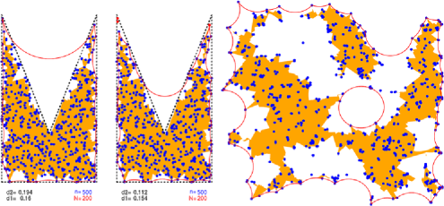
The first example (left-hand and central panel of Figure 4) illustrates the estimation (from $n=500$ uniform points) of the $\pi/4$-cone convex set $S=[0,1]\times[0,t+1/2]\setminus T$ where $t=\frac{1}{2}\tan(3\pi/8)$, $T$ being the isosceles triangle with vertices $(0,t+1/2)$, $(1,t+1/2)$, $(1/2,1/2)$. For the ccc-hull (the shaded area in the figures), we have used $\rho=\pi/4$ and $h=1/2$ with $N=200$ cones. For the $r$-convex hull (whose boundary is marked in continuous lines as a union of $r$-circumference arcs), we took $r=1/2$ (left-hand panel) and $r=1/4$ (central panel). The whole point of choosing this set is to show that, even in very simple cases, the presence of an inward nonsmooth peak can lead to a situation for which the $r$-convex hull provides an “oversmoothed” estimation since the estimator just cannot “go inside” the sharp “gulf” in the set. This is not the case of the ccc-hull which is designed to deal with such unsmooth situations. Of course, we might improve things by choosing a smaller value of $r$ but, in any case, the $r$-convex is inconsistent for any $r$ and, at the end, it will we outperformed by the $\rho,h$-ccc hull, provided that a suitable value of $\rho$ ($\leq\pi/4$ in this case) is chosen.

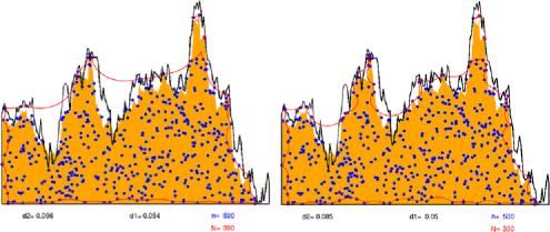
The second example (right-hand panel of Figure 4) shows the behavior of our estimator (with $\rho=\pi/3$, $h=1/8$) when compared with the $r$-convex hull (the circumference arcs in continuous lines) with $r=1/10$ for a sample of points that represent the locations $(x,y)$ of bramble canes in a field of 9 square meters, rescaled to the unit square. This data set can be found in the R-library spatstat; see hut79 and dig83 for further details; we have ignored the labels identifying different classes of plants, according to their ages. Of course, in this example there is no “true” set to give an objective comparison. We can see, however, how both estimators give a quite different estimation of the “habitat” of these plants and the ccc-hull seems better adapted to detect the absence of canes in some areas. Finally, the third example shows the estimation of a quite irregular set: the hypograph of the trajectory of a Brownian motion on the unit interval. We define the hypograph of a positive function $f$ defined on $[a,b]$ by $H(f)=\{(x,y)\dvtx x\in[a,b],0\leq y\leq f(x)\}$. In our example, the Brownian trajectory has been shifted vertically in order to take all values above zero. The estimation of hypographs is a major aim in the problem of efficient boundary, a relevant topic in econometrics; see, for example, Simar and Wilson sim00 . An additional interest of this example is to show how our ccc-hull can be adapted to incorporate the information that our target set is an hypograph; this can be made by just choosing vertical cones and restricting their rotation angle in the algorithm. In this case, we have taken $n=500$, $\rho=\pi/6$, $h=1$, with $N=300$ cones but the rotation angles in the algorithm have been restricted between $5\pi/12$ and $7\pi/12$ in order the keep the structure of an hypograph; see Figure 5. The parameters for the $r$-convex estimator are $r=1/8$ (left panel in Figure 5), and $1/16$ (right panel); note that there is no way to adapt the $r$-convex hull to the hypograph shape. In this case, the ccc-hull, with the hypograph information incorporated, clearly outperforms the $r$-convex hull.

Figure 5: Hypograph of a trajectory of a Brownian motion: the shaded area is the ccc-hull; continuous lines made of $r$-arcs correspond to the boundaries of the $r$-convex hull for $r=1/8$ (left) and $r=1/16$ (right).

7.2 Simulation outputs

We have carried out a small simulation study to compare the performance of the ccc-hull with that of the $r$-convex hull for different sample sizes and values of the parameters. The target set $S_{1}=[0,1]^{2}\setminus\bigcup_{i=1}^{4}T_{i}$ where the $T_{i}$ are triangles with vertices $(0,1)$, $(1/2,1/2)$, $(1,1)$; $(0,0)$, $(1/2,1/2)$, $(1,0)$; $(0,1/3)$, $(1/2,1/2)$, $(0,2/3)$ and $(1,1/3)$,$(1/2,1/2)$, $(1,2/3)$. This set is $\rho_{0}=2\arctan(1/3)$-cone convex. Figure 6 corresponds to the case $\rho=\pi/5$, $h=1/2$, $N=1000$ and $r=1/6$ for the $r$-convex hull with $n=1200$ uniform points.

Figure 6: Ccc-hull (shaded area) and $r$-convex hull (boundary made of $r$-arcs) constructed from 1200 points of $S_{1}$. Here, $\rho=\pi/5$, $h=1/2$, $r=1/6$.

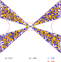
Table 1 shows the expected values, over 500 runs (and their standard deviations in parenthesis) for the errors in measure [$d_{1}=d_{\mu}(S,{\mathbb{C}}_{\rho,h}(\aleph_{n}))$, $d_{2}=d_{\mu}(S,C_{r}(\aleph_{n}))$] of both estimators (the ccc-hull and the $r$-convex hull), with different values of the parameters $\rho$, $r$ and $h$. For small sample sizes (200 in Table 1) the $r$-convex hull has a smaller error in measure. However, as the sample size increases, (from 400 on the ccc-hull outperforms the $r$-convex hull. We have taken $N=200$ cones for the simulation, and the distances were calculated by the Monte Carlo method using 4000 uniform random observations.

Table 1: Average errors (and standard deviations) over 500 runs for the ccc-hull ($d_{1}$) and the $r$-convex hull ($d_{2}$) in the estimation of $S_{1}$

	$\bolds{d_{1}}$	$\bolds{d_{2}}$	$\bolds{d_{1}}$	$\bolds{d_{2}}$
$\bolds{n}$	$\bolds{\rho=\rho_{0},h=1/3}$	$\bolds{r=1/4}$	$\bolds{\rho=\pi/5,h=1/2}$	$\bolds{r=1/6}$
200	0.204 (0.011)	0.191 (0.009)	0.197 (0.011)	0.161 (0.010)
400	0.138 (0.009)	0.180 (0.008)	0.134 (0.010)	0.140 (0.008)
600	0.107 (0.008)	0.174 (0.007)	0.105 (0.008)	0.132 (0.007)
800	0.090 (0.007)	0.172 (0.007)	0.089 (0.007)	0.127 (0.007)
1000	0.080 (0.007)	0.170 (0.007)	0.078 (0.007)	0.124 (0.006)
1200	0.070 (0.006)	0.169 (0.006)	0.070 (0.006)	0.122 (0.006)

8 Final remarks: Some suggestions for further work

In our view, the study of the following topics might be of interest in connection with the notion of cone-convexity introduced in this paper.

Applications to home-range estimation. As commented above, our cone-convex hulls are in fact a considerable generalization of the simpler classical notion of convex-hull. Such generalizations (the $r$-convex hull is another example of them) are relevant in those application fields where more flexible set estimators are needed. An example arises in zoology and ecology, in the problem of home range estimation. A commonly cited definition of animal’s home range is that of Burt bur43 : “that area traversed by the individual in its normal activities of food gathering, mating and caring for young.” The problem of estimating the home range from “sightings” or GPS records of animal positions has received a considerable attention (see, e.g., Anderson and82 for an introduction). As pointed out by Burgman and Fox bur03 , “Minimum convex polygons (convex hulls) are an internationally accepted, standard method for estimating species’ ranges, particularly in circumstances in which presence-only data are the only kind of spatially explicit data available”. These authors also discuss the obvious drawbacks of the convex hull, and analyze in some detail the so called $\alpha$-hulls (conceptually related with the $r$-convex hulls discussed above) as a useful more flexible alternative. In fact, the idea of considering different nonparametric estimators in home range estimation is far from new. Many highly cited papers (Worton wor89 , Getz and Wilmers get04 , etc.) have considered this topic. Some of them, in particular, Worton wor89 , analyze the use of auxiliary density estimators to construct home range estimators. We believe that our proposal here, based on the cone-convex hull, could be seen as a further step in this advance toward flexibility and generality from the classical approach based on the “hull principle.” The reason is that our estimator could be suitable for those problems where highly irregular shapes, including central holes of sharp inward peaks, are to be expected, due to existence of geographic obstacles leading to irregular habitats. For example, Getz and Wilmers get04 have suggested (in a nonmathematical journal) an interesting class of estimators based on the union of convex hulls of the nearest neighbours of every sample point. These authors convincingly motivate their proposal on the basis of detailed examples. Again, the point is the need of flexible, general estimators for home range studies and related problems. However, to the best of our knowledge, the theoretical properties of that class of estimators have not been analyzed so far. In a way, our proposal in this paper, aims at same goals having still in mind the idea of extending the classical convex hull. While the detailed analysis of such practical applications is beyond the scope of this paper, we hope that the real-data example (not in zoology but in botany) outlined in the previous section could give a hint on the possible advantages of our estimators.

Inference on the parameter $\rho$. In our cone-convexity definitions, the parameter $\rho$ has an obvious intuitive interpretation (in terms of the sharpest inward peak in the domain), even more direct than that of the parameter $r$ in the $r$-convexity property. So, given a domain $S$, the inference on the largest value of $\rho$ fulfilling the cone-convexity property (for a given $h$) might be of some interest from the image analysis point of view. In particular, the study of a suitable test for the hypothesis $H_{0}\dvtx\rho\geq\rho_{0}$ seems a natural aim. Note that in the case $\rho_{0}=\pi$ this would essentially amount to test convexity. The theory of multivariate spacings, as developed, for example, by Janson jan87 , seems to be a relevant auxiliary tool in this problem.

Cone-convexity for functions. Our cone-convexity concepts have been primarily defined for sets but they could be extended in a natural way for real functions $f\dvtx[a,b]^{d}\rightarrow{\mathbb{R}}$: we could say that $f$ is $\rho$-cone-convex when the hypograph $H(f)=\{(x,y)\dvtx x\in[a,b]^{d},y\leq f(x)\}$ is $\rho$-cone-convex. The distance between two $\rho$-cc functions might then be defined in terms of the Hausdorff distance between the corresponding hypographs; similar ideas have been considered elsewhere, for example, Sendov sen90 . On the one hand, this Hausdorff-based metric would provide a “visual” proximity criterion (potentially meaningful in many real-world applications) between the data. On the other hand, the cone-convexity assumption would lead to a natural way for data smoothing. For example, in the setting of a nonparametric regression model $y_{i}=f(x_{i})+\varepsilon_{i}$ (with $d=1$), we could think of recovering the function $f$ from the data $(x_{i},y_{i})$ under the assumption that $f$ is $\rho$-cone-convex. Other applications to Functional Data Analysis (in particular to supervised functional classification) are also under study.

Appendix

Proof of Proposition 3 Let $C$ be a member of the class $\Lambda_{\rho,h}(x)$. Without loss of generality, take $C=C_{\rho,e_{1},h}(0)$ where $e_{1}$ is the first vector in the canonical basis. The reasoning for any other cone $C=C_{\rho,\xi,h}(z)$ is reduced to this case by translation and/or rotation.

Figure 7: Case 3, $C_{\gamma,\nu,h_{1}}(x)\subset C_{\rho,e_{1},h}(0)$.

By definition of the class, we have $x\in C_{\rho,e_{1},h}(0)$. As a first step in the proof, it will be useful to consider three possible situations regarding the position of $x$. In all three cases, we will be able to find a cone $C^{\prime}=C_{\gamma,v,h_{1}}(x)\subset C$.

[1.]

If $x\in C_{\rho,e_{1},h/2}(0)$, then $C^{\prime}\subset C_{\rho,e_{1},h}(0)$ for $C^{\prime}=C_{\gamma,e_{1},h_{1}}(x)$.

If $x=re_{1}$ with $h/2\leq r<h$, then $C^{\prime}\subset C_{\rho,e_{1},h}(0)$ for $C^{\prime}=C_{\gamma,-e_{1},h_{1}}(x)$ since $h_{1}$ is smaller than the distance from $he_{1}/2$, the middle point of the axis of $C=C_{\rho,e_{1},h}(0)$, to the boundary of $C$.

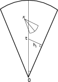
For any other $x\in C_{\rho,e_{1},h}(0)$, note that $t=he_{1}/2$ corresponds to the least favorable position of the vertex of a $\gamma,h_{1}$-cone, $C^{\prime}$ in order to get $C^{\prime}\subset C$. Let $\lambda_{1}$ be the solution of $\langle\frac{\lambda_{1}t-x}{\|\lambda_{1}t-x\|},\frac{-x}{\|x\|}\rangle=\cos(\gamma/2)$. Then if we take a cone $C^{\prime}=C_{\gamma,v,h_{1}}(x)$ with axis $v=\frac{\lambda_{1}t-x}{\|\lambda_{1}t-x\|}$ we also get $C^{\prime}\subset C_{\rho,e_{1},h}(0)$; see Figure 7.

Finally, the unavoidable family is constructed by selecting a finite number of directions $\xi_{j}$ such that the cones $\{\overline{C_{\gamma/2,\xi_{j},h_{1}}(x)}\}_{j=1,\ldots,k}$ are a minimal covering of $\overline{B(x,h_{1})}$. Indeed, given $C\in{\Lambda}_{\rho,h}(x)$ the point $x\in C$ is in one of the three previously considered cases so that there exists a unit vector $\xi$ for which $C_{\gamma,\xi,h_{1}}(x)\subset C$. Since $\{\overline{C_{\gamma/2,\xi_{j},h_{1}}(x)}\}_{j=1,\ldots,k}$ is a covering of $\overline{B(x,h_{1})}$, we can take $j_{0}$ such that $\langle\xi_{j_{0}},\xi\rangle\geq\gamma/2$. Therefore, $C_{\gamma/2,\xi_{j_{0}},h_{1}}(x)\subset C_{\gamma,\xi,h_{1}}(x)$. The final statement about the cardinality follows directly from the construction.

Proof of Theorem 7 Note that $F$ is a volume function (and hence a Kneser function) as those considered in Stachó sta76 . According to Lemma 2 in that paper, $F$ is absolutely continuous and $F^{\prime}(t)$ exists except for a countable set. So, there exist a countable set $N$ and positive constants $s$ and $q$ such that $F^{\prime}(t)<q$ $\forall t\in[0,s]\cap N^{c}$. If we take $h_{2}=\min\{s,h_{1}\}$, where $h_{1}=\frac{h}{2}\sin(\rho/2)$, then according with equation (5.2):

$$\mathbb{E}\bigl{(}d_{P_{X}}\bigl{(}S,\tilde{\mathbb{C}}_{\rho,h}(\aleph_{n})\bigr{)}\bigr{)} \leq k_{2}\int_{\{x\in S:d(x,\partial S)\leq h_{2}\}}\sum_{U\in\mathfrak{U}_{x,\rho,h}}\bigl{(}1-k_{1}\mu(U\cap S)\bigr{)}^{n}\,dx$$

$${}+k_{2}\int_{\{x\in S:d(x,\partial S)>h_{2}\}}\sum_{U\in\mathfrak{U}_{x,\rho,h}}\bigl{(}1-k_{1}\mu(U\cap S)\bigr{)}^{n}\,dx.$$

With respect to the last term, note that $d(x,\partial S)>h_{2}$ entails $B(x,h_{2})\subset S$ and for all $U\in\mathfrak{U}_{x,\rho,h}$, we have: $k_{1}\mu(U\cap S)\geq k_{1}\mu(U\cap B(x,h_{2}))=c_{0}h_{2}^{d}$ for some positive $c_{0}$. Therefore, if $k=k(\rho,h)$ denotes the cardinality of the set $\mathfrak{U}_{x,\rho,h}$ then

$$\int_{\{x\in S:d(x,\partial S)>h_{2}\}}\sum_{U\in\mathfrak{U}_{x,\rho,h}}\bigl{(}1-k_{1}\mu(U\cap S)\bigr{)}^{n}\,dx$$

$$\qquad\leq k\bigl{(}1-c_{0}h_{2}^{d}\bigr{)}^{n}\mu\bigl{(}\bigl{\{}x\in S\dvtx d(x,\partial S)>h_{2}\bigr{\}}\bigr{)},$$

which can be upper bounded by $k_{3}e^{-nh_{2}^{d}c_{0}}$, for some positive constant $k_{3}$.

In order to bound the first integral, note that if $U=C_{\gamma/2,\xi_{j},h_{1}}(x)$ and $t\leq h_{2}\leq h_{1}$ then $U\cap B(x,t)=C_{\gamma/2,\xi_{j},t}(x)$ and so, if $d(x,\partial S)=t$

$$k_{1}\mu(U\cap S)\geq k_{1}\mu\bigl{(}U\cap B(x,t)\bigr{)}=c_{0}t^{d}.$$

Therefore,

$$\int_{\{x\in S:d(x,\partial S)\leq h_{2}\}}\sum_{U\in\mathfrak{U}_{x,\rho,h}}\bigl{(}1-k_{1}\mu(U\cap S)\bigr{)}^{n}\,dx$$

$$\qquad\leq\int_{\{x\in S:d(x,\partial S)\leq h_{2}\}}k\bigl{(}1-c_{0}d(x,\partial S)^{d}\bigr{)}^{n}\,dx$$

$$\qquad\leq\int_{\{x\in S:d(x,\partial S)\leq h_{2}\}}ke^{-c_{0}nd(x,\partial S)^{d}}\,dx.$$

Next, let $g(z)=ke^{-c_{0}nz^{d}}$. A change of variables leads to

$$\int_{\{x\in S:d(x,\partial S)\leq h_{2}\}}ke^{-c_{0}nd(x,\partial S)^{d}}\,dx = \int_{\{x\in S:d(x,\partial S)\leq h_{2}\}}g\bigl{(}d(x,\partial S)\bigr{)}\,dx$$

$$= \int_{[0,h_{2}]}g(z)\,dF(z)$$

$$= \int_{[0,h_{2}]}g(z)F^{\prime}(z)\,dz\leq\int_{[0,h_{2}]}k_{4}e^{-c_{0}nz^{d}}\,dz,$$

with $k_{4}$ a positive constant (we have used in the last inequality the essential boundedness $F^{\prime}$ in $[0,s]$). Finally, we have that there exists $k_{5}>0$ such that

$$\int_{[0,h_{2}]}k_{4}e^{-c_{0}nz^{d}}\,dz = n^{-1/d}\int_{0}^{c_{0}nh_{2}^{d}}k_{5}e^{-u}u^{(1-d)/d}\,du$$

$$\leq n^{-1/d}\int_{0}^{+\infty}k_{5}e^{-u}u^{(1-d)/d}\,du$$

$$= \mathcal{O}\bigl{(}n^{-1/d}\bigr{)}.$$

Collecting bounds, we get $\mathbb{E}(d_{P_{X}}(S,\tilde{\mathbb{C}}_{\rho,h}(\aleph_{n})))=\mathcal{O}(e^{-nh_{2}^{d}c_{0}}+n^{-1/d})=\mathcal{O}(n^{-1/d})$.