Quantum phase transitions in exactly solvable one-dimensional compass models

Abstract

We present an exact solution for a class of one-dimensional compass models which stand for interacting orbital degrees of freedom in a Mott insulator. By employing the Jordan-Wigner transformation we map these models on noninteracting fermions and discuss how spin correlations, high degeneracy of the ground state, and $Z_{2}$ symmetry in the quantum compass model are visible in the fermionic language. Considering a zigzag chain of ions with singly occupied $e_{g}$ orbitals ($e_{g}$ orbital model) we demonstrate that the orbital excitations change qualitatively with increasing transverse field, and that the excitation gap closes at the quantum phase transition to a polarized state. This phase transition disappears in the quantum compass model with maximally frustrated orbital interactions which resembles the Kitaev model. Here we find that finite transverse field destabilizes the orbital-liquid ground state with macroscopic degeneracy, and leads to peculiar behavior of the specific heat and orbital susceptibility at finite temperature. We show that the entropy and the cooling rate at finite temperature exhibit quite different behavior near the critical point for these two models.

I Introduction

In recent years the growing interest in orbital degrees of freedom for strongly correlated electrons in transition-metal oxides (TMOs) Kug82 ; Fei97 ; Tokura ; Hfm , was amplified by complex phenomena uncovered in theory and experiment, such as the interplay between spin and orbital degrees of freedom Ole05 ; Kha05 ; Ole12 , consequences of orbital degeneracy in the perovskite vanadates Hor03 , phase transitions to magnetic and orbital order Hor08 , dimerization in ferromagnetic spin-orbital chains Her11 , entanglement entropy spectra in one-dimensional (1D) models,You12 , and exotic types of spin order triggered by spin-orbital entanglement in the Kugel-Khomskii models Brz13 . Electrons are strongly correlated and localize due to large on-site Coulomb interaction $U$ — then they interact by superexchange. While spin and orbital degrees of freedom are generally entangled and influence each other on superexchange bonds Ole12 ; You12 ; Brz14 , or due to local spin-orbit coupling Jac09 ; Cha10 . In spin-orbital systems an electron can break into a spinon and an orbiton Woh11 , as observed recently in Sr₂CuO₃ Sch12 . This motivates a more careful study of orbital models in low dimension. Such models for Mott insulators, depend on the type of partly filled $3d$ orbitals, with either $e_{g}$ symmetry vdB99 ; vdB04 ; Fei05 ; Ryn10 , or $t_{2g}$ symmetry Dag08 ; Wro10 ; Tro13 ; Che13 .

In TMOs with the perovskite structure active orbitals are selected by the octahedral crystal field due to the oxygen ions which splits the $3d$ quintet at a transition-metal ion into a $t_{2g}$ triplet and an $e_{g}$ doublet at higher energy. Well known examples of $e_{g}$ systems with partly filled $e_{g}$ orbitals by one spin flavor which are of interest here are: (i) $d^{4}$ ions (in LaMnO₃, Rb₂CrCl₄, or KCrF₃) Fei99 , (ii) $d^{7}$ ions in LiNiO₂ Rei05 , or (iii) $d^{9}$ ions Kug82 in KCuF₃, K₃Cu₂F₇, or K₂CuF₄ Brz13 . In all these systems the $t_{2g}$ orbitals are either completely filled (in the $d^{7}$ and $d^{9}$ configurations), or contain one electron each (in the $d^{4}$ configuration) – in the latter case their spins are aligned with the spin of an $e_{g}$ electron due to Hund’s exchange. The two $e_{g}$ orbitals represent then the dynamical degrees of freedom.

Here we focus on ferromagnetic states with spins fully polarized were only the orbital degrees of freedom being active. Orbitals are interacting via generically anisotropic superexchange interactions $\propto J_{\gamma}$ depending on the bond direction $\gamma=a,b$. Thus a typical orbital superexchange model has the following anisotropic form,

$$H_{J}=\sum_{\langle ij\rangle\parallel\gamma}J_{\gamma}T_{i}^{\gamma}T_{j}^{\gamma}.$$ (1)

This model stands for intrinsically frustrated directional orbital interactions on the square lattice, and may represent both $e_{g}$ vdB99 and $t_{2g}$ orbital interactions Dag08 . In the latter case the operators include just one of the orthogonal pseudospin components at each bond and are Ising-like. This form of interactions is found as well in the compass models vdB13 ; Nus05 ; Dou05 ; Dor05 ; Chen07 ; Wen08 ; Orus09 ; Cin10 ; Brz10 ; Tro10 ; Brz07 ; Brz09 , and in the Kitaev model on the honeycomb lattice Kit06 ; Che08 ; Div09 .

The interactions that are considered here are defined by the pseudospin operators $T^{\gamma}_{i}$ for two active orbitals (for $T=1/2$), and we define them as linear combinations of the Pauli matrices $\{\sigma_{i}^{x},\sigma_{i}^{y}\}$ representing the two pseudospin components on odd/even bonds notesz ,

$$\tilde{\sigma}_{i}(\pm\theta)\equiv\cos(\pm\theta/2)\,\sigma_{i}^{x}+\sin(\pm\theta/2)\,\sigma_{i}^{y}.$$ (2)

These operators define the generalized compass model (GCM) considered in this paper. In the 1D GCM the interactions depend on the $x$-th and $y$-th orbital component in Eq. (2), but the exchange interactions are bond dependent as in Eq. (1) and alternate between even ($J_{\rm e}$) and odd ($J_{\rm o}$) exchange bonds along the 1D chain of $N$ sites (we consider periodic boundary conditions, and even values of $N$),

$$H_{J}(\theta)=\sum_{i=1}^{N/2}\left\{J_{\rm o}\tilde{\sigma}_{2i-1}(\theta)\tilde{\sigma}_{2i}(\theta)+J_{\rm e}\tilde{\sigma}_{2i}(-\theta)\tilde{\sigma}_{2i+1}(-\theta)\right\},$$ (3)

where we sum over unit cells. For a representative pseudospin $\tilde{\sigma}_{i}$ the interaction involves the quantization axis with direction $\theta$ for one bond and the one with $-\theta$ for the other, so each pseudospin has to find some compromise. This frustration increases gradually with increasing angle $\theta$ when the model Eq. (3) interpolates between the Ising model at $\theta=0$ to the quantum compass model (QCM) at $\theta=\pi/2$ Cin10 . The latter is also called the 1D Kitaev model by some authors Div09 . In the intermediate case, $\theta=\pi/3$, one finds orbital superexchange (1) for the $e_{g}$ orbital model (EOM) or $60^{\circ}$ compass model (for the angle $\theta=\pi/3$).

The EOM (at $\theta=60^{\circ}$) was first introduced as an effective model for perovskite $e_{g}$ orbital systems vdB99 , and next considered in two-dimensional (2D) and three-dimensional (3D) ferromagnetic TMOs with active $e_{g}$ orbitals Ole05 ; vdB99 ; Nus04 ; Bis05 . The equivalent planar model describes the insulating phase of $p$-band fermions in triangular, honeycomb and kagome optical lattices Zhao08 ; Wu08 .

The QCM arises from the GCM Eq. (3) with frustrated Ising-like interactions tuned by an angle $\theta$ on a square lattice Cin10 at $\theta=90^{\circ}$. While 2D Ising models with frustrated interactions have long-range order at finite temperature Lon80 , one might expect that disordered states emerge when interacting spin components depend on the bond direction, as in Eq. (1). This is indeed the case of the Kitaev model on a hexagonal lattice with a spin-liquid ground state that is exactly solvable Kit06 . Instead, the infinite degeneracy in the ground state for the classical compass model on 2D or 3D cubic lattices is lifted via the order-out-of-disorder mechanism and a directional ordering of fluctuations appears at low temperature Mis04 . For the quantum version, it has been rigorously proven in terms of the reflection positivity method You07 that the alternating orbital order is stable in the 2D planar $60^{\circ}$ compass model at zero temperature. Indeed, this result is confirmed by numerical simulations Wen08 .

The QCM is characterized by an exotic property of the dimensional reduction which implies that a $d$-dimensional system has long-range order in $(d-1)$ dimension vdB13 ; You08 . For example, the global ground states of the 2D QCM have a ferro-orbital nematic long-range order in a highly degenerate ground state Brz10 ; You10 ; He11 . It has been shown that this directional long-range order survives in a manifold of low energy excited states when the compass interactions are perturbed by the Heisenberg ones Tro10 — this property opens its potential application in quantum computation. It is remarkable that the 2D QCM is dual to the toric code model in transverse magnetic field Vid09 and to the Xu-Moore model (Josephson arrays) Xu04 .

Quantum phase transitions (QPTs) between different types of order were established in the 1D QCM Brz07 , in a quantum compass ladder Brz09 , and in the 2D QCM Nus05 ; Dou05 ; Dor05 ; Chen07 ; Wen08 ; Orus09 ; Cin10 ; Brz10 ; Tro10 , when anisotropic interactions are varied through the isotropic point and the ground state switches between two different types of Ising nematic order dictated by either interaction. At the transition point itself, i.e., when the competing interactions are balanced, the ground state is highly degenerate and contains states which correspond to both relevant kinds of nematic order. The correlations along perpendicular direction to that of the nematic order are restricted to nearest neighbor (NN) sites You11 , and certain NN spin correlations change discontinuously at the critical point. Studies of the 1D QCM using entanglement measures and quantum discord in the ground state show that the correlations between two orbitals on some bonds are essentially classical You12b . The QPT driven by the transverse field emerges only at zero field and is of the second order Sun09 .

The purpose of this paper is to present an exact solution of the GCMs (with orbitals of $e_{g}$ or $t_{2g}$ symmetry), and to investigate their properties at finite temperature. We propose a possible scenario provided by a 1D zigzag lattice which can be prepared in layered structures of TMOs Xiao11 , or are realized in optical lattices by fermions occupying $p_{x}$ and $p_{y}$ orbitals Simon11 ; Gsun . Our motivation is twofold: On one hand, recently artificial heterostructures of TMOs are becoming available, and the modern technologies and allow to devise artificial 1D quantum systems, such as quantum wires or rings. In terms of interface engineering, some models can be designed, such as a 2D design for man-made honeycomb lattice Xiao11 . On the other hand, the zigzag chain of $S=1/2$ spins, with active $xy$ and $yz$ orbitals in $d^{1}$ states at Ti³⁺ ions, is found in pyroxene titanium oxides ATiSi₂O₆ (A = Na,Li) Kon04 ; Hik04 . The alternation of the Ti-Ti distance is a direct consequence of orbital dimerization. We also solve exactly the GCM at arbitrary angle $\theta$ and compare its properties with those of the EOM. We find that the EOM and the 1D QCM are both characterized by a QPT, but we uncover an important difference between these transitions which is found for the anisotropic interactions.

The paper is organized as follows: We introduce the EOM in Sec. II.1 and present its exact solution in Sec. II.2 obtained using the Jordan-Wigner transformation. We show that a gap found in the excitation spectrum persists also in the entire range of angle $\theta$ in the GCM, see Sec. III.1. Properties of the GCM, including the dependence of transverse orbital polarization and intersite pseudospin correlations on the angle $\theta$ and on the polarizing field are investigated in Sec. III.2. This field is responsible for the switch of the pseudospin order at the QPT. Next we present exact results at finite temperature obtained for the entropy and for the orbital cooling rate in Sec. IV.1, and for the specific heat in Sec. IV.2. The orbital polarization induced by finite field and orbital susceptibility are analyzed in Sec. IV.3. The paper is concluded with a final discussion and summary in Sec. V. Here we also highlight the interpretation of the results in terms of fermionic bands as equivalent to the spin correlations. These correlations follow from the $Z_{2}$ symmetry, as explained in the Appendix.

II Orbital compass model

II.1 One-dimensional zigzag $e_{g}$ orbital model

We consider first the exact solution for the 1D EOM (60^∘ compass model) of Fig. 1, with the Hamiltonian $H_{J}$ given by Eq. (38) at $\theta=\pi/3$. This example serves as a general guideline for the analytic solution and for the thermodynamics presented below in Secs. III-IV. The interactions in Eq. (1) are given by operators

$$T_{i}^{a(b)}=-\frac{1}{2}\sigma_{i}^{y}\pm\frac{\sqrt{3}}{2}\sigma_{i}^{x},$$ (4)

which depend on Pauli matrices, $\{\sigma_{i}^{\alpha}\}$ ($\alpha=x,y$) for $e_{g}$ orbital states notesz . In the case of a 3D cubic system Eq. (4) would be augmented by $T_{i}^{c}=\sigma_{i}^{y}$ for the bonds along the $c$ axis. The interactions follow from the Kugel-Khomskii superexchange Kug82 ; Fei97 , as well as from Jahn-Teller distortions Zaa93 . Typically both these terms contribute jointly to the orbital exchange interactions $J_{\gamma}$ in Eq. (1), as in LaMnO₃ Fei99 . Another example is the phonon-mediated orbital exchange in spinels Rad05 which has the form of interaction with an effective exchange $J_{\gamma}=g^{2}/k_{F_{1g}}$, where $g$ is a Jahn-Teller coupling constant and $k_{F_{1g}}$ is the elastic constant of $F_{1g}$ phonons.

Figure 1: (Color online) Zigzag chain in an $(a,b)$ plane with one hole (or electron) per site in $e_{g}$ states of a Mott insulator. The directional orbitals, $3x^{2}-r^{2}$ and $3y^{2}-r^{2}$, are the most convenient choice to calculate the orbital superexchange interactions along the $a$ and $b$ cubic axis, respectively. In the usual $e_{g}$ orthogonal orbital basis $\{3z^{2}-r^{2},x^{2}-y^{2}\}$ such interactions may cause orbital flips as the orbital flavor is not conserved in intersite hopping processes (charge excitations) vdB99 . If two $t_{2g}$ orbitals, $zx$ and $yz$, are considered instead, only diagonal hopping between pairs of these orbitals occurs along the bonds parallel to the $a$ or $b$ axis Dag08 , and one finds the 1D quantum compass model Brz07 .

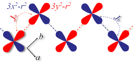
For the zigzag chain of $N$ sites (assumed here to be even, and $N^{\prime}=N/2$ is the number of two-site unit cells) shown in Fig. 1, the interactions with exchange constants $J_{\rm e}$ and $J_{\rm o}$ alternate between even and odd bonds, as in Eq. (3),

$${\cal H}_{e_{g}} \!=\! H_{J}+H_{h}$$ (5)

$$\!=\! \sum_{i=1}^{N/2}\left\{J_{\rm o}\left(\frac{\sqrt{3}}{2}\sigma_{2i-1}^{x}+\frac{1}{2}\sigma_{2i-1}^{y}\right)\!\left(\frac{\sqrt{3}}{2}\sigma_{2i}^{x}+\frac{1}{2}\sigma_{2i}^{y}\right)\right.$$

$$+\left.J_{\rm e}\left(\frac{\sqrt{3}}{2}\sigma_{2i}^{x}-\frac{1}{2}\sigma_{2i}^{y}\right)\!\left(\frac{\sqrt{3}}{2}\sigma_{2i+1}^{x}-\frac{1}{2}\sigma_{2i+1}^{y}\right)\right\}$$

$$+ \frac{h}{2}\;\sum_{i}\left(\sigma_{2i-1}^{z}+\sigma_{2i}^{z}\right).$$

The model Eq. (5) includes a crystal field term,

$$H_{h}=\frac{h}{2}\;\sum_{i}\left(\sigma_{2i-1}^{z}+\sigma_{2i}^{z}\right),$$ (6)

which is the source of the orbital polarization field $h$ along the $z$-th pseudospin component. It follows from the uniform expansion or compression of the lattice along the $c$ axis, i.e., orthogonal to the $ab$ plane of the chain. Although we consider for clarity $J_{\rm o}>0$ and $J_{\rm e}>0$ below, the model is invariant with respect to the gauge transformation changing signs of both couplings $\{J_{\rm o},J_{\rm e}\}$ simultaneously, as alternating orbital and ferro-orbital systems are related to one another. This can be realized explicitly by introducing the operator ${\cal U}=\Pi_{i}\sigma^{z}_{2i-1}$.

The Hamiltonian (5) can be exactly diagonalized following the standard procedure for 1D systems. The Jordan-Wigner transformation maps explicitly between pseudospin operators and spinless fermion operators by

$$\sigma_{j}^{+} = \exp\left[i\pi\sum_{i=1}^{j-1}c_{i}^{\dagger}c_{i}\right]c_{j}=\prod_{i=1}^{j-1}\sigma_{i}^{z}c_{j},$$ (7)

$$\sigma_{j}^{-} = \exp\left[-i\pi\sum_{i=1}^{j-1}c_{i}^{\dagger}c_{i}\right]c_{j}^{\dagger}=\prod_{i=1}^{j-1}\sigma_{i}^{z}c_{j}^{\dagger},$$ (8)

$$\sigma_{j}^{z} = 1-2c_{j}^{\dagger}c_{j}.$$ (9)

Next discrete Fourier transformation for odd/even spin sites is introduced as follows ($j=1,\dots,N^{\prime}$),

$$c_{2j-1} = \frac{1}{\sqrt{N^{\prime}}}\sum_{k}e^{-ikj}a_{k},$$ (10)

$$c_{2j} = \frac{1}{\sqrt{N^{\prime}}}\sum_{k}e^{-ikj}b_{k},$$ (11)

with the discrete momenta $k$ which correspond to the reduced Brillouin zone and are given by

$$k=\frac{n\pi}{N^{\prime}},\quad n=-(N^{\prime}-1),-(N^{\prime}-3),\ldots,(N^{\prime}-1).$$ (12)

The Hamiltonian (5) in the momentum representation becomes a quadratic form, with mixed $k$ and $-k$ fermionic states,

$${\cal H}_{e_{g}} = \sum_{k}\left[B_{k}a_{k}^{\dagger}b_{-k}^{\dagger}+A_{k}a_{k}^{\dagger}b_{k}+A_{k}^{*}b_{k}^{\dagger}a_{k}+B_{k}^{*}b_{-k}a_{k}\right]$$ (13)

$$+ h\sum_{k}(a_{k}^{\dagger}a_{k}+b_{k}^{\dagger}b_{k})-hN^{\prime},$$

where

$$A_{k} = J_{\rm o}+J_{\rm e}e^{ik},$$ (14)

$$B_{k} = J_{\rm o}e^{i\pi/3}-J_{\rm e}e^{i(k-\pi/3)}.$$ (15)

The present Hamiltonian may be easily diagonalized by a Bogoliubov transformation, as shown below.

II.2 Exact solution and energy spectrum

To diagonalize the Hamiltonian Eq. (13), we first rewrite it in the symmetrized matrix form with respect to the $k\leftrightarrow-k$ transformation,

$${\cal H}_{e_{g}}=\frac{1}{2}\sum_{k}\;(a_{k}^{\dagger},a_{-k},b_{k}^{\dagger},b_{-k})\left(\begin{array}[]{cccc}h&0&A_{k}&-(P_{k}+Q_{k})\\ 0&-h&-(P_{k}-Q_{k})&-A_{k}\\ A_{k}^{*}&-(P_{k}^{*}-Q_{k}^{*})&h&0\\ -(P_{k}^{*}+Q_{k}^{*})&-A_{k}^{*}&0&-h\end{array}\right)\!\left(\begin{array}[]{c}a_{k}\\ a_{-k}^{\dagger}\\ b_{k}\\ b_{-k}^{\dagger}\end{array}\right),$$ (16)

where we have introduced

$$P_{k} \equiv \cos\frac{\pi}{3}\,(J_{\rm e}e^{ik}-J_{\rm o}),$$ (17)

$$Q_{k} \equiv -i\sin\frac{\pi}{3}\,(J_{\rm e}e^{ik}+J_{\rm o}).$$ (18)

Eq. (16) is now diagonalized by a $(4\times 4)$ Bogoliubov transformation which connects original $\{a_{k}^{\dagger},a_{-k}^{\dagger},b_{k}^{\dagger},b_{-k}^{\dagger}\}$ fermions with new $\{\alpha_{k}^{\dagger},\alpha_{-k}^{\dagger},\beta_{k}^{\dagger},\beta_{-k}^{\dagger}\}$ quasiparticle (QP) operators,

$$\left(\begin{array}[]{c}\alpha_{k}^{\dagger}\\ \alpha_{-k}\\ \beta_{k}^{\dagger}\\ \beta_{-k}\end{array}\right)=\hat{U}_{k}\left(\begin{array}[]{c}a_{k}^{\dagger}\\ a_{-k}\\ b_{k}^{\dagger}\\ b_{-k}\end{array}\right),$$ (27)

where the rows of the $4\times 4$ matrix $\hat{U}_{k}$ are eigenvectors following from:

$$\left[{\cal H}_{e_{g}},\alpha_{k}^{\dagger}\right] = \varepsilon_{k,1}\alpha_{k}^{\dagger},$$ (28)

$$\left[{\cal H}_{e_{g}},\beta_{k}^{\dagger}\right] = \varepsilon_{k,2}\beta_{k}^{\dagger}.$$ (29)

Here $\varepsilon_{k,1}$ and $\varepsilon_{k,2}$ are positive energies of elementary excitations. After diagonalization one finds a symmetric spectrum with respect to energy $\omega=0$, with the energies $\{\pm\varepsilon_{k,n}\}$ ($n=1,2$), given by the following expressions:

$$\varepsilon_{k,1} = \sqrt{C_{k}-\sqrt{D_{k}}},$$ (30)

$$\varepsilon_{k,2} = \sqrt{C_{k}+\sqrt{D_{k}}}.$$ (31)

This compact notation is obtained after introducing the following definitions:

$$C_{k} = |A_{k}|^{2}+|P_{k}|^{2}+|Q_{k}|^{2}+h^{2},$$ (32)

$$D_{k} = (A_{k}^{*}P_{k}+A_{k}P_{k}^{*})^{2}-(A_{k}^{*}Q_{k}-A_{k}Q_{k}^{*})^{2}$$ (33)

$$+ (P_{k}^{*}Q_{k}+P_{k}Q_{k}^{*})^{2}+4|A_{k}|^{2}h^{2}.$$

The obtained energies $\varepsilon_{k,1}$ (30) and $\varepsilon_{k,2}$ (31) are a typical result for a chain with a unit cell consisting of two atoms. The diagonalized Hamiltonian describes the full energy spectrum in terms of these excitations,

$${\cal H}_{e_{g}}\!=\!\sum_{k}\left\{\varepsilon_{k,1}\left(\alpha_{k}^{\dagger}\alpha_{k}-\frac{1}{2}\right)+\varepsilon_{k,2}\left(\beta_{k}^{\dagger}\beta_{k}-\frac{1}{2}\right)\!\right\}.$$ (34)

The QP energies $\{\varepsilon_{k,1},\varepsilon_{k,2}\}$ define the excited states and give the ground state energy when QPs are absent, similar as in the 1D QCM Brz07 ,

$$E_{0}=-\frac{1}{2}\sum_{k}\left(\varepsilon_{k,1}+\varepsilon_{k,2}\right).$$ (35)

In our case the chemical potential $\mu=0$ and the two bands, $\{-\varepsilon_{k,n}\}$ ($n=1,2$), with negative energies are occupied. In general there is an excitation gap

$$\Delta=\min_{k}\varepsilon_{k,1},$$ (36)

and the lowest energy excitation has the energy $\Delta$. It is found at $k=0$ and vanishes for $C_{0}^{2}=D_{0}$, i.e., the gap opens at the critical field,

$$h_{c}=\pm\sqrt{|A_{0}|^{2}-|P_{0}|^{2}-|Q_{0}|^{2}}=\pm\sqrt{J_{\rm o}J_{\rm e}}.$$ (37)

Finite $h_{c}$ indicates that the interactions align orbitals perpendicular to the field in the ordered phase when $h\to 0$ and they gradually turn at $h\to h_{c}$. The orbitals are aligned by the external field in the ground state of the 60^∘ compass model when $h>h_{c}$, which is oriented along the $z$ direction, see Eq. (5). We note that the ordered phase found here at $h=0$ is in contrast to the 1D 90^∘ compass model with alternating XX and YY interactions along the zigzag chain, where the ground state is disordered Brz07 ; You12b , see also Sec. IV.

III Generalized compass model

III.1 The model and exact solution

In the EOM Eq. (5) the interactions are fixed by the orbital shape. For $t_{2g}$ orbitals other interactions would arise as then the orbital flavor is conserved and the superexchange is Ising-like Dag08 ; Wro10 . Such interactions resemble those in the compass models Cin10 ; vdB13 , and we investigate this case below taking the superexchange given by Eq. (3). The maximally frustrated interactions (obtained at $\theta=\pi/2$) give the QCM and are isomorphic with the $t_{2g}$ orbital interactions between $\{yz,zx\}$ orbitals along the zigzag chain Dag08 ; Wro10 . Similar interactions are also realized between $p$ orbitals in optical lattices Zhao08 ; Wu08 ; Gsun , or in hyperoxides WDO11 .

The 1D GCM with $x$-th and $y$-th orbital component interactions that alternate on even/odd exchange bonds obtained in this way is strongly frustrated, and we study it again in finite polarization field $h$ which corresponds to a transverse magnetic field in spin systems,

$${\cal H}_{\rm GCM} = \sum_{i}\left\{J_{\rm o}\tilde{\sigma}_{2i-1}(\theta)\tilde{\sigma}_{2i}(\theta)+J_{\rm e}\tilde{\sigma}_{2i}(-\theta)\tilde{\sigma}_{2i+1}(-\theta)\right\}$$ (38)

$$- \frac{h}{2}\;\sum_{i}(\sigma_{2i-1}^{z}+\sigma_{2i}^{z}).$$

At angle $\theta=\pi/3$ the EOM Eq. (5) analyzed in Sec. II is reproduced. Below we address a question whether the $60^{\circ}$ difference between interactions along odd and even bonds in $(\sigma_{x},\sigma_{y})$ plane in the EOM diminishes the short-range order induced by stronger interactions $\propto\sigma_{i}^{x}\sigma_{i+1}^{x}$ along the chain. For the numerical analysis we take $J_{\rm o}\equiv 1$ as the energy unit.

The model Eq. (38) reduces to the 1D Ising model in transverse field for $\theta=0$, and may describe the ferromagnet CoNb₂O₆, where magnetic Co²⁺ ions are arranged into near-isolated zigzag chains along the $c$ axis with strong easy axis anisotropy due to transverse field effects which stem from the distorted CoO₆ local environment Coldea . At $\theta=90^{\circ}$ the 1D GCM Eq. (38) gives a competition between two pseudospin components, $\{\sigma_{i}^{x},\sigma_{i}^{y}\}$ as in the 2D QCM. This case has the highest possible frustration of interactions and the mixed terms $\propto\sigma_{i}^{x}\sigma_{i+1}^{y}$, familiar from the EOM, are absent. One can also write this model in the form of the QCM with rotated pseudospin components,

$${\cal H}_{\rm QCM} = \sum_{i}\left\{J_{\rm o}\tilde{\sigma}_{2i-1}^{x}\tilde{\sigma}_{2i}^{x}+J_{\rm e}\tilde{\sigma}_{2i}^{y}\tilde{\sigma}_{2i+1}^{y}\right\}$$ (39)

$$- \frac{h}{2}\;\sum_{i}(\tilde{\sigma}_{2i-1}^{z}+\tilde{\sigma}_{2i}^{z}).$$

where the rotation by angle $\theta=\pm\pi/2$ with respect to the $z$ axis in the pseudospin space is made on even/odd bonds Cin10 .

In two dimensions the Ising-like order is determined by the strongest interaction $\propto\sigma_{m}^{x}\sigma_{n}^{x}$ as long as $\theta<\theta_{c}$ Cin10 , and the mixed interactions $\propto\sigma_{m}^{x}\sigma_{n}^{z}$ play no role in this regime. Existence of a second-order QPT from the Ising order to the compass-like nematic order was established at $\theta_{c}=84.8^{\circ}$ using the multiscale entanglement renormalization ansatz (MERA) Cin10 . Here we explore ground states of the 1D QCM Eq. (38) in the entire parameter space and investigate whether signatures of a similar transition may be recognized in the thermodynamic quantities, the susceptibility and the specific heat.

The GCM Eq. (38) can be solved exactly following the same steps as described in Sec. II, and this solution is equivalent at angle $\theta=90^{\circ}$ to that given in Ref. Brz07, . We introduce $A_{k}$ defined by Eq. (14), and

$$P_{k}^{{}^{\prime}} \equiv (J_{\rm e}e^{ik}-J_{\rm o})\cos\theta\,,$$ (40)

$$Q_{k}^{{}^{\prime}} \equiv -i(J_{\rm e}e^{ik}+J_{\rm o})\sin\theta\,,$$ (41)

which reproduce Eqs. (17) and (18) at $\theta=\pi/3$. The algebraic structure of the exact solution is now the same as in Sec. II.1, and the excitation energies $\varepsilon_{k,1}$ and $\varepsilon_{k,2}$ are given by Eqs. (30) and (31), with

$$C_{k}^{{}^{\prime}} = |A_{k}|^{2}+|P_{k}^{{}^{\prime}}|^{2}+|Q_{k}|^{2}+h^{2},$$ (42)

$$= 2J_{\rm o}^{2}+2J_{\rm e}^{2}+4\sin^{2}\theta J_{\rm o}J_{\rm e}\cos k+h^{2},$$

$$D_{k}^{{}^{\prime}} = [A_{k}^{*}P_{k}^{{}^{\prime}}+A_{k}(P_{k}^{{}^{\prime}})^{*}]^{2}-[A_{k}^{*}Q_{k}^{{}^{\prime}}-A_{k}(Q_{k}^{{}^{\prime}})^{*}]^{2}$$ (43)

$$+ [(P_{k}^{{}^{\prime}})^{*}Q_{k}^{{}^{\prime}}+P_{k}^{{}^{\prime}}(Q_{k}^{{}^{\prime}})^{*}]^{2}+4|A_{k}|^{2}h^{2},$$

which replace now $C_{k}$ and $D_{k}$ given by Eqs. (32) and (33) for the EOM. We note that the negative QP energies, $-\varepsilon_{k,n}$ for $n=1,2$, correspond to the filled bands in the fermionic representation. They serve to evaluate the ground state energy for the GCM, and one may use again Eq. (35). Actually, the convention used here sets this energy at the energy origin, and therefore the free energy considered in Sec. IV starts from zero at $T=0$.

Figure 2: (Color online) The electronic QP energies $\pm\varepsilon_{k,n}/2$ ($n=1,2$) as obtained for the QCM Eq. (39) with increasing values of $J_{\rm e}$: (a) $J_{\rm e}=1$, (b) $J_{\rm e}=2$, and (c) $J_{\rm e}=4$. Except for the isotropic case (a) of $J_{\rm e}=J_{\rm o}$, the spectra are characterized by a finite gap between $\varepsilon_{k,n}$ and $\varepsilon_{k,2}$. Parameters: $J_{\rm o}=1$, $h=0$, and $\theta=\pi/2$.

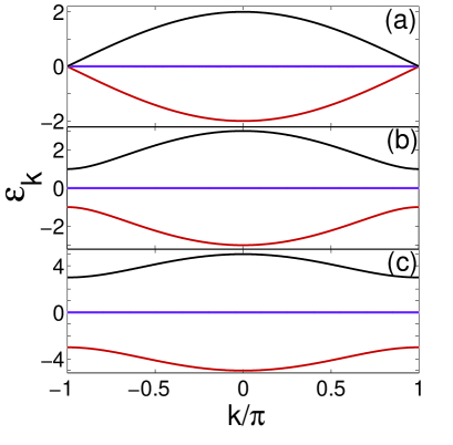
The case of angle $\theta=\pi/2$ in the 1D GCM is special and will be considered in more detail below. The structure of the Hilbert space gives here a macroscopic degeneracy of $2^{N/2-1}$ away from the isotropic point, and the enhanced degeneracy of $2^{N/2}$ when the orbital interactions are isotropic, i.e., $J_{\rm e}=J_{\rm o}$. We recall that we use here odd numbers of $k$ values included in the chosen set given by Eq. (12), and only in the thermodynamic limit we recover the degeneracy of $2\times 2^{N/2}$ for isotropic interactions Brz07 . Using fermions after the Jordan-Wigner transformation, this degeneracy is due to the acoustic branch which has no dispersion and is found at zero energy, $\varepsilon_{k,1}=0$, see Fig. 2. Then this branch is half-filled by fermions as it becomes degenerate with the one of negative energy $-\varepsilon_{k,1}$. Therefore, using the fermionic language one recovers here a macroscopic $2^{N/2}$ degeneracy of the ground state in the thermodynamic limit, independently of the mutual values of exchange parameters, and one finds for $J_{\rm e}\neq J_{\rm o}$ that $\forall k$: $\varepsilon_{k,1}<\varepsilon_{k,2}$, see Figs. 2(b) and 2(c). The gap at $k=\pi$ is given by the anisotropy of the pseudospin exchange, $\Delta=|J_{\rm e}-J_{\rm o}|$. The situation changes, however, when $J_{\rm e}=J_{\rm o}$ and the gap between $\varepsilon_{\pi,2}$ and $\varepsilon_{\pi,1}$ closes, see Fig. 2(a). This implies that the degeneracy increases by an additional factor of 2 due to the band-edge points.

Figure 3: (Color online) The gap $\Delta$ as a function of $\theta$ and $h$. The dotted line is the critical line given by Eq. (44). Parameters: $J_{\rm o}=1$, $J_{\rm e}=4$.

Figure 4: (Color online) The electronic QP energies $\pm\varepsilon_{k,n}/2$ ($n=1,2$) as obtained for the QCM Eq. (39) at finite polarization field (6): (a) $h=1$, and (b) $h=2$. In both cases the lower two bands are filled by fermions and a finite gap separates occupied from empty bands. Parameters: $J_{\rm o}=1$, $J_{\rm e}=4$, and $\theta=\pi/2$.

High degeneracy of the ground state is removed by finite field $h>0$. For $\theta\neq\pi/2$, Eq. (37) reduces to,

$$h_{c}=\pm 2\cos\theta\sqrt{J_{\rm o}J_{\rm e}}.$$ (44)

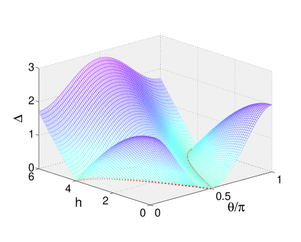
It defines the critical field at which the gap closes, see Fig. 3.

As $h$ approaches $h_{c}$, the gap vanishes as $\Delta\sim(h-h_{c})^{\nu z}$, where $\nu$ and $z$ are the correlation-length and dynamic exponent, respectively. The gap near criticality is

$$\Delta\simeq\frac{h^{2}-h_{c}^{2}}{2(J_{\rm o}+J_{\rm e})},$$ (45)

and one finds the critical exponent $\nu z=1$. In this sense, the 1D QCM has Ising-type long range order for finite $\theta<\pi/2$ and $h<h_{c}$. This is in analogy to the Ising model in transverse magnetic field, where a similar transition was reported Dzi05 . We emphasize that the phase space of the orbital liquid consists thus of a plane in the parameter space, spanned by $\{J_{\rm e},J_{\rm o}\}$.

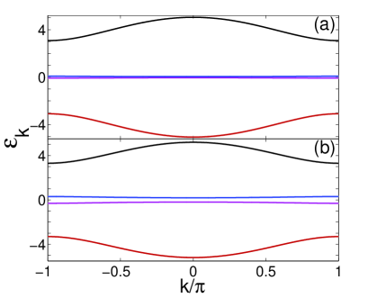
The critical lines intersect at $\theta_{c}=\pi/2$ and $h_{c}=0$, forming a multicritical point, where the model is gapless irrespective of the values of $J_{\rm e}$ and $J_{\rm o}$, see Fig. 3. It has been proven that the 90^∘ quantum compass model is critical for arbitrary ratio $J_{\rm e}/J_{\rm o}$ and the point $J_{\rm e}=J_{\rm o}$ corresponds to a multicritical point Eri09 . Finite field $h$ polarizes orbitals and removes high degeneracy of the ground state. For the fermionic QP bands this means that a gap at the Fermi energy opens exponentially between the bands $\varepsilon_{k,1}$ and $-\varepsilon_{k,1}$, and the system turns into an insulator, see Fig. 4. The gap is much smaller than the field $h$ and therefore the thermal excitations through the gap contribute to the thermodynamic properties at relatively low temperature as we show below in Sec. IV.

III.2 Orbital order and correlation functions at finite field

Frustrated interactions in Eq. (38) result in disordered state and the longitudinal polarization vanishes at $T=0$, i.e., $\langle\sigma_{i}^{x}\rangle=\langle\sigma_{i}^{y}\rangle=0$. The transverse polarization,

$${\cal P}=N\langle\sigma_{i}^{z}\rangle,$$ (46)

is induced by finite field $h$ at $T=0$; it is found with help of Hellmann-Feynman theorem,

$${\cal P}=-\frac{\partial E_{0}}{\partial h}.$$ (47)

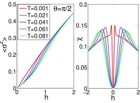
A similar thermodynamic relation which involves the total spectrum via the free energy ${\cal F}$ is used to determine $\langle\sigma_{i}^{z}\rangle$ at finite $T>0$ in Sec. IV. The order parameter $\langle\sigma_{i}^{z}\rangle$ is induced by the transverse field $h$, as shown in Fig. 5. By investigating the behavior of $\langle\sigma_{i}^{z}\rangle$ with increasing field $h$, we establish that the field-induced QPT is here second order for any angle $\theta$ Sun09 . It is also accompanied by a scaling behavior since the correlation length diverges and there is no characteristic length scale in the system at the critical point.

Figure 5: (Color online) Orbital polarization $\langle\sigma^{z}\rangle$ obtained for the GCM with increasing field $h$ in the ground state for different values of $\theta$. Parameters: $J_{\rm o}=1$, $J_{\rm e}=4$.

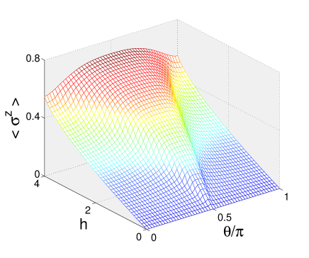
However, one finds a qualitatively different behavior at finite field $h$ for the GCM with interactions at $\theta<\pi/2$ (which includes the EOM) from that at $\theta=\pi/2$ for the QCM. The disordered phase in the QCM may easily be polarized by the field, while the ground state is more robust away from this point. In this regime the model has Néel order induced by the $x$-th pseudospin components (Ising order for the strongest interaction) and is harder to be destroyed by the transverse field. The results shown in Fig. 5 are confirmed by exact diagonalization that we performed on finite clusters in addition. Increasing transverse field induces finite $\langle\sigma_{i}^{z}\rangle$ and drives the system into a saturated polarized phase found above the critical field, i.e., for $h>h_{c}$.

Figure 6: (Color online) The 3D panorama of the NN orbital correlations, shown as functions of angle $\theta$ and the transverse field $h$ on odd bonds: (a) $-\langle\sigma_{2i-1}^{x}\sigma_{2i}^{x}\rangle$, and (b) $-\langle\sigma_{2i-1}^{y}\sigma_{2i}^{y}\rangle$. Parameters: $J_{\rm o}=1$ and $J_{\rm e}=4$.

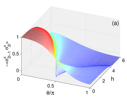
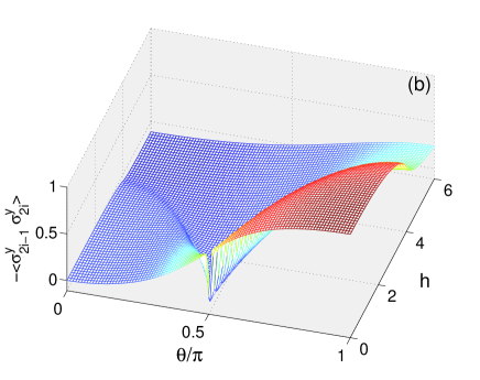
Two-point correlation functions which correspond to the dominating interaction decay algebraically with distance $r$ Brz07 . They are given by Osb02 :

$$\langle\sigma_{0}^{x}\sigma_{r}^{x}\rangle = \left|\begin{array}[]{c c c c}G_{-1}&G_{-2}&\cdot&G_{-r}\\ G_{0}&G_{-1}&\cdot&G_{-r+1}\\ \vdots&\vdots&\ddots&\vdots\\ G_{r-2}&G_{r-3}&\cdot&G_{-1}\end{array}\right|,$$ (52)

$$\langle\sigma_{0}^{y}\sigma_{r}^{y}\rangle = \left|\begin{array}[]{c c c c}G_{1}&G_{0}&\cdot&G_{-r+2}\\ G_{2}&G_{1}&\cdot&G_{-r+3}\\ \vdots&\vdots&\ddots&\vdots\\ G_{r}&G_{r-1}&\cdot&G_{1}\end{array}\right|,$$ (57)

$$\langle\sigma_{0}^{z}\sigma_{r}^{z}\rangle = 4\langle\sigma^{z}\rangle^{2}-G_{r}G_{-r},$$ (58)

where we have introduced the short-hand notation for the mixed correlation function,

$$G_{r}=\langle\sigma_{0}^{y}\sigma_{r}^{x}\rangle.$$ (59)

The numerical analysis shows two distinct phases at $h=0$, with large either $-\langle\sigma_{2i-1}^{x}\sigma_{2i}^{x}\rangle$ or $-\langle\sigma_{2i-1}^{y}\sigma_{2i}^{y}\rangle$, depending on whether $\theta<\pi/2$ or $\theta>\pi/2$. Note that NN orbital correlations are almost classical in a broad range of $\theta$ at $h=0$ as the model is Ising-like. The correlations decrease, however, when the quantum critical point (QCP) at $\theta=\pi/2$ is approached Brz07 . At this point one finds the disordered orbital state and the role of XX and YY correlations is interchanged, see Fig. 6. In both phases at $\theta\neq\pi/2$ there is a gap in the excitation spectrum which vanishes at the critical field ($h$=$h_{c}$), together with a jump in transverse magnetization shown in Fig. 5 and in the NN orbital correlation functions in Fig. 6 at $h_{c}(\theta)$.

We remark that the vanishing of the intersite correlators between uncoupled orbitals in the 1D QCM follows indeed from the local $Z_{2}$ symmetry, see the Appendix, and may also be seen as a consequence of Elitzur’s theorem — similar as in case of the 2D Kitaev model on a hexagonal lattice Che08 . One may also employ the general approach of ”bond algebra” Nus09 which leads to the same conclusion.

IV Finite temperature properties

IV.1 The entropy and the cooling rate

Having the exact solution of the GCM (38), it is straightforward to obtain its full thermodynamic properties at finite temperatures. For the particle-hole excitation spectrum (34), we determined the free energy of the quantum spin chain per site (here and below we take the Boltzmann constant $k_{\rm B}\equiv 1$),

$${\cal F}=-T\sum_{k}\sum_{j=1}^{2}\ln\left(2\cosh\frac{\varepsilon_{k,j}}{2T}\right).$$ (60)

Entropy ${\cal S}$ provides information about the evolution of spectra with increasing transverse field $h$. It has been determined from the free energy ${\cal F}$ (60) via the usual thermodynamic relation,

$${\cal S} \!= -\left(\frac{\partial{\cal F}}{\partial T}\right)_{V}$$

$$\!= \!\sum_{k}\sum_{j=1}^{2}\ln\left(2\cosh\frac{\varepsilon_{k,j}}{2T}\right)-\sum_{k}\sum_{j=1}^{2}\left(\frac{\varepsilon_{k,j}}{2T}\tanh\frac{\varepsilon_{k,j}}{2T}\right).$$

Figure 7: (Color online) The entropy ${\cal S}$ per unit cell for increasing field $h$ at different temperature $T=0.01,0.02,\cdots 0.10$ (from bottom to top) for two values of $\theta$: (a) the EOM ($\theta=\pi/3$), and (b) the QCM ($\theta=\pi/2$), corresponding to the critical field $h_{c}$=2 and 0, respectively. Insets show the temperature scaling of entropy for the critical field (top lines) and for the noncritical case (bottom lines). Parameters: $J_{\rm o}=1$, $J_{\rm e}=4$.

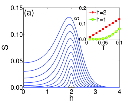
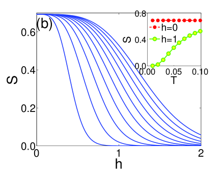
For the EOM, the entropy vanishes at $h=0$ and at $T=0$. It grows with increasing $T$ when thermal excitations gradually include more and more of excited states and this increase is faster at finite field, for instance finite entropy is found already at $T>0.05$ if $h=1$, see inset in Fig. 7(a). The entropy displays a distinct maximum for increasing transverse field at $h\simeq h_{c}$, where the gap closes, see Fig. 7(a), implying the QCP. This accumulation of entropy close to the QCP indicates that the states which characterize competing phases are almost degenerate and the system is ”maximally undecided” which ground state to choose Wu11 . The landscape of ${\cal S}$ defines the quantum critical regime, where $T\gg\Delta$ and role played by quantum and thermal fluctuations is equally important for the dynamics Sac00 . Especially, the system is gapless along the critical line and the entropy is linear in $T$, i.e., ${\cal S}\propto T$ for low temperatures, while in the gapped phases an exponential behavior, i.e., ${\cal S}\propto\exp(-\Delta/T)$ is observed.

Figure 8: (Color online) Lines of constant entropy ${\cal S}$ per unit cell, i.e., adiabatic demagnetization curves of the extended QCM in a transverse transverse field, as obtained for: (a) the EOM ($\theta=\pi/3$), and (b) the QCM ($\theta=\pi/2$). The QCP at $T=0$ gives a very distinct behavior in both cases near the critical field, being $h_{c}=2$ for the EOM (a), and $h_{c}=0$ for the QCM (b). In case (b) the field $h$ corresponding to a constant entropy exhibits a logarithmic increase with temperature below $T^{*}$. Parameters: $J_{\rm o}=1$, $J_{\rm e}=4$.

In the 1D QCM one finds a different behavior, see Fig. 7(b). The entropy ${\cal S}$ approaches here $\ln 2$ which follows from the high degeneracy $2^{N/2-1}$ of the disordered ground state. At $h=0$ one finds here a macroscopic entropy ${\cal S}\simeq\ln 2$ per unit cell that does not change with increasing temperature $T$ over a temperature range below the crossover temperature $T^{*}$, see below.

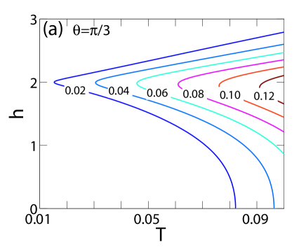
The qualitative difference between the EOM and the 1D QCM is best illustrated by the lines of constant entropy. The entropy ${\cal S}$ vanishes for the EOM at $T=0$, see Fig. 8(a), where the strongest interactions impose the quasi-order in the ground state. This follows the third law of thermodynamics which states that for pure and uniform phases the entropy falls to zero at $T\to 0$. However, in the vicinity of $h_{c}=2$ it increases fast with increasing $T$.

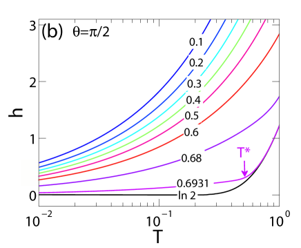
In contrast, the entropy for the QCM is maximal, ${\cal S}_{\rm max}=\ln 2$, at the QCP at $h_{c}=0$, and finite $h$ reduces ${\cal S}$ rapidly. In the vicinity of the QCP the field corresponding to a constant entropy exhibits a logarithmic increase with temperature, $h\propto\ln T$, see Fig. 8(b). This behavior demonstrates that the high degeneracy of the ground state is reduced by the external field which selects only certain states with their symmetry adapted to the field. A similar reduction of the ground state degeneracy is found in the 2D QCM when the added Heisenberg spin couplings induce magnetic long-range order Tro10 .

The entropy in the QCM is almost insensitive to increasing temperature, but the field quenches the spin disorder leading to a crossover to the classical state. These features could be the subject of future experimental studies. Recently, the complete entropic landscape was quantitatively measured for Sr₃Ru₂O₇ under transverse field in the vicinity of quantum criticality Rost09 . More interestingly, the low-entropy state has been a grand concern in realizing some exotic phases in optical lattice such as $d$-wave superconductivity Ho09 ; McK11 .

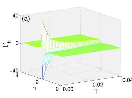
The field-induced QPT leads to universal responses when the applied field is varied adiabatically, and the magnetocaloric effect (MCE) can be used to study their quantum criticality. The adiabatic demagnetization curves of extended quantum models, ${\cal S}(h,T)={\rm const}$, are shown in Fig. 8. The MCE is closely related to the generalized cooling rate defined as follows,

$$\Gamma_{h}=-\frac{1}{T}\frac{(\partial{\cal S}/\partial h)_{T}}{(\partial{\cal S}/\partial T)_{h}}=\frac{1}{T}\left(\frac{\partial T}{\partial h}\right)_{\cal S}.$$ (62)

Figure 9: (Color online) The cooling rate $\Gamma_{h}$ Eq. (62) as obtained for increasing field $h$ and temperature $T$ at: (a) $\theta=\pi/3$, and (b) $\theta=\pi/2$. Parameters: $J_{\rm o}=1$, $J_{\rm e}=4$.

Generally, the variation of entropy ${\cal S}$ with external field $h$ is more singular than that of the specific heat considered in Sec. IV.2, so one expects that the MCE Eq. (62) is particularly large in the vicinity of the QCP. Near a field-tuned QCP, the critical part of the free energy takes usually the hyperscaling form in $d$ dimensions Zhu03 , $F=F_{0}T^{d/z+1}f(x/T^{1/\nu z})$, where $x=h-h_{c}$. The universal function $f(x)$ has diverse asymptotic behaviors in the $x\to 0$ and $x\to\pm\infty$ limits, respectively, corresponding to the quantum critical and quantum disordered/renormalized classical regimes. This divergent behavior at the QCP obeys a universal scaling law Zhu03 ,

$$\Gamma_{h}(T\to 0,h)=-\,G_{h}\,\frac{1}{h-h_{c}},$$ (63)

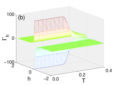
where a universal amplitude $G_{h}=1$ is found. This value is expected for a $Z_{2}$ symmetry in one dimension. In the opposite limit, $\Gamma_{h}\sim 1/T^{1/\nu z}$ for $x\ll T$. The $1/x$ divergence in the low temperature limit amounts to a sign change of $\Gamma_{h}$ as entropy accumulates near a QCP, as shown in Fig. 9(a). Therefore, the critical fields are pinpointed by sign changes of $\Gamma_{h}$ from negative to positive values upon increasing field. As the temperature is raised, the discontinuity at $h_{c}$ is rapidly reduced and all the distinct features seen at $T=0$ gradually disappear.

The dependence of the cooling rate on $h$, found for the disordered ground state of the QCM (at $\theta=\pi/2$), is qualitatively different, see Fig. 9(b). One finds here sharp and pronounced positive and negative peaks which occur at the transition point $h_{c}=0$, and this structure is robust, i.e., the strength of these peaks does not vary upon increasing temperature until a critical value is reached. The strong enhancement of the MCE arising from quantum fluctuations near a $h$-induced QCP can be used for finding an efficient and flexible high performance field cooling over an extended temperature range.

Figure 10: (Color online) The 3D plot of the specific heat $C_{V}$ normalized per unit cell for the: (a) EOM at $\theta=\pi/3$, and (b) QCM at $\theta=\pi/2$. Note that the specific heat reaches its local minima at QCPs only for extremely low temperatures. Parameters: $J_{\rm o}$=1, $J_{\rm e}$=4.

IV.2 Specific heat for the 1D compass models

Next we analyze the low temperature behavior of the heat capacity,

$$C_{V} = T\left(\frac{\partial{\cal S}}{\partial T}\right)_{h}=\sum_{k}\sum_{j=1}^{2}\frac{\varepsilon_{k,j}^{2}}{4T^{2}\cosh^{2}(\varepsilon_{k,j}/2T)}.$$ (64)

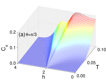
We recall that the entropy exhibits fast changes when the field $h$ is close to its critical value, $h\approx h_{c}$ (but $h\neq h_{c}$), see Fig. 7. Here we concentrate on the qualitative differences between the EOM and the QCM. The specific heat for both models is presented in 3D plots, for increasing temperature and transverse field, see Fig. 10. We have found that the low temperature behavior exhibits striking differences between these models discussed below.

Consider first the EOM of Sec. II.1 [with angle $\theta=\pi/3$ in Eq. (38)]. The specific heat contains here a broad peak around $h_{c}=2$ which corresponds to the QCP, and grows with increasing temperature. This demonstrates that more entropy is released here, as the spectrum of excited states is dense near $h\simeq h_{c}$. Furthermore, $C_{V}$ develops a local minimum which splits the peak at $h\simeq h_{c}$ into two separate maxima for extremely low temperatures, see Fig. 10(a). The maxima seen at $h<h_{c}$ and $h>h_{c}$ are of different height which reflects the different spectra and increase of entropy with increasing temperature in the vicinity of the QCP at $h_{c}=2$. The shallow trough in heat capacity can be linked with orbital susceptibility discussed in Sec. IV.3 by the Maxwell relation Jaf12 .

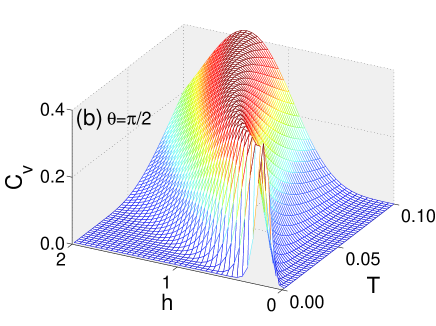
In contrast, increasing temperature at the QCP of the QCM ($h=h_{c}=0$) does not result in any increase of the specific heat and one finds $C_{V}=0$ in a broad range of temperature, see Fig. 10(b). This somewhat surprising behavior is a consequence of the gap between the excited states and the ground state. Here the ground state has high macroscopic degeneracy, being $d=2^{N/2-1}$ — this degenerate state is a robust feature of the QCM, responsible for its rather unusual properties, see also Sec. IV.3. Finite transverse field $h$, however, splits the ground state multiplet, and the entropy at low temperature decreases, see Fig. 7(b). Increasing temperature for a constant but finite field $h$ results then in a fast increase of entropy which is responsible for a large maximum in $C_{V}$ for the QCM, as observed in Fig. 10(b).

IV.3 Orbital polarization and susceptibility

In this Section we analyze the orbital properties at finite polarizing field $h$ of both the EOM and QCM at finite temperature near the QPT. From the free energy ${\cal F}$ we determined the orbital polarization ${\cal P}$ along the transverse field,

$${\cal P}=-\left(\frac{\partial{\cal F}}{\partial h}\right)_{T}=\sum_{k}\sum_{j=1}^{2}\frac{\partial\varepsilon_{k,j}}{\partial h}\tanh\left(\frac{\varepsilon_{k,j}}{2T}\right),$$ (65)

which vanishes as $h\to 0$. Thus, there is no polarization at any finite temperature in one dimension and no nontrivial critical point, in accordance with the Mermin-Wagner theorem. Also, there are no peculiarities of the order parameter $\langle\sigma^{z}\rangle$ at any finite temperature and finite transverse field $h$.

Figure 11: (Color online) Orbital response in a transverse field $h$ for the EOM at different temperatures: (a) the orbital polarization $\langle\sigma^{z}\rangle$ per site, and (b) the orbital susceptibility $\chi$ per site (66). The QPT is found at $h_{c}=2$. Different curves from top to bottom correspond to increasing temperature and are normalized per one site. Parameters: $J_{\rm o}$=1, $J_{\rm e}$=4, $\theta=\pi/3$.

Figure 12: (Color online) Orbital response in a transverse field $h$ for the QCM at different temperature: (a) polarization $\langle\sigma^{z}\rangle$ per site, and (b) the orbital susceptibility $\chi$ per site (66). Different curves from the center to the left or right correspond to increasing temperature and are normalized per one site. Parameters: $J_{\rm o}$=1, $J_{\rm e}$=4, $\theta=\pi/2$.

The orbital susceptibility is the derivative of the polarization ${\cal P}$ (46) over the field $h$, and we define it here per one site,

$$\chi=\frac{1}{N}\left(\frac{\partial{\cal P}}{\partial h}\right)_{T}=\left(\frac{\partial\langle\sigma_{i}^{z}\rangle}{\partial h}\right)_{T}.$$ (66)

After using the Jordan-Wigner fermions one finds it in the fermionic representation,

$$\chi = \frac{1}{2N}\sum_{k}\sum_{j=1}^{2}\left\{\frac{\partial^{2}\varepsilon_{k,j}}{\partial h^{2}}\tanh\left(\frac{\varepsilon_{k,j}}{2T}\right)\right.$$ (67)

$$+ \left.\left(\frac{\partial\varepsilon_{k,j}}{\partial h}\right)^{2}\left[2T\cosh^{2}\left(\frac{\varepsilon_{k,j}}{2T}\right)\right]^{-1}\right\}.$$

We emphasize that the orbital properties (similar to magnetic properties in spin models) are intimately related to the field dependence of the entropy via the Maxwell identity,

$$\left(\frac{\partial{\cal S}}{\partial h}\right)_{T}=\left(\frac{\partial{\cal P}}{\partial T}\right)_{h},$$ (68)

which allows to rewrite the cooling rate as

$$\Gamma_{h}=\frac{1}{C_{V}}\left(\frac{\partial{\cal P}}{\partial T}\right)_{h}.$$ (69)

Therefore, we discuss below the orbital properties from the perspective of the peculiarities of the entropy at finite field and finite temperature, presented in Sec. IV.1.

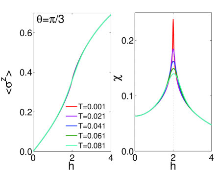
The polarization $\langle\sigma^{z}\rangle$ of the EOM increases with field $h$ and this increase is almost independent of temperature except in the vicinity of the phase transition, see Fig. 11(a). At the critical field $h_{c}=2$ the derivative of the polarization diverges at $T=0$, and in the low temperature regime one finds a sharp maximum in the susceptibility $\chi$ at $h=h_{c}$, see Fig. 11(b). This behavior represents a generic QPT with $h$ as control parameter. We note that the associated peak in the entropy leading to the phase transition is described here by the vanishing of the gap $\Delta$ Eq. (36) that occurs in the fermionic spectrum at $h=h_{c}$.

Figure 13: (Color online) The 3D plot of the orbital susceptibility $\chi$ (66) versus temperature and field for the: (a) EOM at $\theta=\pi/3$, and (b) QCM at $\theta=\pi/2$. Parameters: $J_{\rm o}$=1, $J_{\rm e}$=4. The EOM (a) shows a QPT at finite field $h_{c}=2$. The QCM (b) is characterized by the macroscopic degeneracy of the low energy sector and vanishing $\chi$ at zero field, while finite $h$ lifts the degeneracy and leads to a peak in $\chi$.

The 1D QCM shows a remarkably different orbital response. Here the polarization increase with $h$ depends strongly on temperature, see Fig. 12(a). A clearer presentation of this peculiar behavior is possible in terms of the susceptibility $\chi$, Fig. 12(b). Here $\chi(T,h)$ vanishes at $h=0$ and acquires a peak at a finite field $h_{m}(T)$ which increases with temperature. This is another manifestation of the macroscopic entropy at zero temperature, shown in Fig. 7(b), that stems from the highly degenerate ground state. In the fermionic language the vanishing of $\chi$ at $h=0$ is connected with the high degeneracy of the subspace described by two dispersionless half-filled fermionic bands, $\pm\epsilon_{k,1}=0$. When the degeneracy is lifted by a finite transverse field, the entropy changes dramatically and causes a rapid increase of the susceptibility shown in Fig. 12(b). Below we shall discuss a different picture for the origin of this degeneracy in the QCM.

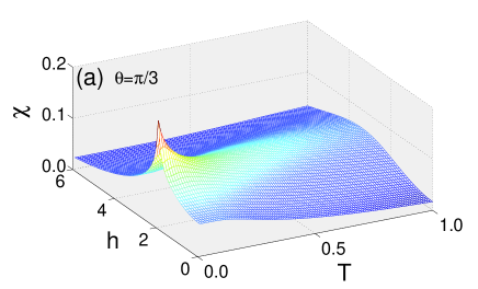
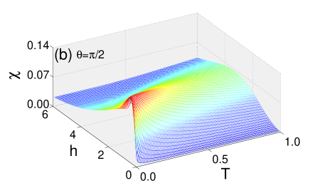
Finally, we compare the orbital susceptibility $\chi$ (67) obtained for both 1D compass models (the EOM and the QCM) in a broad range of temperature in Fig. 13. In the gapped phase of the EOM at $h=0$, the low temperature orbital susceptibility is finite and decreases with increasing $T$ for the unpolarized system, see Fig. 13(a). In contrast, one finds a vanishing orbital susceptibility at the critical point of the QCM $h=0$ in a broad range of temperature. A distinct maximum develops close to $h=0$ at low temperature — this maximum moves to higher field and looses intensity when temperature increases further, see Fig. 13(b). All these distinct features emphasize once again radical difference between the nature of the QPTs found in both compass models.

V Discussion and summary

In this paper we explored the ground state and the thermodynamic properties of the 1D generalized compass model with exchange interactions given by Eq. (3), and tuned by an angle $\theta$. They vary from Ising interactions at $\theta=0$ to maximally frustrated ones with two different pseudospin components coupled on even/odd bonds at $\theta=\pi/2$ in the quantum compass model. In between (at $\theta=60^{\circ}$) one finds the $e_{g}$ orbital model. In this way, we investigated the consequences of increasing frustration of spin interactions in one dimension. The model was solved exactly and we presented its exact characteristics in the thermodynamic limit: the entropy, the specific heat, the orbital susceptibility, and the adiabatic demagnetization curves. By investigating the dependence of all these quantities on the angle $\theta$, we have shown that the ground state is ordered along the easy axis as long as $\theta\neq\pi/2$, whereas it becomes disordered and highly degenerate at $\theta=\pi/2$, i.e., when the interacting pseudospin components along even/odd bonds are orthogonal.

Pseudospin excitations are separated by a gap from the ground state everywhere except for the quantum compass model, where the gap closes and one finds a highly disordered spin-liquid ground state. This demonstrates an important difference between the $e_{g}$ orbital model with favored type of short-range order and the quantum compass model in one dimension. While the above order for the $e_{g}$ orbitals is analogous to the 2D case Cin10 , the 1D compass model fails to develop the nematic order known from its 2D analog.

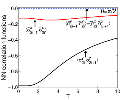
The generic temperature dependence of pseudospin correlations on the bonds in the 1D quantum compass model is summarized in Fig. 14. Only these pseudospin correlations take finite values which are coupled by finite interaction parameters, similar as in the isotropic case Brz07 . As expected, at $T=0$ the value of pseudospin correlation $|\langle\sigma_{2i}^{y}\sigma_{2i+1}^{y}\rangle|$ is larger than $|\langle\sigma_{2i-1}^{x}\sigma_{2i}^{x}\rangle|$ as the first one corresponds to a stronger interaction. On the other hand, the complementary orbital correlations for pairs that are not coupled by any interaction, i.e., $\langle\sigma_{2i}^{x}\sigma_{2i+1}^{x}\rangle$ and $\langle\sigma_{2i-1}^{y}\sigma_{2i}^{y}\rangle$, vanish and this follows from the $Z_{2}$ symmetry Che08 , as discussed also in the Appendix. Note that a finite value of $\langle\sigma_{2i-1}^{x}\sigma_{2i}^{x}\rangle$ in Fig. 14 is a manifestation of the quantum nature of the compass model, as in the classical case one finds instead only finite pseudospin correlations on stronger bonds, i.e., $\langle\sigma_{2i}^{y}\sigma_{2i+1}^{y}\rangle=-1$ and $\langle\sigma_{2i-1}^{x}\sigma_{2i}^{x}\rangle=0$.

Figure 14: (Color online) Nearest neighbor pseudospin correlations in the anisotropic quantum compass model [the model Eq. (38) with angle $\theta=\pi/2$ and stronger coupling of $\{\sigma_{i}^{y}\}$ components on the even bonds] for increasing temperature $T$. Only the intersite correlation corresponding to the interacting pseudospin components are finite. Parameters: $J_{\rm o}=1$, $J_{\rm e}=4$.

Furthermore, we have shown that the external transverse field has also quite different consequences, depending on the underlying interactions. In the $e_{g}$ orbital model intersite pseudospin correlations are robust and follow the strongest interactions. Therefore, a significant value of the transverse field is required here to modify the short-range correlations, dictated by the $\sigma_{i}^{x}\sigma_{i+1}^{x}$ interactions, and to induce the polarized state. A qualitatively different situation is encountered in the quantum compass model. Here the highly disordered ground state is fragile and already an infinitesimal transverse field destabilizes it and induces a quantum phase transition which we recognized as being of second order by investigating the adiabatic demagnetization at finite temperature. The observed behavior corresponds to entropy maximization at the quantum critical point in the low-temperature limit. The high degeneracy revealed by finite entropy at low temperature suggests that the 90^∘ compass model may have potential application in quantum computation Rio11 . In addition, the cooling rate in the quantum compass model could be testified in the state-of-the-art experiments at optical lattice McK11 .

We would like to emphasize that some quantum integrable 1D models were developed in the past to provide valuable insights into the nature of quantum correlations in the ground state, as well as into the structure of excited states. Such models: (i) help to understand the nature of many-body states in such models, and (ii) provide a possibility to test approximate theoretical methods used for more realistic physical models of frustrated spin interactions, in two and three dimensions. The present study should serve the same purpose.

Summarizing, we have demonstrated that robust pseudospin correlations arise on the bonds in the $e_{g}$ orbital model — these correlations get destroyed only at the quantum phase transition which occurs at rather strong transverse field. On the contrary, the disordered spin-liquid state in the isotropic quantum compass model is fragile and gets destroyed by infinitesimal field. A qualitative difference is found for anisotropic interactions — the spin-liquid state is more robust here and survives up to temperature $T^{*}$ which appears to be a new energy scale and increases with increasing anisotropy of interactions. This feature follows from the weak logarithmic decrease of spin entropy with increasing temperature, and persisting high degeneracy of the ground state in this temperature range.

Appendix A Consequences of the $Z_{2}$ symmetry

In this Appendix we shall show that the macroscopic degeneracy of the 1D QCM which was manifested in two fermionic bands at zero energy, $\pm\varepsilon_{k}=0$, is due to local $Z_{2}$ symmetries of the model in the absence of the transverse field term. For this discussion we write the QCM Eq. (39) in an equivalent form with simplified notation,

$${\cal H}_{\rm QCM}=-\sum_{i}(J_{x}\sigma^{x}_{2i-1}\sigma^{x}_{2i}+J_{z}\sigma^{z}_{2i}\sigma^{z}_{2i+1}),$$ (70)

and introduce operators which act on bonds note1D :

$$X_{i} = \sigma^{x}_{2i}\sigma^{x}_{2i+1},$$ (71)

$$Z_{i} = \sigma^{z}_{2i-1}\sigma^{z}_{2i},$$ (72)

where each set of operators, $i=1,2,.....,N/2$, commutes with the Hamiltonian. Thus we can use the tuple

$$\vec{Z}\equiv(Z_{1},...,Z_{i},....,Z_{N/2})$$ (73)

to classify the eigenstates of ${\cal H}_{\rm QCM}$, for instance

$${\cal H}_{\rm QCM}|\Phi_{0}\rangle = \varepsilon_{0}|\Phi_{0}\rangle,$$ (74)

$$\vec{Z}|\Phi_{0}\rangle = (\lambda_{1},...,\lambda_{i},....,\lambda_{N})|\Phi_{0}\rangle,$$ (75)

where the eigenvalues $\lambda_{i}=\pm 1$ follow from $Z_{i}^{2}=1$. It is important to recognize that the operators $Z_{i}$ and $X_{j}$ anticommute for special cases:

$$\{Z_{i},X_{i}\} = 0,$$ (76)

$$\{Z_{i},X_{i-1}\} = \{Z_{i+1},X_{i}\}=0,$$ (77)

while they commute otherwise. We note here, that the key difference to the 2D QCM Dou05 ; Dor05 ; Tro10 lies in the different form of these anticommutation relations. Using the commutation relation $[{\cal H}_{\rm QCM},X_{i}]=0$, one finds that

$${\cal H}_{\rm QCM}X_{i}|\Phi_{0}\rangle=\varepsilon_{0}X_{i}|\Phi_{0}\rangle,$$ (78)

that is, also $|\Phi_{1}\rangle=X_{i}|\Phi_{0}\rangle$ is an eigenvector to the same eigenvalue $\epsilon_{0}$, and by analyzing the corresponding eigenvalue tupel $(\lambda_{1},...,\lambda_{i},....,\lambda_{N/2})$ one can convince oneself that this state is in fact distinct from $|\Phi_{0}\rangle$. One can now proceed by applying the same arguments to $|\Phi_{2}\rangle=X_{i-1}|\Phi_{0}\rangle$ and so on, until one exhausts all the $2^{N/2}$ states of the degenerate multiplet.

References

- (1) K. I. Kugel and D. I. Khomskii, JETP 37, 725 (1973); Sov. Phys. Usp. 25, 231 (1982).
- (2) L. F. Feiner, A. M. Oleś, and J. Zaanen, Phys. Rev. Lett. 78, 2799 (1997); J. Phys.: Condens. Matter 10, L555 (1998).
- (3) Y. Tokura and N. Nagaosa, Science 288, 462 (2000).
- (4) J. van den Brink, Z. Nussinov, and A. M. Oleś, in: Introduction to Frustrated Magnetism: Materials, Experiments, Theory, edited by C. Lacroix, P. Mendels, and F. Mila (Springer, New York, 2011).
- (5) A. M. Oleś, G. Khaliullin, P. Horsch, and L. F. Feiner, Phys. Rev. B 72, 214431 (2005).
- (6) G. Khaliullin, Prog. Theor. Phys. Suppl. 160, 155 (2005).
- (7) A. M. Oleś, J. Phys.: Condens. Matter 24, 313201 (2012).
- (8) G. Khaliullin, P. Horsch, and A. M. Oleś, Phys. Rev. Lett. 86, 3879 (2001); C. Ulrich, G. Khaliullin, J. Sirker, M. Reehuis, M. Ohl, S. Miyasaka, Y. Tokura, and B. Keimer, ibid. 91, 257202 (2003); P. Horsch, G. Khaliullin, and A. M. Oleś, ibid. 91, 257203 (2003); A. M. Oleś, P. Horsch, L. F. Feiner, and G. Khaliullin, ibid. 96, 147205 (2006); M. De Raychaudhury, E. Pavarini, and O. K. Andersen, ibid. 99, 126402 (2007); G. Khaliullin, P. Horsch, and A. M. Oleś, Phys. Rev. B 70, 195103 (2004); A. M. Oleś, P. Horsch, and G. Khaliullin, ibid. 75, 184434 (2007); P. Horsch and A. M. Oleś, ibid. 84, 064429 (2011); A. Avella, P. Horsch, and A. M. Oleś, ibid. 87, 045132 (2013); E. Benckiser, L. Fels, G. Ghiringhelli, M. Moretti Sala, T. Schmitt, J. Schlappa, V. N. Strocov, N. Mufti, G. R. Blake, A. A. Nugroho, T. T. M. Palstra, M. W. Haverkort, K. Wohlfeld, and M. Grüninger, ibid. 88, 205115 (2013).
- (9) J.-S. Zhou and J. B. Goodenough, Phys. Rev. Lett. 96, 247202 (2006); J.-S. Zhou, J. B. Goodenough, J.-Q. Yan, and Y. Ren, ibid. 99, 156401 (2007); P. Horsch, A. M. Oleś, L. F. Feiner, and G. Khaliullin, ibid. 100, 167205 (2008).
- (10) J. Sirker, A. Herzog, A. M. Oleś, and P. Horsch, Phys. Rev. Lett. 101, 157204 (2008); A. Herzog, P. Horsch, A. M. Oleś, and J. Sirker, Phys. Rev. B 83, 245130 (2011).
- (11) W.-L. You, A. M. Oleś, and P. Horsch, Phys. Rev. B 86, 094412 (2012); R. Lundgren, V. Chua, and G. A. Fiete, ibid. 86, 224422 (2012).
- (12) W. Brzezicki and A. M. Oleś, Phys. Rev. B 83, 214408 (2011); W. Brzezicki, J. Dziarmaga, and A. M. Oleś, Phys. Rev. Lett. 109, 237201 (2012); Phys. Rev. B 87, 064407 (2013).
- (13) W. Brzezicki, J. Dziarmaga, and A. M. Oleś, Phys. Rev. Lett. 112, LH14174 (2014).
- (14) G. Jackeli and G. Khaliullin, Phys. Rev. Lett. 102, 017205 (2009).
- (15) J. Chaloupka, G. Jackeli, and G. Khaliullin, Phys. Rev. Lett. 105, 027204 (2010); 110, 097204 (2013).
- (16) K. Wohlfeld, M. Daghofer, S. Nishimoto, G. Khaliullin, and J. van den Brink, Phys. Rev. Lett. 107, 147201 (2011); K. Wohlfeld, S. Nishimoto, M. W. Haverkort, and J. van den Brink, Phys. Rev. B 88, 195138 (2013).
- (17) J. Schlappa, K. Wohlfeld, K. J. Zhou, M. Mourigal, M. W. Haverkort, V. N. Strocov, L. Hozoi, C. Monney, S. Nishimoto, S. Singh, A. Revcolevschi, J.-S. Caux, L. Patthey, H. M. Rønnow, J. van den Brink, and T. Schmitt, Nature (London) 485, 82 (2012).
- (18) J. van den Brink, P. Horsch, F. Mack, and A. M. Oleś, Phys. Rev. B 59, 6795 (1999).
- (19) J. van den Brink, New J. Phys. 6, 201 (2004).
- (20) L. F. Feiner and A. M. Oleś, Phys. Rev. B 71, 144422 (2005).
- (21) A. van Rynbach, S. Todo, and S. Trebst, Phys. Rev. Lett. 105, 146402 (2010).
- (22) M. Daghofer, K. Wohlfeld, A. M. Oleś, E. Arrigoni, P. Horsch, Phys. Rev. Lett. 100, 066403 (2008); K. Wohlfeld, M. Daghofer, A. M. Oleś, P. Horsch, Phys. Rev. B 78, 214423 (2008); K. Wohlfeld, A. M. Oleś, M. Daghofer, P. Horsch, Acta Phys. Polon. A 115, 110 (2009).
- (23) P. Wróbel and A. M. Oleś, Phys. Rev. Lett. 104, 206401 (2010); P. Wróbel, R. Eder, and A. M. Oleś, Phys. Rev. B 86, 064415 (2012).
- (24) F. Trousselet, A. Ralko, and A. M. Oleś, Phys. Rev. B 86, 014432 (2012).
- (25) G. Chen and L. Balents, Phys. Rev. Lett. 110, 206401 (2013).
- (26) L. F. Feiner and A. M. Oleś, Phys. Rev. B 59, 3295 (1999).
- (27) F. Vernay, K. Penc, P. Fazekas, and F. Mila, Phys. Rev. B 70, 014428 (2004); A. J. W. Reitsma, L. F. Feiner, and A. M. Oleś, New J. Phys. 7, 121 (2005).
- (28) Z. Nussinov and J. van den Brink, arXiv:1303.5922 (unpublished).
- (29) Z. Nussinov and E. Fradkin, Phys. Rev. B 71, 195120 (2005).
- (30) B. Douçot, M. V. Feigel’man, L. B. Ioffe, and A. S. Ioselevich, Phys. Rev. B 71, 024505 (2005).
- (31) J. Dorier, F. Becca, and F. Mila, Phys. Rev. B 72, 024448 (2005).
- (32) H.-D. Chen, C. Fang, J.-P. Hu, and H. Yao, Phys. Rev. B 75, 144401 (2007).
- (33) S. Wenzel and W. Janke, Phys. Rev. B 78, 064402 (2008).
- (34) R. Orús, A. C. Doherty, and G. Vidal, Phys. Rev. Lett. 102, 077203 (2009).
- (35) L. Cincio, J. Dziarmaga, and A. M. Oleś, Phys. Rev. B 82, 104416 (2010).
- (36) W. Brzezicki and A. M. Oleś, Phys. Rev. B 82, 060401 (2010); Phys. Rev. B 87, 214421 (2013).
- (37) F. Trousselet, A. M. Oleś, and P. Horsch, Europhys. Lett. 91, 40005 (2010); Phys. Rev. B 86, 134412 (2012).
- (38) W. Brzezicki, J. Dziarmaga, and A. M. Oleś, Phys. Rev. B 75, 134415 (2007); W. Brzezicki and A. M. Oleś, Acta Phys. Polon. A 115, 162 (2009).
- (39) W. Brzezicki and A. M. Oleś, Phys. Rev. B 80, 014405 (2009).
- (40) A. Kitaev, Annals of Physics 321, 2 (2006).
- (41) H.-D. Chen and Z. Nussinov, J. Phys. A: Math. Theor. 41, 075001 (2008).
- (42) U. Divakaran and A. Dutta, Phys. Rev. B 79, 224408 (2009).
- (43) We take here instead of spin component in the EOM considered usually vdB99 .
- (44) Z. Nussinov, M. Biskup, L. Chayes, and J. van den Brink, Europhys. Lett. 67, 990 (2004).
- (45) M. Biskup, L. Chayes, and Z. Nussinov, Commun. Math. Phys. 255, 253 (2005).
- (46) E. Zhao and W. V. Liu, Phys. Rev. Lett. 100, 160403 (2008).
- (47) C. Wu, Phys. Rev. Lett. 100, 200406 (2008).
- (48) L. Longa and A. M. Oleś, J. Phys. A: Math. Gen. 13, 1031 (1980).
- (49) A. Mishra, M. Ma, F. C. Zhang, S. Guertler, L. H. Tang, and S. L. Wan, Phys. Rev. Lett. 93, 207201 (2004).
- (50) W.-L. You, G.-S. Tian, and H.-Q. Lin, Phys. Rev. B 75, 195118 (2007).
- (51) W.-L. You and G.-S. Tian, Phys. Rev. B 78, 184406 (2008).
- (52) W.-L. You, G.-S. Tian, and H.-Q. Lin, J. Phys. A: Math. Gen. 43, 275001 (2010).
- (53) P.-S. He, W.-L. You, and G.-S. Tian, Chin. Phys. B 20, 017503 (2011).
- (54) J. Vidal, R. Thomale, K. P. Schmidt, and S. Dusuel, Phys. Rev. B 80, 081104(R) (2009).
- (55) C. Xu and J. E. Moore, Phys. Rev. Lett. 93, 047003 (2004).
- (56) W.-L. You and Y.-L. Dong, Phys. Rev. B 84, 174426 (2011).
- (57) Wen-Long You, Eur. Phys. J. B 85, 83 (2012).
- (58) Ke-Wei Sun and Qing-Hu Chen, Phys. Rev. B 80, 174417 (2009).
- (59) Di Xiao, W. Zhu, Y. Ran, N. Nagaosa, and S. Okamoto, Nature Communications 2, 596 (2011).
- (60) J. Simon, W. S. Bakr, R. Ma, M. Eric Tai, P. M. Preiss, and M. Greiner, Nature (London) 472, 307 (2011).
- (61) G. Sun, G. Jackeli, L. Santos, and T. Vekua, Phys. Rev. B 86, 155159 (2012).
- (62) M. J. Konstantinović, J. van den Brink, Z. V. Popović, V. V. Moshchalkov, M. Isobe, and Y. Ueda, Phys. Rev. B 69, R020409 (2004).
- (63) T. Hikihara and Y. Motome, Phys. Rev. B 70, 214404 (2004).
- (64) J. Zaanen and A. M. Oleś, Phys. Rev. B 48, 7197 (1993).
- (65) P. G. Radaelli, New J. Phys. 7, 53 (2005).
- (66) R. Coldea, D. A. Tennant, E. M. Wheeler, E. Wawrzynska, D. Prabhakaran, M. Telling, K. Habicht, P. Smeibidl, and K. Kiefer, Science 327, 177 (2010).
- (67) K. Wohlfeld, M. Daghofer, and A. M. Oleś, Europhys. Lett. (EPL) 96, 27001 (2011).
- (68) J. Dziarmaga, Phys. Rev. Lett. 95, 245701 (2005).
- (69) E. Eriksson and H. Johannesson, Phys. Rev. B 79, 224424 (2009).
- (70) T. J. Osborne and M. A. Nielsen, Phys. Rev. A 66, 032110 (2002).
- (71) Z. Nussinov and G. Ortiz, Phys. Rev. B 79, 214440 (2009).
- (72) J. Wu, L. Zhu, and Q. Si, J. Phys.: Conf. Series 273, 012019 (2011).
- (73) S. Sachdev, Quantum Phase Transitions (Cambridge University Press, Cambridge, United Kingdom, 2000).
- (74) A. W. Rost, R. S. Perry, J.-F. Mercure, A. P. Mackenzie, and S. A. Grigera, Science 325, 1360 (2009).
- (75) T.-L. Ho, and Qi Zhou, PNAS 106, 6916 (2009).
- (76) D. McKay and B. DeMarco, Rep. Prog. Phys. 74 054401 (2011).
- (77) L. Zhu, M. Garst, A. Rosch, and Q. Si, Phys. Rev. Lett. 91, 066404 (2003).
- (78) R. Jafari, Eur. Phys. J. B 85, 167 (2012).
- (79) L. del Rio, J. Åberg, R. Renner, O. Dahlsten, and V. Vedral, Nature (London) 474, 61 (2011).
- (80) Such bond operators were introduced as pseudospins to classify the invariant subspaces in the 1D isotropic compass model Brz07 .