Disperse two-phase flows, with applications to geophysical problems

Abstract

In this paper we study the motion of a fluid with several dispersed particles whose concentration is very small (smaller than $10^{-3}$), with possible applications to problems coming from geophysics, meteorology, and oceanography. We consider a very dilute suspension of heavy particles in a quasi-incompressible fluid (low Mach number). In our case the Stokes number is small and –as pointed out in the theory of multiphase turbulence– we can use an Eulerian model instead of a Lagrangian one. The assumption of low concentration allows us to disregard particle–particle interactions, but we take into account the effect of particles on the fluid (two-way coupling). In this way we can study the physical effect of particles’ inertia (and not only passive tracers), with a model similar to the Boussinesq equations.

The resulting model is used in both direct numerical simulations and large eddy simulations of a dam-break (lock-exchange) problem, which is a well-known academic test case.
Keywords: Dilute suspensions, Eulerian models, direct and large eddy simulations, slightly compressible flows, dam-break (lock-exchange) problem.
MSC 2010 classification: Primary: 76T15; Secondary: 86-08, 86A04, 35Q35.

1 Introduction

One of the characteristic features of geophysical flows (see for instance [8]) is stratification (the other one is rotation). In this manuscript, we study some problems related to suspensions of heavy particles in incompressible -or slightly compressible- fluids. Our aim is a better understanding of mixing phenomena between the two phases, the fluid and solid one. We especially study this problem because (turbulent) mixing with stratification plays a fundamental role in the dynamics of both oceanic and atmospheric flows. In this study, we perform the analysis of some models related to the transport of heavy dilute particles, with special emphasis on their mixing. Observe that mixing is very relevant near the surface and the bottom of the ocean, near topographic features, near polar and marginal seas, as well as near the equatorial zones [21]. Especially in coastal waters, precise analysis of transport and dispersion is needed to study biological species, coastal discharges, and also transport of contaminants. The other main motivation of our study is a better understanding of transport of particles (e.g. dust and pollution) in the air. This happens -for instance- in volcanic eruptions or more generally by natural and/or human generation of jets/plumes of particles in the atmosphere.

Following [1], in the physical regimes we will consider, it is appropriate to use the Eulerian approach, that is the solid-phase (the particles) will be modeled as a continuum. This choice is motivated by the presence of a huge number of particles and because we are analyzing the so called “fine particle” regime (that is the Stokes number is much smaller than one). In this regime, a Lagrangian approach could be computationally expensive, and the Eulerian approach may offer more computationally efficient alternatives. We will explain the precise assumptions that make this ansatz physically representative and we will also study numerically the resulting models, with and without large scales further approximation. In particular, we will model the particles as dust, investigating a model related to dusty gases, and which belongs to the hierarchy of reduced multiphase models, as reviewed by Balachandar [1]. These models represent a good approximation when the number of fine particles to be traced is very large and a direct numerical simulation (DNS) of the fluid with a Lagrangian tracer for each particle would be too expensive. As well explained in [1], the point-like Eulerian approach for multiphase fluid-particle dynamics becomes even more efficient in the case of large eddy simulations (LES), because the physical diameter of the particles has to be compared with the large eddy length-scale and not with the smaller Kolmogorov one. We will use the dusty gas model in a physical configuration that is very close to that modeled by the Boussinesq system, and this explains why we compare our numerical results with those reported in [27, 2]. Observe that the dusty gas model reduces to the Boussinesq system with a large Prandtl number if: a) the fluid velocity is divergence-free; and b) the relative ratio of solid and fluid bulk densities is very small (see Sec. 2 and Eq. (6)).

The approach we will use for multiphase fluids is well-described in Marble [23]. More precisely, when the Stokes time –which is the characteristic time of relaxation of the particle velocity with respect to the surrounding fluid– is small enough and the number of particles is very large, it could be reasonable to use the Eulerian approach (instead of the Lagrangian). In Eulerian models both the carrier and the dispersed phase are treated as interpenetrating fluid media, and consequently both the particulate solid-phase and fluid-phase properties are expressed by a continuous field representation. Originally we started studying these models in order to simulate ash plumes coming from volcanic eruptions, see [10, 6, 5, 31], but here we will show that the same approach could be also used to study some problems coming from other geophysical situations, at least for certain ranges of physical parameters.

Our model is evaluated in a two dimensional dam-break problem, also known as the lock-exchange problem. This problem, despite being concerned with a) a simple domain; b) nice initial and boundary conditions; and c) smooth gravity external forcing, contains shear-driven mixing, internal waves, interactions with boundaries, and convective motions. The dam-break problem setup has long served as a paradigm configuration for studying the space-time evolution of gravity currents (cf. [9, 12, 28, 29]). Consequently, we set up a canonical benchmark problem, for which an extensive literature is available: The vertical barrier separating fluid and fluid with particles is abruptly removed, and counter-propagating gravity currents initiate mixing. The time evolution can be quite complex, showing shear-driven mixing, internal waves interacting with the velocity, and gravitationally-unstable transients. This benchmark problem has been investigated experimentally and numerically for instance in [3, 16, 17, 18]. Both the impressive amount of data and the physical relevance of the problem make it an appropriate benchmark and a natural first step in the thorough assessment of any approximate model to study stratification. The results we obtain validate the proposed model as appropriate to simulate dilute suspensions of ash in the air. In addition, we found that new peculiar phenomena appear, which are generated by compressibility. Even if the behavior of the simulations is qualitatively very close to that of the incompressible case, the (even very slightly) compressible character of the fluid produces a more complex behavior, especially in the first part of the simulations. To better investigate the efficiency and limitations of the numerical solver, the numerical tests will be performed by using both DNS and LES. Complete discussion of the numerical results will be given in Section 3.

Plan of the paper: In Section 2 we present the reduced multiphase model we will consider, with particular attention to the correct evaluation of physical parameters that make the approximation effective. In Section 3 we present the setting of the numerical experiments we performed. Particular emphasis is posed on the initial conditions and on the interpretation and comparison of the results with those available in the literature.

2 On multiphase Eulerian models

In order to study multiphase flows and especially (even compressible) flows with particles, some approximate and reduced models have been proposed in the literature. In the case of dilute suspensions, a complete hierarchy of approximate models is available (see [1]) on the basis of two critical parameters determining the level of interaction between the liquid and solid phase: The fractional volume occupied by the dispersed-phase and the mass loading, (that is the ratio of mass of the dispersed to carrier phase). When they are both small, the dominant effect on the dynamics of the dispersed-phase is that of the turbulent carrier flow (one-way coupled). When the mass of the dispersed-phase is comparable with that of the carrier-phase, the back-influence of the dispersed-phase on the carrier-phase dynamics becomes relevant (two-way coupled). When the fractional volume occupied by the dispersed-phase increases, interactions between particles become more important, requiring a four-way coupling. In the extreme limit of very large concentration, we encounter the granular flow regime.

Here, we consider rather heavy particles such that $\widehat{\rho}_{s}>>\widehat{\rho}_{f}$ (air), or $\widehat{\rho}_{s}\sim\widehat{\rho}_{f}$ (liquid), where in the sequel the subscript “_s” stands for solid, while “_f” stands for fluid. Here a hat $\,\widehat{.}\,$ denotes material densities (as opposed to bulk densities): In particular, we suppose $\widehat{\rho}_{s}\sim 400-3000\text{kg}/\text{m}^{3}$. A rather small particle/volume concentration must be assumed (to have dilute suspensions), that is

$$\epsilon_{s}:=\frac{V_{s}}{V}<10^{-3},$$

where $V_{s}$ is the volume occupied by the particles over the total volume $V$. When $\epsilon_{s}$ is smaller than $10^{-3}$, particle-particle collisions and interactions can be neglected and the particle-phase can be considered as a pressure-less and non-viscous continuum. In this situation the particles move approximately with the same velocity of the surrounding fluid, and the theory has been developed by Carrier [4] (see a review in Marble [23]). With these assumptions the bulk densities $\rho_{f}:=(1-\epsilon_{s})\widehat{\rho}_{f}$ and $\rho_{s}:=\epsilon_{s}\widehat{\rho}_{s}$ are of the same order of magnitude, about $1\text{kg}/\text{m}^{3}$ in the case dust-in-air (two-way coupling). In the case of water with particles the ratio $\rho_{s}/\rho_{f}$ is of the order of $10^{-3}$, hence particles behave very similarly to passive tracers (almost one-way coupling).

Another assumption required by Marble’s analysis is that particles can be considered point-like, if their typical diameter $d_{s}$ is smaller than the smallest scale of the problem under analysis, that is the Kolmogorov length $\eta$ (DNS), or the smallest resolved LES length-scale $\xi$ (LES).

To describe the gas/fluid-particle drag, we observe that it depends in a strong nonlinear way on the local flow variables and especially on the relative Reynolds number:

$$\text{Re}_{s}=\frac{\widehat{\rho}_{f}|\,{u}_{s}-\,{u}_{f}|d_{s}}{\mu},$$

where $\mu$ is the gas dynamic viscosity coefficient and $\,{u}_{f}$ and $u_{s}$ are the fluid and solid phase velocity field, respectively. On the other hand, for a point-like single particle and in the hypothesis of small velocities difference ($\text{Re}_{s}<1$), the drag force (per volume unit) acting on a single particle depends just linearly on the difference of velocities:

$${f}_{d}=\frac{\rho_{s}}{\tau_{s}}(\,{u}_{s}-\,{u}_{f})\,,\qquad\text{with}\qquad\tau_{s}:=\frac{({2\widehat{\rho}_{s}/\widehat{\rho}_{f}+1})\,d_{s}^{2}}{36\nu},$$

where $\tau_{s}$ is the particle relaxation time or Stokes time, which is the time needed to a particle to equilibrate to a change of fluid velocity [1], and $\nu:={\mu}/{\widehat{\rho}_{f}}$ is the fluid kinematic viscosity. In particular, in the case of water with particles we have $\widehat{\rho}_{s}/\widehat{\rho}_{f}\sim 1$, while in the case of a gas $\widehat{\rho}_{s}/\widehat{\rho}_{f}>>1$ and hence

$$\tau_{s}\ \sim\ \left\{\begin{aligned} &\quad\frac{d_{s}^{2}}{12\nu}\qquad\text{(water),}\\ &\quad\frac{\widehat{\rho}_{s}\,d_{s}^{2}}{18\mu}\qquad\text{(air).}\end{aligned}\right.$$ (1)

In order to measure the lack of equilibrium between the two phases, we have to compare $\tau_{s}$ with the smallest time of the dynamics. In the turbulent regime, the smallest time is the Kolmogorov smallest eddy’s turnover time $\tau=\tau_{\eta}=\eta^{2}/\nu$ (DNS) (cf. Frisch [14]) or analogously $\tau=\tau_{\xi}=\tau_{\eta}\,(\xi/\eta)^{\frac{2}{3}}$ (LES). It is possible to characterize this situation by using as non-dimensional parameter –the Stokes number– which is defined by comparing the Stokes time with the fastest time-scale of the problem under analysis $\text{St}:={\tau_{s}/}{\tau}$. If $\textup{St}<10^{-3}$ (the “fine particle regime”), we say that we have kinematic equilibrium between the two phases and so we can use in a consistent way the dusty gas model. In order to have also thermal equilibrium between the two phases, one has to assume that the thermal relaxation time (cf. [23]) is small, that is:

$$\tau_{T}:=\frac{\widehat{\rho}_{s}C_{s}}{k_{s}}\frac{d_{s}^{2}}{4}<<1.$$

Comparing the kinetic and thermal relaxation times, we get the Stokes thermal time

$$\text{St}_{T}:=\frac{\tau_{T}}{\tau}=\frac{\tau_{T}}{\tau_{s}}\frac{\tau_{s}}{\tau}=\frac{3}{2}\frac{C_{s}\mu}{k_{s}}\text{St}=\frac{3}{2}\,{Pr}_{s}\,\text{St}\,,$$ (2)

i.e., the particle Prandtl number, where $C_{s}$ is the solid-phase specific heat-capacity at constant volume and $k_{s}$ is its thermal conductivity. To ensure that the dusty gas model is physically reasonable, both kinematic and thermal equilibrium must hold, that is, both Stokes numbers should be less than $10^{-3}$. This implies that we have a single velocity $u=u_{f}=u_{s}$ for both phases and also a single temperature field $T=T_{f}=T_{s}$.

To check that our assumptions are fulfilled, we first show that if the Stokes number is small, then also the thermal Stokes number remains small. Indeed, using the typical value of the dynamic viscosity $\mu=10^{-3}\,\text{Pa}\cdot\text{s}$ (water) or $\mu=10^{-5}\,\text{Pa}\cdot\text{s}$ (air), specific heat capacity $C_{s}=10^{3}\,\mathrm{J\cdot kg^{-1}\cdot K^{-1}}$ and thermal conductivity $k_{s}\sim 1\,\mathrm{W}\cdot\text{m}^{-1}\cdot\text{K}^{-1}$, we can evaluate the particle Prandtl number in both cases:

$$\text{Pr}_{s}=\frac{\mu C_{s}}{k_{s}}\sim\left\{\begin{aligned} \frac{10^{3}*10^{-3}}{1}\sim 1\qquad\text{(water),}\\ \frac{10^{3}*10^{-5}}{1}\sim 10^{-2}\qquad\text{(air).}\end{aligned}\right.$$

Hence formula (2) shows that $\text{St}_{T}\lesssim\text{St}$.

Summarizing, we used the following assumptions:

1. Continuum assumption for both the gaseous and solid phase;

2. The solid-phase is dispersed ($\epsilon_{s}<10^{-3}$), thus it is pressure-less and non-interacting;

3. The relative Reynolds number between the solid and gaseous phases is smaller than one so that it is appropriate to use the Stokes law for drag;

4. The Stokes number is smaller than one so that the Eulerian approach is appropriate;

5. All the phases, either solid or gaseous, have the same velocity and temperature fields $u(x,z,t),\,T(x,z,t)$ (local thermal and kinematic equilibrium). We showed that this assumption is accurate if the Stokes number is much smaller than one.

In this regime, the equations for the balance of mass, momentum, and energy are:

$$\left\{\begin{aligned} &\partial_{t}\rho+\nabla\cdot(\rho\,{u})=0,\\ &\partial_{t}\rho_{s}+\nabla\cdot(\rho_{s}\,{u})=0,\\ &\partial_{t}(\rho\,{u})+\nabla\cdot(\rho\,{u}\otimes\,{u}+p\,\mathbbm{I}-\mathbbm{T})=\rho\,{g},\\ &\partial_{t}(\rho\,e)+\nabla\cdot\left(\rho\,u\,e\right)+p\,\nabla\cdot\,{u}=\mathbbm{T}:\nabla\,{u}-\nabla\cdot q\,,\end{aligned}\right.$$ (3)

where $\rho:=\rho_{f}+\rho_{s}$ is the mixture density, $e:=\frac{C_{v}\rho_{f}+{C_{s}}\rho_{s}}{\rho}$ is the internal mixture energy, and $g$ is the gravity acceleration pointing in the downward vertical direction. The stress-tensor is

$$\mathbbm{T}:=2\mu(T)\,\left[\frac{\nabla{u}+\nabla{u}^{T}}{2}-\frac{1}{D}(\nabla\cdot{u})\,\mathbbm{I}\right],$$

with $\mu(T)$ the dynamic viscosity, possibly depending on the temperature $T$, and $D$ the spatial dimension of the problem. The Fourier law for the heat transfer assumes $\vec{q}=-k\,\nabla T$, where $k$ is the fluid thermal conductivity. We denote by $C_{v}$ and $C_{s}$ the fluid and solid phase specific heat-capacity at constant volume, respectively. System (3) is completed by using the constitutive law $p=p(\rho,\rho_{s},T)$. In the case of air and particles (the one for which we will present the simulations) $p=\rho_{f}R\,T$, where $R$ is the air gas constant.
Remark 1. The correct law would be $p=\frac{\rho_{f}R\,T}{1-\epsilon_{s}}$, but in our dilute setting $\epsilon_{s}$ is very small, which justifies the approximation $p=\rho_{f}R\,T$. A different constitutive law must be used in the presence of water or other fluids.
Remark 2. Note that the constant particle pressure $\nabla p_{s}=0$ is justified by the lack of particle-particle forces. Note that in the case of uniform particle distribution ($\rho_{s}/\rho_{f}=C$), the equations (3) reduce to the compressible Navier-Stokes equations, with density multiplied by a factor $C$. Some numerical experiments (with $\rho_{s}/\rho_{f}\not=C$) were performed in [30], where the dusty gas model was applied to volcanic eruptions, i.e. a flow with vanishing initial solid density $\rho_{s}$ and particles injected into the atmosphere from the volcanic vent.

Denoting by s $y_{s}={\rho_{s}}/{\rho}$ the solid-phase mass-fraction, we can rewrite the system (3) with just one flow variable ($\rho\,u$) as follows:

$$\left\{\begin{aligned} &\partial_{t}\rho+\nabla\cdot(\rho\,{u})=0,\\ &\partial_{t}(\rho\,y_{s})+\nabla\cdot(\rho\,{u}\,y_{s})=0,\\ &\partial_{t}(\rho\,{u})+\nabla\cdot(\rho\,{u}\otimes\,{u}+p\,\mathbbm{I}-\mathbbm{T})=\rho\,{g},\\ &\partial_{t}(\rho\,e)+\nabla\cdot\left(\rho\,{u}\,e\right)+p\,\nabla\cdot\,{u}=\mathbbm{T}:\nabla\,{u}-\nabla\cdot q\,.\end{aligned}\right.$$ (4)

In the following, we will also assume to have an iso-entropic flow with a perfect gas (which is a reasonable approximation for the air, see for example [24]). We can thus substitute the energy equation (4-d) by the constitutive law

$$p(x(t),z(t),t)=p_{0}(x(0))\left(\frac{\rho(x(t),z(t),t)}{\rho(x(0),z(0),0)}\right)^{\gamma(x(t),z(t),t)},$$

where $\gamma(x(t),z(t),t)=\frac{1-y_{s}(x(t),z(t),t)R}{(1-y_{s}(x(t),z(t),t))C_{v}+y_{s}(x(t),z(t),t)C_{s}}$ and $(x(t),z(t))$ is the streamline starting at $(x(0),z(0))$ for $t=0$ (we have not been able to find this expression in the literature; for its full derivation see [5]). In particular, a simple calculation shows that $\gamma(x(t),z(t),t)=\gamma(x(0),z(0),0)\sim\gamma$. Moreover, since $T(x(0),z(0),0)/\rho(x(0),z(0),0)^{\gamma(x(0),z(0),0)}=a(x(0),z(0),0)\sim a$ (where $a(x(0),z(0),0)\sim a$ and $\gamma(x(0),z(0),0)\sim\gamma$ are motivated by the small density variations compared with a constant temperature), we can consequently study the following system (with $p=a\,\rho^{\gamma}$; and $a,\,\gamma$ are constants determined from the initial conditions):

$$\left\{\begin{aligned} &\partial_{t}\rho+\nabla\cdot(\rho\,{u})=0,\\ &\partial_{t}(\rho\,y_{s})+\nabla\cdot(\rho\,y_{s}\,{u})=0,\\ &\partial_{t}(\rho\,{u})+\nabla\cdot(\rho\,{u}\otimes\,{u}+p\,\mathbbm{I}-\mathbbm{T})=\rho\,{g}.\end{aligned}\right.$$ (5)

Here the iso-entropic assumption is justified. Indeed, since the Reynolds number is typically much greater than 1, and the Prandtl number is of the order of $10$, the two dissipation terms $\mathbbm{T}:\nabla\,{u}$ and $\nabla\cdot q$ (corresponding to the conduction of heat and its dissipation by mechanical energy) can be neglected. Moreover, since $C_{v}\sim C_{s}$ and the temperature fluctuations are small, we can disregard the heat transfer from solid to fluid phase.

Observe that if $\rho_{f}=\textup{constant}$, $T=\textup{constant}$, and if we use the Boussinesq approximation, we get from (4) the following system:

$$\left\{\begin{aligned} &\nabla\cdot{u}=0,\\ &\partial_{t}\rho_{s}+(u\cdot\nabla)\,\rho_{s}=0,\\ &\partial_{t}\,{u}+\nabla\cdot(\,{u}\otimes\,{u}+p\,\mathbbm{I}-\mathbbm{T})=\rho_{s}{g}\,,\end{aligned}\right.$$ (6)

which is exactly the Boussinesq equations, except that there is no diffusion for the density perturbation (i.e., infinite Prandtl number). Thus, numerical results concerning (5) are comparable with results from the classical Boussinesq equations, see [27, 2].

3 Numerical results

To validate the Eulerian model for multiphase flows (5), we use it to perform both DNS and LES of a dam-break (lock-exchange) problem.

3.1 Model configuration

Since we want to compare our results with accurate results available in the literature, we use a setting which is very close to that in [27], in terms of both equations and initial conditions. In particular, we consider a two dimensional rectangular domain $-L/2\leq x\leq L/2$ and $0\leq z\leq H$ with an aspect ratio large enough ($L/H=5$) in order to obtain high shear across the interface, and to create Kelvin-Helmholtz (KH) instability. We use this setting because in a domain with large aspect ratio, the density interface has more space to tilt and stretch.

For this test case, the typical velocity magnitude is (for further details see e.g. [27]) $U_{0}=\sqrt{g\rho_{s}h(H-h)/\rho_{0}H}$, where $H$ is the layer thickness and $h$ the volumetric fraction of denser material times $H$. From now on, with a slight abuse of notation, we denote by $g$ the modulus of the gravity acceleration. In our simulation we set $h=H/2$, from which we get

$$U_{0}=\frac{1}{2}\,\sqrt{\frac{g\rho_{s}H}{\rho_{0}}}.$$

We use the characteristic length-scale $\ell$ to non-dimensionalize all the equations in (5). In order to have $\tau=\ell/U_{0}$ when $H=2\ell$, we need to set $\rho_{0}/g=\rho_{s}/2$. Moreover, we choose a dimensional system where the initial solid bulk density is $\rho_{s,0}=1$, which yields $g=2\rho_{0}$. The Froude number is $2^{-1/2}$ for all the simulations, so we are free to choose a $\rho_{0}$ such that $\rho_{0}\gg\rho_{s}$. We set $\rho_{0}=100$. In these non-dimensional units, the Reynolds number is $Re=(\rho+\rho_{s})U_{0}\ell/\mu=(\rho_{0}+1)/\mu$, we set the dynamic viscosity $\mu=0.02348837$ such that the maximum Reynolds number we consider is

$$Re=4300.$$

One of the inherent time-scales in the system is the (Brunt-Väisälä) buoyancy period

$$T_{b}=2\pi\sqrt{\frac{\rho_{0}H}{g\rho_{s}}}=2\pi,$$

which is the natural time related to gravity waves. In order to have a quasi-incompressible flow, we set $\textup{Ma}=U_{0}/c=0.01$. Using our non-dimensional variables, the perfect gas relationship is $p_{0}=\rho_{0}R$ and the speed of sound is $c=\gamma R$. We want $c=100$ and $\gamma=1.4$, so we set $R=7142.857143$ and $p_{0}=7.142857143*10^{5}$. Experiments are performed at different resolutions (from about $10^{4}$, up to about $10^{6}$ grid cells), see the next section for details.

The initial condition is a state of rest, in which the fluid with particles on the left is separated from the fluid (without particles) on the right by a sharp transition layer. Since the tilting of the density interface puts the system gradually into motion, the system can be started from a state of rest. Due to the (slight) compressibility of the fluid some peculiar phenomena occur close to the initial time. These effects are not present in the incompressible case, cf. the discussion below.

We consider the isolated problem, so that the iso-entropic approximation is valid and consequently we supplement system (5) with the following boundary conditions: The boundary condition for the density perturbation $y_{s}$ is no-flux, while free-slip for the velocity:

$$\left\{\begin{aligned} &u\cdot n=0,\\ &n\cdot(\mathbbm{T}-p\,\mathbbm{I})\cdot\tau=0,\end{aligned}\right.\qquad\text{and}\qquad n\cdot\nabla y_{s}=0,$$

where $n$ is the unit outward normal vector, while $\tau$ is a tangential unit vector on $\partial\Omega$. In the two dimensional setting we use for the numerical simulation (the two dimensional rectangular domain $\Omega=]-L/2,L/2[\times]0,H[$) the boundary conditions become:

$$\left\{\begin{aligned} &\frac{\partial u_{1}}{\partial z}=0,\quad u_{2}=0,\quad\frac{\partial y_{s}}{\partial z}=0,\quad\text{ at }z=0,H,\ -\frac{L}{2}<x<\frac{L}{2},\\ &\frac{\partial u_{2}}{\partial x}=0,\quad u_{1}=0,\quad\frac{\partial y_{s}}{\partial x}=0,\quad\text{ at }x=\pm\frac{L}{2},\ 0<z<H.\end{aligned}\right.$$

3.2 On the initial conditions

We considered as initial datum the classical situation used in the dam-break problem, with all particles confined in the left half of the physical domain (with uniform distribution), while a uniform fluid fills the whole domain. Moreover, we have an initial uniform temperature $T(x,z,0)=T_{0}$ and pressure distribution $p(x,z,0)=p_{0}$. Suddenly the wall dividing the two phases is removed and we observe the evolution.

Even if our numerical code is compressible, we started with this setting, widely used to study incompressible cases, since we are in the physical regime of quasi-incompressibility. The compressibility is mostly measured by the Mach number. For air we have a typical velocity $U_{0}\sim 4m/s$, hence the Mach number of air in this condition is around 0.01, as we choose for our simulations. On the other hand, for water we would obtain $U_{0}\sim 0.04m/s$ and $\textup{Ma}\sim 2.5\ 10^{-5}$. Nevertheless, as we will see especially in Fig. 6, even this very small perturbation creates a new instability and new phenomena for times very close to $t=0$. In particular, new effects appear for $0<t<T_{b}$. These effects seem limited to the beginning of the evolution. The characteristic time of the stratification (for a DNS) is defined as (see [8, § 11])

$$T_{a}=2\pi\sqrt{\frac{\rho H}{g\Delta\rho_{f}}},$$

where $\Delta\rho_{f}$ is the density difference between the ground level and the height $H$ of the upper boundary wall. In particular, we know that for the gaseous-phase, the stable solution is the barotropic stratification, due to the gravity acceleration:

$$T(z)=T_{0}-\frac{g\,z}{\gamma C_{v}},\quad\rho(z)=\rho_{0}\left(\frac{T(z)}{T_{0}}\right)^{\frac{1}{\gamma-1}},\quad p(z)=\rho_{0}\left(\frac{T(z)}{T_{0}}\right)^{\frac{\gamma}{\gamma-1}},$$

and in the case of perfect gases we recover the fact that the typical stratification height for the atmosphere ($R\sim 287$) is

$$z_{gas}=\frac{1}{\eta_{gas}}=\frac{\gamma\,R\,T}{g}\sim 10^{4}m,$$

while for water in the iso-thermal case we would obtain

$$z_{water}=\frac{1}{\eta_{water}}=\frac{1}{\alpha\rho_{0}g}\sim 10^{5}m.$$

Since $\eta$ is small in both cases, we can use the following approximation:

$$\rho(z)\sim\rho_{0}\left(1-\frac{g\,z}{\gamma\,R\,T_{0}}\right):=\rho_{0}\left(1-\eta\,z\right)\,.$$

For a domain with volume $V$ and mass $m$, in the incompressible case the stable stationary configuration is with vanishing velocity and $\rho_{homog.}=\frac{m}{V}$. On the contrary, in our slightly compressible case, the stable stationary configuration is:

$$\frac{\rho(z)}{\rho_{homog.}}=\frac{1-\eta\,z}{1-\eta\,\frac{{H}}{2}}.$$

The length $\eta$ has to be compared with the height of the domain $H$, in order to evaluate the importance of stratification. For instance, if we use realistic values of density, pressure, and gravity acceleration for air (to come back to dimensional variables) we get that the height of the domain is $H_{air}\sim 600m$, while for water we get $H_{water}=0.6m$. In the case of air we obtain density variations due to gravity which are of the order of $5\%$, while for water they should be of the order of $0.0003\%$. This explains that in the case of water, the dominant variations of density, which are of the order of $1\%$, are those imposed by the initial configuration of particles. On the other hand, in the case of particles in air, the one we are mostly interested to, the two phenomena create fluctuations which are comparable in magnitude, and this can be seen in Fig. 7. In particular, in Fig. 7, one can see that the fluctuations created by the non-stratified initial condition affect the behavior of the background potential energy defined below. In the case of air, we have that $T_{a}<T_{b}$, and thus the effects of these instabilities (due to the initial heterogeneity) will be observed before the mixing effects, which are dominant in the rest of the evolution. On the other hand, this effect can not be seen by analyzing just the mixed fraction, see Fig. 4 and the discussion below.

We will also compare the results obtained from DNS with those obtained by different LES models, as discussed later on. The accuracy of the LES models is evaluated through a posteriori testing. The main measure used is the background/reference potential energy (RPE), which represents an appropriate measure for mixing in an enclosed system [32]. RPE is the minimum potential energy that can be obtained through an adiabatic redistribution of the masses. To compute RPE, we use directly the approach in [32], since the problem is two-dimensional and computations do not require too much time

$$RPE(t):=g\int_{\Omega}\rho_{s}(x,z,t)\,z_{r}(x,z,t)\,dxdz,$$

where $z_{r}(\rho^{\prime})$ is the height of fluid of density $\rho^{\prime}$ in the minimum potential energy state. To evaluate $z_{r}(\rho^{\prime})$, we use the following formula:

$$z_{r}(x,z,t)=\frac{1}{L}\int_{\Omega}\mathcal{H}(\rho_{s}(x^{\prime},z^{\prime},t)-\rho_{s}(x,z,t))\,dx^{\prime}dz^{\prime},$$

where $\mathcal{H}$ is the Heaviside function. It is convenient to use the non-dimensional background potential energy

$$RPE^{*}(t):=\frac{RPE(t)-RPE(0)}{RPE(0)}\,,$$ (7)

which shows the relative increase of the RPE with respect to the initial state by mixing. Further discussion of the energetics of the dam-break problem can be found in [8, 25, 26, 27].

With these considerations we are now able to compute the maximum particle diameter fulfilling our hypothesis ($\textup{St}<10^{-3}$). First, we must evaluate the smallest time-scale of the dynamics. As described in Tab. 2, we used three different resolutions. The ultra-res resolution can be considered as a DNS, so the smallest time-scale of the simulation is the Kolmogorov time $\tau_{\eta}=\textup{Re}^{-\frac{1}{2}}=1.525*10^{-2}$, while the smallest length-scale is $\eta=\textup{Re}^{-\frac{3}{4}}=1.883*10^{-3}$. The other two resolutions have been used for LES: We have $\xi=8.696*10^{-3}$ and $\xi=4.348*10^{-2}$ for the mid-res and low-res resolutions, respectively. By using the relationship $\tau_{\xi}=\tau_{\eta}(\xi/\eta)^{\frac{2}{3}}$, we found $\tau_{\xi}=4.229*10^{-2}$ and $\tau_{\xi}=1.237*10^{-1}$, respectively. In Tab. 1 we report the dimensional maximum particle diameter for which the dusty gas hypothesis is fulfilled (cf. Eqs. (1)) at various resolutions.

	ultra-res	mid-res	low-res
water	6.3 $\mu$m	10 $\mu$m	18 $\mu$m
gas	82 $\mu$m	140 $\mu$m	240 $\mu$m

Table 1: The dimensional maximum particle diameter fulfilling the dusty gas hypothesis.

3.3 Numerical methods and results

We tested our numerical code on a well documented test case. At the initial time the particles occupy only one side of the computational domain. Then –abruptly– the wall dividing the fluid with particles from the fluid without particles is removed and the two fluids start mixing under the effect of gravity. The situation is complex even in the two dimensional case. Results of numerical simulations with the DNS and also LES models are presented in this section. All simulations are obtained by using OpenFOAM${}^{\textup{\textregistered}}$, which is an Open Source computational fluid dynamics code used worldwide. The numerical algorithm we used is PISO (Pressure Implicit with Splitting of Operators [13, 19]), which allows the user to choose the numerical scheme and order for both the time and space discretization. In particular, we choose a second order unbounded and conservative scheme for the Laplacian terms; a central second order scheme for interpolation from cell center to cell faces; a second order scheme for the gradient terms; and a bounded second central scheme for the divergence term [20]. On the other hand, we choose a second order bounded and implicit time scheme (Crank-Nicolson), with an adaptive time stepping based on the maximum initial residual of the previous time step [22], and on a threshold that depends on the Courant number ($\textup{C}<0.2$).

The linear system is solved by using the PbiCG solver (Preconditioned bi-Conjugate Gradient solver for asymmetric matrices) and the PCG (Preconditioned Conjugate Gradient solver for symmetric matrices), respectively, preconditioned by a Diagonal Incomplete Lower Upper decomposition (DILU) and a Diagonal Incomplete Cholesky (DIC) decomposition. The tolerance has been set to $0.01$ for the initial residual and to $10^{-15}$ for the final one.

The high-resolution DNS, denoted ultra-res in the remainder of the paper, were performed on a HPC architecture (BLUGENE/Q system installed at CINECA) with 1024 cores. These ultra-res runs took about 5 days. The medium-resolution simulations, denoted by mid-res, were performed on 62 cores (using the HPC infrastructure of INGV, Pisa section) for about 2 days. Since many options for LES of compressible multiphase flows are available, we chose to compare the ones that OpenFOAM has built-in, to detect the most promising for our test case. In Fig. 3-5-6 we especially address this topic. More specifically, the LES runs were performed using either the compressible Smagorinsky model or the one equation eddy model, that is in Eq. (5) the stress tensor $\mathbbm{T}$ is replaced by

$$\mathbbm{T}_{\textup{LES}}:=2(\mu(T)+\mu_{\textup{SGS}})\,\left[\frac{\nabla{u}+\nabla{u}^{T}}{2}-\frac{1}{D}(\nabla\cdot{u})\,\mathbbm{I}\right].$$

In both cases we define a subgrid-scale (SGS) stress tensor as in [15] by

$$\mathbbm{B}=\frac{2}{D}k\,\mathbbm{I}-2C_{k}\sqrt{k}\,\delta\operatorname{dev}(\mathbbm{D})\,,$$

where $k$ is the SGS kinetic energy, $C_{k}=0.02$, $\delta$ is the grid-scale, $\mathbbm{D}=\operatorname{sym}(\nabla u$), and $\operatorname{dev}(\mathbbm{D})=\mathbbm{D}-\operatorname{Tr}(\mathbbm{D})\mathbbm{I}/D$. In the Smagorinsky model, $k$ is obtained by using the equilibrium assumption

$$\rho\,\mathbbm{D}:\mathbbm{B}+\frac{C_{e}\rho}{\delta}k^{3/2}=0\,,$$

where $C_{e}=1.048$. Finally, the SGS viscosity is $\mu_{\textup{SGS}}=C_{k}\rho\,\delta\,\sqrt{k}$.

On the other hand, in the one equation eddy viscosity model (which is the compressible counterpart of the so called TKE model [7]), $k$ is obtained through the following balance law:

$$\partial_{t}(\rho\,k)+\nabla\cdot(\rho\,u\,k)-\nabla\cdot\left((\mu+\mu_{\textup{SGS}})\nabla k\right)=-\left(\rho\,\mathbbm{D}:\mathbbm{B}+\frac{C_{e}\rho}{\delta}k^{3/2}\right)\,,$$

keeping $\mu_{\textup{SGS}}=C_{k}\rho\,\delta\,\sqrt{k}$. We perform our simulations at three different resolutions, see Table 2.

low-res	N=10,580
mid-res	N=264,500
ultra-res	N=1,058,000

Table 2: $N$ is the number of nodes of the different homogeneous meshes for our simulations.

Together with the DNS simulation done on the ultra-res mesh and the four LES done on low-res and mid-res meshes, we also performed two under-resolved simulations without SGS model, denoted by low-res DNS* and mid-res DNS*.

To illustrate the complexity of the mixing process that we investigate, in Fig. 1 we present snapshots of DNS for the density $\rho_{s}$ of particles’ concentration at different times (it is represented in a linear color scale for $0\leq\rho_{s}\leq 1$). We notice that the results are similar to those obtained in [2, 26]. Thus, the DNS time evolution of the density perturbation will be used as benchmark for other numerical simulations, since (as in [27]) the number of grid points is large enough to resolve all the relevant scales and to consider simulations at ultra-res as a DNS.

Figure 1: Snapshots of the solid-phase bulk density at a) $t/T_{b}=0.637$, b) $t/T_{b}=1.114$, c) $t/T_{b}=4.297$, d) $t/T_{b}=8.276$, in ultra-res DNS at $Re=4300$.

We study this problem varying both the mesh resolution (cf. Table 2) and the SGS LES model (Smagorinsky and one equation eddy model). Fig. 2 displays snapshots of the solid-phase bulk densities at time $t=4$ for the three different mesh resolutions: DNS at ultra-res, DNS* at mid-res, and DNS* at low-res. Fig. 3 displays snapshots of the solid-phase bulk density at time $t=7$. To generate the plots in Fig. 3, we use two LES models (the Smagorinsky and the one equation eddy model) at two coarse resolutions (mid-res and low-res). To assess the quality of the LES results, we used the DNS at ultra-res as benchmark. Fig. 3 shows that the LES models yield similar results. From Fig. 3 we can deduce that, even if the overall qualitative behavior is reproduced in four LES simulations, the results obtained at low-res are rather poor and only the bigger vortices are reproduced. On the other hand, the LES results at mid-res are in good agreement with the DNS and the one equation eddy model seems to be better performing when looking at the smaller vortices. The two LES models required a comparable computational time and a comparison based on more quantitative arguments will be discussed later on, see Fig. 5 and 6 and discussion therein.

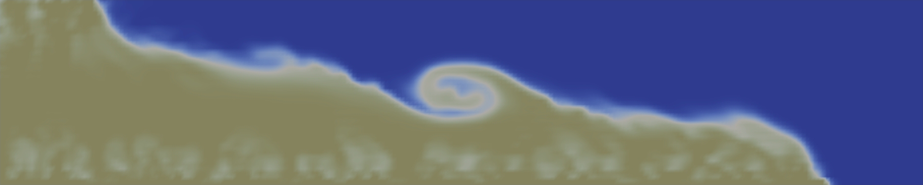
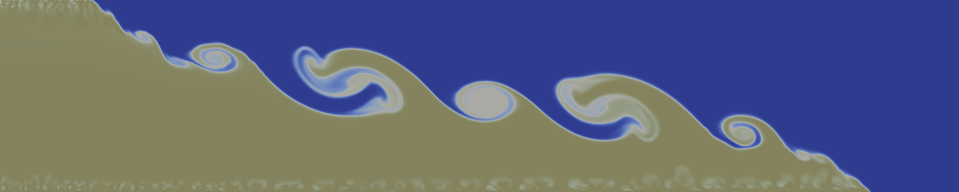
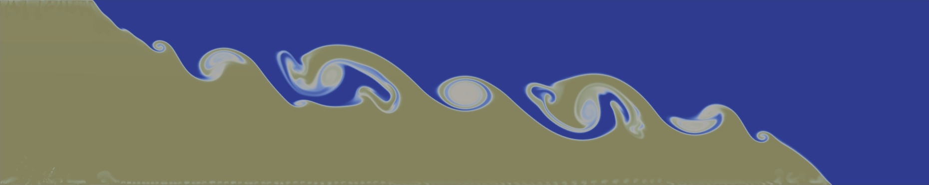
Figure 2: Snapshots of the solid-phase bulk density at $t/T_{b}=0.637$ evaluated with different resolutions, (a) low-res DNS*, (b) mid-res DNS*, (c) ultra-res DNS.

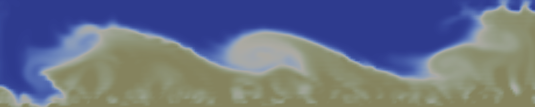
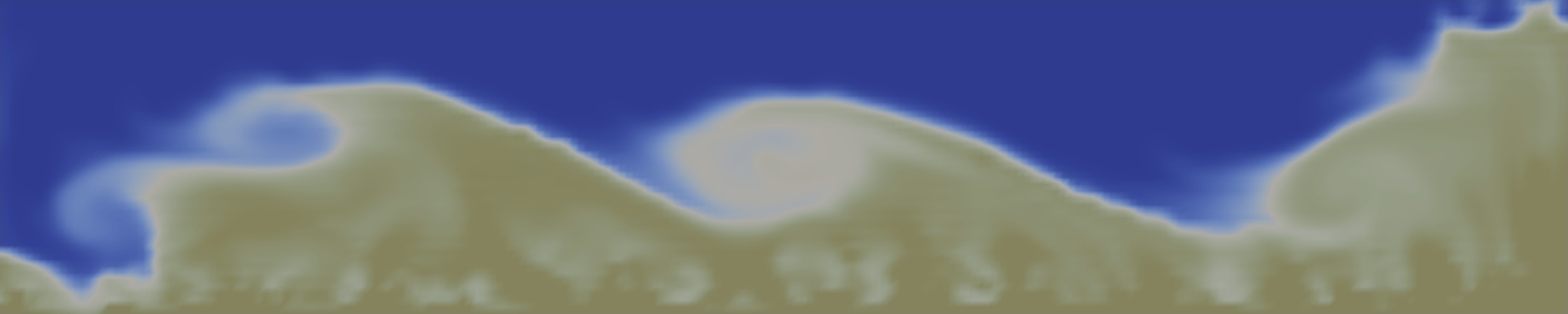
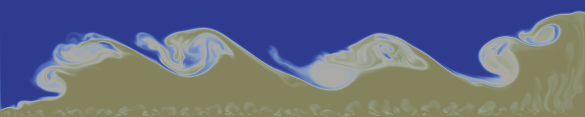
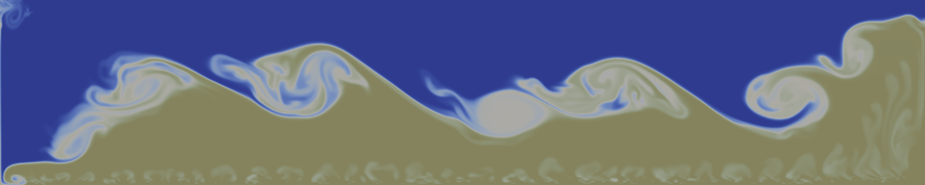
Figure 3: Snapshots of the solid-phase bulk density at $t/T_{b}=1.114$ evaluated with different LES models: (a) low-res Smagorinsky, (b) low-res one eq. eddy, (c) mid-res Smagorinsky, (d) mid-res one eq. eddy, (e) ultra-res DNS.

Figs. 1-3 show that, just as in the case of the Boussinesq equations, the system rapidly generates the Kelvin-Helmholtz billows along the interface of gravity waves, which are counter-propagating. These waves are reflected by the side walls and gradually both billows grow by entraining the surrounding fluid. Later the mixing increases so much that individual billows cannot be seen anymore.

In order to check whether our DNS results are an appropriate benchmark for the LES results, we compare our ultra-res DNS results with those in [27]. Since we chose analogous initial conditions and since our two-phase model is comparable with the Boussinesq equations (cf. Eq. (6)), we expect similar qualitative results for all the flow variables. In Fig. 4 we compare our ultra-res DNS results with those from [27]

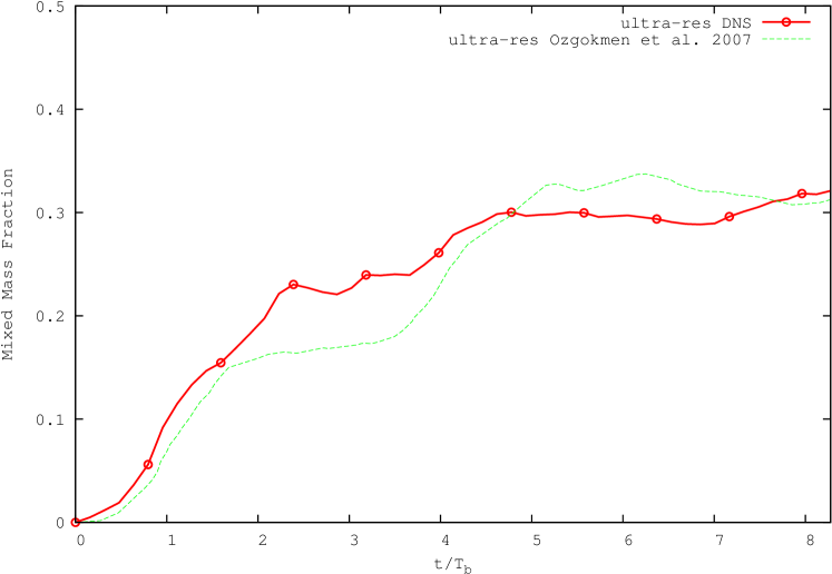
Figure 4: Time evolution of the mixed mass fraction. DNS results from the current study (solid) and from Ref [27] (dashed). Both simulations use the same mesh resolution.

using the mixed mass fraction, which is a quantity measuring the mixing. The mixed mass fraction is defined as the fraction of volume were the density perturbation is partially mixed. In particular, in our simulations with homogeneous meshes, it is obtained evaluating the percentage of cells such that $1/3<\rho_{s}<2/3$ (cf. [27]). The plots in Fig. 4 show that the two simulations yield similar results, as expected. The main difference is in the time interval $2<t/T_{b}<4$, where our simulation seems to mix slightly more than the simulation from [27]. As we will discuss later, this is probably due to the mixing induced by the creation of stratification.

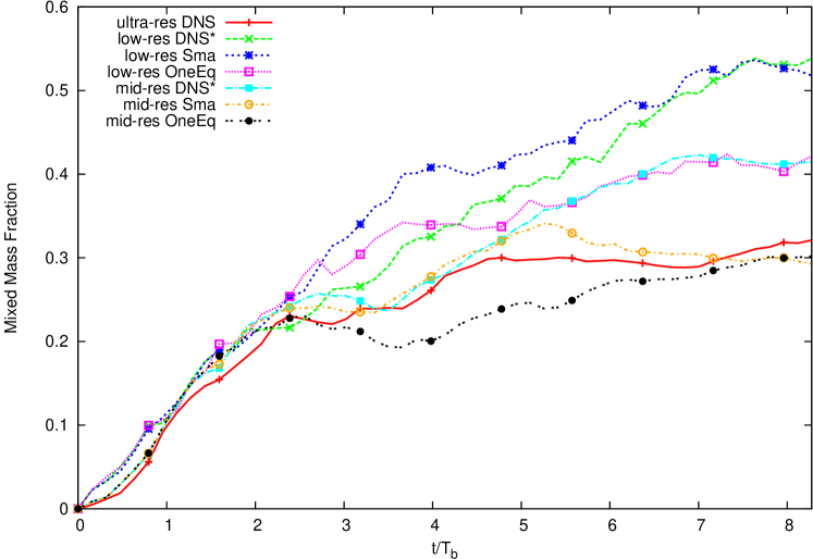
Figure 5: Time evolution of the mixed mass fraction with $\frac{1}{3}<\rho_{s}<\frac{2}{3}$ for the various low resolution LES models. The DNS results (solid) serve as benchmark.

In Fig. 5 we plot the evolution of the mixed mass fraction for all our simulations. Fig. 5 yields the following conclusions: At the low-res, the one equation eddy model performs the best, followed by the DNS*, and the Smagorinsky model (in this order). At the mid-res, the Smagorinsky model performs the best, followed by the one equation eddy model, and the DNS* (in this order).

The main measure used in the assessment of the accuracy of the models employed to predict mixing in the dam-break problem is the non-dimensional background potential energy RPE* defined in (7), cf. [32].

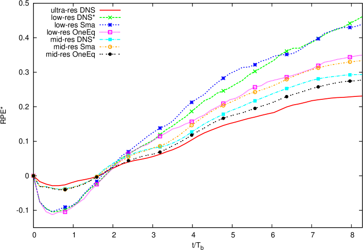
Figure 6: Time evolution of the non-dimensional background energy ($\textup{RPE}^{*}$), for the LES models at various resolutions. The DNS results (solid) serve as benchmark. The time is normalized with $T_{b}$.

Figure 6 plots the background energy of the various LES models. The DNS results serve as benchmark. Fig. 6 yields the following conclusions: At the low-res, the one equation eddy model performs the best, followed by the DNS*, and the Smagorinsky model (in this order). At the mid-res, the one equation eddy model again performs the best, followed by the DNS*, and the Smagorinsky model (in this order).

Apart from the above LES model assessment, we also observe that new important phenomena appear in the compressible case: While in the incompressible case the RPE is monotonically increasing, in our investigation it is initially decreasing, it then reaches a minimum, and it finally starts to increase monotonically, as expected. In order to better understand this phenomenon, we have to compare the background energy of the homogeneous initial condition with that of the stratified initial condition. Evaluating the initial potential energy ($\textup{PE}_{0}$), the available energy ($\textup{APE}_{0}$), and the background energy ($\textup{RPE}_{0}$) for the homogeneous initial density of the solid-phase, we get:

$$\textup{PE}_{0}/g =10, \textup{APE}_{0} =5, \textup{RPE}_{0}/g=5.$$ (8)

If we consider the initial distribution of fluid and particles in the stratified case, with $\rho_{s}(x,z,0)=0.01\,\rho_{f}(x,z,0)$, and $\rho_{f,\textup{homog.}}=100$, we get

$$\rho_{s}(x,z)=\frac{1-\eta\,z}{1-\eta\frac{H}{2}}\mathcal{H}(-x)\,,$$ (9)

where $\mathcal{H}(x)$ is the Heaviside step function. Evaluating the same energies (as those in (8)) for the stratified density distribution considered and using $H=2$ and $L=10$, we get

$$\textup{PE}_{\textup{str.}}/g =\frac{10}{3}\frac{(3-4\eta)}{1-\eta}, \textup{APE}_{\textup{str.}} =\frac{1}{2}\textup{PE}_{\textup{str.}}, \textup{RPE}_{\textup{str.}}=\frac{1}{2}\textup{PE}_{\textup{str.}}\,,$$ (10)

and also

$$\textup{RPE}_{\textup{str.}}^{*}=\frac{\textup{RPE}_{\textup{str.}}-\textup{RPE}_{0}}{\textup{RPE}_{0}}=\frac{-\eta}{3(1-\eta)}<0\,.$$ (11)

These analytical computations show that the RPE of the stratified state is smaller than that of the homogeneous state. In the next section we will discuss this issue in more detail.

3.4 A few remarks on the model without the barotropic assumption.

In this section, we compare the results of the previous sections with some low-res simulations obtained from the same test case, by using system (4), i.e. without the assumption of a barotropic fluid. The simulations with model (4) are more time-consuming and so we performed them only at low-res (simulations with finer mesh resolution are in preparation and their results will appear in the forthcoming report [5]).

The barotropic assumption is based on the fact that the thermal and kinematic diffusion ($\nabla\cdot q$ and $\mathbb{T}:\nabla u$) in Eq. (4) are negligible, so that the entropy $s$ of the system is constant along streamlines, i.e. $(\partial_{t}+u\cdot\nabla)s(x,z,t)=0$ (cf. [11] for the one-phase case and [5] for the multiphase case): This is a reversibility assumption. Indeed, the background energy can be considered as a sort of entropy, measuring the potential energy dispersed in the mixing [32]. The fact that the transformation is reversible allows the background energy to decrease. On the contrary, if we remove this assumption, coming back to the full multiphase model (4) (including the energy equation), we find that the background energy becomes monotone, see Fig. 7. This figure suggests that the barotropic assumption may be not completely justified during the initial time-interval needed to adjust from the homogeneous to the stratified condition (probably this transformation can not be considered fully iso-entropic). Nevertheless, the barotropic assumption seems justified after the time $T_{a}$.

Moreover, the stratified initial condition makes the simulation more stable and accurate, but also less diffusive, even at low-res. The RPE* is monotonically increasing when using model (4) (low-res irreversible) and, starting with the stratified initial condition, decreases the mixing and brings it closer to that of the DNS.

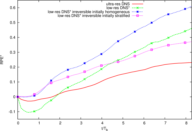
Figure 7: Plot of RPE* obtained by using model (4). Low res DNS* compared with the ultra-res DNS and the low-res DNS*. The line with “$\cdot\!\cdot\!\square\!\cdot\!\cdot$” represents RPE* starting from the initial condition (9), while the line with “- -$\ast$- -” represents the same quantity starting from the homogeneous initial state. The solid line and the line with “- -$\times$- -” are the RPE* obtained with the barotropic model (5) with homogeneous initial state, with the ultra-res DNS and the low-res DNS*, respectively.

Note that the low-res DNS* irreversible with homogeneous initial data and the ultra-res DNS start from the same datum. Even if the low-res DNS* is under-resolved, the behavior of the RPE* is correct and it is monotonically increasing. The behavior, at the beginning of the evolution, is closer to the DNS than the behavior of the LES described in Fig. 6, obtained from the barotropic model (5). On the other hand, after this transient time the behavior becomes comparable with that of the previous low-res barotropic simulation (low-res DNS* vs. low-res DNS* irreversible and homogeneous). The comparison of the results obtained at various resolutions and with different LES models for the barotropic and non-barotropic equations deserves further investigation and we plan to perform it in the near future.

4 Conclusions

We examined a two-dimensional dam-break problem were the instability is due to the presence of a dilute suspension of particles in half of the domain. The Reynolds number based on the typical gravity wave velocity and on the semi-height of the domain is $4300$, the Froude number is $2^{-\frac{1}{2}}$, the Mach number is $10^{-2}$, and the Prandtl number is $1$. The particle concentration is $10^{-3}$, and the Stokes number is smaller than $10^{-3}$ (fine particles). The importance of stratification, measured as the density gradient times the domain height ($-\partial_{y}\rho_{f}/\rho_{f}\,H$), is about a few percent ($\sim 5\%$). Even if the problem is quasi-incompressible and quasi-isothermal, we used a full compressible code, with a barotropic constitutive law. We employed a homogeneous and orthogonal mesh with three different grid refinements ranging from $10^{4}$ to $10^{6}$ cells. A posteriori tests confirm that the finer grid can resolve all the scales of the problem. The code that we used was derived from the OpenFOAM${}^{\textup{\textregistered}}$ C++ libraries.

We compared our quasi-isothermal two-phase simulations with the analogous mono-phase problem, where the mixing occurs between the same fluid at two different temperatures, as reported in [27]. As we showed in Section 2, this is possible since the two physical problems become mathematically equivalent in the regimes under study. As expected, we found a good agreement between the two sets of numerical results. We reported the evolution of the background (or reference) potential energy (RPE), a scalar quantity measuring the mixing between the two fluids. The main contributions of this report are the following: We implemented a multiphase Eulerian model (that can be used in more complex physical situations, with more than two phases, and also involving chemical reactions between species, as in volcanic eruptions). We also showed the effectiveness of the numerical results obtained programming with an open-source code. More importantly, we discovered that peculiar effects due to compressibility influence the mixing. In the literature we found that the mono-phase, incompressible Boussinesq test case has a monotonically increasing RPE. On the other hand, in our numerical experiments with slightly compressible two-phase flow, we found that the RPE initially decreases because of the stratification instability, and then it increases monotonically because of the mixing between the particles and the surrounding fluid. Indeed, even if the flow is quasi-incompressible ($\textup{Ma}=0.01$), it turns out that stratification effects are not negligible. We reported the preliminary results in the two-dimensional case. We plan to perform three-dimensional numerical simulations of the same problem in a future study.

References

- [1] S. Balachandar and J.K. Eaton. Turbulent dispersed multi-phase flow. Annu. Rev. Fluid Mech., vol. 42, pp. 399–434. Annual Reviews, Palo Alto, CA, 2010.
- [2] L.C. Berselli, P. Fischer, T. Iliescu, and T. Özgökmen. Horizontal Large Eddy Simulation of stratified mixing in a lock-exchange system. J. Sci. Comput., 49:3–20, 2011.
- [3] R. E. Britter and J.E. Simpson. Experiments on the dynamics of a gravity current head. J. Fluid Mech., 88:223–240, 1978.
- [4] G.F. Carrier. Shock waves in a dusty gas. J. Fluid Mech, 4:376–382, 1958.
- [5] M. Cerminara. Multiphase flows in volcanology. PhD thesis, Scuola Normale Superiore, 2014. To appear.
- [6] M. Cerminara, L.C. Berselli, T. Esposti Ongaro, and M.V. Salvetti. Direct numerical simulation of a compressible multiphase flow through the eulerian approach. In Direct and Large-Eddy Simulation IX, vol. 12 of ERCOFTAC Series. Springer, 2013. At press.
- [7] T. Chacón Rebollo and R. Lewandowski. Mathematical and numerical foundations of turbulence models and applications. Birkhäuser, Boston, 2014.
- [8] B. Cushman-Roisin and J.-M. Beckers. Introduction to Geophysical Fluid Dynamics. Academic Press, 2nd edition, 2011. ISBN: 978-0-12-088759-0.
- [9] Ä. Dörnbrack. Turbulent mixing by breaking gravity waves. J. Fluid Mech. 375:113–141, 1998.
- [10] T. Esposti Ongaro, C. Cavazzoni, G. Erbacci, A. Neri, and M.V. Salvetti. A parallel multiphase flow code for the 3d simulation of explosive volcanic eruptions. Parallel Comput., 33(7-8):541–560, 2007.
- [11] E. Feireisl. Dynamics of viscous compressible fluids, Oxford University Press, Oxford, 2004.
- [12] H.J.S. Fernando. Aspects of stratified turbulence. In: Kerr, R.M., Kimura, Y. (Eds.), Developments in Geophysical Turbulence, pp. 81–92, 2000.
- [13] J.H. Ferziger and M. Perić. Computational methods for fluid dynamics, revised ed., Springer-Verlag, Berlin, 1999.
- [14] U. Frisch. Turbulence, The Legacy of A.N. Kolmogorov. Cambridge University Press, Cambridge, 1995.
- [15] C. Fureby. On subgrid scale modeling in large eddy simulations of compressible fluid flow. Phys. Fluids, 8(5):1301–1311, 1996.
- [16] J. Hacker, P. F. Linden, and S. B. Dalziel. Mixing in lock-release gravity currents. Dyn. Atmos. Oceans, 24(1-4):183–195, 1996.
- [17] M.A. Hallworth, H.E. Huppert, J.C. Phillips, and R.S.J. Sparks. Entrainment into two-dimensional and axisymmetric turbulent gravity currents. J. Fluid Mech., 308:289–311, 1996.
- [18] M.A. Hallworth, J.C. Phillips, H.E. Huppert, and R.S.J. Sparks. Entrainment in turbulent gravity currents. Nature, 362:829 – 831, 1993.
- [19] R.I. Issa. Solution of the implicitly discretised fluid flow equations by operator-splitting. J. Comput. Phys., 62(1):40–65, 1986.
- [20] H. Jasak. Error Analysis and Estimation for the Finite Volume Method with Applications to Fluid Flows. PhD thesis, Imperial College, London, 1996.
- [21] L.H. Kantha and C.A. Clayson. Small Scale Processes in Geophysical Fluid Flows, vol. 67 of Int. Geophysics Series. Academic Press, 2000.
- [22] D.A. Kay, P.M. Gresho, D.F. Griffiths, and D.J. Silvester. Adaptive time-stepping for incompressible flow. II. Navier-Stokes equations. SIAM J. Sci. Comput., 32(1):111–128, 2010.
- [23] F. Marble. Dynamics of dusty gases. Annu. Rev. Fluid Mech., vol. 3, pp. 397–446. Annual Reviews, Palo Alto, CA, 1970.
- [24] B. R. Morton, G. Taylor, and J.S. Turner. Turbulent gravitational convection from maintained and instantaneous sources. Proc. R. Soc. Lond. A, 234, 1–23 1956.
- [25] T. Özgökmen, T. Iliescu, and P. Fischer. Large eddy simulation of stratified mixing in a three-dimensional lock-exchange system. Ocean Modelling, 26:134–155, 2009.
- [26] T. Özgökmen, T. Iliescu, and P. Fischer. Reynolds number dependence of mixing in a lock-exchange system from direct numerical and large eddy simulations. Ocean Modelling, 30(2):190–206, 2009.
- [27] T. Özgökmen, T. Iliescu, P. Fischer, A. Srinivasan, and J. Duan. Large eddy simulation of stratified mixing in two-dimensional dam-break problem in a rectangular enclosed domain. Ocean Modelling, 16:106–140, 2007.
- [28] J.J. Riley and M.-P. Lelong. Fluid motions in presence of strong stable stratification. In Annu. Rev. Fluid Mech., vol. 32, pp. 613–657. Annual Reviews, Palo Alto, CA, 2000.
- [29] D.A. Siegel and J.A. Domaradzki. Large-eddy simulation of decaying stably stratified turbulence. J. Phys. Oceanogr., 24:2353–2386, 1994.
- [30] Y.J. Suzuki, T. Koyaguchi, M. Ogawa, and I. Hachisu. A numerical study of turbulent mixing in eruption clouds using a 3D fluid dynamics model. J. Geophys. Res.: Solid Earth, 110(B8):B08201, 2005.
- [31] S.A. Valade, A.J.L. Harris and M. Cerminara. Plume Ascent Tracker: Interactive Matlab software for analysis of ascending plumes in image data. Comput. & Geosci., 66(0):132–144, 2014.
- [32] K.B. Winters, P.N. Lombard, J.J. Riley, and E.A. D’Asaro. Available potential energy and mixing in density-stratified fluids. J. Fluid Mech., 289:115–128, 4 1995.