Optical Response of Sr₂RuO₄ Reveals Universal Fermi-liquid Scaling
and Quasiparticles Beyond Landau Theory

Abstract

We report optical measurements demonstrating that the low-energy relaxation rate ($1/\tau$) of the conduction electrons in Sr₂RuO₄ obeys scaling relations for its frequency ($\omega$) and temperature ($T$) dependence in accordance with Fermi-liquid theory. In the thermal relaxation regime, $1/\tau\propto(\hbar\omega)^{2}+(p\pi k_{\mathrm{B}}T)^{2}$ with $p=2$, and $\omega/T$ scaling applies. Many-body electronic structure calculations using dynamical mean-field theory confirm the low-energy Fermi-liquid scaling, and provide quantitative understanding of the deviations from Fermi-liquid behavior at higher energy and temperature. The excess optical spectral weight in this regime provides evidence for strongly dispersing “resilient” quasiparticle excitations above the Fermi energy.

Liquids of interacting fermions yield a number of different emergent states of quantum matter. The strong correlations between their constituent particles pose a formidable theoretical challenge. It is therefore remarkable that a simple description of low-energy excitations of fermionic quantum liquids could be established early on by Landau Landau (1956), in terms of a dilute gas of “quasiparticles” with a renormalized effective mass, of which ³He is the best documented caseBaym and Pethick (2004); Leggett (2004).

Breakdown of the quasiparticle concept can be observed in the transport of metals tuned onto a quantum phase transition, but Fermi-liquid (FL) behavior is retrieved away from the quantum-critical region Sachdev (1998); Čubrović et al. (2009). The relevance of FL theory to electrons in solids is documented by a number of materials, such as transition metals Rice (1968), heavy-fermion compounds Kadowaki and Woods (1986), and doped semiconductors van der Marel et al. (2011). Among transition-metal oxides, Sr₂RuO₄ is a remarkable example which has been heralded as the solid-state analogue of ³He Mackenzie and Maeno (2003) for at least three reasons: remarkably large and clean monocrystalline samples can be prepared, transport properties display low-temperature FL characteristics Hussey et al. (1998), and there is evidence for $p$-wave symmetry of its superconducting phase Kallin (2012), as in superfluid ³He.

FL theory makes a specific prediction for the universal energy and temperature dependence of the inelastic lifetime of quasiparticles: Because of phase-space constraints imposed by the Pauli principle as well as momentum and energy conservation, it diverges as $1/\omega^{2}$ or $1/T^{2}$ Landau (1956); Čubrović et al. (2009). More precisely, the inelastic optical relaxation rate is predicted to vanish according to the scaling law $1/\tau\propto(\hbar\omega)^{2}+(p\pi k_{\mathrm{B}}T)^{2}$, with $p=2$ Gurzhi (1959); Maslov and Chubukov (2012); Berthod et al. (2013). This leads to universal $\omega/T$ scaling of the optical conductivity $\sigma(\omega)$ in the thermal regime $\hbar\omega\sim k_{\mathrm{B}}T$ Berthod et al. (2013). Surprisingly however, despite almost 60 years of research on Fermi liquids, this universal behavior of the optical response, and especially the specific statistical factor $p=2$ relating the energy and temperature dependence have not yet been established experimentally Basov et al. (2011); Maslov and Chubukov (2012); Berthod et al. (2013); Nagel et al. (2012); Mirzaei et al. (2013).

Here, we report optical measurements of Sr₂RuO₄ with 0.1 meV resolution Kidd et al. (2005); Ingle et al. (2005) which reveal this universal FL scaling law . We establish experimentally the universal value ${p~{}=~{}2}$ and demonstrate remarkable agreement between the experimental data and the theoretically derived scaling functions in the FL regime. Importantly, the identification of the precise FL response also enables us to characterize the deviations from FL theory. The manifestation of these deviations in our data is an excess spectral weight above $0.1$ eV. We show that this is an optical fingerprint of the abrupt increase in dispersion of “resilient” quasiparticle excitations. This confirms the recent prediction Deng et al. (2013) on the basis of dynamical mean-field theory (DMFT), that well-identified peaks in the spectral function persist far above the asymptotic low-energy and low-temperature Landau FL regime where the relaxation rate has a strict $\omega^{2}$ dependence. In this Letter, we perform realistic DMFT calculations for Sr₂RuO₄ which yield excellent agreement with the measured optical spectra. There are three bands at $E_{F}$: a two-dimensional one ($\gamma$) of $d_{xy}$ character and two quasi-1D bands ($\alpha$ and $\beta$), respectivelyMackenzie and Maeno (2003). We show that the deviations from FL behavior in the optical spectra are caused by resilient quasiparticle (QP) excitations associated with unoccupied states, which are inaccessible in usual photoemission experiments.

Optical spectroscopy is a powerful probe of—among other things—the subtle low-energy behavior of electron liquids. Earlier optical studies of Sr₂RuO₄ have reported that the in-plane low-energy spectral weight is about 100 times larger than the one along the $c$ axis, with an onset below 25 K of a $T^{2}$ relaxation rate Katsufuji et al. (1996); Hildebrand et al. (2001); Pucher et al. (2003). The lowest-lying interband transitions, located above 1 eV, have been previously identified as $d$-$d$ transitions Lee et al. (2002). In the optical conductivity of Sr₂RuO₄ this is revealed as a peak at 1.7 eV (SM , Table I). In the range displayed in Fig. 1, $\sigma(\omega)$ is entirely due to the free carrier response. The dynamical character of the inelastic scattering can be captured by a frequency-dependent memory function $M(\omega)$ as described in Ref. Götze and Wölfle, 1972 so that

$$\sigma(\omega)=\frac{i\epsilon_{0}\omega_{p}^{2}}{\omega+M(\omega)}.$$ (1)

On the other hand, an intraband optical absorption process excites electron-hole pairs, with the consequence that the optical relaxation rate $M_{2}(\omega)$ is proportional to $(\hbar\omega)^{2}+(p\pi k_{\mathrm{B}}T)^{2}$ with the value $p=2$ Gurzhi (1959); Maslov and Chubukov (2012); Berthod et al. (2013). The optical conductivity is then characterized by a narrow Lorentzian-like zero-frequency mode (Drude peak), followed by a (non-Drude) “foot” at $\hbar\omega\approx 2\pi k_{\mathrm{B}}T$ Berthod et al. (2013). Hence, the signature of FL theory and of the frequency dependence of $1/\tau$ is actually a deviation from Drude’s form (corresponding to a constant $\tau$).

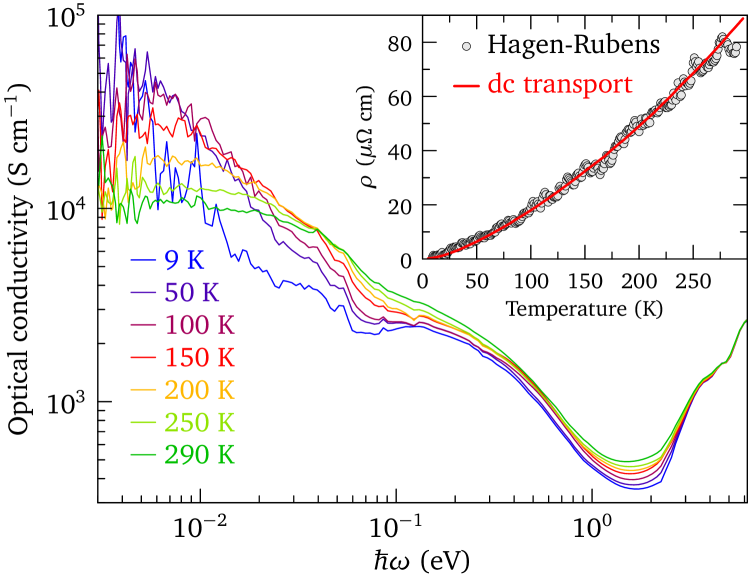
Figure 1: Real part of the optical conductivity of Sr₂RuO₄ for selected temperatures between 9 and 290 K. Inset: Zero-frequency resistivity determined by the Hagen-Rubens fit of the reflectivity (open circles) and four-terminal dc resistivity of the same crystal (solid red curve) multiplied with a factor 0.84, which is within the range of geometrical factors due to sample shape and contact layout.

Several recent optical studies have reported $\omega^{2}$ and $T^{2}$ for $M_{2}(\omega)$ in a number of different materials. However, in neither of these cases does the coefficient $p$ match the prediction $p=2$: $p\sim 1$ in URu₂Si₂ Nagel et al. (2012), $p\sim 2.4$ in the organic material BEDT-TTF Dressel (2011), and $p\sim 1.5$ in underdoped HgBa₂CuO_4+δ Mirzaei et al. (2013). One possible scenario that has been proposed to explain this discrepancy is the presence of magnetic impurities Maslov and Chubukov (2012). We decided instead to look at the $4d$ correlated material Sr₂RuO₄which can be synthesized in very pure form, with well-established $T^{2}$ resistivity below 25 K Mackenzie and Maeno (2003).

The Sr₂RuO₄ crystal employed for this work was grown by sing the travelling floating zone technique Udagawa et al. (2005). The quality of the crystal was confirmed by different techniques Fittipaldi et al. (2005) with a superconducting transition at 1.4 K. The $ab$-plane crystal surface of $5.1\times 3.6$ mm² was micropolished and cleaned prior to transferring the sample to the UHV cryostats for optical spectroscopy. Near-normal reflection reflectivity spectra in the range from 2 meV to 3 eV were collected between 290 and 9 K at a cooling rate of 1 K per minute. The optical conductivity obtained by Kramers-Kronig analysis is shown in Fig. 1 for a few selected temperatures. The close match of the dc resistivity and $\rho(T)=\mbox{lim}_{\omega\rightarrow 0}1/\sigma_{1}(\omega,T)$ (inset in Fig. 1) provides evidence that the low-frequency optical data are accurate at all temperatures.

The optical conductivity displayed in Fig. 1 is dominated by the peak centered at zero frequency, corresponding to the optical response of the free charge carriers. Upon lowering the temperature from 290 to 9 K this peak becomes extremely narrow, and its maximum at $\omega=0$ increases by 2 orders of magnitude. The weak features at 40, 57, and 85 meV correspond to optical phonons. The standard Drude model assumes a frequency-independent relaxation rate. The frequency dependence of $M_{2}(\omega)$ shown in Fig. 2(b) is therefore manifestly non-Drude like, and signals the presence of a dynamical component in the quasiparticle self-energy. Moreover, below 0.1 eV, $M_{2}(\omega)$ has a positive curvature for all temperatures corresponding to $\omega^{\eta}$ with $\eta\approx 2$ (SM , Sec. III), and $M_{1}(\omega)$ has a linear frequency dependence that is only weakly changing with temperature. This is the expected behavior in a Fermi liquid. The low-frequency mass enhancement factor $m^{*}(\omega)/m=1+M_{1}(\omega)/\omega$ varies from 3.3 at 9 K to 2.3 at 290 K. The $m^{*}(\omega)/m$ curves (SM , Sec. II) fall slightly below the one of a previous room temperature study Lee et al. (2006).

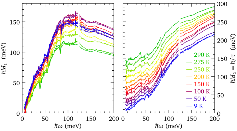
Figure 2: Real part (left) and imaginary part (right) of the Sr₂RuO₄ memory function for selected temperatures between 9 and 290 K. A white space is introduced near 130 meV where data sets from different detectors were linked.

In order to reveal the signature of Fermi-liquid behavior, we searched for the presence of a universal scaling of the form $M_{2}(\omega,T)\propto\xi_{p}^{2}\equiv(\hbar\omega)^{2}+(p\pi k_{\mathrm{B}}T)^{2}$ in the data, by plotting $M_{2}(\omega,T)$ parametrically as a function of $\xi_{p}^{2}$ for different choices of $p$ and calculating the root-mean square (rms) deviation of this plot from a straight line. The frequency range used in this analysis was limited to $\hbar\omega\leq 36~{}\mathrm{meV}$, and the largest temperature considered, $T_{\max}$, was allowed to vary down to $T_{\max}=35$ K, below which the fitted temperature range becomes too small to produce reliable output. The result of the scaling collapse for $p=2$ and $T\leq T_{\max}=40$ K is displayed in Fig. 3. The rms minimum for each $T_{\max}$ defines $p^{*}$, shown as a function of $T_{\max}$ in the inset. When the range $T_{\max}$ is varied from 100 to 35 K we observe a flow from $p=1.5$ towards the plateau value $p=2$, which is approached for $T_{\max}\leq 50$. This confirms the expectation of a flow towards universal Fermi-liquid behavior for $T\rightarrow 0$, for which we expect a collapse of all data on a universal function of $\xi_{p}$ with $p=2$. A similar analysis conducted on the raw reflectivity data leads to the same conclusion that $p=2$(SM , Sec. III).

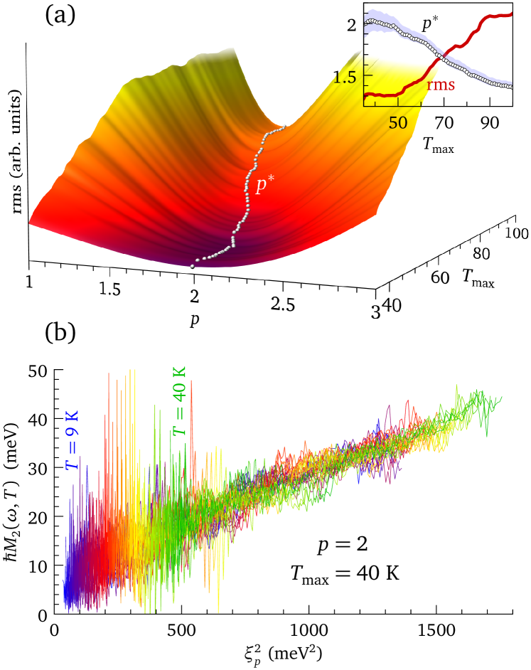
Figure 3: (a) Root-mean square deviation of the relaxation rate $M_{2}(\omega,T)$ from a linear dependence in $\xi_{p}^{2}$, for $\hbar\omega\leq 36~{}\mathrm{meV}$ and $T\leq T_{\max}$, as a function of $p$ and $T_{\max}$. The inset shows the value $p^{*}$ and the rms at the minimum versus $T_{\max}$. A value $p^{*}=2$ is found below $T_{\max}\sim 40$ K. The shaded region shows how $p^{*}$ changes if the frequency range is varied by $\pm 5$ meV. (b) Collapse of the relaxation rate data for $T\leq 40$ K.

A direct confirmation of FL behavior is found in the optical conductivity curves (Fig. 4). They exhibit a characteristic non-Drude feature in perfect agreement with the universal FL response. This feature is an increase of conductivity with respect to the low-frequency Drude response around the thermal frequency $\hbar\omega=2\pi k_{\mathrm{B}}T$, appearing most clearly as a shoulder in a log-log plot. The universal FL response, including impurity scattering, has been parametrized by only three temperature-independent parameters Berthod et al. (2013). This three-parameter model can reproduce the low-frequency optical conductivity data of Sr₂RuO₄ in the whole temperature range below 40 K, where $p=2$, as illustrated in Fig. 4.

For energies above 0.1 eV and/or temperatures above 40 K, the measured conductivities clearly depart from the reference FL (Fig. 4). All deviations go in the direction of a larger conductivity (both real and imaginary parts), in particular, in the 0.1–0.5 eV energy range. In order to understand the origin of this increased conductivity, we have calculated the optical spectra within an ab initio framework that combines density-functional theory (DFT) with the many-body DMFT Georges et al. (1996), as described in Aichhorn et al. (2009); Ferrero et al. and applied to Sr₂RuO₄ in Mravlje et al. (2011). The bare dispersions and velocities are obtained from DFT for the three $t_{2g}$ bands, and the local (momentum-independent) DMFT self-energies for each orbital are calculated by using the same interaction parameters as in previous works (SM , Sec. IV). The theoretical results are presented in Fig. 4 as circles. The overall shapes of experimental data and theoretical DMFT results match closely, and satisfactory agreement is also found for absolute values (note that the comparison in Fig 4 involves no scale adjustment). At low frequency and temperature, the ab initio calculations show a Drude peak and a thermal shoulder, in excellent agreement with the experimental data and with the FL model. The differences at the lowest frequencies can be attributed to impurity scattering, included in the FL model but not in the DMFT calculation, in order to keep the latter parameter-free. More interestingly, above 0.1 eV the theory deviates from the FL model in precisely the same manner as the experiment does. At higher temperatures, while the predictions extrapolated from the low-temperature FL severely underestimate the conductivity, the agreement between DFT+DMFT and experiments remains excellent in the 0.1–0.5 eV range.

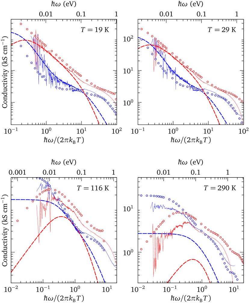
Figure 4: Comparison of the experimental optical conductivity (solid lines), Fermi-liquid model (dashed lines), and DFT+DMFT calculation (circles) at selected temperatures. The real and imaginary parts of the conductivity are shown in blue and red, respectively. The three parameters of the Fermi-liquid model, including impurity scattering, are fit to the experimental data in the range $\hbar\omega\leq 36~{}\mathrm{meV}$ and $T\leq 40$ K. The DFT+DMFT calculation ignores impurity scattering.

The calculated imaginary part of the optical conductivity is systematically somewhat lower than the experimental data. The difference increases with temperature, and is most clear for 290 K. Electron-phonon interactions in fact cause additional mass-enhancement, which leads to a suppression of both $\sigma_{1}$ and $\sigma_{2}$ for $\omega\rightarrow 0$ and an increase of optical conductivity in the phonon energy range. This effect is not included in the DMFT calculations and may explain the remaining differences with experimental data.

We have carried out a series of numerical experiments in order to elucidate the origin of the non-FL excess of optical spectral weight in the $0.1$–$0.5$ eV frequency range (SM , Sec. IV). First, we eliminated band-structure effects as a possible cause. The band structure enters the optical conductivity via a transport function $\Phi(\varepsilon)$, proportional to the average of the squared velocities at a given energy. This function is smooth, unlike the density of states which diverges at the van Hove singularity of the $xy$ band. Indeed, we have verified that the replacement of $\Phi(\varepsilon)$ by its Fermi-surface value $\Phi(0)$ causes no significant change in the theoretical curves of Fig. 4. The excess spectral weight is therefore due to electronic correlations and must be linked to a structure in the single-particle self-energies.

The imaginary part of the self-energies follows the FL parabolic dependence at low-energy but starts to deviate already well below 0.1 eV in the direction of a weaker scattering. In particular, between $+0.2$ and $+0.4$ eV, still in the domain of intraband transitions, the scattering rate goes through a maximum and decreases slightly at higher energy. A similar phenomenon with a saturation of the scattering rate was observed in the single-band Hubbard model and was shown to give rise to resilient QPs Deng et al. (2013). In Sr₂RuO₄, the signature of resilient QPs is even more striking: It is signaled by a drop of the scattering rate for empty states above $\sim 0.35$ eV. Consistently with Kramers-Kronig relations, this drop implies a sharp minimum in the real part of the self-energy which is found in the energy range 0.1–0.15 eV. As a consequence, QPs above this energy scale have velocities larger than the bare velocities. In the theoretical spectral function, these appear as peaks which are broader than the low-energy Landau QP peaks and have a very steep dispersion in the range 0.2–0.4 eV, leading to an inverted waterfall-like structure.

These resilient QPs with large velocities are the source of excess spectral weight and deviation from FL behavior above 0.1 eV. Indeed, optical spectroscopy is sensitive to these excitations above the Fermi level since it probes transitions between occupied and unoccupied states. The abrupt increase of QP velocities predicted by DFT+DMFT results in a maximum in the real part of the calculated memory function $M_{1}(\omega)$ in the range 0.1–0.2 eV, hence providing an explanation for the corresponding feature found experimentally (Fig. 2). We also note that more subtle changes in QP dispersions (kinks) at $\sim 30$ meV, previously found in both angle-resolved photoemission spectroscopy (ARPES) Ingle et al. (2005); Iwasawa et al. (2013) and DMFT Mravlje et al. (2011), are also visible in $M_{1}$ and $M_{2}$ at lower energy but do not change the frequency dependence of the optical conductivity so strikingly.

The resilient QP excitations above the Fermi level predicted by our calculations and leading to the sharp feature in $M_{1}$ are not directly accessible to conventional ARPES, which probes only occupied states. Recently, two-photon ARPES has been shown to provide energy and momentum-resolved information on unoccupied states Sobota et al. (2013), and we propose that our theoretical results (SM , Fig. SM14) could be put to the test in the future by using this technique for Sr₂RuO₄.

In summary, we have performed reflectance and ellipsometry measurements for a Sr₂RuO₄ single crystal in a wide range of frequencies and temperatures and observed for the first time the universal optical signatures of the Landau quasiparticles in a FL. The low-energy optical relaxation rate obeys $(\hbar\omega)^{2}+(p\pi k_{\mathrm{B}}T)^{2}$ scaling with $p=2$, and the optical conductivity exhibits a pronounced non-Drude foot at the thermal frequency $\hbar\omega=2\pi k_{\mathrm{B}}T$. The identification of a low-energy FL regime provides a reference to characterize without ambiguity the deviations from FL theory. In Sr₂RuO₄, the most significant deviation at low temperature is an increase of conductivity developing above $0.1$ eV. With the help of DFT+DMFT calculations, we ascribed the extra spectral weight to resilient quasiparticle excitations above the Fermi level, i.e., relatively broad but still strongly dispersing particlelike excitations with a lifetime differing from the Landau low-energy form. This work demonstrates that optical spectroscopy is a powerful tool to diagnose non-FL behavior, with the provision that the proper FL behavior is taken as the “placebo” reference, instead of the Drude law that is often used for that purpose.

I Optical spectroscopy

The measurement of the in-plane optical response was carried out with two FTIR spectrometers and a Woolam VASE ellipsometer. The far-infrared to near-infrared reflectivity at near-normal incidence was measured from 1.9 meV to 1.1 eV (15 to 9000 cm^-1) using a Bruker 113 FTIR spectrometer. A Bruker 66 upgraded with a high-frequency module extended this range to 3 eV. The ellipsometry measurements were performed in a Woolam VASE ellipsometer, completing and extending the data up to the UV (0.47–6.2 eV). The two spectroscopic techniques thus overlap from 0.47 to 3 eV. Light polarized along the $a\!b$ plane (p-polarization) was used in order to suppress the $c$-axis features, as described in Ref. van Heumen et al., 2007.

We used Sr₂RuO₄ crystals containing less than 2 volume percent intercalated layers of Sr₃Ru₂O₇ of three unit cell thickness on average. The crystals show no detectable trace of the 3K phase. The crystal was cleaved along the $a\!b$ plane, polished to achieve a perfectly reflective surface, and glued onto a copper sample holder using silver paste. The device was mounted in a high vacuum and high stability home-made cryostat ($\sim 10^{-8}$ mbar) including an in-situ gold/silver evaporator to cover the sample with a reference layer. Temperature sweeps were conducted between 9 K and 290 K at a speed of 1 K per minute, and one reflectivity spectrum was collected every Kelvin. The long-term drift of the light sources and detectors was calibrated using a high stability flipping mirror placed in front of the cryostat window. The mirror was flipped up and down every 20 minutes, providing a continuous monitoring of the signal drift. The remaining uncorrected drift was analyzed during the warmup process, which leads to a thermal hysteresis effect below the noise level in the far IR, below 0.2% in the mid IR, and below 0.4% in the near IR and above.

The calibrated $a\!b$-plane reflectivity is obtained as

$$R(\omega)=\frac{I_{\mathrm{sample}}(\omega)}{I_{\mathrm{reference}}(\omega)}\frac{I_{\mathrm{reference-mirror}}(\omega)}{I_{\mathrm{sample-mirror}}(\omega)},$$ (2)

where $I_{\mathrm{sample-mirror}}(\omega)$ and $I_{\mathrm{reference-mirror}}(\omega)$ are the intensities from the mirror, measured together with the sample and reference, respectively. The absolute reflectivity $R(\omega)$ is shown for selected temperatures in Fig. SM1. The figure also shows the room-temperature $c$-axis reflectivity reproduced from Ref. Katsufuji et al., 1996.

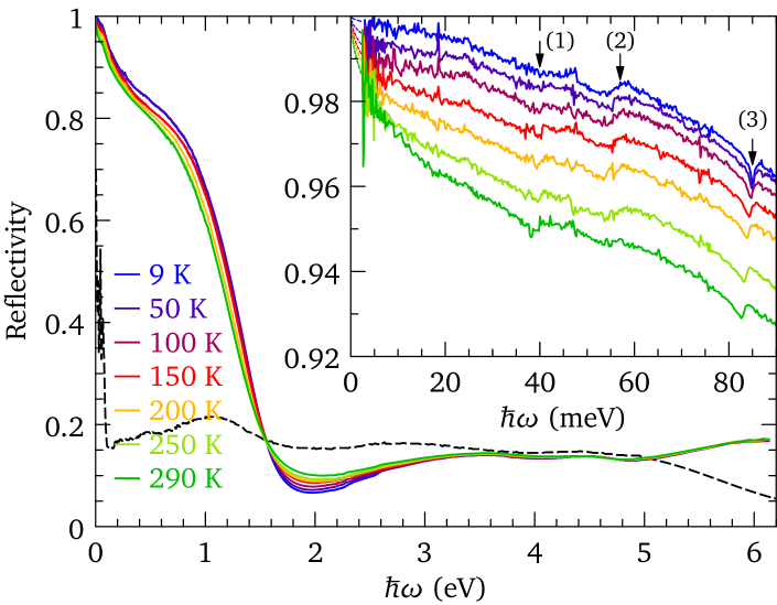
Figure SM1: Optical reflectivity of Sr₂RuO₄ along the $a\!b$ plane (solid lines) and $c$ axis (dashed line, reproduced from Ref. Katsufuji et al., 1996) at selected temperatures. The inset shows the low-frequency region, with the Hagen-Rubens extrapolation to zero frequency, Eq. (5), shown as dashed lines. The 84 meV feature (3) is a longitudinal in-plane bond-stretching phonon mode of the RuO₂ layer (zone center double degenerated E_u). The slight softening and broadening upon heating indicate a decrease of screening. The structures (1) at 40 meV and (2) at 57 meV most likely also correspond to phonons.

The ellipsometry data is used to extend the frequency range up to 6.2 eV. The angle of incidence $\theta$ of the light was 70^∘ measured from the surface normal. Owing to the anisotropy of Sr₂RuO₄, the measured complex dielectric function $\tilde{\epsilon}(\omega)$ (the so-called pseudo-dielectric function) is a mix of the $a\!b$-plane and $c$-axis responses. The $a\!b$-plane dielectric function $\epsilon(\omega)=\epsilon_{1}(\omega)+i\epsilon_{2}(\omega)$ was extracted from $\tilde{\epsilon}(\omega)$ by inverting the Fresnel equations, using the complex $c$-axis dielectric function $\epsilon_{c}(\omega)$ deduced from the $c$-axis reflectivity of Ref. Katsufuji et al., 1996:

$$\tilde{\epsilon}=\sin^{2}\!\theta+\sin^{4}\!\theta\\ \times\left(\frac{\sqrt{\epsilon-\sin^{2}\!\theta}\sqrt{\epsilon^{\phantom{2}}}-\sqrt{1-\epsilon_{c}^{-1}\sin^{2}\!\theta}}{\sqrt{\epsilon-\sin^{2}\!\theta}\sqrt{1-\epsilon_{c}^{-1}\sin^{2}\!\theta}-\sqrt{\epsilon^{\phantom{2}}}\cos^{2}\!\theta}\right)^{2}.$$ (3)

The resulting $\epsilon(\omega)$ is shown in Fig. SM2. Following Ref. van Heumen et al., 2007, the consistency of the procedure for extracting $\epsilon(\omega)$ has been checked by repeating the ellipsometry measurements at several angles of incidence.

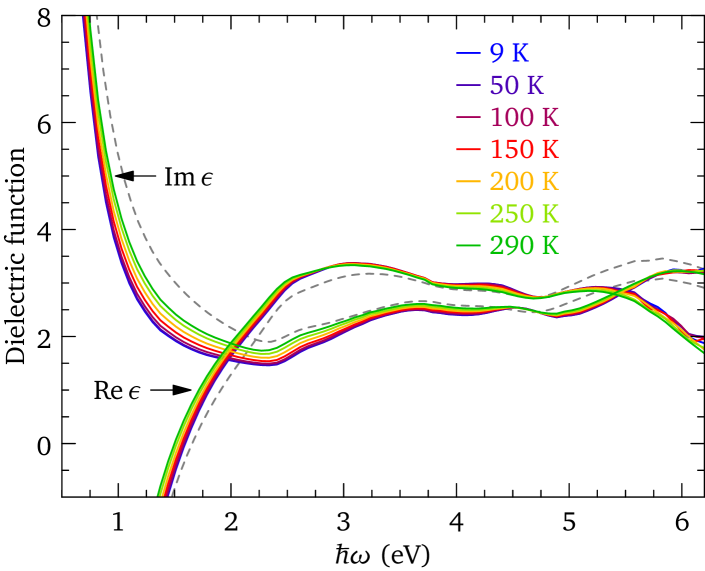
Figure SM2: Real and imaginary parts of the dielectric function $\epsilon$ extracted from Eq. (3). The dashed lines show the complex pseudo dielectric function $\tilde{\epsilon}$ at 290 K.

A Kramers-Kronig transform of the reflectivity, using the ellipsometry data to anchor the phase, provides the complex optical conductivity $\sigma(\omega)=\sigma_{1}(\omega)+i\sigma_{2}(\omega)$. The dielectric function and the conductivity are related by $\epsilon(\omega)=1+i\sigma(\omega)/(\epsilon_{0}\omega)$. The reflection coefficient is given by

$$R(\omega)=\left|\frac{1-\sqrt{\epsilon(\omega)}}{1+\sqrt{\epsilon(\omega)}}\right|^{2}\approx 1-4\mathrm{Re}\,\sqrt{\frac{1}{\epsilon(\omega)}}.$$ (4)

The right-hand side of this expression applies to the infrared frequency range, where $|\epsilon(\omega)|\gg 1$. Furthermore for $\omega\ll 1/\tau$ the conductivity can be approximated by $\sigma_{1}(\omega)=1/\rho$, where $\rho$ is the dc resistivity. Eq. (4) then becomes the Hagen-Rubens relation Hagen and Rubens (1903)

$$R(\omega)\approx 1-\sqrt{{8\epsilon_{0}\omega\rho}}.$$ (5)

A fit of this formula to the low-frequency reflectivity, shown in the inset of Fig. SM1 as dashed lines, yields the temperature-dependent resistivity $\rho(T)$ shown in Fig. 1 of the main text.

II Drude-Lorentz analysis, memory function

The in-plane reflectivity and ellipsometry data are fitted simultaneously using the standard Drude-Lorentz model. The low-energy response below $\sim 1$ eV is well described at all temperatures by the superposition of two Drude (zero-frequency) oscillators. Above 1 eV, the data are fitted with four additional Lorentz oscillators. The high-frequency limit is represented by the constant $\epsilon_{\infty}$, leading to the following model for $\epsilon(\omega)$:

$$\epsilon(\omega)=\epsilon_{\infty}+\sum_{j=1}^{6}\frac{\omega_{pj}^{2}}{\omega_{j}^{2}-\omega(\omega+i\gamma_{j})}.$$ (6)

The parameters of the model fitted to the room-temperature data are given in Table 1. The real part of the conductivity calculated using this model is displayed in Fig. SM3, and compared with the conductivity determined directly by Kramers-Kronig transform of the reflectivity. The match is excellent up to 5.8 eV.

Table 1: Parameters of the Drude-Lorentz oscillators for the in-plane optical response of Sr₂RuO₄ at 290 K. All numbers are in eV. The high-frequency dielectric constant is $\epsilon_{\infty}=2.3$. The intraband plasma frequency obtained from the two Drude oscillators is $\hbar\omega_{p}=3.4$ eV.

$j$	1	2	3	4	5	6
$\hbar\omega_{j}$	0.000	0.000	1.693	3.730	4.489	6.298
$\hbar\gamma_{j}$	0.038	0.432	1.952	2.533	0.602	2.527
$\hbar\omega_{pj}$	1.568	3.014	1.552	4.123	0.843	6.826

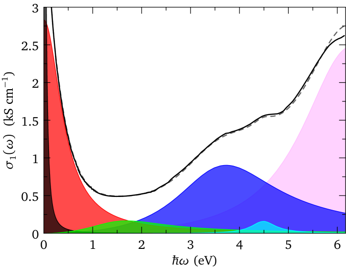
Figure SM3: Real part of the optical conductivity at 290 K, calculated from the Drude-Lorentz model given by Eq. (6) and Table 1 (dashed line). The shaded curves show the contributions of the six oscillators, with the two Drude oscillators in black and red. The solid line is the conductivity obtained directly from the reflectivity and ellipsometry data using Kramers-Kronig relations.

The Drude-Lorentz analysis allows us to distinguish the contribution of the mobile charge carriers from that of the bound charges. At all temperatures considered, the analysis yields two zero-frequency modes, as well as finite-energy contributions that are all above 1 eV. The two Drude modes mimic the “foot” structure of the low-energy Fermi-liquid response described in the main text. We ascribe the two Drude oscillators to the intraband response of mobile carriers, and all finite-energy modes to the bound charges. The spectral weight of the charge carriers is, in units of $\epsilon_{0}$,

$$\omega_{p}^{2}\equiv\sum_{\hbar\omega_{j}=0}\omega_{pj}^{2}.$$ (7)

This gives a spectral weight that is almost temperature independent, corresponding to $\hbar\omega_{p}=3.3$ eV at low temperature and 3.4 eV at room temperature. Note that the spectral weight of the sharpest Drude mode is smaller, and decreases from $\hbar\omega_{p1}=1.8$ eV at low temperature to 1.6 eV at room temperature.

In the energy range $\hbar\omega<1$ eV of interest for the present study, the interband transitions do not contribute to the frequency dependence of the dielectric function, as can be seen in Fig. SM4. The bound-charge dielectric function defined as

$$\epsilon_{\mathrm{bound}}(\omega) =\epsilon_{\infty}+\sum_{\hbar\omega_{j}>0}\frac{\omega_{pj}^{2}}{\omega_{j}^{2}-\omega(\omega+i\gamma_{j})}$$ (8)

$$\approx\epsilon_{\infty}+\sum_{\hbar\omega_{j}>0}\frac{\omega_{pj}^{2}}{\omega_{j}^{2}}$$ (9)

is practically constant over this energy range, and equal at 290 K to $\epsilon_{\mathrm{bound}}(0)=5.6$.

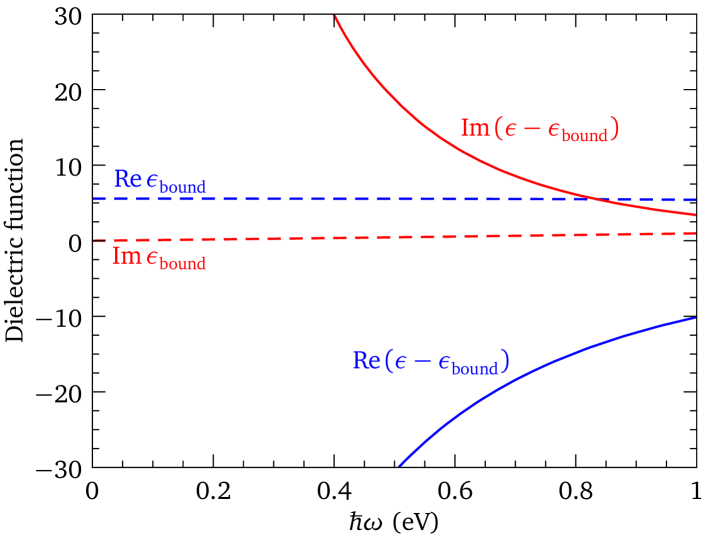
Figure SM4: Mobile- and bound-charge contributions to the dielectric function at 290 K. The negligible frequency dependence of the bound-charge response indicates a clear separation between the intraband and interband responses below 1 eV.

Knowing the intraband spectral weight $\epsilon_{0}\omega_{p}^{2}$, we may invert Eq. (1) of the main text, and express the memory function, or optical self-energy $M(\omega)=M_{1}(\omega)+iM_{2}(\omega)$, in terms of the optical conductivity:

$$1+\frac{M_{1}(\omega)}{\omega} \equiv\frac{m^{*}(\omega)}{m}=\mathrm{Im}\,\left[\frac{-\epsilon_{0}\omega_{p}^{2}}{\omega\sigma(\omega)}\right]$$ (10)

$$M_{2}(\omega) \equiv\frac{1}{\tau(\omega)}=\mathrm{Re}\,\left[\frac{\epsilon_{0}\omega_{p}^{2}}{\sigma(\omega)}\right].$$ (11)

The memory function is displayed for selected temperatures in Fig. 2 of the main text, and the mass enhancement factor in Fig. SM5. It presents an overall behavior determined by the charge-carrier dynamics, as well as sharp superimposed Fano-like structures corresponding to dipole active optical phonons. We do not subtract phonons, which would require a specific modeling and introduce unwanted ambiguities.

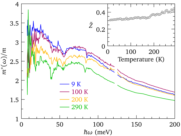
Figure SM5: Frequency-dependent mass enhancement $m^{*}(\omega)/m=1+M_{1}(\omega)/\omega$ for some selected temperatures, and temperature dependence of $\tilde{Z}=m/m^{*}(\omega)$ extrapolated to zero frequency. The white space close to 130 meV indicates the region where two data sets have been linked.

III Fermi-liquid analysis

The universal characteristics of the optical response in a Fermi liquid have been described in Ref. Berthod et al., 2013. For a local Fermi liquid, i.e., with a momentum-independent self-energy, the low-energy optical conductivity normalized to the dc conductivity is a universal function of the two variables $\hbar\omega/(2\pi k_{\mathrm{B}}T)$ and $\omega\tau_{\text{qp}}$, where $\tau_{\text{qp}}$ is the quasiparticle life-time on the Fermi surface. This life-time diverges as $1/T^{2}$ with decreasing temperature in a Fermi liquid. In Ref. Berthod et al., 2013, it was parametrized by a temperature scale $T_{0}$, such that $\hbar/\tau_{\text{qp}}$ equals $2\pi k_{\mathrm{B}}T$ at this temperature: $\hbar/\tau_{\text{qp}}=2\pi(k_{\mathrm{B}}T)^{2}/(k_{\mathrm{B}}T_{0})$. The parameter $T_{0}$ completely determines the universal behavior of $\sigma(\omega)/\sigma_{\text{dc}}$. The non-universal dc conductivity depends on the quasiparticle residue $Z$, and on the transport function $\Phi(0)$ proportional to the average squared velocity on the Fermi surface. In the dc conductivity, these two quantities enter as the product $Z\Phi(0)$. This product also coincides with the weight of the Drude peak. The Fermi-liquid model can be generalized to include impurity scattering in the form of a constant scattering rate $\Gamma$, entering the optical conductivity as the product $Z\Gamma$. Thus the low-energy optical conductivity of a local Fermi liquid can be represented by the three parameters $T_{0}$, $Z\Phi(0)$, and $Z\Gamma$. The temperature scale $T_{0}$ is a relatively large scale, typically ten times larger than the scale $T_{\mathrm{FL}}$, below which the universal Fermi-liquid behavior is generally observed Berthod et al. (2013).

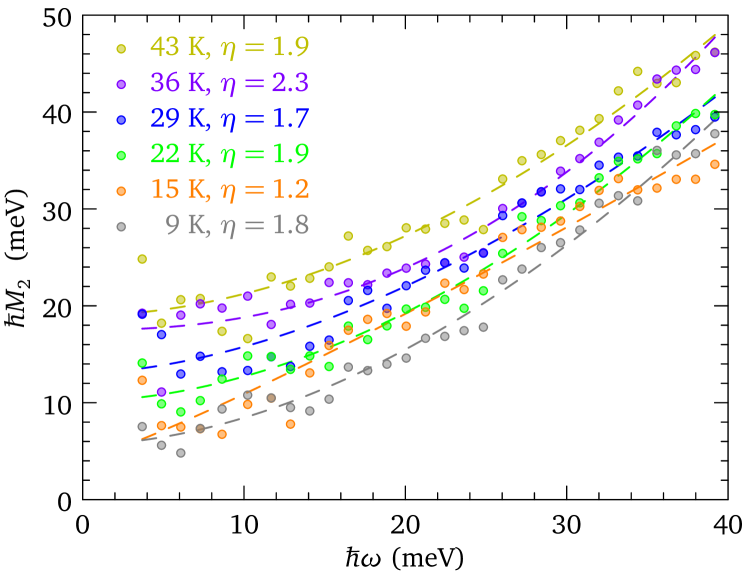
Figure SM6: Imaginary part of the memory function binned in 2 meV intervals (points) for selected temperatures. The data is fitted below 40 meV using the power law $M_{2}(\omega)=M_{2}(0)+A\omega^{\eta}$ (dashed lines). The exponent $\eta$ is indicated for each temperature.

In the present study, the experimental intraband response is represented by the complex memory function $M=M_{1}+iM_{2}$, $\sigma(\omega)=i\epsilon_{0}\omega_{p}^{2}/[\omega+M(\omega)]$, and the reference spectral weight $\epsilon_{0}\omega_{p}^{2}$ is taken as the intraband weight, determined as explained in Sec. II. In the thermal regime, $\hbar\omega\sim 2\pi k_{\mathrm{B}}T$, the Fermi-liquid memory function has the form

$$M(\omega)\approx\left(\frac{1}{\tilde{Z}}-1\right)\omega\\ +\frac{2i}{\hbar\tilde{Z}}\left(\frac{(\hbar\omega)^{2}+(2\pi k_{\mathrm{B}}T)^{2}}{3\pi k_{\mathrm{B}}T_{0}}+Z\Gamma\right).$$ (12)

$\tilde{Z}=Z\Phi(0)/(\epsilon_{0}\omega_{p}^{2})$ is the ratio of the Drude weight to the reference weight. In the Fermi-liquid regime, a plot of $\hbar M_{2}$ as a function of $\xi^{2}=(\hbar\omega)^{2}+(2\pi k_{\mathrm{B}}T)^{2}$ yields a straight line with a slope $2/(3\pi k_{\mathrm{B}}T_{0}\tilde{Z})$, and an intercept $2Z\Gamma/\tilde{Z}$. For Sr₂RuO₄, this scaling behavior is observed for temperatures below $\sim 40$ K and frequencies below $\sim 36$ meV, as shown in Fig. 3 of the main text. Fitting $M_{2}(\omega)$ using a power law in that frequency and temperature range (Fig. SM6) indicates a clear curvature $\omega^{\eta}$ with $\eta=1.7$–$2.3$, with one outlier ($T=15$ K), where the least-squares fit gives $\eta=1.15$.

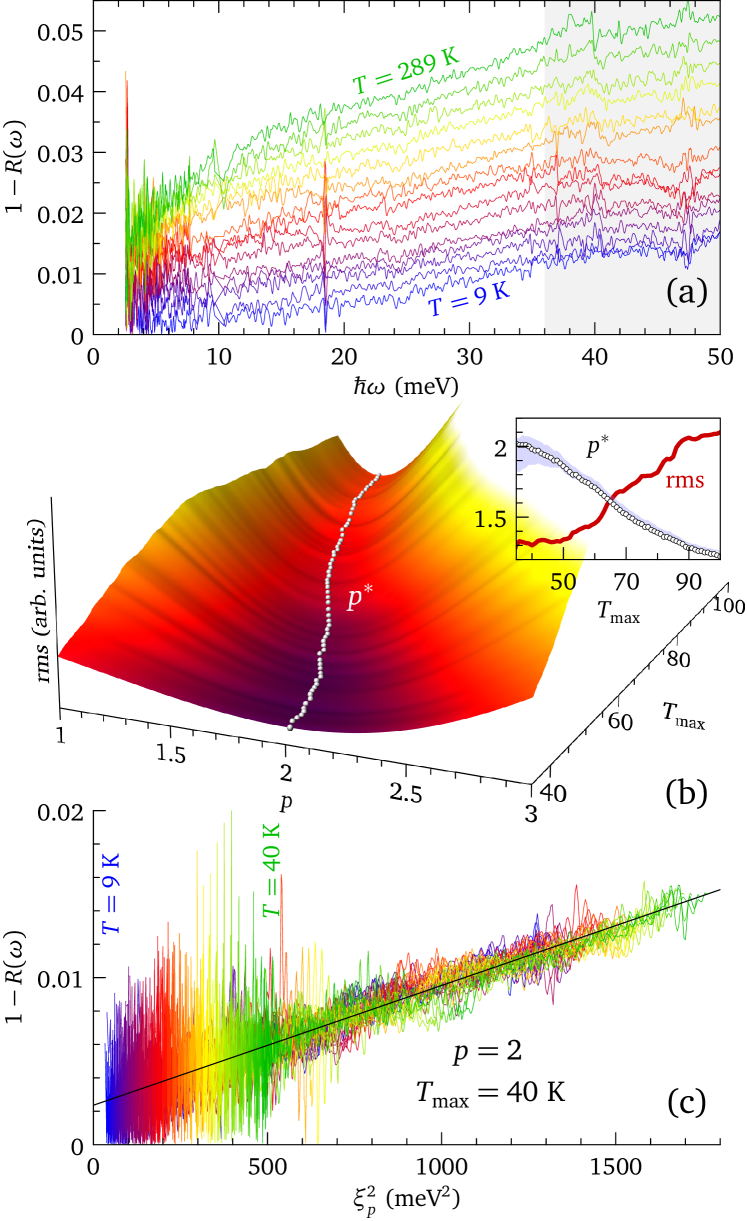
Figure SM7: (a) Reflectivity data plotted as $1-R(\omega)$ versus $\hbar\omega$ for $9~{}\text{K}\leqslant T\leqslant 290$ K (one curve every 20 K). The data in the shaded region ($\hbar\omega>36$ meV) is ignored in the Fermi-liquid scaling analysis. (b) Root-mean square deviation of the reflectivity for $T\leqslant T_{\max}$ from a linear dependence in $\xi_{p}^{2}$, as a function of $p$ and $T_{\max}$. The inset shows the value $p^{*}$ (dots) and the rms (solid, arbitrary units) at the minimum, versus $T_{\max}$. The shaded region shows how $p^{*}$ changes if the range of frequencies retained in the analysis is varied by $\pm 5$ meV. (c) Collapse of the reflectivity data for $T\leqslant 40$ K. Blue corresponds to $T=9$ K and green to $T=40$ K. The linear correlation coefficient is 0.9.

The frequency and temperature scaling properties of the optical relaxation rate in the thermal regime, $\hbar\omega\sim 2\pi k_{\mathrm{B}}T$, can also be observed in the bare reflectivity data at normal incidence. We substitute the definition of the memory function in Eq. (4), and expand in powers of $M_{2}/(\omega+M_{1})$:

$$1-R(\omega)\approx\sqrt{\frac{8\epsilon_{0}\omega}{Z\Phi(0)}\left(M_{2}+\sqrt{(\omega+M_{1})^{2}+M_{2}^{2}}\right)}=\\ 2\sqrt{\frac{\epsilon_{0}}{Z\Phi(0)}}\frac{M_{2}}{\omega+M_{1}}+O\left(\left[\frac{M_{2}}{\omega+M_{1}}\right]^{2}\right).$$ (13)

Substituting Eq. (12) for $M(\omega)$ we find that, in the thermal regime, $1-R(\omega)$ behaves like $M_{2}(\omega)$:

$$1-R(\omega)=\frac{4}{\hbar}\sqrt{\frac{\epsilon_{0}}{Z\Phi(0)}}\left[\frac{(\hbar\omega)^{2}+(2\pi k_{\mathrm{B}}T)^{2}}{3\pi k_{\mathrm{B}}T_{0}}+Z\Gamma\right].$$ (14)

In order to test the presence of this scaling in the Sr₂RuO₄ reflectivity, we proceed like for the imaginary part of the memory function in the main text: for all temperatures $T\leqslant T_{\max}$ and all frequencies $\hbar\omega\leqslant 36$ meV, we plot $1-R(\omega)$ as a function of $\xi_{p}^{2}=(\hbar\omega)^{2}+(p\pi k_{\mathrm{B}}T)^{2}$, and we determine the value of $p$ which minimizes the rms deviation of the data from a straight line. The result of this analysis is shown in Fig. SM7. It leads to the same conclusion as the analysis performed on the memory function: the Fermi-liquid universal behavior with $p=2$ is only seen below $T\sim 40$ K. We note that the optimal value of $p$ depends to some extent on the window of frequencies considered. Extending the window up and down by 5 meV leads to changes in the curve $p^{*}(T_{\max})$ as indicated in the inset of Fig. SM7(b). With the reflectivity data, which is not affected by uncertainties of the Kramers-Kronig transform, the curve is less sensitive to the frequency window than with the memory-function data of Fig. 3 in the main text.

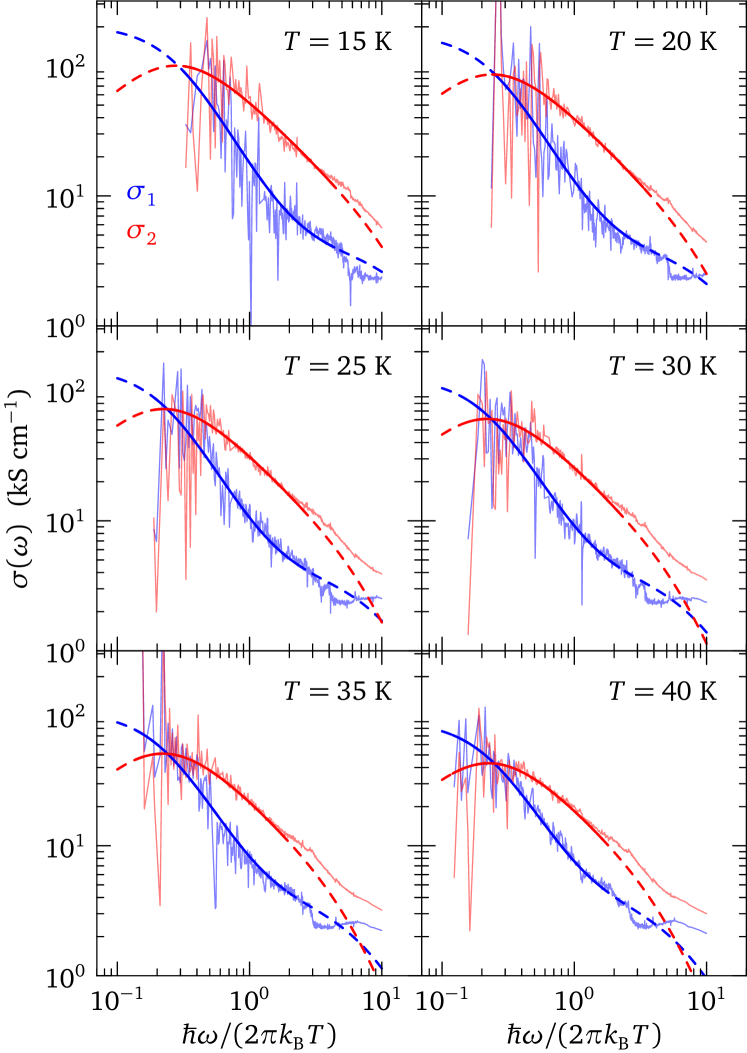
Figure SM8: Optical conductivity of Sr₂RuO₄ in the Fermi-liquid regime. The thin lines show the real ($\sigma_{1}$, blue) and imaginary parts ($\sigma_{2}$, red) of the measured conductivity. The thick lines show the fit to the Fermi-liquid model of Ref. Berthod et al., 2013, with the parameters $T_{0}=316$ K, $\hbar^{2}Z\Phi(0)=3.5\epsilon_{0}\text{eV}^{2}$, and $Z\Gamma=0.9$ meV. The lines are solid in the frequency range below $\hbar\omega\leqslant 36~{}\text{meV}$ considered for the fit, and dashed outside this range.

In the frequency and temperature domain where the above analysis points to Fermi-liquid behavior with $p=2$, the real and imaginary parts of the Sr₂RuO₄ optical conductivity display a characteristic change of curvature around $\hbar\omega=2\pi k_{\mathrm{B}}T$. This can be seen in Fig. SM8: the low-frequency Drude behavior of $\sigma_{1}$ changes to a weaker frequency dependence for $\hbar\omega>2\pi k_{\mathrm{B}}T$. A similar change of slope was identified in Ref. Berthod et al., 2013 to be a signature of the universal Fermi-liquid response. Adjusting the local-Fermi liquid model to the data in the domain $\hbar\omega\leqslant 36~{}\text{meV}$ and $T\leqslant 40$ K, we find that it provides a very good fit of the measured conductivity (see Fig. SM8). This should be regarded as an effective one-band description of the three-band response of Sr₂RuO₄. The effective model parameters resulting from the fit are $T_{0}=316$ K, $\hbar^{2}Z\Phi(0)=3.5\epsilon_{0}\text{eV}^{2}$, and $Z\Gamma=0.9$ meV. The Drude weight $Z\Phi(0)$ corresponds to a plasma frequency $\approx 1.87$ eV, in good agreement with the value of $\hbar\omega_{p1}$ obtained from the Drude-Lorentz analysis at $T=9$ K (Sec. II).

IV Ab initio calculations

IV.1 Method

We calculated the optical conductivity within an ab-initio framework that combines density-functional theory (DFT) in the local-density approximation (LDA) as implemented in Wien2k Blaha et al. (2001), with the many-body dynamical mean-field theory (DMFT) Georges et al. (1996). The framework is described in Ref. Aichhorn et al., 2009.

The optical conductivity in DFT+DMFT is expressed as

$$\sigma(\omega)=\frac{2\pi e^{2}}{V}\sum_{\bm{k}}\int_{-\infty}^{\infty}d\varepsilon\,\frac{f(\varepsilon)-f(\varepsilon+\hbar\omega)}{\omega}\\ \times\mathrm{Tr}\,v_{\bm{k}}^{x}A_{\bm{k}}^{\phantom{x}}(\varepsilon)v_{\bm{k}}^{x}A_{\bm{k}}^{\phantom{x}}(\varepsilon+\hbar\omega).$$ (15)

$V$ is a normalization volume, $f(\varepsilon)$ is the Fermi function, $\bm{v}_{\bm{k}}$ and $A_{\bm{k}}(\varepsilon)$ are the band velocities and the spectral functions, respectively, both evaluated at wave-vector $\bm{k}$. $v_{\bm{k}}^{x}$ and $A_{\bm{k}}$ are matrices in the band indices. The velocities are obtained from DFT as described in Refs. Ambrosch-Draxl and Sofo, 2006; Blaha et al., 2001, and the spectral functions are calculated as described in a previous work Aichhorn et al. (2009); Mravlje et al. (2011), using the same interaction parameters.

IV.2 Insignificance of the band velocities for the intraband conductivity

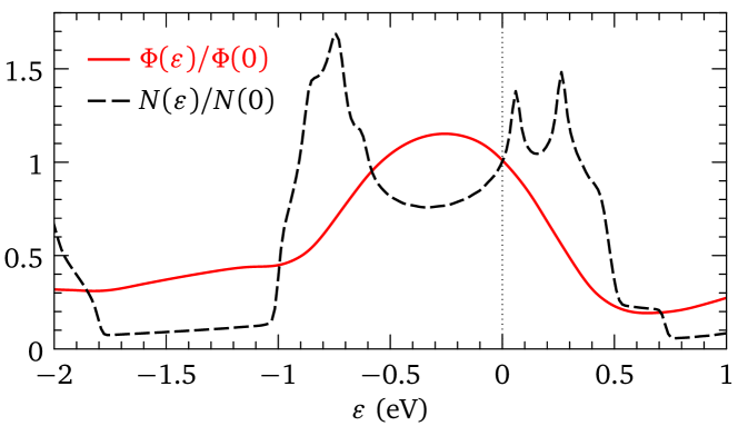
Figure SM9: Sr₂RuO₄ in-plane transport function $\Phi(\varepsilon)$, and DOS $N(\varepsilon)$, normalized to their Fermi-level values. $\Phi(0)=\epsilon_{0}\omega_{p}^{2}=0.38\times 10^{21}~{}(\Omega\mathrm{ms})^{-1}$ ($\hbar\omega_{p}=4.3$ eV), in reasonable agreement with previous results Oguchi (1995); Singh (1995).

We first address the question whether the increase of optical conductivity reported in the main text for energies above 0.1 eV, with respect to the universal Fermi-liquid (FL) behavior, could be a consequence of the bare electronic dispersions. The possible effects of the band structure must be considered, because the density of states (DOS) of Sr₂RuO₄ has a rich structure at low energy, in particular, a Van Hove singularity about 70 meV above the Fermi level (see Fig. SM9). The quantity that is relevant for the optical properties is not the DOS, though, but the transport function

$$\Phi(\varepsilon)=\frac{2e^{2}}{V}\sum_{\bm{k}}\mathrm{Tr}\,\left(v_{\bm{k}}^{x}v_{\bm{k}}^{x}\right)\,\delta(\varepsilon-\varepsilon_{\bm{k}}).$$ (16)

As can be seen in Fig. SM9, the transport function is much more smooth than the DOS, and presents no significant feature at the energy of the Van Hove singularity. This can be understood, since the band velocity vanishes at the Van Hove points.

The absence of structure in $\Phi(\varepsilon)$ suggests that the excess conductivity above 0.1 eV is not due to the band structure. To be more quantitative, we have constructed a simplified spectral function, taking for all orbitals the FL self-energy Ansatz Berthod et al. (2013)

$$\Sigma(\varepsilon)=\left(1-\frac{1}{Z}\right)\varepsilon-\frac{i}{Z\pi k_{\mathrm{B}}T_{0}}\left[\varepsilon^{2}+(\pi k_{\mathrm{B}}T)^{2}\right],$$ (17)

instead of $\Sigma_{\bm{k}}(\varepsilon)$. We used parameters that fit the self-energy of the xy band at low energy for $T=29$ K, namely, $1/Z=5.12$ and $T_{0}=400$ K. This model reproduces the universal FL result if $\Phi(\varepsilon)$ is approximated by $\Phi(0)$. In Fig. SM10, we compare the real part of the conductivity obtained using the full $\varepsilon$-dependence of $\Phi(\varepsilon)$ and the FL result. The energy dependence of the transport function does produce a deviation from the FL curve, but in the direction of a smaller conductivity, which is opposite to the experimentally observed deviation.

Figure SM10: Role of the energy dependence of the transport function $\Phi(\varepsilon)$. The solid line is the real part of the conductivity obtained by using the same Fermi-liquid self-energy, Eq. (17), for the three $t_{2g}$ bands. The dashed line is the universal FL result, where the energy dependence of $\Phi(\varepsilon)$ is neglected.

IV.3 DFT+DMFT self-energies

The local DMFT self-energies for the xy and xz/yz orbitals are shown in Fig. SM11. At low energy, both follow the FL behavior, with a parabolic dependence of the imaginary part and a linear dependence of the real part. As discussed earlier Mravlje et al. (2011), the xy orbital is more correlated, with steeper real part and stronger curvature of the imaginary part. The self-energies start to deviate from strict FL behavior already at low energy ($\sim 0.03$ eV), and become markedly electron-hole asymmetric. As seen more clearly in the real part, differences with FL dependence become substantial above 0.05 eV, especially on the electron side, where a drastic change of slope is observed.

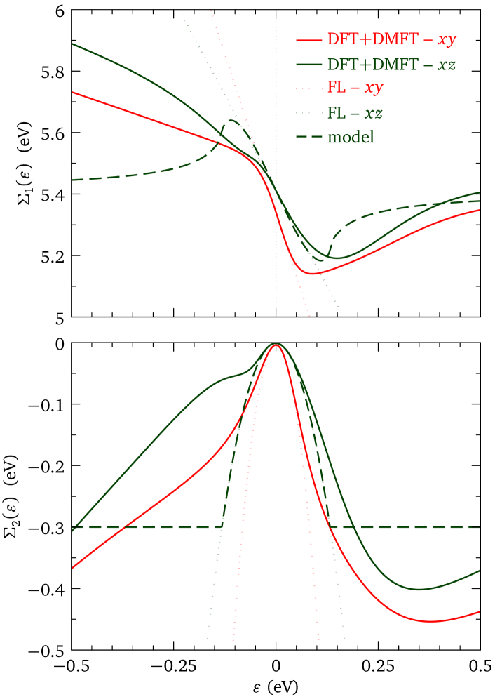
Figure SM11: Local self-energies for the xy and xz bands at $T=$ 29 K. The real part (top) is linear at low energy, and the imaginary part (bottom) is quadratic, as shown by the dotted lines. The dashed lines show a model with bounded quadratic imaginary part, and the corresponding real part.

Fig. SM11 also displays a simple model for the self-energy, with an imaginary part which is purely quadratic up to a cutoff frequency $\varepsilon_{c}=0.125$ eV, and constant with a value $\gamma_{c}=-0.3$ eV above this cutoff. The corresponding real-part, displayed in Fig. SM11, is obtained by Kramers-Kronig as:

$$\mathrm{Re}\,\Sigma(\varepsilon)=\frac{\gamma_{c}}{\pi}\left(\frac{\varepsilon^{2}}{\varepsilon_{c}^{2}}-1\right)\ln\left|\frac{\varepsilon-\varepsilon_{c}}{\varepsilon+\varepsilon_{c}}\right|+\frac{2\gamma_{c}}{\pi}\frac{\varepsilon}{\varepsilon_{c}}.$$ (18)

This model reproduces the main qualitative aspects of the data, especially the strong feature in the real part.

IV.4 Analysis of the optical response

In order to clarify the origin of the optical conductivity departure from the FL prediction above 0.1 eV, we have performed several numerical experiments. First, it is convenient to look separately at the contribution of each orbital to the conductivity. We have done this in two ways: (i) we have evaluated Eq. (15) using spectral functions in which one of the orbital was heavily damped, by adding a very large imaginary part to its self-energy; (ii) we have calculated the optical conductivity using the Allen formula Allen (2004)

$$\sigma(\omega)=\frac{i\Phi(0)}{\omega}\int_{-\infty}^{\infty}d\varepsilon\,\frac{f(\varepsilon)-f(\varepsilon+\hbar\omega)}{\hbar\omega+\Sigma^{*}(\varepsilon)-\Sigma(\varepsilon+\hbar\omega)}$$ (19)

and the local self-energy of each band independently. The results are displayed in Fig. SM12(a) and (b). For both orbitals, a deviation from FL is seen above 0.05–0.1 eV, in the direction of an increased conductivity. One also sees that the Allen formula describes the data reasonably well.

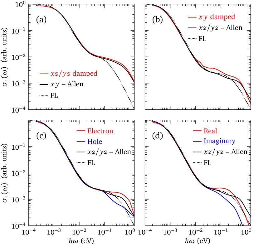
Figure SM12: (a) Optical conductivity obtained from Eq. (15), after suppressing the contributions of the $xz/yz$ orbitals (red), compared with the result of Allen formula (19) evaluated with the self-energy of the xy orbital (black), and with the universal FL curve (dotted). (b) Same as (a), with the roles of xy and $xz/yz$ exchanged. (c) Contribution of the $xz/yz$ orbitals (xy damped), with modified self-energies having either electron, or hole character (see text). (d) Contribution of the $xz/yz$ orbitals (xy damped), with modified self-energies having DMFT real part and FL imaginary part (Real) or FL real part, and DMFT imaginary part (Imaginary).

Next, we investigated which of the electron or hole part of the self-energy plays the key role in the extra conductivity. For this purpose, we defined particle-like orbital self-energies $\Sigma_{p}(\varepsilon)$, whose dependence at negative energy is obtained by the reflection of the positive-energy dependence. For the imaginary part, $\Sigma_{p2}(\varepsilon)=\Sigma_{2}(|\varepsilon|)$, and for the real part, $\Sigma_{p1}(\varepsilon<0)=2\Sigma_{1}(0)-\Sigma_{1}(-\varepsilon)$, $\Sigma_{p1}(\varepsilon>0)=\Sigma_{1}(\varepsilon)$. Similarly, hole-like self-energies are constructed by a reflection of the negative-energy data to positive energy. The resulting optical conductivities (contribution of the $xz/yz$ orbitals) are presented in Fig. SM12(c), from which it is evident that the electrons (particle-like states of positive energy), rather than the holes, give rise to the extra spectral weight.

Lastly, we investigated whether the extra conductivity must be ascribed to the real, or to the imaginary part of the self-energy. For this purpose, we constructed trial self-energies, by replacing the real or imaginary part of the DMFT self-energies with their low-energy FL extrapolations (in strong violation of Kramers-Kronig relations). The result is shown in Fig. SM12(d). One sees that keeping just the DMFT imaginary parts leads to a pronounced downward deviation from the FL result. Only when the nonlinear real parts are included does a deviation in the upward direction appear. This deviation, however, quickly dies off with such trial self-energies that violate the Kramers-Kronig relations. The reason is the rapid increase of scattering, as the FL result has already entered the dissipative regime, where increasing $|\Sigma_{2}|$ diminishes the conductivity.

The deviation from FL dependence can be reproduced qualitatively by means of the model self-energy shown in Fig. SM11. This self-energy has a quadratic imaginary part at low energy, $-\Sigma_{2}(\varepsilon)\propto\varepsilon^{2}+(\pi k_{\mathrm{B}}T)^{2}$ for $|\varepsilon|<\varepsilon_{c}$, followed by a saturation for $|\varepsilon|>\varepsilon_{c}$. The real part obtained by Kramers-Kronig displays sharp kinks at $\varepsilon_{c}$. As shown in Fig. SM13, this very rough model reproduces the data quite well. The description can be improved if the parabolic dependence of the imaginary part is kept at negative frequencies and saturation is only imposed on the positive side.

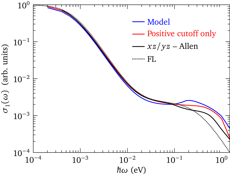
Figure SM13: Optical conductivities calculated using the Allen formula (19) with the model self-energy of Fig. SM11 (blue), and the self-energy of the $xz/yz$ orbitals (black), compared with the FL result (dotted). The red curve is obtained by sending the negative-energy cutoff of the model self-energy to $-\infty$.

IV.5 Physical interpretation: the resilient quasiparticles

The essence of the departure from the FL form is thus related to the sharp saturation of the scattering rate on the positive energy side, and the related sharp feature in the real part at a scale of 0.1 eV. The pronounced action takes place on the electron (positive energy) side. The saturation of the scattering rate and the associated robust dispersing resilient quasiparticle excitations were found in the context of the Hubbard model Deng et al. (2013). Strikingly, in Sr₂RuO₄ this saturation occurs in a more pronounced way and leads to a strong change of slope of the real part of the self-energy.

The consequences of this change of slope can be most directly seen in the color-map of the $\bm{k}$-resolved spectral function, that is presented in Fig. SM14. Superimposed are

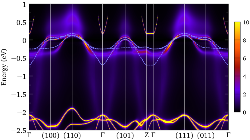
Figure SM14: Color map of the $\bm{k}$-resolved spectral function. The LDA $t_{2g}$ bands renormalized by a factor of 4 are shown with dashed lines.

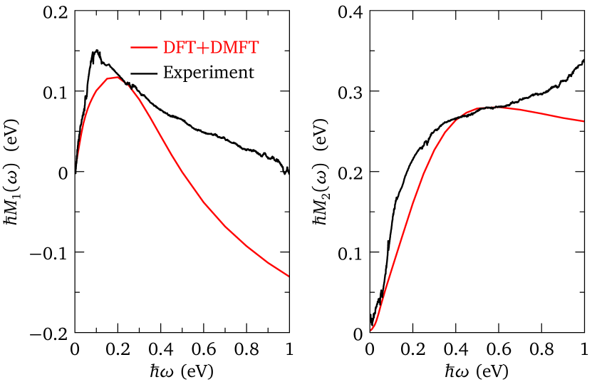
Figure SM15: Memory function; theory and experiment (both constructed using the experimentally determined $\hbar\omega_{p}=3.3$ eV).

also the LDA $t_{2g}$ bands that are renormalized by a factor of 4. Whereas at low energies these renormalized bands describe the data reasonably well, above $\sim 0.1$ eV (below $\sim-0.5$ eV) the dispersion abruptly increases, giving rise to the pronounced inverted waterfall structure.

Above those energies, broad and strongly dispersing resilient quasiparticle excitations appear very clearly in the $\bm{k}$-resolved spectral function. The excess conductivity found in the experiment and in our DFT+DMFT calculations is thus a consequence of highly dispersive states that exist above the Fermi energy. This is also reflected in the memory function, that is shown in Fig. SM15. The change of slope that appears due to the resilient quasiparticle states is seen clearly in the real part of the theoretical and experimental memory function.

References

- van Heumen et al. (2007) E. van Heumen, R. Lortz, A. B. Kuzmenko, F. Carbone, D. van der Marel, X. Zhao, G. Yu, Y. Cho, N. Barisic, M. Greven, C. C. Homes, and S. V. Dordevic, Phys. Rev. B 75, 054522 (2007).
- Katsufuji et al. (1996) T. Katsufuji, M. Kasai, and Y. Tokura, Phys. Rev. Lett. 76, 126 (1996).
- Hagen and Rubens (1903) E. Hagen and H. Rubens, Ann. Phys. (Leipzig) 4, 873 (1903).
- Berthod et al. (2013) C. Berthod, J. Mravlje, X. Deng, R. Žitko, D. van der Marel, and A. Georges, Phys. Rev. B 87, 115109 (2013).
- Blaha et al. (2001) P. Blaha, K. Schwarz, G. Madsen, D. Kvasnicka, and J. Luitz, WIEN2k, An augmented Plane Wave + Local Orbitals Program for Calculating Crystal Properties (Techn. Universitat Wien, Austria, ISBN 3-9501031-1-2., 2001).
- Georges et al. (1996) A. Georges, G. Kotliar, W. Krauth, and M. J. Rozenberg, Rev. Mod. Phys. 68, 13 (1996).
- Aichhorn et al. (2009) M. Aichhorn, L. Pourovskii, V. Vildosola, M. Ferrero, O. Parcollet, T. Miyake, A. Georges, and S. Biermann, Phys. Rev. B 80, 085101 (2009).
- Ambrosch-Draxl and Sofo (2006) C. Ambrosch-Draxl and J. O. Sofo, Computer Physics Communications 175, 1 (2006).
- Mravlje et al. (2011) J. Mravlje, M. Aichhorn, T. Miyake, K. Haule, G. Kotliar, and A. Georges, Phys. Rev. Lett. 106, 096401 (2011).
- Oguchi (1995) T. Oguchi, Phys. Rev. B 51, 1385 (1995).
- Singh (1995) D. J. Singh, Phys. Rev. B 52, 1358 (1995).
- Allen (2004) P. B. Allen, arXiv:cond-mat/0407777 (2004).
- Deng et al. (2013) X. Deng, J. Mravlje, R. Žitko, M. Ferrero, G. Kotliar, and A. Georges, Phys. Rev. Lett. 110, 086401 (2013).