Breathing dynamics based parameter sensitivity analysis of hetero-polymeric DNA

Abstract

We study the parameter sensitivity of hetero-polymeric DNA within the purview of DNA breathing dynamics. The degree of correlation between the mean bubble size and the model parameters are estimated for this purpose for three different DNA sequences. The analysis leads us to a better understanding of the sequence dependent nature of the breathing dynamics of hetero-polymeric DNA. Out of the fourteen model parameters for DNA stability in the statistical Poland-Scheraga approach, the hydrogen bond interaction $\epsilon_{hb}(\mathtt{AT})$ for an $\mathtt{AT}$ base pair and the ring factor $\xi$ turn out to be the most sensitive parameters. In addition, the stacking interaction $\epsilon_{st}(\mathtt{TA}-\mathtt{TA})$ for an $\mathtt{TA}-\mathtt{TA}$ nearest neighbor pair of base-pairs is found to be the most sensitive one among all stacking interactions. Moreover, we also establish that the nature of stacking interaction has a deciding effect on the DNA breathing dynamics, not the number of times a particular stacking interaction appears in a sequence. We show that the sensitivity analysis can be used as an effective measure to guide a stochastic optimization technique to find the kinetic rate constants related to the dynamics as opposed to the case where the rate constants are measured using the conventional unbiased way of optimization.

I Introduction

Hydrogen bonding between the complementary base pairs ($\mathtt{AT}$ and $\mathtt{GC}$) is the origin for the Watson Crick double helical DNA structure watson . The secondary interaction via the nearest neighboring stacking interaction also has a major contribution towards the DNA structure. The base pair stacking compensates the repulsive electrostatic force of phosphate groups of the two complementary bases which come closer due to hydrogen bonding, henceforth giving stability to the helical conformation. Although this double helix is the most stable form of DNA, it is not a static one frank ; wartell ; grosberg ; poland1 ; poland . The hydrogen bonds can intermittently open up and rejoin, even at room temperature and normal salt concentration, without damaging the core of the nucleotide. This transient denatured zone in a DNA polymer is commonly known as a bubble. As the total energy needed to open up a base pair depends on the nature of that base pair (hydrogen bond interaction) as well as its neighborhood (stacking interaction), the probability of bubble formation becomes a function of the DNA sequence, i.e it is connected to the stability profile of a genome. It is also important to mention that in most natural DNA, the opening probability is much higher due to torsional stress bauer ; jeon . The breathing dynamics of bubble plays a crucial role in the functioning of DNA pollock ; pant ; ambj1 ; sokolov ; yeramian ; choi ; nowak ; zoli ; phelps . Fundamental biological processes like replication and transcription largely rely on the local denaturation. A recent study on the interaction between the nucleoid-associated protein Fis and DNA in E. coli suggests that Fis-DNA interaction is controlled by DNA breathing dynamics and can be regulated experimentally via different nucleotide modifications nowak . The physical properties of the DNA direct the biological functioning of the living system. DNA breathing is thus a good problem to study, both with respect to its physical and biological perspective.

Many experimental techniques, such as, circular dichroism cantor , UV spectroscopy cantor , calorimetry senior , fluorescence resonant energy transfer (FRET) measurements gelfand can map out the melting profile of DNA. Using single molecule florescence correlation spectroscopy, breathing dynamics has been monitored and multistep relaxation kinetics with characteristic time scale has been accounted from the study altan ; kathy . Experimental studies have also been performed to explore correlations between the dynamics of hetero-polymeric DNA with the biological activities of nucleic acid enzymes phelps . Theoretical models of the dynamics have also been established based on the DNA free energy landscape hanke ; bicout ; bar ; novotny ; fogedby . Another way of studying breathing dynamics is by carrying out a stochastic simulation ambj2 ; ambj3 using the Gillespie Algorithm gill1 ; gill2 .

Sequence sensitivity is one of the pivotal motivations for studying DNA breathing dynamics. From the time series data of the dynamics, information about DNA sequence and its stability parameters can be estimated. Single DNA manipulation techniques can produce stability parameters and can account for the strong dependence on salt concentration of the breathing dynamics huguet . In one of our previous communications we showed that the conjunction of breathing dynamics of hetero-polymeric DNA with one of the stochastic optimization technique, namely Simulated Annealing, can provide data regarding the stability parameters, as well as the activation energy and critical exponent with good accuracy talukder1 . However, the dependence of the breathing dynamics on the individual parameters had not been discussed in earlier work. We here ask whether can we quantify the relative influence of the system parameters on the breathing dynamics? To answer this question we quantify the sensitivity of the stability parameters as well as the activation energy and the critical exponent with respect to the breathing dynamics of a hetero-polymeric DNA using the approach of sensitivity analysis (SENSA).

SENSA is used to understand the relative importance of input parameters with respect to the system output. Generally SENSA is of two types, local and global saltelli ; marino . Local SENSA is based on gradient calculation and can account for the local effect of that particular input parameter on the output, for which the calculation is performed. It generally fails to provide accurate results when all the input parameters come into consideration simultaneously. The global SENSA follows a statistical formulation. The fundamental theory regarding the global strategy is how the variance of the output is guided by the perturbation on individual input parameters. Global SENSA is thus a sampling based technique. There are various ways to calculate the global SENSA and the success of these techniques are system specific. One of the two most popular method is the measure of correlations between the input and output parameters which is essentially used for systems whose output varies monotonically with the input. But for those systems which do not follow a monotonic trend, the decomposition of the variance represents the best choice for determining sensitivity index. The most reliable variance based method is eFAST proposed by Saltelli et. al. saltelli1 . eFast is actually based on the Fourier Amplitude Sensitivity Test (FAST), developed by Cukier et.al cukier ; cukier1 and Schaibly et.al schaibly . In the variance based sensitivity test the partitioning of variance (of output) is done for determining what fraction of the variance in the output occurs due to the variation of each input parameters. This is known as the partial variance of output. The sensitivity of a particular input parameter is estimated using the ratio of the partial variance of the output (for that particular input) to the total output variance.

SENSA has a wide range of application in different fields like economics pannell , environmental science hornberger , systems biology zi1 , or chemical kinetics saltelli . Biologists use SENSA to understand the robustness of the model output with respect to the variation in model inputs. This study also helps to analyze the dynamical behavior of the biological model. In chemistry, there is also a long history of applying SENSA in chemical kinetics. The SENSA of rate constants on the reaction kinetics is an important way to understand a kinetic scheme tohsato ; talukder2 . It also has profound implications on parameter optimization talukder2 .

We use the correlation coefficient as a measure of the the index of sensitivity for the parameters associated with the breathing dynamics as the breathing dynamics is monotonically related to these parameters. In this communication the Pearson correlation coefficient (CC), the rank correlation coefficient (RCC), and the partial rank correlation coefficient (PRCC) book ; hora are calculated for three different DNA sequences and their performance compared. We also discuss the relevance of the SENSA on the parameter optimization and how these results can dramatically influence an optimization process. Specifically, we study how the DNA breathing parameters, as described by the Poland-Scheraga model, respond when subjected to a SENSA test. In other words, the gradation of these model parameters on the basis of sensitivity will give us a picture as to which of the model parameters play a more important role in controlling the breathing dynamics. We also pursue the important question whether the sensitivity order is dependent on the nature of the sequence. In an earlier work, stochastic optimization (Simulated Annealing) was demonstrated to extract reliably the interaction energies in DNA breathing talukder1 . In the present work we show that taking the sensitivity of individual parameters into consideration, an optimization procedure becomes more efficient in the determination of interaction energies of DNA breathing data. The Genetic Algorithm, which has a completely different philosophy of operation as that of Simulated Annealing, is used as the stochastic optimizer in this work. One of the reason of using Genetic Algorithm over Simulated Annealing is that the Genetic Algorithm, because of the relatively large search space it can sample and exploit, requires a smaller number of optimization steps to converge than that of Simulated Annealing talukder2 .

II Breathing Dynamics in DNA

The stability of the double helical DNA hetero-polymer can be explained by considering the two types of Watson-Crick hydrogen bond interaction between the complementary bases $\mathtt{A}$ and $\mathtt{T}$, and $\mathtt{G}$ and $\mathtt{C}$ as well as the ten types of stacking interactions between the nearest neighbor base pairs. In numbers, the net free energy released due to opening of a base pair, whose nearest neighbor base pair to one side is already denatured, is quite low, due to the fact that enthalpy cost and entropy gain almost cancel. Thus the free energy involved to break the strongest interaction, a $\mathtt{GC}$ base pair stacked with a $\mathtt{CG}$ downstream of the DNA sequence, is around $\sim 3.9$ $k_{B}T$ (at 37⁰), whereas the denaturation of an $\mathtt{AT}$ base pair with a downstream $\mathtt{TA}$ is marginally unstable with free energy change $\sim 0.1$ $k_{B}T$ (at 37⁰) krueger . The unzipping of DNA double helix is an entropy driven process as it is basically a transformation from an ordered to disordered conformation. The high binding enthalpy is compensated by the entropy gain. But for a bubble initiation the activation energy is very high, of the order of 7-12 $k_{B}T$ (for weakest and strongest respectively) as breaking of two stacking interactions along with the disruption of a hydrogen bond are concerned. Thus it is justified to assume that bubble events are rare and two bubbles are well separated below the melting temperature.

A bubble formation event may be denoted by the position of the left zipper fork ($x_{L}$) and the size of the bubble ($m$) in terms of the right zipper fork $x_{R}=x_{L}+m+1$. One can visualize the breathing dynamics as a random walk of a bubble on a triangular lattice of $x_{L}$ and $m$ with forbidden horizontal transition. The Master equation depicting this process

$$\frac{\partial P(x_{L},m,t)}{\partial t}=\mathbb{W}P(x_{L},m,t),$$ (1)

where $P(x_{L},m,t)$ is the probability of the occurrence of a bubble of size $m$ at the left zipper fork $x_{L}$ at a time $t$ and $\mathbb{W}$ matrix include all the allowed transition rates from the state $(x_{L},m)$ in the triangular lattice. The transfer rates are defined in terms of the Boltzmann factor of hydrogen bonding interaction and stacking interaction

$$u_{hb}(x)=\exp\left(\frac{\epsilon_{\mathrm{hb}}(x)}{k_{B}T}\right),u_{st}(x)=\exp\left(\frac{\epsilon_{\mathrm{st}}(x)}{k_{B}T}\right).$$ (2)

In Eq. (2), $u_{hb}(x)$ is the Boltzmann factor for hydrogen bond at base pair position $x$ and $u_{st}(x)$ is the Boltzmann factor for nearest neighbor stacking interaction between the base pairs at $x-1$ and $x$, respectively. At $t\rightarrow\infty$, $P(x_{L},m,t)$ from Eq. (1) equilibrates to a probability distribution obtained from the statistical mechanical Poland-Scheraga model poland1 ; poland of the DNA double helix. The equilibrium probability of a bubble of size $m$ and left zipper fork position $x_{L}$ can be written as

$$P_{\mathrm{eq}}(x_{L},m)=\frac{\mathbb{Z}(x_{L},m)}{\mathbb{Z}(0)+\sum_{m=1}^{M}\sum_{x_{L}=0}^{M-m}\mathbb{Z}(x_{L},m)},$$ (3)

where $\mathbb{Z}(x_{L},m)$ is the bubble partition function

$$\mathbb{Z}(x_{L},m)=\frac{\xi^{\prime}}{(1+m)^{c}}\prod_{x=x_{L}+1}^{x_{L}+m}u_{\mathrm{hb}}(x)\prod_{x=x_{L}+1}^{x_{L}+m+1}u_{\mathrm{st}}(x).$$ (4)

Eq. (4) is for bubble size $m>0$. If $m=0$, $\mathbb{Z}(0)=1$. Moreover, $\xi^{\prime}=2^{c}\xi$, where $\xi$ is the ring factor which contributes to the cooperativity factor. The cooperativity factor is the free energy cost for bubble activation. The ring factor is the key element for the formation of a small constrained loop in DNA double helix krueger . Finally, $c$ is the critical exponent and is related to the entropy factor during bubble formation kaiser2014 . The term $(1+m)^{-c}$ accounts for the loss of entropy during the formation of a polymer loop. From the probability expression one may write the equilibrium mean bubble size $\langle m\rangle$, for a sequence of base pair of length $M$ as

$$\langle m\rangle=\frac{\sum_{m=1}^{M}m\sum_{x_{L}=0}^{M-m}\mathbb{Z}(x_{L},m)}{\mathbb{Z}(0)+\sum_{m=1}^{M}\sum_{x_{L}=0}^{M-m}\mathbb{Z}(x_{L},m)}.$$ (5)

III Sensitivity Analysis of the DNA Stability Parameters

Sensitivity analysis is an efficient tool to understand the degree of susceptibility of the system with respect to different input parameters. The biological functions of DNA are actually affected by the bubble dynamics as intermittent bubble opening of base pair helps in binding of RNA polymerase, or single-stranded DNA binding proteins, etc. Thus it is relevant to study the effect of the stability parameters on the breathing dynamics. To this end we use SENSA as a tool to measure the different weights of the DNA breathing model parameters (hydrogen bond interaction $\epsilon_{hb}$ and stacking interaction $\epsilon_{st}$) on the process. As mentioned in the previous section, the equilibrium probability distribution for bubble formation also involves the ring factor factor $\xi$ and the critical exponent factor $c$, which should have significant effect on bubble formation. This leads us to consider all fourteen model parameters in the SENSA, namely, two hydrogen bond interactions, ten nearest neighbor stacking interactions, as well as the ring factor and critical exponent.

In order to quantify the effect of all fourteen parameters on the breathing dynamics of hetero-polymeric DNA, we consider the mean bubble size $\langle m\rangle$ as the measure for the breathing dynamics, which can be quantitatively determined via experiment. The breathing dynamics of hetero-polymeric DNA is sensitive to the DNA sequence ambj2 , which leads us to consider three different DNA sequences, the promoter sequence of the T7 phage ambj2 , as well as the L42B12 zeng and AdMLP choi sequences, for the present study to get a complete picture of sensitivity of the breathing parameters. The promoter sequence of T7 phage is used as the first sequence and is represented as

5’-aTGACCAGTTGAAGGACTGGAAGTAATACGACTC

$$\texttt{AGTATAGGGACAATGCTTAAGGTCGCTCTCTAGGAg -3'}.$$

Firstly, to start the SENSA test, we generate scatter plots of the mean bubble size vs all the parameters for the promoter sequence of T7 phage, which gives a first hand qualitative picture of sensitivity. To generate a scatter plot for a particular input parameter against an output, all the input parameters of the system under consideration are perturbed simultaneously and the output is calculated using the set of perturbed parameters. If the output thus generated using the perturbed set of parameters is plotted (typically known as input vs output scatter plot) against the values of one specific parameter and falls in a narrow region around a virtual straight line, the corresponding input parameter seems to be more important with respect to that output parameter and is considered to have higher degree of sensitivity. Points dispersed in a circular region in the scatter plot denotes less or no correlation between the input and the output. Fig.1 represents the set of the scatter plots generated using the above mentioned procedure for the promoter sequence of T7 phage. The input data has been picked up by a random process with the mean situated at the reported value (of that model parameter) krueger ; richard and the width of the perturbation being $\pm$5$\%$ of the reported value. For most of the input parameters, plots appear as a dispersed set of points. Only in the scatter plots for the ring factor ($\xi$) and $\epsilon_{hb}(\mathtt{AT})$, the distribution of points falls in a narrow strip (or follow a definite direction) and hence could be considered to be more sensitive parameters related to DNA breathing dynamics.

Figure 1: Scatter plots of the mean bubble size versus the parameters associated with the breathing dynamics of hetero-polymeric DNA, for the promoter sequence of the T7 phage.

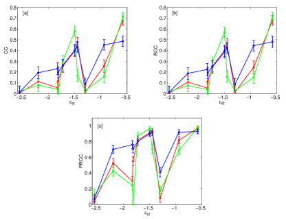
Figure 2: (Color online) Correlation coefficients: (a) CC, (b) RCC, and (c) PRCC versus the free energy of stacking interactions. The red, green, and blue lines are for the promoter sequence of the T7 phage, the L42B12, and the AdMLP sequences, respectively. The stacking interactions show similar trends for all the three DNA sequences.

As the expression for calculating $\langle m\rangle$ (see Eq. (5)) is monotonic with respect to all the fourteen model parameters, we use the measured correlation coefficient using different techniques as the measure of sensitivity index of these model parameters. To this end, we estimate the Pearson correlation coefficient (CC), the Spearman or rank correlation coefficient (RCC), and the partial rank correlation coefficient (PRCC) (for detail, see Appendix A) for the T7 phage DNA. The results are shown in Table 1. The set of input parameters is chosen in a similar manner as used for generating the scatter plots, while calculating correlation coefficients (see Appendix A for discussion of the implementation). Specifically, the correlation coefficients are computed from a set of 100,000 data points for the generation of input and output data. The first set of CC, RCC and PRCC in Table 1, designated as “All parameters”, are calculated by varying all the fourteen model parameters simultaneously. The values of coefficients obtained from the raw data (CC) and rank transformed data (RCC) are very close, as the mean bubble size shows a linear dependence on the input parameters. However, the PRCC is much higher in magnitude than the CC and the RCC, which signifies that the effect of a particular input on the output is not independent of the other input parameters. Hence, PRCC gives a clearer picture of the parameter sensitivity. The set of correlation coefficients for all the stability factors (only $\epsilon_{hb}$ and $\epsilon_{st}$) and for the stacking interactions (only $\epsilon_{st}$) are also calculated and are presented in Table 1 under the column heading of “Excluding $c$ $\&$ $\xi$” and “Excluding $c$, $\xi$ $\&$ $\epsilon_{hb}$”, respectively. These are calculated by perturbing all the parameters except the excluded parameters which are kept fixed at the corresponding literature values. This is done to check how the parameter sensitivity order changes with the gradual decrease in the set of parameter variation. Results show that an increase in the values of different correlation coefficients occurs (as calculated by adopting CC, RCC and PRCC), but the relative order of the sensitivity remains the same, which is a signature of the linear dependence of the input parameters.

Table 1: CC, RCC, and PRCC values for the promoter sequence of the T7 phage (the importance of the numbers in bold are discussed in Sec III)

Parameter		All parameters			Excluding			Excluding
					$c$ & $\xi$			$c$, $\xi$ & $\epsilon_{hb}$
	CC	RCC	PRCC	CC	RCC	PRCC	CC	RCC	PRCC
$\epsilon_{st}$ ($\mathtt{AT-AT}$)	0.135	0.128	0.589	0.168	0.160	0.711	0.249	0.239	0.818
$\epsilon_{st}$ ($\mathtt{TA-TA}$)	0.358	0.346	0.890	0.436	0.420	0.938	0.676	0.679	0.969
$\epsilon_{st}$ ($\mathtt{AA-TT}$)	0.207	0.199	0.752	0.257	0.245	0.843	0.395	0.382	0.913
$\epsilon_{st}$($\mathtt{GA-TC}$)	0.063	0.062	0.328	0.075	0.071	0.422	0.124	0.118	0.550
$\epsilon_{st}$($\mathtt{CA-TG}$)	0.134	0.129	0.594	0.168	0.160	0.709	0.256	0.246	0.819
$\epsilon_{st}$($\mathtt{AG-CT}$)	0.251	0.242	0.807	0.310	0.297	0.882	0.471	0.459	0.937
$\epsilon_{st}$($\mathtt{AC-GT}$)	0.054	0.051	0.301	0.073	0.070	0.403	0.112	0.108	0.529
$\epsilon_{st}$($\mathtt{GG-CC}$)	0.030	0.030	0.158	0.035	0.032	0.209	0.052	0.050	0.295
$\epsilon_{st}$($\mathtt{CG-CG}$)	0.012	0.011	0.038	0.010	0.010	0.063	0.014	0.013	0.084
$\epsilon_{st}(\mathtt{GC-GC})$	0.002	0.002	0.022	0.000	0.001	0.031	0.009	0.008	0.034
$\epsilon_{hb}(\mathtt{AT})$	0.624	0.622	0.961	0.760	0.768	0.980
$\epsilon_{hb}(\mathtt{GC})$	0.079	0.076	0.390	0.096	0.091	0.502
$\xi$	0.556	0.550	0.951
c	-0.101	-0.096	-0.467

It is further evident from Fig. 1 and Table 1 that the hydrogen bond interaction energy for an $\mathtt{AT}$ base pair $\epsilon_{hb}(\mathtt{AT})$ and the ring factor $\xi$ are highly sensitive among the set of model parameters controlling the breathing dynamics. However, it is also interesting to analyze the sensitivity of different stacking interactions on the breathing dynamics. The parameter $\epsilon_{st}(\mathtt{TA-TA})$ shows the highest degree of correlation among all the stacking energies, which is actually the weakest interaction in DNA double helix. Frequent bubble events in the weaker $\mathtt{TATA}$ motif, a key element in this T7 promoter sequence, also justify the SENSA due to the effected greater probability of bubble formation. The order of sensitivity of the parameters for stacking interaction, as found out by the calculation of correlation coefficients, for the sequence T7 phage promoter is thus as follows

$$\epsilon_{st}(\mathtt{TA-TA})>\epsilon_{st}(\mathtt{AG-CT})>\epsilon_{st}(\mathtt{AA-TT})>\epsilon_{st}(\mathtt{AT-AT})$$

$$\approx\epsilon_{st}(\mathtt{CA-TG})>\epsilon_{st}(\mathtt{GA-TC})>\epsilon_{st}(\mathtt{AC-GT})>\epsilon_{st}(\mathtt{GG-CC})$$

$$>\epsilon_{st}(\mathtt{CG-CG})>\epsilon_{st}(\mathtt{GC-GC}).$$ (7)

Eq. (III) shows that sensitivity of the stacking interaction energies involved with AT base pair are higher compared to the stacking interaction energies between the two neighboring GC bases. One of the reasons may be the presence of fewer numbers of $\epsilon_{st}(\mathtt{CG-CG})$ and $\epsilon_{st}(\mathtt{GC-GC})$ in the promoter sequence of T7 phage (both appear only twice). However, another stacking interaction between two neighboring $\mathtt{GC}$ ($\epsilon_{st}(\mathtt{GG-CC})$) appears relatively frequently in the sequence. Thus one cannot generalize the effectivity of a particular stacking interaction energy on the breathing dynamics from the point of view of the number of appearance of that particular stacking interaction, and thus we are led to conclude that both the number of occurrences and the nature of the stacking interaction affect the sensitivity order. To check how the relative sensitivity order of these model breathing parameters, mainly the stacking interactions, gets altered due to the sequence of hetero-polymeric DNA, we performed the above mentioned calculation for the correlation coefficients (CC, RCC, PRCC) on two other different DNA sequences. These two other DNA hetero-polymeric chains are L42B18 and AdMLP with the following sequences

$$\texttt{5'-cCGCCAGCGGCGTTAATACTTAAGTATTATGGCCGCTGCGCc -'3},$$ (8)

and

5’-gCCACGTGACCAGGGGTCCCCGCCGGGGGGGTATAAAAGGGGCGGACC

$$\texttt{TCTGTTCGTCCTCACTGTCTTCCGGATCGCTGTCCAg -'3}.$$ (9)

The list of correlators: CC, RCC, and PRCC obtained by varying all the model parameters, for the two sequences (8) and (III) are listed in Tab. 2 and Tab. 3. The correlation coefficients related to $\xi$ and $c$ should be independent of the sequence as indeed observed. In the case of the hydrogen bond energies, $\epsilon_{hb}(\mathtt{AT})$ has a much higher correlation coefficient compared to $\epsilon_{hb}(\mathtt{GC})$ for all three sequences. However, in AdMLP the value of CC (also RCC and PRCC) for $\epsilon_{hb}(\mathtt{GC})$ is higher than the other two sequences, as in AdMLP the $\mathtt{GC}:\mathtt{AT}$ number ratio is much higher than in the other two sequences. The stacking interactions in hierarchical order of sensitivity for the L42B12 and AdMLP DNA sequences are

$$\epsilon_{st}(\mathtt{TA-TA})>\epsilon_{st}(\mathtt{AA-TT})>\epsilon_{st}(\mathtt{AT-AT})>\epsilon_{st}(\mathtt{AG-CT})$$

$$>\epsilon_{st}(\mathtt{CA-TG})>\epsilon_{st}(\mathtt{AC-GT})>\epsilon_{st}(\mathtt{GG-CC})$$

$$>\epsilon_{st}(\mathtt{CG-CG})>\epsilon_{st}(\mathtt{GC-GC})>\epsilon_{st}(\mathtt{GA-TC}),$$

and

$$\epsilon_{st}(\mathtt{TA-TA})>\epsilon_{st}(\mathtt{CA-TG})\sim\epsilon_{st}(\mathtt{AG-CT})>\epsilon_{st}(\mathtt{AA-TT})$$

$$>\epsilon_{st}(\mathtt{AT-AT})>\epsilon_{st}(\mathtt{GG-CC})>\epsilon_{st}(\mathtt{GA-TC})$$

$$>\epsilon_{st}(\mathtt{AC-GT})>\epsilon_{st}(\mathtt{CG-CG})>\epsilon_{st}(\mathtt{GC-GC}).$$

By comparing the relative sensitivity order of the three analyzed sequences, the sensitivity of stacking interaction between two neighboring GC bases ($\epsilon_{st}(\mathtt{GG-CC})$, $\epsilon_{st}(\mathtt{CG-CG})$, and $\epsilon_{st}(\mathtt{GC-GC})$) are found to be very low for T7 and L42B18, but in AdMLP the correlation coefficient value (see in Table 3) of $\epsilon_{st}(\mathtt{GG-CC})$ is relatively high. This happens as the AdMLP sequence has higher $\mathtt{GC}$ content and the $\epsilon_{st}(\mathtt{GG-CC})$ stacking interaction appears 24 times in this sequence. But $\epsilon_{st}(\mathtt{TA-TA})$ still shows the highest correlation value among all stacking interaction energies for all three sequences though it appears only twice in the AdMLP sequence. This is a signature of the fact that the $\mathtt{TA-TA}$ stacking interaction has an overriding influence on the breathing process even in a situation where its numbers are low. A table containing the number of appearance of each stacking interaction in all the three sequences is given for reference (see Table  4). Our objective to perform the SENSA for the sequences L42B12 and AdMLP along with the T7 phage promoter sequence is to figure out how the sensitivity order of the stacking interaction parameters changes with the variation of DNA sequences. For this purpose a pictorial presentation of the free energy of stacking interactions versus their correlation coefficients (CC, RCC and PRCC) are given for all three DNA sequences in Fig.2: we see that the general trend of the sensitivity order remains more or less unchanged in these three different DNA sequences. One may thus group out the stacking interactions such that $\epsilon_{st}(\mathtt{AT-AT})$, $\epsilon_{st}(\mathtt{TA-TA})$, $\epsilon_{st}(\mathtt{AA-TT})$, $\epsilon_{st}(\mathtt{CA-TG})$, and $\epsilon_{st}(\mathtt{AG-CT})$ are more sensitive towards bubble opening than the other five stacking interactions. This results together lead us to conclude that the nature of the stacking interaction is predominant over the number of appearance of that particular stacking interaction in calculating the sensitivity for a hetero-polymeric DNA sequence.

IV Discussion and Conclusion

Sensitivity analysis can help in a rigorous study of a system. We quantified the sensitivity of bubble formation with respect to the stability parameters (as given by the Poland-Scheraga model), which leads us to a better understanding of the sequence dependent nature of the breathing dynamics of hetero-polymeric DNA. The general trend of this parameter SENSA as evaluated from our calculations is that it does not significantly depend on the nature of the DNA sequence. We showed that the number of occurrences of a particular interaction (hydrogen bond interaction or stacking interaction) is not the major factor in the degree of sensitivity. Rather, the specific nature of a particular interaction is the major player, even in a situation where its number of occurrences in a DNA sequence is smaller. Generally, the SENSA also shows that the bubble opening free energy $\xi$ and the hydrogen bonding free energy $\epsilon_{hb}(\mathtt{AT})$ are always highly sensitive parameters. These results will help in a better understanding of the relative probability of bubble opening and how it varies with the change in DNA sequences.

The sensitivity data, as revealed and discussed in the previous section, has its own role in grading the different interaction types in order of importance, but the information can be used for other important studies as well, like an optimization problem to find out the correct values of the breathing dynamics parameters. The SENSA data if used properly can have a significant influence during parameter optimization of the system. All parameters may not equally affect or influence the output. If one exploits the parameters having higher sensitivity more than the other parameters during optimization, the convergence may occur faster than a simulation in which all parameters are searched with equal weights.

Table 2: CC, RCC, and PRCC values of the L42B18 sequence (the importance of the numbers in bold are discussed in Sec III)

Parameter		All parameters			Excluding			Excluding
					$c$ & $\xi$			$c$, $\xi$ & $\epsilon_{hb}$
	CC	RCC	PRCC	CC	RCC	PRCC	CC	RCC	PRCC
$\epsilon_{st}(\mathtt{AT-AT})$	0.170	0.163	0.681	0.202	0.192	0.772	0.300	0.287	0.876
$\epsilon_{st}(\mathtt{TA-TA})$	0.404	0.393	0.912	0.476	0.461	0.946	0.715	0.716	0.976
$\epsilon_{st}(\mathtt{AA-TT})$	0.333	0.323	0.873	0.389	0.374	0.920	0.578	0.566	0.963
$\epsilon_{st}(\mathtt{GA-TC})$	0.006	0.006	0.003	0.005	0.006	0.004	0.002	0.002	0.000
$\epsilon_{st}(\mathtt{CA-TG})$	0.093	0.087	0.441	0.105	0.100	0.536	0.158	0.151	0.689
$\epsilon_{st}(\mathtt{AG-CT})$	0.096	0.091	0.456	0.114	0.108	0.555	0.167	0.158	0.705
$\epsilon_{st}(\mathtt{AC-GT})$	0.040	0.039	0.237	0.052	0.050	0.303	0.074	0.069	0.421
$\epsilon_{st}(\mathtt{GG-CC})$	0.023	0.021	0.122	0.027	0.025	0.160	0.033	0.032	0.243
$\epsilon_{st}(\mathtt{CG-CG})$	0.016	0.015	0.089	0.018	0.017	0.114	0.024	0.023	0.171
$\epsilon_{st}(\mathtt{GC-GC})$	0.008	0.008	0.065	0.012	0.011	0.085	0.025	0.024	0.126
$\epsilon_{hb}(\mathtt{AT})$	0.633	0.633	0.963	0.742	0.748	0.978
$\epsilon_{hb}(\mathtt{GC})$	0.039	0.037	0.241	0.056	0.053	0.303
$\xi$	0.508	0.500	0.943
c	-0.108	-0.104	-0.514

Table 3: CC, RCC, and PRCC values of the AdMLP sequence (the importance of the numbers in bold are discussed in Sec III)

Parameter		All parameters			Excluding			Excluding
					$c$ & $\xi$			$c$, $\xi$ & $\epsilon_{hb}$
	CC	RCC	PRCC	CC	RCC	PRCC	CC	RCC	PRCC
$\epsilon_{st}(\mathtt{AT-AT})$	0.128	0.123	0.575	0.160	0.152	0.699	0.265	0.258	0.797
$\epsilon_{st}(\mathtt{TA-TA)}$	0.242	0.233	0.792	0.306	0.294	0.877	0.482	0.476	0.927
$\epsilon_{st}(\mathtt{AA-TT})$	0.196	0.187	0.730	0.253	0.241	0.833	0.405	0.397	0.898
$\epsilon_{st}(\mathtt{GA-TC})$	0.096	0.092	0.466	0.122	0.115	0.589	0.198	0.191	0.702
$\epsilon_{st}(\mathtt{CA-TG})$	0.219	0.210	0.768	0.281	0.270	0.861	0.453	0.446	0.918
$\epsilon_{st}(\mathtt{AG-CT})$	0.216	0.208	0.756	0.273	0.261	0.850	0.437	0.430	0.911
$\epsilon_{st}(\mathtt{AC-GT})$	0.096	0.091	0.455	0.122	0.116	0.584	0.195	0.188	0.695
$\epsilon_{st}(\mathtt{GG-CC})$	0.113	0.108	0.523	0.146	0.139	0.651	0.235	0.228	0.759
$\epsilon_{st}(\mathtt{CG-CG})$	0.042	0.040	0.225	0.051	0.048	0.313	0.083	0.080	0.404
$\epsilon_{st}(\mathtt{GC-GC})$	0.027	0.023	0.034	0.065	0.056	0.047	0.015	0.015	0.069
$\epsilon_{hb}(\mathtt{AT})$	0.587	0.583	0.956	0.748	0.756	0.978
$\epsilon_{hb}(\mathtt{GC})$	0.176	0.169	0.674	0.211	0.201	0.787
$\xi$	0.612	0.609	0.960
c	-0.098	-0.093	-0.465

We optimized all parameters associated with the breathing dynamics taking the equilibrium distribution function generated by mimicking the experimental scenario altan , as the objective during optimization (see Appendix B). We used the Genetic Algorithm (GA) gold as the optimizer and the promoter sequence of T7 Phage for this study. Fig.3 represents the cost profile versus the number of GA steps for different runs with different extent of constraints in searching the sensitive parameters. The cost function (see Appendix B) is a measure of how close we are to obtaining our solution. When the cost tends to zero the actual solution is found out. The solid line is the profile for the normal optimization, during which no additional condition is imposed on the optimizer. But the other lines represent cost profiles, for which the optimization was biased to sample the sensitive parameters more by allowing it to mutate or get sampled more than the others. In GA, mutation occurs with a probability (mutation probability) which is set initially. Generally there is no bias in the choice of variables for mutation. We incorporated a condition in the choice of variable selected to undergo mutation. The more sensitive parameters have a higher probability to be selected for mutation. In Fig.3 the dashed line represents the profile where, the cumulative probability for $\xi$ and $\epsilon_{hb}(\mathtt{AT})$ (the most sensitive parameters) to be chosen for mutation is 20$\%$ and the rest is the cumulative probability for the other parameters. The cost profile with 60$\%$ of such a cumulative probability for the sensitive parameters is denoted by the dotted line. The dashed line (20$\%$) falls at a greater rate than the solid one, but the gain in the initial convergence is much more prominent for the dotted line (60$\%$). In spite of this gain, the plateau region in the optimization profile starts at a higher cost in the case of the dotted line than for the solid line. The probable reason may be the incomplete search of the other relatively less sensitive parameters. Thus we designed the optimization scheme such that initially the search would be highly biased towards the sensitive parameters and after certain steps of optimization, the cumulative probability to be picked up for mutation, of those higher sensitive parameters would be decreased. The close-dotted line in Fig.3 was generated by keeping this cumulative probability 60$\%$ initially (upto 200 GA steps) and then it is decreased to 20$\%$. This strategy of gradual reduction in sampling importance (kept high initially and decreased later) of the more sensitive parameters is the ideal strategy to handle the present problem in a more computationally cost-efficient way.

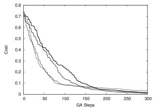
Figure 3: Cost profile obtained for different cases of optimization. The solid line represents unconstrained optimization, the dashed and dotted lines are obtained by keeping the cumulative probability for mutation of the sensitive parameters at 20$\%$ and 60$\%$, respectively. The close-dotted line is generated by keeping this cumulative probability at 60 $\%$ up to 200 GA steps, and then at 20$\%$ for the rest of the optimization.

Table 4: List of the number of occurrance of different stacking interactions in the three studied DNA sequences (the importance of the numbers in bold are discussed in Sec III)

Stacking interaction	$\epsilon_{st}$	T7		L42B18		AdMLP
$(\mathtt{AT-AT})$	1.729409	4		3		2
$(\mathtt{TA-TA})$	0.579800	6		5		2
$(\mathtt{AA-TT})$	1.499484	7		5		5
$(\mathtt{GA-TC})$	1.819371	11		0		12
$(\mathtt{CA-TG})$	0.939677	7		3		8
$(\mathtt{AG-CT})$	1.455363	14		4		9
$(\mathtt{AC-GT})$	2.199241	9		3		11
$(\mathtt{GG-CC})$	1.829370	7		6		24
$(\mathtt{CG-CG})$	1.299554	2		5		7
$(\mathtt{GC-GC})$	2.559130	2		7		4

Appendix A Correlation Coefficient

A simple way to examine a given parameter’s sensitivity is to obtain the degree of correlation of various input parameters to the output. The Correlation Coefficient is a quantity to measure how strong the output of a system is linearly associated with the particular input parameter. It also accounts for the direction (positive or negative) of this linear association. Thus it may be used as sensitivity index for a system in which the output varies linearly with the input variables, as it actually accounts for the perturbation on the output when input parameters are varied. The Correlation Coefficient of a particular parameter is fundamentally the measure of covariance between the output and that of input parameter, which is then normalised by dividing with the product of the standard deviation of input and output,

$$r_{x_{j}y}=\frac{\sum_{i=1}^{N}(x_{ij}-\bar{x}_{j})(y_{i}-\bar{y})}{\sqrt{\sum_{i=1}^{N}(x_{ij}-\bar{x}_{j})^{2}\sum_{i=1}^{N}(y_{i}-\bar{y})^{2}}}.$$ (12)

Here $r_{x_{j}y}$ is the correlation coefficient of the input parameter $x_{j}$ and output $y$, $\bar{x}_{j}$ and $\bar{y}$ are the mean of input and output, respectively and $N$ is the number of sampling. The value of $r_{x_{j}y}$ varies from -1 to +1. The ‘+’ or ‘-’ sign denotes the direction of the linear dependence, i.e, whether the output data increases or decreases with the increase in input parameter. For higher magnitudes of $r_{x_{j}y}$ the effect of that particular input parameter will be larger on the output parameter. Then that particular input parameter is said to be highly sensitive with respect to that output. A very low value of the correlation coefficient means that the output will differ only a little even when the perturbation on input is very high which signifies the lesser sensitivity of that input. If $r_{x_{j}y}$ is calculated from the raw data of input and output using Eq. (12), it is known as Pearson correlation coefficient (CC).

The parameter dependence may not always be linear. The Pearson correlation coefficient is inadequate to show the actual picture of sensitivity of the system in that case. If one uses rank transformed data instead of the raw data of both the input and output parameters to calculate the correlation coefficient (known as rank correlation coefficient (RCC)), it will account for the nonlinear, yet monotonic trend of parameter dependence. The formal name of RCC is Spearman Correlation Coefficient.

The Partial Rank correlation coefficient (PRCC) accounts for the dependence of a particular input with the output after deducting the effect of other inputs. PRCC of a set of inputs $x_{j}$ and output $y$ may be calculated as the RCC of $x_{j}-\tilde{x}_{j}$ and $y-\tilde{y}$, where $\tilde{x}_{j}$ and $\tilde{y}$ account for the effect of other input parameters on that particular input $x_{j}$ and output $y$. These can be measured following the regression model marino

$$\tilde{x}_{j}=c_{0}+\sum_{l\neq{j}}^{k}c_{l}x_{l},\;\tilde{y}=b_{0}+\sum_{l\neq{j}}^{k}b_{l}x_{l}.$$ (13)

The PRCC can also be expressed in terms of the rank correlation matrix ($\mathcal{C}$). The matrix element $\mathcal{C}_{ij}$ represents the RCC between the $i$th and $j$th components. If $P_{ij}$ is the co-factor of $\mathcal{C}_{ij}$, then PRCC ($\mathcal{P}_{ij}$) will be cramer

$$\mathcal{P}_{ij}=-\frac{P_{ij}}{\sqrt{P_{ii}P_{jj}}}.$$ (14)

Thus the PRCC of input parameters $x_{j}$ with respect to some output parameter $y$ of a system can be written as

$$\mathcal{P}_{x_{j}y}=-\frac{P_{x_{j}y}}{\sqrt{P_{x_{j}x_{j}}P_{yy}}}.$$ (15)

The correlation coefficient may give the picture of sensitivity properly only if the change of output with the input is monotonic. For non-monotonic relation one may perform variance based sensitive test.

The implementation of the the correlation coefficient estimation is as follows. We generate the set of data points of input parameters by randomly perturbing it within the range of $\pm$5$\%$ of the reported literature value krueger ; richard . The output data is calculated using the perturbed input variables. To estimate the CC, these set of input and output data are put into the expression (12). For the RCC calculation both the input and output data are arranged in an increasing or decreasing order and a rank is set for each data. Then the correlation coefficient is calculated with that of rank transformed data. For PRCC calculation we used the second procedure with Eq. (15) among the two above mentioned techniques. The RCC between the different input parameters as well as the RCC between the inputs and the output are calculated. These RCC values could then be arranged in matrix $\mathcal{C}$. The PRCC is calculated with the co-factors of this matrix by using Eq. (15).

Appendix B Genetic Algorithm

Mimicking the experimental scenario of Ref. altan, , one arrives at the equilibrium probability distribution for fluorophore tagged base pairs ($x_{T}$) using Eq. (3). Fluorescence signals appear if the base pairs in the $\delta$ neighbourhood of the fluorophore are open. The time dynamics of the occurrence of fluorescence is thus related to the breathing dynamics, as local denaturation of all base pairs in $x_{T}\pm\delta$ is necessary for appearing fluoresce signal (in our calculation we take $\delta=0$).

To obtain the DNA stability parameters of DNA by optimization, the objective function may be defined as talukder1

$$cost=\sum_{i=1}^{M}(P_{e}(x_{i})-P(x_{i}))^{2},$$ (16)

where $P_{e}(x_{i})$ is the equilibrium probability of the tagged base pair at the $i$th position in the sequence for the experimental value of the input parameters and likewise $P(x_{i})$ is the equilibrium probability for the set of input parameters obtained in a step, during optimization. The $cost$ is actually the difference in these probabilities ($P_{e}(x_{i})-P(x_{i})$) and in the course of optimization it decreases. We reach our solution when $cost\rightarrow 0$.

We apply the Genetic Algorithm (GA) to optimize the parameters involved in the breathing dynamics. In GA the cost function is replaced by the fitness function,

$$f=\exp(-cost),$$ (17)

such that a decrease in cost leads to an increase in the fitness function. At the end of the simulation $f$ approaches 1. The progress towards achieving $f\rightarrow 1$ in the GA occurs by repeated use of three operations, namely, selection, crossover and mutation. These operators closely mimic similar biological processes in conventional genetics. Since GA mimics these natural processes, it is sometimes referred to as a natural algorithm for optimization.

References

- (1) J.D. Watson and F. H. C. Crick, Nature (London) 171, 737 (1953); R. E. Franklin and R. G. Gosling, ibid. 171, 740 (1953); F. Crick, ibid. 227, 561 (1970).
- (2) M. D. Frank-Kamenetskii, Phys. Rep. 288, 13 (1997) .
- (3) R. M. Wartell and A. S. Benight, Phys. Rep. 126, 67 (1985).
- (4) A. Y. Grosberg and A. R. Khokhlov, Statistical Physics of Macromolecules (AIP, New York, 1994).
- (5) D. Poland and H. A. Scheraga, J. Chem. Phys. 45, 1464 (1966).
- (6) D. Poland and H. A. Scheraga, Theory of Helix-Coil Transitions in Biopolymers (Academic, New York, 1970).
- (7) W. R. Bauer and C. J. Benham, J. Mol. Biol. 234, 1184 (1993).
- (8) J-H. Jeon, J. Adamcik, G. Dietler, and R. Metzler, Phys. Rev. Lett. 105, 208101 (2010); J. Adamcik, J-H. Jeon, K. J. Karczewski, R. Metzler, and G. Dietler, Soft Matter 8, 8651 (2012).
- (9) T. J. Pollock and H. A. Nash, J. Mol. Biol. 170, 1 (1983); P. Staczek and N. P. Higgins, Mol. Microbiol. 29, 1435 (1998).
- (10) K. Pant, R. L. Karpel, and M. C. Williams, J. Mol. Biol. 327, 571 (2003).
- (11) T. Ambjörnsson and R. Metzler, Phys. Rev. E 72, 030901(R) (2005); J. Phys. Condens. Matter 17, S1841 (2005).
- (12) I. M. Sokolov, R. Metzler, K. Pant, and M. C. Williams, Biophys. J. 89, 895 (2005); Phys. Rev. E 72, 041102 (2005).
- (13) E. Yeramian, Gene 255, 139 (2000); ibid. 255 151 (2000).
- (14) C. H. Choi, G. Kalosakas, K. O. Rasmussen1, M. Hiromura, A. R. Bishop, and A. Usheva, Nucleic Acid. Res. 32, 1584 (2004).
- (15) K. Nowak-Lovato, L. B. Alexandrov, A. Banisadr, A. L. Bauer, A. R. Bishop, A. Usheva , F. Mu, E. Hong-Geller, K. Ø. Rasmussen, W. S. Hlavacek, and B. S. Alexandrov, PLoS Comput. Biol., 9, e1002881 (2013).
- (16) M. Zoli, J. Chem. Phys., 138, 205103 (2013).
- (17) C. Phelps, W. Lee, D. Jose, P. H. von Hippel, and A. H. Marcus, Proc. Natl. Acad. Sci. U. S. A. 110, 17320 (2013).
- (18) C. R. Cantor and P. R. Schimmel, Biophysical Chemistry (W H Freeman, New York, 1980).
- (19) M. M. Senior, R. A. Jones, and K. J. Breslauer, Proc. Natl. Acad. Sci. U.S.A. 85, 6242 (1988).
- (20) C. A. Gelfand, G. E. Plum, S. Mielewczyk, D. P. Remeta, and K. J. Breslauer, Proc. Natl. Acad. Sci. U.S.A. 96, 6113 (1999).
- (21) G. Altan-Bonnet, A. Libchaber, and O. Krichevsky, Phys. Rev. Lett. 90, 138101 (2003).
- (22) K. R. Chaurasiyaa, T. Paramanathana, M. J. McCauleya, and M. C. Williams, Phys. Life Rev. 7, 299 (2010).
- (23) A. Hanke and R. Metzler, J. Phys. A 36, L473 (2003).
- (24) D. Bicout and E. Kats, Phys. Rev. E 70, 010902(R) (2004).
- (25) A. Bar, Y. Kafri, and D. Mukamel, Phys. Rev. Lett. 98, 038103 (2007).
- (26) T. Novotný, J. N. Pedersen, T. Ambjörnsson, M. S. Hansen, and R. Metzler, Europhys. Lett. 77, 48001 (2007); J. N. Pedersen, M. S. Hansen, T. Novotný, T. Ambjörnsson, and R. Metzler, J. Chem. Phys. 130, 164117 (2009).
- (27) H. C. Fogedby and R. Metzler, Phys. Rev. Lett. 98, 070601 (2007); Phys.Rev. E 76, 061915 (2007).
- (28) T. Ambjörnsson, S. K. Banik, O. Krichevsky, and R. Metzler, Phys. Rev. Lett. 97, 128105 (2006).
- (29) T. Ambjörnsson, S. K. Banik, O. Krichevsky, and R. Metzler, Biophys. J. 92, 2674 (2007); T. Ambjörnsson, S. K. Banik, M. A. Lomholt, and R. Metzler, Phys. Rev. E 75, 021908 (2007).
- (30) D. T. Gillespie, J. Comp. Phys. 22, 403 (1976).
- (31) D. T. Gillespie, J. Phys. Chem. 81 2340 (1977).
- (32) J. M. Huguet, C. V. Bizarro, N. Forns, S. B. Smith, C. Bustamante, and F. Ritort, Proc. Natl. Acad. Sci. U.S.A. 107, 15431 (2010).
- (33) S. Talukder, P. Chaudhury, R. Metzler, and S. K. Banik, J. Chem. Phys. 135, 165103 (2011).
- (34) A. Saltelli, M. Ratto, S. Tarantola, and F. Campolongo, Chem. Rev. 105, 2811 (2005).
- (35) S. Marino, I. B. Christian, J. Ray, and D. E. Krishner, J. Theo. Bio. 254, 178, (2008).
- (36) A. Saltelli, Sensitivity Analysis in Practice: A Guide to Assessing Scientific Models. (Wiley, Hoboken, NJ, 2004).
- (37) R. I. Cukier, C. M. Fortuin, K. E. Schuler, A. G. Petschek, and J. H. Schailby, J. Chem. Phys. 59, 3873 (1973).
- (38) R. I. Cukier, J. H Schaibly, and K. E. Schuler, J. Chem. Phys. 63, 1140 (1975).
- (39) J. H Schaibly and K. E. Schuler, J. Chem. Phys. 59, 3879 (1973).
- (40) D. J. Pannell, Agr. Econ. 16, 139 (1997).
- (41) G. M. Hornberger and R. C. Spear, J. Environ. Manage. 12, 7 (1981).
- (42) Z. Zi, IET Syst. Biol. 5, 336 (2011).
- (43) Y. Tohsato, K. Ikuta, A. Shionoya, Y. Mazaki and M. Ito, Gene 518, 84 (2013).
- (44) S. Talukder, S. Sen, R. Metzler, S. K. Banik and P. Chaudhury, J. Chem. Sci. 125, 1619 (2013).
- (45) M. C. Whitlock and D. Schluter, The Analysis of Biological Data (Roberts and Company Publishers, 2009)
- (46) S. C. Hora and J. C. Helton, Reliab. Eng. Syst. Saf. 79,333 (2003).
- (47) A. Krueger, E. Protozanova, and M. D. Frank-Kamenetskii, Biophys. J. 90, 3091 (2006).
- (48) C. Richard, and A. J. Guttermann, J. Stat. Phys. 115, 925 (2004).
- (49) V. Kaiser and T. Novotný, arXiv : cond-mat/1402.1622.
- (50) Y. Zeng, A. Montrichok, and G. Zocchi, J. Mol. Biol. 339, 67 (2004).
- (51) D. E. Goldberg, Genetic Algorithm in Search, Optimization and Machine Learning (Addison Wesley, Reading, MA, 1989).
- (52) H. Cramér, Mathematical methods of statistics (Princeton Univ. Press, 1946).