Non-canonical statistics of finite quantum system

Abstract

The canonical statistics describes the statistical properties of an open system by assuming its coupling with the heat bath infinitesimal in comparison with the total energy in thermodynamic limit. In this paper, we generally derive a non-canonical distribution for the open system with a finite coupling to the heat bath, which deforms the energy shell to effectively modify the conventional canonical way. The obtained non-canonical distribution reflects the back action of system on the bath, and thus depicts the statistical correlations through energy fluctuations.

I introduction

Statistical mechanics describes the average properties of a system without referring its all microscopic states. In most situations, the validity of the canonical statistical description is guaranteed in the thermodynamic limit, which requires that, while the degrees of freedom of the heat bath is infinite, the system-bath coupling approaches to infinitesimal. However, if the system only interacts with a small heat bath with finite degrees of freedom, the system-bath interaction cannot be ignored. The properties of such finite system recently intrigue a lot of attentions from the aspects of both experimentsWeiss ; Bustamante and theories Hill ; Dong2007 ; Olshanii ; JRau ; HHasegawa1 ; HHasegawa2 ; ASarracino ; WGWang ; MEKellman .

Although the canonical statistical distribution has been built on a rigorous foundation Loinger ; Tasaki ; Popescu ; Goldstein , the conventional canonical statistics still cannot well describe the thermodynamic behavior of the finite system when the sufficiently large system-bath interaction is taken into consideration Dong2007 ; Dong2010 . To tackle this problem, we generally consider an effective system-bath coupling by assuming the bath possesses a much more dense spectrum than that of the system, then the system-bath interaction energy can be treated as the deformation of the energy shell for the total system. Therefore, the canonical distribution is modified to be a non-canonical one with explicit expression. This modified distribution obviously implies that corrections are necessary for the finite system thermodynamic quantities in canonical statistics, such as average internal energy and its fluctuation.

The rest of the paper is organized as follows. In Sec. II we derive an effective Hamiltonian of the total system by perturbation theory, via this Hamiltonian the non-canonical statistical distribution without referring to any specific model is presented. To further illustrate the novel thermodynamic properties of the finite system by non-canonical statistics, a model of coupled harmonic oscillators is introduced in Sec. III, and the statistical quantities such as internal energy, fluctuation and the mutual information between two subsystem are calculated. We conclude in Sec. IV.

II finite system-bath coupling

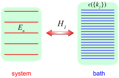
Figure 1: The energy spectra of the system and the heat bath. The spectral density of the heat bath should be much larger then the system.

We generally consider a composite coupled system, which can be divided into a system $S$ with Hamiltonian $H_{S}$ and a heat bath $B$ with Hamiltonian $H_{B}$. The coupling between the system and the bath can be generally described by $H_{I}$. Then we have the total Hamiltonian $H=H_{S}+H_{B}+H_{I}$. The system and the bath have the following spectrum decompositions

$$H_{S} = \sum_{n}E_{n}\left|n\right\rangle\left\langle n\right|,$$ (1)

$$H_{B} = \sum_{j=1}^{N}\sum_{k_{j}}\epsilon_{k_{j}}\left|k_{j}\right\rangle\left\langle k_{j}\right|.$$ (2)

Here, $\left|n\right\rangle$ is the eigenstate of the system with the corresponding eigen energy $E_{n}$. The heat bath is composed of $N$ identical particles, the eigenstate of the $j$th particle is $\left|k_{j}\right\rangle$ with the corresponding eigen energy $\epsilon_{k_{j}}$. Usually, the energy spectrum of the system is much sparser than the heat bath, i.e.,

$$|E_{n}-E_{m}|\gg|\epsilon(\{k_{j}\})-\epsilon(\{l_{j}\})|,$$ (3)

which holds for two arbitrary energy levels $n$ and $m$ of the system (see Fig. 1), and two arbitrary bath energy states configurations $\{k_{j}\}$ and $\{l_{j}\}$. Here, we denote $\epsilon(\{k_{j}\})=\sum_{\{k_{j}\}}\epsilon_{k_{j}}$.

The system-bath interaction $H_{I}$ is weak comparing to $H_{0}$, which generally reads

$$H_{I}=\sum_{j=1}^{N}\sum_{n,n^{\prime},k_{j},k_{j}^{\prime}}g_{nk_{j},n^{\prime}k_{j}^{\prime}}\left|nk_{j}\right\rangle\left\langle n^{\prime}k_{j}^{\prime}\right|$$ (4)

with $\left|nk_{j}\right\rangle\equiv\left|n\right\rangle\otimes\left|k_{j}\right\rangle$. Next we consider the role of the off-diagonal terms with respect to the system indexes $n$ in $H_{I}$. The first order perturbation effect of these off-diagonal terms with $n\neq n^{\prime}$ can be ignored under the condition

$$\Big{|}\frac{g_{nk_{j},n^{\prime}k_{j}^{\prime}}}{E_{n^{\prime}}-E_{n}+\epsilon_{k_{j}^{\prime}}-\epsilon_{k_{j}}}\Big{|}\ll 1,$$ (5)

However, for the terms with $n=n^{\prime}$, the above condition $\big{|}g_{nk_{j},nk_{j}^{\prime}}(\epsilon_{k_{j}^{\prime}}-\epsilon_{k_{j}})^{-1}\big{|}\ll 1$ will be violated due to the properties of the energy spectra given in Eq. (3). Thus the diagonal terms can contribute to the system behaviors and should be kept in the interaction Hamiltonian Dong2010 , which yields

$$H_{I}\approx\sum_{j=1}^{N}\sum_{n,k_{j},k_{j}^{\prime}}g_{nk_{j},nk_{j}^{\prime}}\left|nk_{j}\right\rangle\left\langle nk_{j}^{\prime}\right|.$$

Then, the total effective Hamiltonian has the diagonal form with respect to the eigenstates of the system, i.e.,

$$H_{\mbox{eff}}=\sum_{n}[E_{n}+h(n)]\left|n\right\rangle\left\langle n\right|$$ (6)

with

$$h(n)=\sum_{j=1}^{N}\sum_{k_{j},k_{j}^{\prime}}\left(\epsilon_{k_{j}}\delta_{k_{j},k_{j}^{\prime}}+g_{nk_{j},nk_{j}^{\prime}}\right)\left|k_{j}\right\rangle\left\langle k_{j}^{\prime}\right|.$$ (7)

Here, $h(n)$ describes the heat bath Hamiltonian corresponding to the system energy level $\left|n\right\rangle$. It can be further diagonalized as $h(n)=\sum_{j=1}^{N}\sum_{\alpha_{j}}\varepsilon_{\alpha_{j}}(n)\left|\alpha_{j}\right\rangle\left\langle\alpha_{j}\right|$. The new energy spectrum of the heat bath $\{\varepsilon_{\alpha_{j}}\}$ deforms comparing with the original energy spectrum $\{\epsilon_{k_{i}}\}$ due to the system-bath coupling. This system-bath coupling is usually negligible when we study the thermalized state of the system in a large heat bath. However, if the dimension of the heat bath is relatively small, i.e. the finite system thermodynamic case, this coupling has significant effect on modifying the canonical distribution of the system.

To derive the canonical distribution of the system in a large heat bath, it is usually assumed an energy shell between $E-E_{n}$ and $E-E_{n}+\delta$ in the phase space, where $E$ is the total energy of the system and heat bath, $\delta$ is the thickness of the energy shell which is a small quantity. This energy shell includes a set of states

$$V_{0}\left(E-E_{n}\right):\{\left|n,\{k_{i}\}\right\rangle|E-E_{n}\leq\sum_{\{k_{j}\}}\epsilon_{k_{j}}\leq E-E_{n}+\delta\}.$$ (8)

Here, the system-bath interaction energy is neglected and $V_{0}$ gives a constrain on the configurations of heat bath states $\left|\{k_{i}\}\right\rangle$ when the system energy is fixed at $E_{n}$. Then, according to the postulate that each microscopic state has an equal priori probability, the probability of the system in the state $\left|n\right\rangle$ is proportional to the number of states in $V_{0}\left(E-E_{n}\right)$,

$$P_{0}(E,E_{n})=\frac{\Omega(E-E_{n})}{W(E)},$$ (9)

where $\Omega(E-E_{n})$ denotes the number of states satisfying the constrain Eq.(8), and $W(E)=\sum_{n}\Omega(E-E_{n})$ Huang1987 .

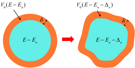
Figure 2: The energy shell without and with the consideration of the system-bath coupling, which shifts the energy shell for $\Delta_{n}$.

In the situation of finite system statistics, it is crucial to consider the system-bath interaction energy for the relatively small heat bath. The effective Hamiltonian Eq. (6) is already diagonalized with diagonal elements $E(n,\{\alpha_{i}\})=E_{n}+\sum_{\{\alpha_{i}\}}\varepsilon_{\alpha_{i}}(n)$. It explicitly defines an energy shell as the subspace $V\left(E-E_{n}\right)$:

$$\{\left|n,\{\alpha_{i}(n)\}\right\rangle|E-E_{n}\leq\sum_{\{\alpha_{i}\}}\varepsilon_{\alpha_{i}}(n)\leq E-E_{n}+\delta\}.$$ (10)

Nevertheless, it is more convenient to count the number of states in $V\left(E-E_{n}\right)$ via the bath bases $\{\left|k_{i}\right\rangle\}$. Because $V\left(E-E_{n}\right)$ is a geometrical deformed energy shell comparing with $V_{0}\left(E-E_{n}\right)$, we re-express it as $V_{0}\left(E-E_{n}-\Delta_{n}\right)$:

$$\{\left|n,\{\alpha_{i}(n)\}\right\rangle|E-E_{n}-\Delta_{n}\leq\sum_{\{k_{i}\}}\epsilon_{k_{i}}\leq E-E_{n}-\Delta_{n}+\delta\},$$ (11)

where the geometrical deformation of the energy shell is characterized by $\Delta_{n}=\sum_{\{\alpha_{i}\}}\varepsilon_{\alpha_{i}}(n)-\sum_{\{k_{i}\}}\epsilon_{k_{i}}$. The deformation of the energy shell is schematically illustrated in Fig. 2. By counting the number of states in $V_{0}\left(E-E_{n}-\Delta_{n}\right)$, we can obtain the probability of the the system in the state $\left|n\right\rangle$ as

$$P(E,E_{n})=\frac{\Omega(E-E_{n}-\Delta_{n})}{W(E)}.$$ (12)

Different from $P_{0}(E,E_{n})$ in Eq. (9), $P(E,E_{n})$ takes the system-bath coupling into account.

To further obtain the statistic distribution of the system, we introduce the entropy as $S(E)=k\ln\Omega(E)$, where $k$ is the Boltzmann constant. Usually, $E_{n}+\Delta(n)$ is much smaller than the total energy $E$, thus the entropy reads

$$S(E-E_{n}-\Delta_{n}) \approx S(E)-\frac{\partial S(E^{\prime})}{\partial E^{\prime}}\bigg{|}_{E^{\prime}=E}(E_{n}+\Delta_{n})$$ (13)

$$+\frac{\partial^{2}S(E^{\prime})}{\partial E^{\prime 2}}\bigg{|}_{E^{\prime}=E}\Delta_{n}E_{n}$$

The first term $S(E)$ is independent of $E_{n}$, thus it does not determine the specific distribution form. The derivative terms of $S(E)$ can be evaluated directly from its definition, as $\Omega(E)$ is proportional to the volume of the energy shell in the phase space. In a $N$-dimensional space, the volume confined in an isoenergic surface of energy $E$ can be considered as the volume of a $N$-dimensional polyhedron with effective radius $E$, which is proportional to $E^{\zeta N}$, here $\zeta$ is a dimensionless real number independent of $N$ and is usually related to the degeneracy of the system states. Therefore, the volume of the energy shell is given by

$$\Omega(E)\varpropto(E+\delta)^{\zeta N}-E^{\zeta N},$$ (14)

which leads to

$$\beta\left(E\right)=\frac{\partial S(E^{\prime})}{\partial E^{\prime}}\bigg{|}_{E^{\prime}=E}=\frac{k\left(\zeta N-1\right)}{E}.$$ (15)

With the thermodynamic relations, $\beta=(kT)^{-1}$ and $T$ is the temperature of the finite system in equilibrium. Obviously, Eq.(15) recovers the equipartition theorem $E\approx\zeta NkT$, i.e., each degree of freedom contributes $\zeta kT$ to the total energy. Therefore, the non-canonical statistic distribution function reads

$$P(E,E_{n}) = \frac{1}{\mathcal{Z}}e^{-\beta(E_{n}+\Delta_{n})+\xi\Delta_{n}E_{n}},$$ (16)

where $\mathcal{Z}=\sum\exp[-\beta(E_{n}+\Delta_{n})+\xi\Delta_{n}E_{n}]$ is the partition function with

$$\xi(E)=\frac{\partial^{2}S(E^{\prime})}{\partial E^{\prime 2}}\bigg{|}_{E^{\prime}=E}=-\frac{k\left(\zeta N-1\right)}{E^{2}}.$$ (17)

If the interaction energy could be neglected comparing with the total energy $E$, all the terms containing $\Delta_{n}$ in Eq. (16) can be dropped and thus naturally lead to the usual canonical statistics distribution function

$$P_{can}(E,E_{n}) = \frac{1}{\mathcal{Z}}\exp(-\beta E_{n}).$$ (18)

Otherwise, the deformation of energy shell $\Delta_{n}$ will shift the system energy level and thus modify the distribution function. We can sort the system eigenvalues in an ascending order with $E_{n+1}>E_{n}$ for any $n$. Accordingly, we assume the energy shell deformation $\Delta_{n}<0$ and $|\Delta_{n+1}|>|\Delta_{n}|$ (as illustrated by the general model below). It follows from Eqs.(16, 18) that

$$\frac{P(E,E_{n+1})}{P(E,E_{n})}>\frac{P_{can}(E,E_{n+1})}{P_{can}(E,E_{n})},$$ (19)

which means in the non-canonical statistics, the higher energy levels play more important role than that in the canonical statistics.

III illustration with harmonic oscillators system

Now we consider a coupled harmonic oscillators system as an example to illustrate the statistical thermodynamic properties of a finite system. The system $S$ is a single harmonic oscillator with eigenfrequency $\omega$ and $a^{\dagger}(a)$ as its creation (annihilation) operator. The heat bath is generally modeled as a collection of harmonic oscillators with Hamiltonian $H_{B}=\sum_{j=1}^{N}\omega_{j}b_{j}^{\dagger}b_{j}$. Here $b_{j}^{\dagger}(b_{j})$ is the creation (annihilation) operator of the oscillator with frequency $\omega_{j}$. In the weak coupling limit, we can assume the effective system-bath interaction as

$$H_{I}=\sum_{j=1}^{N}\lambda_{j}a^{\dagger}a(b_{j}^{\dagger}+b_{j}).$$ (20)

In this model, the eigenvalues of the total Hamiltonian are

$$E(n,\{m_{j}(n)\}) =n\omega+\Delta_{n}+\sum_{\{m_{j}\}}m_{j}\omega_{j},$$ (21)

which corresponding to the eigenstates $\left|n,\{m_{j}(n)\}\right\rangle=\left|n\right\rangle\otimes\prod_{j=1}^{N}\left|m_{j}(n)\right\rangle$. The eigenstate of the heat bath $\left|m_{j}(n)\right\rangle$ is defined as a displaced Fock state $\left|m_{j}(n)\right\rangle=D(-\lambda_{j}n/\omega_{j})\left|m_{j}\right\rangle$, with the displacement operator $D(\alpha_{j})=\exp(\alpha a_{j}^{\dagger}-\alpha^{\ast}a_{j})$. Here, the deformation of the energy shell is described by an $n$-dependent factor

$$\Delta_{n}=-\sum_{j=1}^{N}\frac{\lambda_{j}^{2}n^{2}}{\omega_{j}}\equiv-\kappa n^{2}.$$ (22)

Due to this deformation, the non-canonical distribution function with high order correction is given by

$$P(E,n\omega) = \frac{1}{\mathcal{Z}}e^{-\beta(n\omega-n^{2}\kappa)-\xi\omega\kappa n^{3}}.$$ (23)

The square and cubic terms of $n$ in the exponent of $P(E,n\omega)$ greatly change the statistical distribution from the canonical distribution $P_{n}=\mathcal{Z}^{-1}\exp(-\beta n\omega)$, especially for large $n$. However, Eq.(23) does not apply to very large $N$ for the following reason: the total energy $E$ of the system and the heat bath is conserved, and the heat bath energy should always be nonnegative $\sum_{\{m_{j}\}}m_{j}\omega_{j}>0$. Thus, the energy shell of Eq.(11) constrains the system energy level by $E\geq E_{n}$, which implies $n<(\omega-\sqrt{\omega^{2}-4\kappa E})/(2\kappa)$. Therefore, for such coupled finite system, the maximum energy level for the system is

$$n_{max}=\left\lfloor\frac{\omega-\sqrt{\omega^{2}-4\kappa E}}{2\kappa}\right\rfloor,$$ (24)

here $\left\lfloor x\right\rfloor$ represents the maximum integer below $x$.

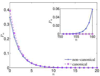
Figure 3: The non-canonical (blue solid line) and canonical (pink dashed line) distribution functions for coupled oscillators system. We choose $\omega=1$, $E=100$, $\beta=0.5$ and $\kappa=0.00235$. The highest energy level is $n_{max}=160$. The non-canonical and canonical distributions are similar for low energy levels while of great difference for high energy levels.

Usually $\kappa$ is much smaller than $\omega$, thus the non-canonical statistics distribution $P(E,n\omega)$ for low energy levels is not very different from the canonical one, as shown in Fig. 3. However, as $|\Delta_{n}|$ grows with $n^{2}$, the high energy levels share much more ratio than that in the canonical distribution, which can be seen from the inset of Fig. 3. We choose the system eigen frequency as unit $\omega=1$, the total energy $E=100$ and $\kappa=0.00235$. According to Eq.(24), the highest energy level is $n_{max}=160$ in this situation. The canonical distribution is plotted by set $\kappa=0$ in $P(E,n\omega)$. A numerical research also gave the similar non-canonical distribution for coupled spin systems WXZhang2010 .

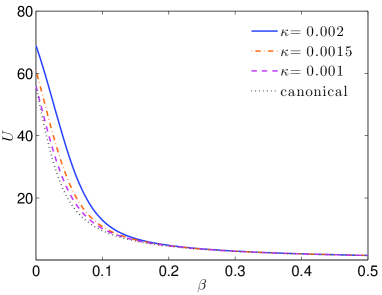
Figure 4: The internal energy $U$ of the system with respect to $\beta$ for non-canonical and canonical statistics. We plot the cases of $\kappa=0.002$, $n_{max}=138$ (blue solid line), $\kappa=0.0015$, $n_{max}=122$ (orange dotted-dash line), $\kappa=0.001$, $n_{max}=112$ (pink dashed line) and the canonical case for $\kappa=0$, $n_{max}=112$.

Because the high energy states have relatively larger populations, the internal energy of the system

$$U=\sum_{n=0}^{n_{max}}n\omega P(E,n\omega)$$ (25)

under the non-canonical statistics is larger than that under the canonical one. This fact is illustrated in Fig. 4, where the internal energy $U$ is plotted with respect to $\beta$. The distinction between the non-canonical and canonical statistics for $U$ evidently appears when the inverse temperature $\beta$ decreases and the interaction energy strength $\kappa$ grows. As $\beta$ approaches to zero, the high temperature limit of the internal energy $U$ arrives at $n_{max}\omega/2$, which is finite as the total energy is up-bounded by $E$ for small heat bath. This is very different from the case in the thermodynamic limit: the average energy of a harmonic oscillator which contacts with an infinite heat bath will diverge when $\beta$ decreases to zero.

Another feature reflecting the non-monotony of the non-canonical distribution is the relative fluctuation of the system internal energy

$$\left(\Delta U\right)^{2}=\frac{1}{U^{2}}\sum_{n=0}^{n_{max}}\left(n\omega-U\right)^{2}P(E,n\omega).$$ (26)

As shown in Fig. 5, at both low and high temperature limits, the non-canonical and canonical statistics for finite system present similar fluctuation behavior. To characterize these two limits, we consider the system as a harmonic oscillator with truncated energy levels (the highest energy level is labeled by $n_{max}$) under canonical statistics ($\kappa=0$), whose energy fluctuation is denoted as $(\Delta U_{C})^{2}$. It is analytically calculated that in the low temperature limits, the fluctuation $(\Delta U_{C})^{2}\approx\exp(\beta\omega)$ is exactly the same as the result when $n_{max}\rightarrow\infty$. Because the populations of the high energy levels decrease significantly in the low temperature, only the several low energy levels determine the thermodynamic behavior. In the high temperature limit, the energy fluctuation behaves as

$$(\Delta U_{C})^{2}\approx\frac{1}{3}+\frac{2}{3n_{max}}+\frac{n_{max}}{9}\beta,$$

which is a linear function of $\beta$. We remark here that the high temperature limit and thermodynamic limit cannot commute with each other, as

$$\lim_{n_{max}\rightarrow\infty}\lim_{\beta\rightarrow 0}(\Delta U_{C})^{2}=\frac{1}{3},$$

while

$$\lim_{\beta\rightarrow 0}\lim_{n_{max}\rightarrow\infty}(\Delta U_{C})^{2}=1.$$

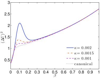
Figure 5: The internal energy relative fluctuation $(\Delta U)^{2}$ of the system with respect to $\beta$ for non-canonical and canonical statistics. The parameters are chosen the same as Fig. 4.

However, in the intermediate range of $\beta$, a local maximum in energy fluctuation distinguishes the non-canonical distribution from the canonical one, especially for strong system-bath interaction $\kappa$. This maximum can be qualitatively understood as follow: we can rewrite the non-canonical distribution as $P(E,n\omega)=\mathcal{Z}^{-1}\exp(-\beta\eta_{n}n\omega)$, where $\eta_{n}=1-\kappa n/\omega-\kappa n^{2}/E$ is a positive factor for $n\leq n_{max}$. As $\eta_{n}\leq 1$, the reverse temperature $\beta$ can be considered as effectively reduced by $\eta_{n}$, thus the linear region for small $\beta$ is enlarged in the non-canonical statistics. Based on the above observations, we know that the non-canonical statistics exhibits obviously novel effects when the interaction energy strength $\kappa$ is large and the temperature is high.

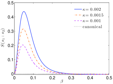
Figure 6: The mutual entropy of two identical harmonic oscillators (HOs) by non-canonical and canonical statistics. The eigen frequency of two identical HOs is $\omega=1$, and $\kappa=0.002$, $n_{max}=138$ (blue solid line), $\kappa=0.0015$, $n_{max}=122$ (orange dotted-dash line), $\kappa=0.001$, $n_{max}=112$ (pink dashed line) and the canonical case for $\kappa=0$, $n_{max}=112$.

Besides the high distribution tail for a single system, the non-canonical statistics provides other new characters when the system is composite of two independent subsystem $l_{1}$ and $l_{2}$. Even if these two subsystems do not directly interact with each other, the deformation of the energy shell can effectively result in correlation between them. Here we still use harmonic oscillator (HO) systems for illustration. The system consists of two single mode HOs with Hamiltonian $H_{S}=\sum_{k=1,2}\omega_{k}a_{k}^{\dagger}a_{k}$. The system interacts with a common small heat bath, which can be modeled by the Hamiltonian $H_{B}=\sum_{j=1}^{N}\omega_{j}b_{j}^{\dagger}b_{j}$. The interaction term reads

$$H_{I}=\sum_{k=1,2}\sum_{j=1}^{N}\lambda_{kj}a_{k}^{\dagger}a_{k}(b_{j}^{\dagger}+b_{j}).$$

Following the same discussion about the energy shell deformation for a single system, we can straightforwardly obtain the joint distribution of the composite system as

$$P(E,E_{n}^{(1)},E_{m}^{(2)}) = \frac{1}{\mathcal{Z}_{t}}e^{-\beta(E_{nm}+\Delta_{nm})+\xi\Delta_{nm}E_{nm}},$$ (27)

where $E_{nm}=n\omega_{1}+m\omega_{2}$ and

$$\Delta_{nm} = -\sum_{j=1}^{N}\frac{(\lambda_{1j}n+\lambda_{2j}m)^{2}}{\omega_{j}}$$

$$\mathcal{Z}_{t} = \sum_{n,m}\,^{\prime}e^{-\beta(E_{nm}+\Delta_{nm})+\xi\Delta_{nm}E_{nm}}.$$

Here $\sum_{n,m}^{\prime}$ means the summation of the system energy levels should satisfy the constrain $0\leq E_{nm}+\Delta_{nm}\leq E$. It can be seen from Eq.(27) that the statistics of two subsystems are not independent with each other due to the cross-term in $\Delta_{nm}$. This statistical correlation can be described by mutual information defined as

$$S(l_{1}:l_{2})=S(l_{1})+S(l_{2})-S(l_{1}+l_{2}),$$

where the entropy $S(l_{k})=-\sum_{n=0}^{n_{max}}P(E,E_{n}^{(k)})\ln P(E,E_{n}^{(k)})$ and $S(l_{1}+l_{2})=-\sum_{n,m}^{\prime}P(E,E_{n}^{(1)},E_{m}^{(2)})\ln P(E,E_{n}^{(1)},E_{m}^{(2)})$. For simplicity, we assume the two HOs are identical with $\omega_{1}=\omega_{2}\equiv\omega$, $\lambda_{1j}=\lambda_{2j}\equiv\lambda_{j}$ and $\kappa$ is defined the same as Eq.(22). As shown in Fig. 6, there appears a non-zero mutual entropy if we use non-canonical statistics to describe the composite system in a common small heat bath. In contrary, if the interaction energy is too small to be considered comparing with the total energy, we can use the canonical distribution to calculate the mutual entropy which naturally gives $S(l_{1}:l_{2})=0$, i.e., the two subsystems are not correlated with each other.

IV conclusion

We study the statistical thermodynamics of an open system whose interaction with the heat bath cannot be neglect. The interaction modifies the system energy shell and leads to the non-canonical statistical distribution for such system. It is shown that non-canonical distribution has a big “tail” for higher energy levels, which is the most significant difference from the canonical distribution. This non-canonical feature results in higher internal energy and energy fluctuation of the system. And different parts of the composite system are naturally correlated with each other which is described by mutual entropy. We would like to mention that the non-canonical form of distribution may be related to the explanation of black hole information paradox MSZhan .

This work is supported by National Natural Science under Grants No.11121403, No. 10935010, No. 11074261, No.11222430, No.11074305 and National 973 program under Grants No. 2012CB922104.

References

- (1) T. Kinoshita, T. Wenger, and D. S. Weiss, Nature (London) 440, 900 (2006).
- (2) J. Liphardt, S. Dumont, S. B. Smith, I. Tinoco Jr., C. Bustamante, Science 296, 1832 (2002).
- (3) T. L. Hill, J. Chem. Phys. 36, 3182 (1962).
- (4) H. Dong, S. Yang, X. F. Liu, and C. P. Sun, Phys. Rev. A 76, 044104 (2007).
- (5) M. Rigol, V. Dunjko, and M. Olshanii, Nature (London) 452, 854 (2008).
- (6) J. Rau, Phys. Rev. A 84, 012101 (2011).
- (7) H. Hasegawa, Phys. Rev. E 83, 021104 (2011).
- (8) H. Hasegawa, J. Math. Phys. 52, 123301 (2011).
- (9) M. Falcioni, D. Villamaina, A. Vulpiani, A. Puglisi, and A. Sarracino, Am. J. Phys. 79, 777 (2011).
- (10) W. G. Wang, Phys. Rev. E 86, 011115 (2012).
- (11) G. L. Barnes and M. E. Kellman, J. Chem. Phys. 139, 214108 (2013).
- (12) P. Bocchieri and A. Loinger, Phys. Rev. 114, 948 (1959).
- (13) H. Tasaki, Phys. Rev. Lett. 80, 1373 (1998).
- (14) S. Popescu, A. J. Short, and A. Winter, Nat. Phys. 2, 754 (2006).
- (15) S. Goldstein, J. L. Lebowitz, R. Tumulka, and N. Zanghì, Phys. Rev. Lett. 96, 050403 (2006).
- (16) H. Dong, X.F. Liu, and C. P. Sun, Chin. Sci. Bull. 55, 3256 (2010).
- (17) K. Huang, Statistical Mechanics, John Wiley & Sons (1987).
- (18) Wenxian Zhang, C. P. Sun, and Franco Nori, Phys. Rev. E 82, 041127 (2010).
- (19) B. Zhang, Q. Y, Cai, L. You, and M. S. Zhan, Phys. Lett. B 675, 98 (2009); B. Zhang, Q. Y, Cai, M. S. Zhan, and L. You, Ann. Phys. 326, 350 (2011).