Stripe to spot transition in a plant root hair initiation model

Abstract

A generalised Schnakenberg reaction-diffusion system with source and loss terms and a spatially dependent coefficient of the nonlinear term is studied both numerically and analytically in two spatial dimensions. The system has been proposed as a model of hair initiation in the epidermal cells of plant roots. Specifically the model captures the kinetics of a small G-protein ROP, which can occur in active and inactive forms, and whose activation is believed to be mediated by a gradient of the plant hormone auxin. Here the model is made more realistic with the inclusion of a transverse co-ordinate. Localised stripe-like solutions of active ROP occur for high enough total auxin concentration and lie on a complex bifurcation diagram of single and multi-pulse solutions. Transverse stability computations, confirmed by numerical simulation show that, apart from a boundary stripe, these 1D solutions typically undergo a transverse instability into spots. The spots so formed typically drift and undergo secondary instabilities such as spot replication. A novel 2D numerical continuation analysis is performed that shows the various stable hybrid spot-like states can coexist. The parameter values studied lead to a natural singularly perturbed, so-called semi-strong interaction regime. This scaling enables an analytical explanation of the initial instability, by describing the dispersion relation of a certain non-local eigenvalue problem. The analytical results are found to agree favourably with the numerics. Possible biological implications of the results are discussed.

1 Introduction

An earlier paper [4] by three of the present authors along with Grierson analysed a mathematical model first derived by Payne and Grierson [25] for a prototypical morphogenesis occurring at a sub-cellular level. Specifically, the model accounts for the kinetics of a family of small G-proteins known collectively as the rho-proteins of plants, or ROPs for short. The model is intended to describe the observed initiation of hair-like protrusions in the epidermal cells of the roots of the model plant Arabidopsis thaliana (see [11, 12] and other references in [4] for details). The hairs themselves are crucial for anchorage and for nutrient uptake, and when fully formed comprise the majority of the surface area of the plant. In wild type, a single hair is formed in each root hair cell, at a set distance about 20% of the way along the cell from its basal end (i.e. end closest to root tip). The formation of a single localised patch of activated ROP is the precursor for such a strong symmetry breaking in the cell and is triggered as a newly formed root hair cell reaches a critical length. At the same time, the overall concentration of the pre-eminent plant hormone auxin increases throughout the cell and, due to the nature of how it is actively pumped, there is a gradient of auxin from high concentrations at the basal end to lower at the apical. The effect of auxin is postulated to account for a spatially-dependent gradient of the activation of the ROP.

In [4] many features of the root hair initiation process were shown to be captured by the model. The spatial domain of the long, thin root-hair cell was approximated by a one-dimensional spatial domain with the diffusion of the activated ROP being much slower, accounting for the fact that this form is bound to the membrane whereas inactivated ROP is free to diffuse within the cell. In particular, it was found that for small cell lengths and low auxin concentrations the active ROP is confined to a boundary patch. There is then a critical threshold in length and/or auxin for which a single interior patch forms. This process is hysteretic, in that if auxin-levels were instantaneously decreased, the patch would remain. Moreover, if auxin or cell length are decreased too rapidly a second instability can occur, resulting in the formation of multiple-patch states. These states appear to capture the pattern of root hairs seen in several mutant varieties. The purpose of this paper is to see how those results survive in a more realistic geometry.

The model in question takes the form of a two-component reaction-diffusion (RD) system that can be written in dimensionless form as

$$U_{t}=\varepsilon^{2}\Delta_{s}U+\alpha(x)U^{2}V-U+\frac{1}{\tau\gamma}V\,,$$ (1.1a)

$$\tau V_{t}=D\Delta_{s}V-V+1-\tau\gamma\left(\alpha(x)U^{2}V-U\right)-\beta\gamma U\,.$$ (1.1b)

Fig. 1: Sketch of an idealised 3D RH cell, and cell membrane (densely dashed lines) projection onto a 2D rectangular domain. The longitudinal auxin gradient is shown (grey shade) as a consequence of in- (bold solid arrows) and out pump (dashed arrows) mechanisms; see [10, 11, 18]. Influx and efflux permeabilities are depicted by $P_{i}$ and $P_{e}$ arrows respectively; auxin symplastic pathway is indicated by bold arrows in the 3D RH cell. Switching fluctuation is represented by blank-cusp solid arrows in $\tilde{\Omega}$.

In dimensionless form the model is posed on a square $(x,y)\in\Omega\equiv[0,1]\times[0,1]$, which has been rescaled from a rectangular domain $\tilde{\Omega}\equiv[0,L_{x}]\times[0,L_{y}]$ with $L_{x}=20\mu m$ and aspect ratio $s=(L_{x}/L_{y})^{2}=5.5$, so that in (1.1) we have defined $\Delta_{s}\equiv\partial_{xx}+s\partial_{yy}$. From now onwards, this operator will be considered as such. The biochemical interaction this system models is for a ROP bounding on-and-off switching fluctuation, which is assumed to take place on the cell membrane (see [4, 25]), and RH cells are flanked by non-RH cells, from which no ROPs exchange have been reported, as far as we have knowledge. Thus, homogeneous Neumann boundary conditions are assumed everywhere. The quantities $U(x,y,t)$ and $V(x,y,t)$ represent concentrations of the membrane-bound active ROP and unbound inactive ROP respectively and $\alpha(x)$ represents a monotone decreasing gradient of auxin, which is assumed to be at steady state and to vary only in the $x$ direction. In particular, in this work we shall assume that

$$\alpha(x)=e^{-\nu x}\qquad\mbox{with}\quad\nu=1.5\,,$$

which can be thought of as the outcome of a steady leaky diffusion process within the cell. A sketch of an idealised 3D RH cell and its cell membrane projection onto $\tilde{\Omega}$ can be seen in Fig. 1. Other dimensionless parameters are defined in terms of original parameters via

$$\varepsilon^{2}\equiv\frac{D_{1}}{L_{x}^{2}(c+r)}\,,\qquad D\equiv\frac{D_{2}}{L_{x}^{2}k_{1}}\,,\qquad\tau\equiv\frac{c+r}{k_{1}}\,,\qquad\beta\equiv\frac{r}{k_{1}}\,,$$ (1.2a)

and the primary bifurcation parameter $$\gamma$$ in this system is given by

$$\gamma\equiv\frac{(c+r)k_{1}^{2}}{k_{2}b^{2}}\,.$$ (1.2b)

Here $D_{1}\ll D_{2}$ are the diffusion constants for $U$ and $V$ respectively, $b$ is the rate of production of inactive ROP, $c$ is the rate constant for deactivation, $r$ is the rate constant describing active ROPs being used up in cell wall softening and subsequent hair formation, and the active activation step is assumed to be proportional to $k_{1}V+k_{2}\alpha(x)U^{2}V$. The activation and overall auxin level within the cell, which is autocatalytic acceleration induced by auxins, is represented by $k_{1}$ and $k_{2}$ respectively. The latter parameter plays an important role in some numerical investigations here, due to gathering the main biological hypothesis in the model. See [4, 25] for more details.

The results in [4] concern a 1D domain in which $s=\infty$ and the 2D Laplacian is replaced by $d^{2}/dx^{2}$. In this paper we shall extend the 1D analysis of [4] to study patterns in 2D. By trivially extending the 1D localised spikes, in the transverse direction, a localised stripe pattern is obtained. Our main goal is to study whether these stripe patterns are stable to 2D transverse perturbations, and to shed light on any secondary instabilities that occur. In particular we would like to see the extent to which a single interior circular patch of ROP is the preferred solution for sufficiently high auxin concentration, as this would be a more accurate description of the biological process we seek to describe.

Spatially homogeneous RD systems similar to (1.1), but without the spatial inhomogeneity, have been studied extensively by a number of authors. In 2D domains, patterns such as spots and stripes have been found both numerically and analytically and their dynamics uncovered. In particular the so-called Gierer–Meinhardt system [8, 13, 20] admits a wide collection of spot and stripe patterns. Richer dynamics that also include spot oscillations, snaking-bifurcation diagrams, and even spatiotemporal chaos can occur for the so-called BVAM system [1] and the Gray–Scott system [23, 24] among others. Such RD systems arise as descriptions of pigmentation patterns on the skin of fish and as models of other chemical and biological pattern formation systems (see for example the book by Murray [22] for an overview).

In a similar singularly perturbed limit, Doelman & van der Ploeg [7] and Kolokolnikov & Ward [16] have undertaken a theoretical analysis of the transverse stability of an interior localised stripe for the Gierer–Meinhardt model (for a similar analysis for the Gray–Scott model see [17, 21]). A novel feature of the present work is to adapt these analyses to the case of a model with a spatial gradient, and to extend the analysis to include boundary stripes.

Our study of (1.1) relies on a combination of numerical and analytical methodologies. Firstly, time-dependent numerical simulations of the PDE system together with numerical computations of the eigenvalue problem associated with transverse perturbations are used to show that, generally, interior or boundary stripes are unstable to transverse perturbations. This instability leads to the formation of localised spots. Our numerical results show that the spots drift in the direction of the auxin gradient, and can undergo a secondary instability of spot self-replication. Numerical bifurcation techniques in 2D are then used to compute intricate bifurcation diagrams associated with steady-state spot patterns, stripe patterns, and mixed-states consisting of a stripe and spots.

The outline of the paper is outlined as follows. In §2 we perform full numerical simulations and detailed numerical bifurcation analyses using parameter set one in Table 1. In addition, we numerically compute dispersion relations for several scenarios. Then, in §3 we perform further simulations revealing a plethora of patterns, similar to those that have been observed in time-dependent shape changing domains for other RD systems, see e.g. [26]. In the singularly perturbed limit $\varepsilon\to 0$, in §4 a non-local eigenvalue problem (NLEP) is derived and analyzed in order to determine theoretical properties of the dispersion relation associated with the transverse stability of both an interior and a boundary stripe. The analytical results from this stability theory are found to agree favourably with results from numerical simulations. Finally, in §5, some concluding remarks are given, including possible biological interpretations of our results, and suggestions for further work are given.

Parameter set:
	One		Two		Three
Original	Re-scaled	Original	Re-scaled	Original	Re-scaled
$D_{1}=0.1$	$\varepsilon^{2}=3.6\times 10^{-4}$	$D_{1}=0.1$	$\varepsilon^{2}=2.3\times 10^{-5}$	$D_{1}=0.075$	$\varepsilon^{2}=1.02\times 10^{-4}$
$D_{2}=10$	$D=0.4$	$D_{2}=50$	$D=0.5$	$D_{2}=20$	$D=0.51$
$k_{1}=0.01$	$\tau=11$	$k_{1}=0.01$	$\tau=44$	$k_{1}=0.008$	$\tau=18.75$
$b=0.01$	$\beta=1$	$b=0.005$	$\beta=4$	$b=0.008$	$\beta=6.25$
$c=0.1$		$c=0.4$		$c=0.1$
$r=0.01$		$r=0.04$		$r=0.05$
$k_{2}\in[0.01,1.0]$	$\gamma\in[11,0.11]$	$k_{2}\in[0.045,40]$	$\gamma\in[39.1,0.04]$	$k_{2}\in[10^{-3},2.934]$	$\gamma\in[150,0.051]$
$L_{x}=50$		$L_{x}=100$		$L_{x}=70$
$L_{y}=20$	$s=6.25$			$L_{y}=29.848$	$s=5.5$

Table 1: Three parameter sets in the original and dimensionless re-scaled variables. The fundamental units of length and time are $\mu\textrm{m}$ and sec, and concentration rates are measured by an arbitrary datum (con) per time unit; $k_{2}$ is measured by $\textrm{con}^{2}/\textrm{s}$, and diffusion coefficients units are $\mu\textrm{m}/\textrm{s}^{2}$.

2 Numerical investigation

We first present numerical computations that show stripe instabilities for the ROP model (1.1) with parameter set one given in Table 1, which are equivalent to those used in [25]. In terms of the operator $\Delta_{s}\equiv\partial_{xx}+s\partial_{yy}$ where $s=(L_{x}/L_{y})^{2}$ as is defined in §1, we recast (1.1) as

$$\partial_{t}\begin{bmatrix}U\\ V\end{bmatrix}=\mathbf{D}\begin{bmatrix}\Delta_{s}&0\\ 0&\Delta_{s}\end{bmatrix}\begin{bmatrix}U\\ V\end{bmatrix}+\begin{bmatrix}f(U,V,x)\\ g(U,V,x)\end{bmatrix},\quad(x,y)\in\Omega\,;\qquad\nabla_{\mathbf{n}}U=\nabla_{\mathbf{n}}V=0\,,\quad(x,y)\in\partial\Omega\,.$$ (2.3)

Here $\mathbf{D}$ is a diagonal diffusion matrix, $\mathbf{n}$ is the normal to $\partial\Omega$ at $(x,y)$ and where we have omitted the dependence on control parameters for simplicity. We present two types of computation: time-dependent simulation of (2.3) and numerical continuation of the corresponding steady states. Implementation details are given in §2.3.

2.1 Simulations

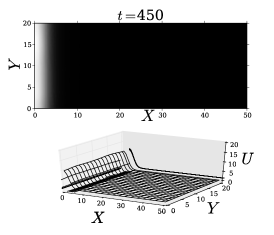
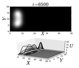
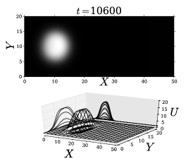
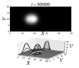
Fig. 2: Snapshots of a travelling front breaking up into a slowly travelling spot that gets pinned after a long time. (a) Front formed at the boundary. (b) Breakup into a peanut-shaped form. (c) Travelling spot. (d) Final pinned spot. Original parameter set one as given in Table 1 with $k_{2}=0.1$. Notice that the spot drifts very slowly in time.

As initial conditions for our time-dependent computations, we take a small random perturbation to

$$U_{0}\equiv\frac{1}{\gamma\beta}\,,\qquad V_{0}\equiv\frac{\tau\beta\gamma}{\tau+\beta^{2}\gamma}\,,$$

which is an equilibrium to the homogeneous problem with $\alpha(x)\equiv 1$. As shown below, the monotonically decreasing auxin gradient $\alpha(x)$, which is largest at $x=0$, has a strong influence on the dynamics. For $k_{2}=0.1$, full numerical results of the solution at different times are shown in Fig. 2. As time increases, a front is formed at the boundary. This front, resembling a boundary stripe (see Fig. 2), then travels towards the right where the auxin gradient is smaller. The stripe breaks up into a transitory “peanut-shape” [23] (see Fig. 2), which then slowly drifts towards the right boundary. The spot ultimately gets pinned at some distance from the right boundary, as shown in Fig. 2. From this simulation, as similarly observed in the 1D case in [4], there exists a separation of spatial and temporal scales. There are two spatial scales, one local and one global, for the $U$-concentration. Moreover, there is one time-scale associated with the quick destabilization of the boundary stripe into a spot, referred to as a breakup instability, and a second much longer time-scale associated with the slowly drifting spot. Although some aspects of the spatio-temporal scales are inherited from the 1D case analyzed in [4], the 1D theory cannot capture the stripe breakup nor the formation, drift, and pinning of the localised spot.

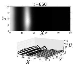
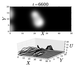
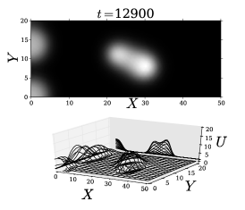
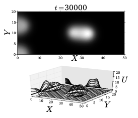
Fig. 3: Snapshots of two stripes breaking up into an asymmetrical array of spots. (a) Early localised stripes. (b)-(c) Stripes breaking apart, counterclockwise rotation and travelling peanut-form. (d) A pinned spot-like pattern. Original parameter set one as given in Table 1 with $k_{2}=0.4$.

To investigate how the bifurcation parameter $k_{2}$ affects the dynamics we increase this parameter to $k_{2}=0.4$. The initial conditions for the time-dependent computations are the same as above for $k_{2}=0.1$. The numerical results at different times are shown in Fig. 3. In Fig. 3 a stripe-like state is formed at the boundary, with a second stripe quickly emerging further towards the interior. Then, as these structures move away from each other, both stripes break up into two half-spots at the boundary and a counter-clockwise rotating peanut form, as shown in Figures 3–3. This structure then aligns itself longitudinally and drifts slowly towards the right (see Fig. 3).

In other singularly perturbed RD systems, localised structures can exist in regions where the nonlinear terms dominate (cf. [31]). In addition, since the system (1.1) is somewhat similar in form to both the Schnakenberg and Brusselator systems, we expect that both spot and self-replicating spot patterns can occur (cf. [15] and [28]). The 2D simulations shown above suggest that $\mathcal{O}(1)$ time-scale instabilities are associated with the formation of localised spots from a stripe. This type of breakup instability is analysed mathematically in §4 in a particular asymptotic limit.

2.2 Bifurcation diagram for stripes

To gain further insight into the existence and stability of stripes, we perform a numerical bifurcation analysis of stripe solutions using $k_{2}$ as the main bifurcation parameter. Stripes are stationary solutions $(u_{s}(x;y),v_{s}(x;y))^{T}$ to (2.3) that are constant in $y$. Hence, they satisfy the 1D boundary-value problem

$$\mathbf{D}\begin{bmatrix}\partial_{xx}&0\\ 0&\partial_{xx}\end{bmatrix}\begin{bmatrix}u_{s}\\ v_{s}\end{bmatrix}+\begin{bmatrix}f(u_{s},v_{s},x)\\ g(u_{s},v_{s},x)\end{bmatrix}=0\,,\quad x\in(0,1)\,;\qquad\partial_{x}u_{s}=\partial_{x}v_{s}=0\,,\qquad x=0,1\,.$$ (2.4)

To see this, notice that a parametric exploration of the 1D problem was performed previously (see Fig. 6 in [4]) and solutions to the 1D system can be trivially extended in $y$. In other words, let $(u_{s}(x),v_{s}(x))^{T}$ a steady solution of (2.4), in such fashion that extended solutions $(u_{s}(x;y),v_{s}(x;y))^{T}=(u_{s}(x),v_{s}(x))^{T}$, where $y$ is seen as a parameter providing the trivial extension. Which implies that $u_{s}(x;y)$ and $v_{s}(x;y)$ are also solutions of (2.4). Therefore, the bifurcation diagram of such solutions is entirely equivalent to Fig. 6 in [4]. However, the stability properties become dependent on perturbations in the $y$-direction. This can be seen as follows. We introduce

$$\tilde{U}=u_{s}+e^{\lambda t+imy}\varphi(x)\,,\qquad\tilde{V}=v_{s}+e^{\lambda t+imy}\psi(x)\,,$$ (2.5)

where $\varphi,\psi\ll 1$. The wavenumber $m$ is determined by the homogeneous Neumann boundary conditions at $y=0,1$. We thus require $m=k\pi$ for $k\in\mathbb{Z}$, and the perturbation takes the form $\Re(e^{imy})=\cos\left(k\pi y\right)$. Upon substituting (2.5) into (2.3), we obtain the eigenvalue problem

$$\lambda\begin{bmatrix}\varphi\\ \psi\end{bmatrix}=\begin{bmatrix}\varepsilon^{2}\partial_{xx}-sm^{2}+f_{U}(u_{s},v_{s},x)&f_{V}(u_{s},v_{s},x)\\ g_{U}(u_{s},v_{s},x)&(D/\tau)\partial_{xx}-sm^{2}+g_{V}(u_{s},v_{s},x)\end{bmatrix}\begin{bmatrix}\varphi\\ \psi\end{bmatrix}\,.$$ (2.6)

Thus, we compute stripes numerically as solutions to (2.4) and then study their linear stability by solving (2.6).

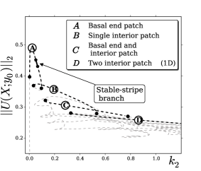
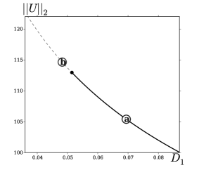
Fig. 4: (a) Comparison of bifurcation diagrams between localised stripes and 1D-spike scenarios. Bold dashed portions of the diagram indicate where stable 1D solutions are unstable to transverse instabilities. A narrow stable window is found, given by the solid black curve. (b) Bifurcation diagram as $D_{1}$ varies from a solution in stable-stripe branch shown in (a); $k_{2}=0.0463$. An eigenvalue crosses into the right-hand complex semi-plane at the filled black circle. Branch labelled by a remains stable as $D_{1}$ is increased further (not shown). Original parameter set one as given in Table 1.

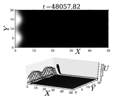
Fig. 5: Relevant snapshots of transversal instability for unstable boundary stripe b in Fig. 4. (a) Break up instability and (b) two newly formed boundary spots travelling towards interior. Original parameter set one as given in Table 1 with $k_{2}=0.0463$ and $D_{1}=0.0492$.

For the original parameter set one as given in Table 1, the bifurcation diagram for stripes is depicted in Fig. 4. We use the $L_{2}$-norm of the active component $U$ for a fixed value of $y$ as a solution measure. We find patterns with one boundary stripe (A), one interior stripe (B), one boundary and one interior stripe (C), and two interior stripes (D). All the solution branches, apart from a small segment (bold line), are unstable. Even so, as $\varepsilon^{2}$ is directly proportional to $D_{1}$, the stable extended pattern branch (solid black curve ends in Fig. 4) becomes unstable as $D_{1}$ decreases. Even though the nature of this instability will be analysed thoroughly in §4, this gives an insight on the asymptotic limit, i.e. sharper boundary stripes are unstable. To shed light on this, upon selecting a solution from the stable stripe-branch as initial condition, we perform continuation on $D_{1}$. As can be seen in Fig. 4, there is a small critical value at which boundary stripe solutions become unstable. In addition, we run a time-step simulation upon taking an unstable boundary stripe solution (labelled by b) as the initial condition. This computation shows the triggering of a break-up instability, which then gives rise to two spots moving towards domain interior. In Fig. 5 we give pertinent snapshots where the boundary stripe disintegrating into spots can be seen, as well as spot dynamics for short times. The transition from a boundary stripe to spot formation occurs on an $\mathcal{O}(1)$ time-scale as is similarly shown in Fig. 2 and Fig. 3. This confirms that 1D localised patterns tend to destabilise under transverse perturbations.

Moreover, the stability boundaries of the stable stripe-branch are symmetry-breaking pitchfork (Turing) bifurcation points, characteristic of a transition between one and three solutions as the bifurcation parameter crosses a critical value (cf. [9]). To motivate why these instabilities should occur in spite of the fact that the location of the boundary stripe does not vary with $k_{2}$, nor is there any gradient in the $y$-direction, one effectively finds that transverse instabilities are inherited from the 1D homogeneous problem. This homogeneous problem is readily analysed and one finds Turing instabilities as $k_{2}$ varies (see [3] for more details). Summarising these numerical results, we have:

Result 2.1.

System (1.1) is stripe-unstable under transverse perturbations. In addition, there exists two pitchfork bifurcation points that define a small stable boundary-stripe branch, which vanishes as $D_{1}$ decreases.

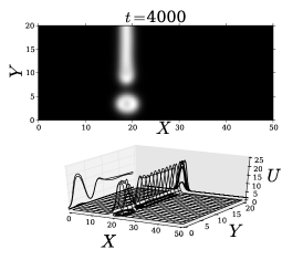
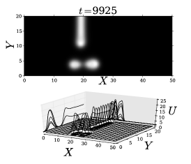
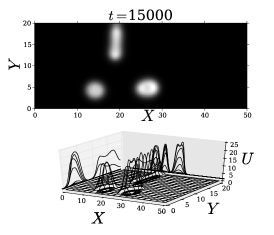
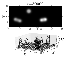
Fig. 6: Example of a breakup instability of an interior localised stripe into one spot and two peanut-forms. (a) The stripe breaks up into a semi-localised stripe and a spot. (b) Spot splits up. (c) Breakup of the semi-localised stripe into a peanut-form, and spots move away from each other. (d) A spot and two peanut-forms are finally formed. Original parameter set one as given in Table 1 with $D_{1}=0.025$ and $k_{2}=0.15$, which corresponds to a stripe location in $x_{0}=18.5$.

To gain further insight into the type of instability for stripes, we take an interior localised stripe as initial condition and perform a time-dependent simulation of the full PDE system. The results are shown in Fig. 6. We observe that first the stripe breaks up into a spot and a “semi-stripe” set at the initial location (Fig. 6). Then, the newly formed spot splits (Fig. 6) giving way to two small droplets. These two spots move away from other each while the semi-stripe collapses into a peanut form (Fig. 6). Finally, a spot is formed from the semi-stripe in addition to the two peanut-forms (see Fig. 6). Here two different instabilities are present: a breakup instability, which destabilizes the localised stripe to form spots, and another instability that creates peanut forms from spots. We will investigate breakup instabilities from a numerical viewpoint in §3.

2.3 Numerical Implementation

To time-step and compute steady states of (2.3), we introduce a regular grid $\{(x_{i},y_{j})\}$ of $N_{x}N_{y}$ nodes covering $\Omega\cup\partial\Omega$ and form vectors $\mathbf{U}=\{U(x_{i},y_{j})\}$ and $\mathbf{V}=\{V(x_{i},y_{j})\}$. The Laplacian operator $\Delta$ is approximated using second-order finite differences by forming explicitly differentiation matrices $\mathbf{D_{xx}}\in\mathbf{R}^{Nx\times Nx}$, $\mathbf{D_{yy}}\in\mathbf{R}^{Ny\times Ny}$ for second derivatives in $x$ and $y$, respectively, and combining them using Kronecker products, $\mathbf{L}=\mathbf{D_{xx}}\otimes\mathbf{I_{y}}+\mathbf{I_{x}}\otimes\mathbf{D_{yy}},$ where $\mathbf{I_{x}}$ and $\mathbf{I_{y}}$ are $N_{x}$-by-$N_{x}$ and $N_{y}$-by-$N_{y}$ identity matrices, respectively. We remark that the sparse discrete Laplacian $\mathbf{L}$ incorporates boundary conditions directly in the differentiation matrices. For the initial-boundary value problem, we set $N_{x}=N_{y}=60$, or $N_{x}=N_{y}=125$ and time-step the resulting discretized system of $2N_{x}N_{y}$ nonlinear ODEs

$$\dot{\mathbf{W}}=\mathbf{D}\otimes\begin{bmatrix}\mathbf{L}&0\\ 0&\mathbf{L}\end{bmatrix}\mathbf{W}+\begin{bmatrix}\mathbf{f}\left(\mathbf{W},\mathbf{x}\right)\\ \mathbf{g}\left(\mathbf{W},\mathbf{x}\right)\end{bmatrix},\qquad\mathbf{W}=(\mathbf{U},\mathbf{V})^{T}\,,$$

with a second order adaptive time stepper (Matlab in-built ode23s, to which we provide the Jacobian matrix explicitly). In our computations, the components of $\mathbf{U}$ and $\mathbf{V}$ are interleaved to minimise the Jacobian matrix bandwidth. We continue steady states as solutions to the discretised boundary-value problem

$$\mathbf{D}\otimes\begin{bmatrix}\mathbf{L}&0\\ 0&\mathbf{L}\end{bmatrix}\mathbf{W}+\begin{bmatrix}\mathbf{f}\left(\mathbf{W},\mathbf{x}\right)\\ \mathbf{g}\left(\mathbf{W},\mathbf{x}\right)\end{bmatrix}=\mathbf{0}\,,$$

using the Matlab function fsolve with the default tolerance and the secant continuation code developed in [27]. The linear stability property of steady states is determined by computing (a subset of) eigenvalues and eigenvectors of the Jacobian matrix of the discretised linear operator in (2.6) for stripes. In 2D calculations, we compute the five eigenvalues with the largest real part using the Matlab function eigs, whereas for stripes we determine the full spectrum with eig.

3 Stripes into spots

The numerical bifurcation analysis, initially depicted in Fig. 4, shows that solution branches, arising from the 1D analysis of [4], are generally not stable stable under transverse perturbations. This feature will be theoretically analyzed further in §4. Indeed, further computations below in Fig. 13 and Fig. 15 show that stripes are susceptible to breakup instabilities leading to spot formation.

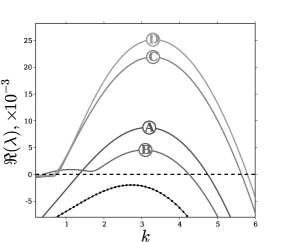
Fig. 7: Dispersion relations computed numerically for particular steady solutions marked in bifurcation diagram in Fig. 4; stable boundary stripe (dot-dashed line), (A) unstable boundary stripe, (B) single interior stripe, boundary and (C) interior stripe, and (D) two interior stripes. The dotted dispersion relation corresponds to a boundary stable solution. Original parameter set one as given in Table 1.

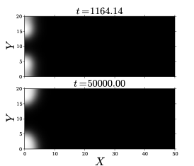
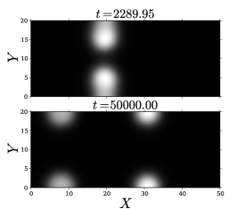
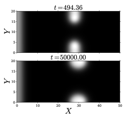
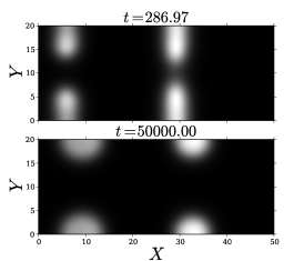
Fig. 8: Breakup instability (top panel) and final stable state solution (bottom panel) of each extended-solution kind: (a) boundary stripe, (b) an interior stripe, (c) boundary and interior stripe, and (d) two interior stripes. Original parameter set one as given in Table 1.

In order to verify that unstable solutions in Fig. 4 exhibit breakup, leading to spot formation, we choose a solution from each branch, and respectively compute its dispersion relation. In Fig. 7 each curve is labelled accordingly to solution kind (see also labels in Fig. 4): (A) unstable boundary stripe, (B) an interior stripe, (C) boundary and interior stripe, and (D) two interior stripes. The dispersion relation for a stable boundary solution is computed, which is shown by a dotted curve. Upon using each of these steady-states as initial conditions and performing a direct time-step computation, we confirm that those labelled from (A) up to (D) are indeed unstable, while the solution corresponding to the dotted curve is stable. Fig. 8 shows the initial creation of spots induced by breakup instabilities (top panels) and the final stable states (bottom panels). Although, according to the dispersion relations in Fig. 7, the most unstable mode should theoretically predict the number of spots the stripe should break up into, the prediction from Fig. 7 is seen to provide an over-estimate of the number of spots that are seen in the computations. This results from the choice of the parameter set one in Table 1, where $\varepsilon$ is not too small. Consequently any spots created from a breakup instability are rather “fat” and not significantly localised. Nevertheless, it is clear from these computations that $\mathcal{O}(1)$ time-scale instabilities play an important role in destabilising stripes. We remark that, for a different parameter set with a smaller $\varepsilon$ leading to more localised spots, in §4 we will obtain a more quantitatively favorable comparison between the theoretical prediction of the number of spots arising from a breakup instability and that observed in full numerical simulations (see Fig. 13 and Fig. 15 below).

In addition to breakup instabilities of a stripe, a secondary ${\mathcal{O}}(1)$ time-scale instability of spot self-replication can also occur. This instability is evident in the transition observed in Fig. 8. From this figure, we observe that once spots are formed from a breakup instability, there is a further self-replication instability in which each spot splits into two small droplets near the upper and lower boundary. The ultimate location of these droplets is transversally determined by the auxin gradient, which induces a slow drift of the droplets to their eventual steady-state locations. A further interesting feature shown in Fig. 8, is that it is possible that only the interior stripe undergoes a breakup instability while the boundary stripe remains intact. This shows that a steady-state pattern consisting of both spots and stripes can occur at the same parameter value.

3.1 A richer zoo

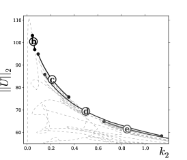
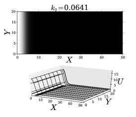
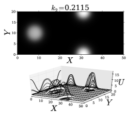
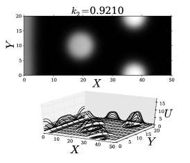
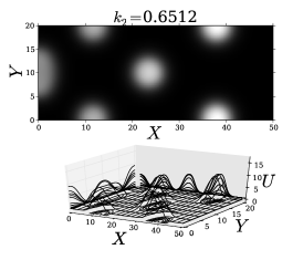
Fig. 9: Bifurcation diagram: spots and a boundary stripe. (a) Stable branches are drawn by solid lines and unstable ones by light-grey dashed lines, and filled circles represent fold points. Stable solutions, accordingly to labels (b) up to (e), are shown in: (b) a boundary stripe, (c) a spot in the interior and two spots at the boundary, (d) a boundary stripe, an interior spot and two spots at the boundary, and (e) an interior spot and five spots at the boundary. Original parameter set one as given in Table 1.

The lower panels of Fig. 8 suggest that a wide variety of mixed spot and stripe patterns can be created through breakup instabilities. In order to explore these new types of solution further, we shall perform full numerical continuation of 2D solutions. To do this, we begin with a solution on the stable steady-state branch of Fig. 4. We then continue this solution by varying the main bifurcation parameter $k_{2}$, both backwards and forwards, to finally obtain the bifurcation diagram depicted in Fig. 9. There, all unstable branches are plotted as light-grey dashed lines, whereas stable branches are represented as solid lines labelled accordingly as: (b) stable stripes, (c) an interior spot and two spots vertically aligned at the boundary, (d) similar configuration but with an additional stripe, and (e) an interior spot and five spots at the boundary. See Figures 9–9 for examples of each stable steady-state. In Fig. 9, as seen before, the bifurcation diagram replicates features studied in the 1D case in  [4], such as the overlapping of stable branches of single and multiple localised patches. Stable branches typically become unstable through fold bifurcations. All branches seem to lie on a single connected curve, and no other bifurcations were found except for the pitchfork bifurcations in branch (b). However, branches (c) up to (e) are extremely close to each other and apparently inherit properties from each other. That is, they seem to undergo a creation-annihilation cascade effect similar to that observed in [4]. In other words, take a steady-state which lies on the left-hand end of branch (c) and slide down this branch as $k_{2}$ is increased. It then loses stability at the fold point, and at the other extreme to then fall off in branch (d). Thus a stripe emerges, which pushes the interior spot further in. The same transition follows up to branch (e), more spots arise though as the stripe is destroyed. No further stable branches with steady-states resembling either spots or stripes were found.

4 Breakup instabilities of localised stripes

In [7] and [14] a theoretical framework for the stability analysis of a localised stripe for the Gierer–Meinhardt reaction-diffusion system was given. This previous analysis is not directly applicable to the ROP problem (1.1) owing to the presence of the spatially dependent coefficient $\alpha(x)$ that modulates the nonlinear term. In the limit $\varepsilon\to 0$, in this section we extend the analysis of [14] to theoretically explain the breakup instability of stripe solutions numerically observed in Fig. 5 and Fig. 6.

We first re-scale variables in (1.1) by $U=\varepsilon^{-1}u$ and $V=\varepsilon v$ and we assume $D={\mathcal{O}}(\varepsilon^{-1})$ so that $D=\varepsilon^{-1}D_{0}$ with $D_{0}={\mathcal{O}}(1)$ (see [4]). Then, (1.1) becomes

$$u_{t}=\varepsilon^{2}\left(u_{xx}+su_{yy}\right)+\alpha(x)u^{2}v-u+\frac{\varepsilon^{2}}{\tau\gamma}v\,,$$ (4.7a)

$$\varepsilon\tau v_{t}=D_{0}\left(v_{xx}+sv_{yy}\right)+1-\varepsilon v-\varepsilon^{-1}\left[\tau\gamma\left(\alpha(x)u^{2}v-u\right)+\beta\gamma u\right]\,,$$ (4.7b)

with homogeneous Neumann boundary conditions at $x=0,1$ and $y=0,1$. The relation between the dimensionless parameters $\tau$, $\gamma$, $\beta$, and $D_{0}$ and the original parameters is given above in (1.2).

4.1 An Interior Stripe

We first consider the stability of an isolated, interior localised stripe. To do so, we first need to construct for $\varepsilon\to 0$ a 1D quasi steady-state spike solution centred at some $x_{0}$ in $0<x_{0}<1$. From Proposition 4.1 of [4], this spike solution for (4.7) has the leading-order asymptotics

$$u_{s}\sim\frac{1}{\alpha(x_{0})v^{0}}w\left[\varepsilon^{-1}(x-x_{0})\right]\,,\qquad w(\xi)\equiv\frac{3}{2}\textnormal{sech}^{2}\left({\xi/2}\right)\,,$$ (4.8a)

$$v_{s}\sim v^{0}-\frac{\left(x-x_{0}\right)^{2}}{2D_{0}}+\frac{1}{D_{0}}\left\{\begin{array}[]{ll}-x_{0}\left(x-x_{0}\right)\,,&0\leq x\leq x_{0}\,,\\ \\ \left(1-x_{0}\right)\left(x-x_{0}\right),&x_{0}<x\leq 1\,,\end{array}\right.\,,\qquad v^{0}\equiv\frac{6\beta\gamma}{\alpha\left(x_{0}\right)}\,.$$ (4.8e)

Here $w(\xi)$ is the unique homoclinic orbit of $w^{\prime\prime}-w+w^{2}=0$ with $w(0)>0$, $w^{\prime}(0)=0$, and $w\to 0$ as $|\xi|\to\infty$.

We extend this solution trivially in the $y$-direction to form a stripe. To determine the stability of this stripe solution we introduce the transverse perturbation of (4.8) in the same form as in (2.5). Upon substituting this perturbation into (4.7), we get the following singularly perturbed eigenvalue problem with $\varphi_{x}=\psi_{x}=0$ at $x=0,1$:

$$\varepsilon^{2}\varphi_{xx}-\varphi+2\alpha(x)u_{s}v_{s}\varphi+\alpha(x)u_{s}^{2}\psi+\frac{\varepsilon^{2}}{\tau\gamma}\psi=\left(\lambda+s\varepsilon^{2}m^{2}\right)\varphi\,,$$ (4.9a)

$$D_{0}\left(\psi_{xx}-sm^{2}\psi\right)-\varepsilon^{-1}\tau\gamma\alpha(x)u_{s}^{2}\psi-\varepsilon\psi=\varepsilon^{-1}\left[\tau\gamma\left(2\alpha(x)u_{s}v_{s}\varphi-\varphi\right)+\beta\gamma\varphi\right]+\varepsilon\tau\lambda\psi\,.$$ (4.9b)

There are two distinct classes of eigenvalues for (4.9), each giving rise to a different type of instability (see [14]). The small eigenvalues, with $\lambda={\mathcal{O}}(\varepsilon^{2})$, govern zigzag instabilities, whereas the large eigenvalues with $\lambda={\mathcal{O}}(1)$ as $\varepsilon\to 0$ govern the linear stability of the amplitude of the stripe. For the Gierer–Meinhardt model, this latter instability was found in [14] to be the mechanism through which a nonlinear event is triggered leading to the break up of the stripe into localised spots. The simulations and numerical analysis in §2 suggest that breakup instabilities dominate on an ${\mathcal{O}}(1)$ time-scale, and hence we shall only focus on analysing the large eigenvalues with $\lambda={\mathcal{O}}(1)$ as $\varepsilon\to 0$.

To analyse such breakup instabilities, we must derive an NLEP from (4.9). Since the time-evolution of a 1D quasi steady-state spike centred at $x_{0}$ moves at an ${\mathcal{O}}(\varepsilon^{2})\ll 1$ speed (see [4]), in our stability analysis of the ${\mathcal{O}}(1)$ eigenvalues we will consider $x_{0}$ to be frozen. The steady-state solution for $x_{0}$ is characterized by Proposition 4.3 of [4].

We begin by looking for a localised eigenfunction for $\varphi(x)$ in the form

$$\Phi(\xi)=\varphi(x_{0}+\varepsilon\xi)\,,\qquad\xi\equiv\varepsilon^{-1}(x-x_{0})\,,\qquad\Phi\to 0\,\quad\mbox{as}\quad|\xi|\to\infty\,.$$ (4.10)

We then use (4.8) to calculate $2u_{s}v_{s}\alpha\sim 2w$ and $\alpha u_{s}^{2}\sim{\alpha(x_{0})w^{2}/\left[\alpha(x_{0})v^{0}\right]^{2}}$ for $x$ near $x_{0}$. In this way, we obtain from (4.9a) that $\Phi(\xi)\sim\Phi_{0}(\xi)+o(1)$, where $\Phi_{0}$ satisfies

$${\mathcal{L}}_{0}\Phi_{0}+\frac{w^{2}}{\alpha(x_{0})\left[v^{0}\right]^{2}}\psi(x_{0})=\left(\lambda+s\varepsilon^{2}m^{2}\right)\Phi_{0}\,,\quad-\infty<\xi<\infty\,;\qquad\Phi_{0}\to 0\,\quad\mbox{as}\quad|\xi|\to\infty\,.$$ (4.11)

Here ${\mathcal{L}}_{0}\Phi_{0}\equiv\Phi_{0\xi\xi}-\Phi_{0}+2w\Phi_{0}$ is referred to as the local operator.

Next, we must calculate $\psi(x_{0})$ in (4.11) from (4.9b). Since $u_{s}$ and $\varphi$ are localised, we use (4.8) to calculate as $\varepsilon\to 0$ the coefficients in (4.9b) in the sense of distributions as

$$\varepsilon^{-1}\tau\gamma\alpha(x)u_{s}^{2}\psi\longrightarrow\frac{\tau\gamma}{\alpha(x_{0})\left[v^{0}\right]^{2}}\left[\int_{-\infty}^{\infty}w^{2}\,d\xi\right]\psi(x)\,\updelta(x-x_{0})\,,$$

$$\varepsilon^{-1}\left[\tau\gamma\left(2\alpha(x)u_{s}v_{s}\varphi-\varphi\right)+\beta\gamma\varphi\right]\longrightarrow 2\tau\gamma\left[\int_{-\infty}^{\infty}\left(w\Phi_{0}-\kappa\Phi_{0}\right)\,d\xi\right]\,\updelta(x-x_{0})\,,\qquad\kappa\equiv\frac{1}{2}\left(1-\frac{\beta}{\tau}\right)\,,$$

where $\int_{-\infty}^{\infty}w^{2}\,d\xi=6$. Similar calculations for the 1D spike were given in (5.4) of [4]. In this way, we obtain from (4.9b) that, in the outer region, $\psi\sim\psi_{0}$ where $\psi_{0}$ satisfies

$$D_{0}\left(\psi_{0xx}-sm^{2}\psi_{0}\right) -\frac{6\tau\gamma}{\alpha(x_{0})\left[v^{0}\right]^{2}}\psi_{0}(x)\updelta(x-x_{0})=2\tau\gamma\left[\int_{-\infty}^{\infty}\left(w\Phi_{0}-\kappa\Phi_{0}\right)\,d\xi\right]\,\updelta\left(x-x_{0}\right)\,,$$ (4.12)

with $\psi_{0x}=0$ at $x=0,1$. This problem for $\psi_{0}$ is equivalent to the following problem with jump conditions across $x=x_{0}$:

$$\left\{\begin{array}[]{l}\psi_{0xx}-sm^{2}\psi_{0}=0,\qquad 0<x<x_{0}\,,\quad x_{0}<x<1\,;\qquad\psi_{0x}\left(0\right)=\psi_{0x}\left(1\right)=0\,,\\ \left[\psi_{0}\right]_{x_{0}}=0\,,\quad D_{0}\left[\psi_{0x}\right]_{x_{0}}=\frac{\displaystyle a_{0}}{\displaystyle\gamma}\psi_{0}(x_{0})+\gamma b_{0}\,,\end{array}\right.$$ (4.15)

where we define the bracket notation as $\left[z\right]_{x_{0}}\equiv z(x_{0}^{+})-z(x_{0}^{-})$. In (4.15), we have defined $a_{0}$ and $b_{0}$ by

$$a_{0}\equiv\frac{6\tau\gamma^{2}}{\alpha\left(x_{0}\right)\left[v^{0}\right]^{2}}\,,\qquad b_{0}\equiv 2\tau\int\limits_{-\infty}^{\infty}\left(w\Phi_{0}-\kappa\Phi_{0}\right)\,d\xi\,,\qquad\kappa\equiv\frac{1}{2}\left(1-\frac{\beta}{\tau}\right)\,.$$ (4.16)

To represent the solution to (4.15) we introduce the Green’s function $G\left(x;x_{0}\right)$ satisfying

$$G_{xx}-sm^{2}G=-\updelta\left(x-x_{0}\right)\,,\quad 0<x<1\,;\qquad G_{x}(0;x_{0})=G_{x}(1;x_{0})=0\,;\qquad\left[G_{x}\right]_{x_{0}}=-1\,.$$ (4.17)

For existence of this $G$ we require that $m>0$. The case $m=0$, studied in [4], corresponds to the stability problem of a 1D spike and requires the introduction of the modified or Neumann Green’s function. Here we consider the case $m>0$. For $m>0$, the solution to (4.15) is $\psi(x)=AG\left(x;x_{0}\right)$, where $A$ is determined from the jump condition in (4.15). In this way, we calculate $\psi(x_{0})$ as

$$\psi_{0}(x_{0})=-\frac{\gamma^{2}b_{0}}{a_{0}G^{0}+\gamma D_{0}}G^{0}\,,\qquad G^{0}\equiv G(x_{0};x_{0})\,.$$ (4.18)

Upon substituting (4.18) into (4.11), and from the definitions of $a_{0}$ and $b_{0}$ in (4.16), we obtain that

$${\mathcal{L}}_{0}\Phi_{0}-2\chi w^{2}\left(\frac{G^{0}}{D_{0}+6\chi G^{0}}\right)\int_{-\infty}^{\infty}\left(w\Phi_{0}-\kappa\Phi_{0}\right)\,d\xi=\left(\lambda+s\varepsilon^{2}m^{2}\right)\Phi_{0}\,,$$ (4.19)

where we have defined $\chi$ by

$$\chi\equiv\displaystyle\frac{\tau\gamma}{\alpha\left(x_{0}\right)\left[v^{0}\right]^{2}}\,,\qquad v^{0}=\frac{6\beta\gamma}{\alpha(x_{0})}\,.$$

Next, we introduce a parameter $\mu$ defined by

$$\mu\equiv\frac{12\chi G^{0}}{D_{0}+6\chi G^{0}}=2\left(1+\frac{D_{0}}{6\chi G^{0}}\right)^{-1}\,.$$ (4.20)

In terms of this parameter, (4.19) becomes

$${\mathcal{L}}_{0}\Phi_{0}-\frac{\mu}{6}w^{2}\left(I_{1}-\kappa I_{2}\right)=\left(\lambda+s\varepsilon^{2}m^{2}\right)\Phi_{0}\,,$$ (4.21)

where $I_{1}$, and $I_{2}$, are defined by $I_{1}\equiv\int_{-\infty}^{\infty}w\Phi_{0}\,d\xi$ and $I_{2}\equiv\int_{-\infty}^{\infty}\Phi_{0}\,d\xi$.

The NLEP (4.21) involves two non-local terms. To derive an NLEP in a more standard form with only one nonlocal term, we integrate (4.21) from $-\infty<\xi<\infty$ to relate $I_{1}$ and $I_{2}$ as

$$I_{2}=\frac{2-\mu}{\lambda+1+s\varepsilon^{2}m^{2}-\mu\kappa}I_{1}\,,$$ (4.22)

where we have used $\int_{-\infty}^{\infty}w^{2}\>d\xi=6$. Then, upon using this relation to eliminate $I_{2}$ in (4.21) we obtain an NLEP characterizing breakup instabilities for an interior localised stripe. We summarize our result in the following formal proposition:

Proposition 4.1.

The stability on an ${\mathcal{O}}(1)$ time-scale of a quasi steady-state interior stripe solution of (4.7) is determined by the spectrum of the NLEP

$${\mathcal{L}}_{0}\Phi_{0}-\theta_{h}(\lambda;m)\,w^{2}\>\frac{\int_{-\infty}^{\infty}w\Phi_{0}\>d\xi}{\int_{-\infty}^{\infty}w^{2}\,d\xi}=\left(\lambda+s\varepsilon^{2}m^{2}\right)\Phi_{0}\,,\quad-\infty<\xi<\infty\,;\quad\Phi_{0}\to 0\,,\quad\mbox{as}\quad|\xi|\to\infty\,,$$ (4.23a)

where $${\mathcal{L}}_{0}\Phi_{0}\equiv\Phi_{0\xi\xi}-\Phi_{0}+2w\Phi_{0} \theta_{h}(\lambda;m)$$, and is given by

$$\theta_{h}(\lambda;m)\equiv\mu\left(\frac{\lambda+1+s\varepsilon^{2}m^{2}-2\kappa}{\lambda+1+s\varepsilon^{2}m^{2}-\mu\kappa}\right)\,,$$ (4.23b)

$$\mu\equiv 2\left(1+\frac{D_{0}}{6\chi G^{0}}\right)^{-1}\,,\qquad\chi\equiv\displaystyle\frac{\tau\alpha\left(x_{0}\right)}{36\beta^{2}\gamma}\,,\qquad G^{0}\equiv G\left(x_{0};x_{0}\right)\,.$$

Here $G\left(x;x_{0}\right)$ is defined by (4.17), and the wavenumber $m$ in the $y$-direction is $m=k\pi$ with $k\in\mathbb{Z}^{+}$.

The NLEP (4.23a) is not self-adjoint, it has a nonlocal term and the multiplier $\theta_{h}$ depends on $\lambda$. However, our goal is to prove the following proposition:

Proposition 4.2.

The NLEP in (4.23) has a unique unstable eigenvalue when $m$ lies within an instability band $0<m_{\textrm{\em low}}<m<m_{\textrm{\em up}}$, with $m_{\textrm{\em low}}={\mathcal{O}}(1)$ and $m_{\textrm{\em up}}={\mathcal{O}}\left(\varepsilon^{-1}\right)$.

The spectrum of the NLEP is shown to be similar to that sketched in Fig. 10 (see also Fig. 7). The upper edge of the band $m_{\textrm{up}}$ will depend on the aspect ratio $s$. The expected number of spots that are predicted to form from the break up of the stripe can be estimated from the maximum growth rate $m^{*}$ in Fig. 10.

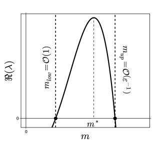
Fig. 10: Sketch of a dispersion relation $\Re(\lambda)$ versus $m$, showing the unstable band of wavenumbers lying between the vertical dashed lines. The expected number of spots is closely determined by the most unstable mode $m^{*}$.

To prove Proposition 4.2, we first need to determine the edges of the band of instability. To do so, we derive a few detailed properties of the Green’s function satisfying (4.17), as provided in the following lemma.

Lemma 4.1.

Define $G^{0}\equiv G(x_{0};x_{0})$ where $G(x;x_{0})$ satisfies (4.17). Then,

$$G^{0}\sim\frac{1}{sm^{2}}\,\quad\mbox{as}\quad m\to 0^{+}\,;\qquad G^{0}\sim\frac{1}{2\mathchoice{{\hbox{$\displaystyle\sqrt{s\,}$}\lower 0.4pt\hbox{\vrule height=4.30554pt,depth=-3.44446pt}}}{{\hbox{$\textstyle\sqrt{s\,}$}\lower 0.4pt\hbox{\vrule height=4.30554pt,depth=-3.44446pt}}}{{\hbox{$\scriptstyle\sqrt{s\,}$}\lower 0.4pt\hbox{\vrule height=3.01389pt,depth=-2.41113pt}}}{{\hbox{$\scriptscriptstyle\sqrt{s\,}$}\lower 0.4pt\hbox{\vrule height=2.15277pt,depth=-1.72223pt}}}m}\,\quad\mbox{as}\quad m\to\infty\,,$$ (4.24a)

$$\frac{dG^{0}}{dm}<0\,,\quad\mbox{for}\quad m>0\,;\qquad\frac{dG^{0}}{dx_{0}}>0\,,\quad\mbox{for}\quad 0<x_{0}<{1/2}\,,\quad m>0\,.$$ (4.24b)

• From (4.17), we readily calculate that

  $$G\left(x;x_{0}\right)=\frac{1}{\mathchoice{{\hbox{$\displaystyle\sqrt{s\,}$}\lower 0.4pt\hbox{\vrule height=4.30554pt,depth=-3.44446pt}}}{{\hbox{$\textstyle\sqrt{s\,}$}\lower 0.4pt\hbox{\vrule height=4.30554pt,depth=-3.44446pt}}}{{\hbox{$\scriptstyle\sqrt{s\,}$}\lower 0.4pt\hbox{\vrule height=3.01389pt,depth=-2.41113pt}}}{{\hbox{$\scriptscriptstyle\sqrt{s\,}$}\lower 0.4pt\hbox{\vrule height=2.15277pt,depth=-1.72223pt}}}m\sinh\left(\mathchoice{{\hbox{$\displaystyle\sqrt{s\,}$}\lower 0.4pt\hbox{\vrule height=4.30554pt,depth=-3.44446pt}}}{{\hbox{$\textstyle\sqrt{s\,}$}\lower 0.4pt\hbox{\vrule height=4.30554pt,depth=-3.44446pt}}}{{\hbox{$\scriptstyle\sqrt{s\,}$}\lower 0.4pt\hbox{\vrule height=3.01389pt,depth=-2.41113pt}}}{{\hbox{$\scriptscriptstyle\sqrt{s\,}$}\lower 0.4pt\hbox{\vrule height=2.15277pt,depth=-1.72223pt}}}m\right)}\left\{\begin{array}[]{lr}\cosh\left(\mathchoice{{\hbox{$\displaystyle\sqrt{s\,}$}\lower 0.4pt\hbox{\vrule height=4.30554pt,depth=-3.44446pt}}}{{\hbox{$\textstyle\sqrt{s\,}$}\lower 0.4pt\hbox{\vrule height=4.30554pt,depth=-3.44446pt}}}{{\hbox{$\scriptstyle\sqrt{s\,}$}\lower 0.4pt\hbox{\vrule height=3.01389pt,depth=-2.41113pt}}}{{\hbox{$\scriptscriptstyle\sqrt{s\,}$}\lower 0.4pt\hbox{\vrule height=2.15277pt,depth=-1.72223pt}}}mx\right)\cosh\left(\mathchoice{{\hbox{$\displaystyle\sqrt{s\,}$}\lower 0.4pt\hbox{\vrule height=4.30554pt,depth=-3.44446pt}}}{{\hbox{$\textstyle\sqrt{s\,}$}\lower 0.4pt\hbox{\vrule height=4.30554pt,depth=-3.44446pt}}}{{\hbox{$\scriptstyle\sqrt{s\,}$}\lower 0.4pt\hbox{\vrule height=3.01389pt,depth=-2.41113pt}}}{{\hbox{$\scriptscriptstyle\sqrt{s\,}$}\lower 0.4pt\hbox{\vrule height=2.15277pt,depth=-1.72223pt}}}m\left(1-x_{0}\right)\right)\,,&\quad 0\leq x<x_{0}\\ \cosh\left(\mathchoice{{\hbox{$\displaystyle\sqrt{s\,}$}\lower 0.4pt\hbox{\vrule height=4.30554pt,depth=-3.44446pt}}}{{\hbox{$\textstyle\sqrt{s\,}$}\lower 0.4pt\hbox{\vrule height=4.30554pt,depth=-3.44446pt}}}{{\hbox{$\scriptstyle\sqrt{s\,}$}\lower 0.4pt\hbox{\vrule height=3.01389pt,depth=-2.41113pt}}}{{\hbox{$\scriptscriptstyle\sqrt{s\,}$}\lower 0.4pt\hbox{\vrule height=2.15277pt,depth=-1.72223pt}}}mx_{0}\right)\cosh\left(\mathchoice{{\hbox{$\displaystyle\sqrt{s\,}$}\lower 0.4pt\hbox{\vrule height=4.30554pt,depth=-3.44446pt}}}{{\hbox{$\textstyle\sqrt{s\,}$}\lower 0.4pt\hbox{\vrule height=4.30554pt,depth=-3.44446pt}}}{{\hbox{$\scriptstyle\sqrt{s\,}$}\lower 0.4pt\hbox{\vrule height=3.01389pt,depth=-2.41113pt}}}{{\hbox{$\scriptscriptstyle\sqrt{s\,}$}\lower 0.4pt\hbox{\vrule height=2.15277pt,depth=-1.72223pt}}}m\left(1-x\right)\right)\,,&\quad x_{0}<x\leq 1\end{array}\right.\,,$$

  which determines $G^{0}$ as

  $$G^{0}=\frac{\cosh\left(\mathchoice{{\hbox{$\displaystyle\sqrt{s\,}$}\lower 0.4pt\hbox{\vrule height=4.30554pt,depth=-3.44446pt}}}{{\hbox{$\textstyle\sqrt{s\,}$}\lower 0.4pt\hbox{\vrule height=4.30554pt,depth=-3.44446pt}}}{{\hbox{$\scriptstyle\sqrt{s\,}$}\lower 0.4pt\hbox{\vrule height=3.01389pt,depth=-2.41113pt}}}{{\hbox{$\scriptscriptstyle\sqrt{s\,}$}\lower 0.4pt\hbox{\vrule height=2.15277pt,depth=-1.72223pt}}}mx_{0}\right)\cosh\left(\mathchoice{{\hbox{$\displaystyle\sqrt{s\,}$}\lower 0.4pt\hbox{\vrule height=4.30554pt,depth=-3.44446pt}}}{{\hbox{$\textstyle\sqrt{s\,}$}\lower 0.4pt\hbox{\vrule height=4.30554pt,depth=-3.44446pt}}}{{\hbox{$\scriptstyle\sqrt{s\,}$}\lower 0.4pt\hbox{\vrule height=3.01389pt,depth=-2.41113pt}}}{{\hbox{$\scriptscriptstyle\sqrt{s\,}$}\lower 0.4pt\hbox{\vrule height=2.15277pt,depth=-1.72223pt}}}m\left(1-x_{0}\right)\right)}{\mathchoice{{\hbox{$\displaystyle\sqrt{s\,}$}\lower 0.4pt\hbox{\vrule height=4.30554pt,depth=-3.44446pt}}}{{\hbox{$\textstyle\sqrt{s\,}$}\lower 0.4pt\hbox{\vrule height=4.30554pt,depth=-3.44446pt}}}{{\hbox{$\scriptstyle\sqrt{s\,}$}\lower 0.4pt\hbox{\vrule height=3.01389pt,depth=-2.41113pt}}}{{\hbox{$\scriptscriptstyle\sqrt{s\,}$}\lower 0.4pt\hbox{\vrule height=2.15277pt,depth=-1.72223pt}}}m\sinh\left(\mathchoice{{\hbox{$\displaystyle\sqrt{s\,}$}\lower 0.4pt\hbox{\vrule height=4.30554pt,depth=-3.44446pt}}}{{\hbox{$\textstyle\sqrt{s\,}$}\lower 0.4pt\hbox{\vrule height=4.30554pt,depth=-3.44446pt}}}{{\hbox{$\scriptstyle\sqrt{s\,}$}\lower 0.4pt\hbox{\vrule height=3.01389pt,depth=-2.41113pt}}}{{\hbox{$\scriptscriptstyle\sqrt{s\,}$}\lower 0.4pt\hbox{\vrule height=2.15277pt,depth=-1.72223pt}}}m\right)}\,.$$ (4.25)

  Upon expanding the hyperbolic functions for small and large argument we readily obtain the asymptotics in (4.24a) for $m\to 0$ and $m\to\infty$. To determine ${dG^{0}/dx_{0}}$, we differentiate (4.25) to get

  $$\frac{dG^{0}}{dx_{0}}=\frac{\sinh\left[\mathchoice{{\hbox{$\displaystyle\sqrt{s\,}$}\lower 0.4pt\hbox{\vrule height=4.30554pt,depth=-3.44446pt}}}{{\hbox{$\textstyle\sqrt{s\,}$}\lower 0.4pt\hbox{\vrule height=4.30554pt,depth=-3.44446pt}}}{{\hbox{$\scriptstyle\sqrt{s\,}$}\lower 0.4pt\hbox{\vrule height=3.01389pt,depth=-2.41113pt}}}{{\hbox{$\scriptscriptstyle\sqrt{s\,}$}\lower 0.4pt\hbox{\vrule height=2.15277pt,depth=-1.72223pt}}}m(2x_{0}-1)\right]}{\sinh(\mathchoice{{\hbox{$\displaystyle\sqrt{s\,}$}\lower 0.4pt\hbox{\vrule height=4.30554pt,depth=-3.44446pt}}}{{\hbox{$\textstyle\sqrt{s\,}$}\lower 0.4pt\hbox{\vrule height=4.30554pt,depth=-3.44446pt}}}{{\hbox{$\scriptstyle\sqrt{s\,}$}\lower 0.4pt\hbox{\vrule height=3.01389pt,depth=-2.41113pt}}}{{\hbox{$\scriptscriptstyle\sqrt{s\,}$}\lower 0.4pt\hbox{\vrule height=2.15277pt,depth=-1.72223pt}}}m)}>0\,,\quad\mbox{for}\quad 0<x_{0}<{1/2}\,.$$

  To prove the final statement in (4.24) we proceed indirectly. We define the self-adjoint operator $L$ by $Lu\equiv u_{xx}-sm^{2}u$, and differentiate (4.17) with respect to $m$ to get $L\left({dG/dm}\right)=2smG$. Then, from Lagrange’s identify, we derive

  $$0=\int_{0}^{1}\left[GL\left(\frac{dG}{dm}\right)-\frac{dG}{dm}LG\right]\,dx=2sm\int_{0}^{1}G^{2}\,dx+\int_{0}^{1}\frac{dG}{dm}\delta(x-x_{0})\,dx=2sm\int_{0}^{1}G^{2}\,dx+\frac{dG^{0}}{dm}\,.$$

  Therefore, ${dG^{0}/dm}=-2sm\int_{0}^{1}G^{2}\,dx<0$ for $m>0$, which completes the proof of (4.24). $\blacksquare$

To determine the upper edge of the instability band we use $G^{0}={\mathcal{O}}({1/m})$ as $m\to\infty$, to conclude that $\theta_{h}={\mathcal{O}}({1/m})$ in (4.23b). Therefore, for $m\gg 1$, the effect of the nonlocal term in the NLEP is asymptotically insignificant. With this observation, we let $m={m_{0}/\varepsilon}$, with $m_{0}={\mathcal{O}}(1)$ in (4.23a) to obtain, in terms of ${\mathcal{L}}_{0}\Phi_{0}\equiv\Phi_{0\xi\xi}-\Phi_{0}+2w\Phi_{0}$, that

$$\mathcal{L}_{0}\Phi_{0}-{\mathcal{O}}(\varepsilon)=\left(\lambda+sm_{0}^{2}\right)\Phi_{0}\,.$$ (4.26)

It is well-known (see [19]), that the local eigenvalue problem $\mathcal{L}_{0}\Psi=\upnu\Psi$ with $\Psi\to 0$ as $|\xi|\to\infty$ has a unique positive eigenvalue $\upnu_{0}={5/4}$ with positive eigenfunction $\Psi_{0}=\textnormal{sech}^{3}\left({\xi/2}\right)$. With this identification, (4.26) shows that $\lambda=\upnu_{0}-sm_{0}^{2}+{\mathcal{O}}(\varepsilon)$, so that $\lambda<0$ if $m_{0}>\mathchoice{{\hbox{$\displaystyle\sqrt{\upnu_{0}/s\,}$}\lower 0.4pt\hbox{\vrule height=7.5pt,depth=-6.00003pt}}}{{\hbox{$\textstyle\sqrt{\upnu_{0}/s\,}$}\lower 0.4pt\hbox{\vrule height=7.5pt,depth=-6.00003pt}}}{{\hbox{$\scriptstyle\sqrt{\upnu_{0}/s\,}$}\lower 0.4pt\hbox{\vrule height=5.25pt,depth=-4.20003pt}}}{{\hbox{$\scriptscriptstyle\sqrt{\upnu_{0}/s\,}$}\lower 0.4pt\hbox{\vrule height=3.75pt,depth=-3.00002pt}}}$ and $\lambda>0$ if $m_{0}<\mathchoice{{\hbox{$\displaystyle\sqrt{\upnu_{0}/s\,}$}\lower 0.4pt\hbox{\vrule height=7.5pt,depth=-6.00003pt}}}{{\hbox{$\textstyle\sqrt{\upnu_{0}/s\,}$}\lower 0.4pt\hbox{\vrule height=7.5pt,depth=-6.00003pt}}}{{\hbox{$\scriptstyle\sqrt{\upnu_{0}/s\,}$}\lower 0.4pt\hbox{\vrule height=5.25pt,depth=-4.20003pt}}}{{\hbox{$\scriptscriptstyle\sqrt{\upnu_{0}/s\,}$}\lower 0.4pt\hbox{\vrule height=3.75pt,depth=-3.00002pt}}}$. Upon setting $\lambda=0$, we obtain the upper edge of the instability band of the interior stripe in terms of both the dimensional variables and the original variables of (1.2) as

$$m_{\textrm{up}}\sim\frac{1}{\varepsilon}\mathchoice{{\hbox{$\displaystyle\sqrt{\frac{\upnu_{0}}{s}\,}$}\lower 0.4pt\hbox{\vrule height=8.26276pt,depth=-6.61024pt}}}{{\hbox{$\textstyle\sqrt{\frac{\upnu_{0}}{s}\,}$}\lower 0.4pt\hbox{\vrule height=5.80971pt,depth=-4.6478pt}}}{{\hbox{$\scriptstyle\sqrt{\frac{\upnu_{0}}{s}\,}$}\lower 0.4pt\hbox{\vrule height=4.51804pt,depth=-3.61446pt}}}{{\hbox{$\scriptscriptstyle\sqrt{\frac{\upnu_{0}}{s}\,}$}\lower 0.4pt\hbox{\vrule height=4.51804pt,depth=-3.61446pt}}}\,,\quad\upnu_{0}={5/4}\,;\qquad m_{\textrm{up}}\sim\mathchoice{{\hbox{$\displaystyle\sqrt{\frac{\upnu_{0}(c+r)}{D_{1}}\,}$}\lower 0.4pt\hbox{\vrule height=14.31888pt,depth=-11.45515pt}}}{{\hbox{$\textstyle\sqrt{\frac{\upnu_{0}(c+r)}{D_{1}}\,}$}\lower 0.4pt\hbox{\vrule height=10.0361pt,depth=-8.02892pt}}}{{\hbox{$\scriptstyle\sqrt{\frac{\upnu_{0}(c+r)}{D_{1}}\,}$}\lower 0.4pt\hbox{\vrule height=7.39165pt,depth=-5.91335pt}}}{{\hbox{$\scriptscriptstyle\sqrt{\frac{\upnu_{0}(c+r)}{D_{1}}\,}$}\lower 0.4pt\hbox{\vrule height=7.39165pt,depth=-5.91335pt}}}L_{y}\,.$$ (4.27)

Next, to estimate the lower threshold $m_{\textrm{low}}$, we suppose that $m\ll{\mathcal{O}}(\varepsilon^{-1})$, so that we neglect the $s\varepsilon^{2}m^{2}$ terms in (4.23b) to leading order. Then, we obtain that $\theta_{h}(\lambda;m)=\theta_{h0}(\lambda;m)+{\mathcal{O}}(\varepsilon^{2}m^{2})$, where

$$\theta_{h0}(\lambda;m)\equiv\mu\left(\frac{\lambda+1-2\kappa}{\lambda+1-\mu\kappa}\right)\,,$$ (4.28)

and $\mu$ is defined in (4.23b). Now as $m\to 0$, we have $G^{0}\to\infty$ from (4.24a), so that $\mu\to 2$. Therefore, $\theta_{h0}(\lambda;m)\to 2>1$ as $m\to 0$ for all $\lambda$. We conclude from Lemma A and Theorem 1.3 of [30] that a 1D spike is stable on an ${\mathcal{O}}(1)$ time-scale for any choice of the parameters $\beta$, $\tau$, and $\gamma$. From the analysis in §3 of [29] based on the rigorous study of the NLEP in [30], we obtain that an instability occurs at mode number $m$ whenever

$$\theta_{h0}\left(0;m\right)=\mu\left(\frac{1-2\kappa}{1-\mu\kappa}\right)<1\,.$$ (4.29)

This sufficient condition for instability is examined further in Proposition 4.3 below. To prove that (4.29) has a unique root, we differentiate (4.29) with respect to $m$ to obtain

$$\frac{d\theta_{h0}\left(0;m\right)}{dm}=\left[\frac{(1-2\kappa)}{(1-\mu\kappa)}+\frac{\mu\kappa(1-2\kappa)}{(1-\mu\kappa)^{2}}\right]\frac{d\mu}{dm}\,.$$ (4.30)

From the definition of $\mu$ in (4.23b), and from the properties of $G^{0}$ in Lemma 4.1, we have that $\mu\to 2$ as $m\to 0$, with $\mu<2$ and ${d\mu/dm}<0$ for $m>0$. Moreover, since $\kappa={\left(1-{\beta/\tau}\right)/2}<{1/2}$, we obtain that $(1-\mu\kappa)>0$ in (4.30). Therefore, we conclude from (4.30) that ${d\theta_{h0}\left(0;m\right)/dm}<0$ with $\theta_{h0}\left(0;m\right)\to 2$ as $m\to 0$ and $\theta_{h0}\left(0;m\right)={\mathcal{O}}(1/m)$ for $m\gg 1$. This proves that there is a unique value $m_{0\textrm{low}}$ of $m$ for which $\theta_{h0}\left(0;m\right)=1$. By using (4.29) and (4.23b) for $\theta_{h0}$ and $\mu$, respectively, we get that $\theta_{h0}\left(0;m\right)=1$ when $m=m_{0\textrm{low}}$, where $m_{0\textrm{low}}$ is the unique positive root of

$$G^{0}=\frac{6\beta D_{0}\gamma}{\alpha(x_{0})}\,.$$ (4.31)

With the edges of the instability band now determined, we prove that the NLEP (4.23a) with multiplier $\theta_{b0}(\lambda;m)$, and where $\varepsilon m$ is neglected on the right-hand side of (4.23a), has a unique eigenvalue $\lambda_{0}$ in $\Re(\lambda_{0})>0$ located on the positive real axis when $m$ satisfies $m_{\textrm{low}}\leq m\ll{\mathcal{O}}(\varepsilon^{-1})$, and that $\Re(\lambda)<0$ when $0<m<m_{\textrm{low}}$. To analyze the NLEP (4.23a) when $\varepsilon m\ll 1$ for eigenfunctions for which $\int_{-\infty}^{\infty}w\Phi_{0}\,d\xi\neq 0$, we recast it into a more convenient form. Upon neglecting the $\varepsilon m$ terms in (4.23a), we write

$$\Phi_{0}=\theta_{h0}\left(\frac{\int_{-\infty}^{\infty}w\Phi_{0}\,d\xi}{\int_{-\infty}^{\infty}w^{2}\,d\xi}\right)\left({\mathcal{L}}_{0}-\lambda\right)^{-1}w^{2}\,.$$

We then multiply both sides of this equation by $w$ and integrate over the real line. In this way, we obtain that the eigenvalues of (4.23a) when $\varepsilon m\ll 1$ are the roots of the transcendental equation $g(\lambda)=0$, where

$$g(\lambda)\equiv{\mathcal{C}}(\lambda)-{\mathcal{F}}(\lambda)\,,\qquad{\mathcal{C}}(\lambda)\equiv\frac{1}{\theta_{h0}(\lambda;m)}\,,\qquad{\mathcal{F}}(\lambda)\equiv\frac{\int_{-\infty}^{\infty}w\left({\mathcal{L}}_{0}-\lambda\right)^{-1}w^{2}\,d\xi}{\int_{-\infty}^{\infty}w^{2}\,d\xi}\,,$$ (4.32a)

$${\mathcal{C}}(\lambda)=\frac{a_{1}+b_{1}\lambda}{a_{2}+b_{2}\lambda}\,,\qquad a_{1}\equiv 1-\mu\kappa\,,\quad b_{1}=1\,,\quad a_{2}=\mu(1-2\kappa)\,,\quad b_{2}=\mu\,.$$ (4.32b)

Our analysis of the roots of (4.32) leads to the following main result:

Proposition 4.3.

Let $\varepsilon m\ll 1$, and let $N$ denote the number of eigenvalues of the NLEP of (4.23a) in $\Re(\lambda)>0$. Then, for $m$ on the range $m\ll{\mathcal{O}}(\varepsilon^{-1})$ as $\varepsilon\to 0^{+}$, we have

• (I): $\quad N=1$ if $m>m_{0\textrm{\em low}}$. The unique real unstable eigenvalue $\lambda_{0}$ satisfies $0<\lambda_{0}<\upnu_{0}$. Here $m_{0\textrm{\em low}}$ is the unique root of (4.31).

• (II): $\quad N=0$ if $0<m<m_{0\textrm{\em low}}$.

• To determine the roots of (4.32) we use a winding number approach. To calculate the number $N$ of zeros of $g(\lambda)$ in the right-half plane, we compute the winding of $g(\lambda)$ over the contour $\Gamma$ traversed in the counterclockwise direction composed of the following segments in the complex $\lambda$-plane: $\Gamma_{I}^{+}$ ($0\leq\Im(\lambda)\leq iR$, $\Re(\lambda)=0$), $\Gamma_{I}^{-}$ ($-iR\leq\Im(\lambda)\leq 0$, $\Re(\lambda)=0$), and $\Gamma_{R}$ defined by $|\lambda|=R>0$, $-\pi/2\leq\arg(\lambda)\leq\pi/2$.

  The pole of ${\mathcal{C}}(\lambda)$ is at $\lambda=-{a_{2}/b_{2}}=-(1-2\kappa)$. Since $\kappa<{1/2}$, then ${\mathcal{C}}(\lambda)$ is analytic in $\Re(\lambda)\geq 0$. In contrast, the function ${\mathcal{F}}(\lambda)$ has a simple pole at the unique positive eigenvalue $\upnu_{0}={5/4}$ of ${\mathcal{L}}_{0}$. Thus, $g(\lambda)$ in (4.32) is analytic in $\Re(\lambda)\geq 0$ except at the simple pole $\lambda={5/4}$. Therefore, by the argument principle we obtain that $N-1=(2\pi)^{-1}\lim_{R\to\infty}\left[\arg g\right]_{\Gamma}$, where $\left[\arg g\right]_{\Gamma}$ denotes the change in the argument of $g$ over $\Gamma$. Furthermore, since ${\mathcal{F}}(\lambda)={\mathcal{O}}({1/\lambda})$ and ${\mathcal{C}}(\lambda)\to{b_{1}/b_{2}}$ on $\Gamma_{R}$ as $R\to\infty$, it follows that $\lim_{R\to\infty}\left[\arg g\right]_{\Gamma_{R}}=0$. For the contour $\Gamma_{I}^{-}$, we use $g(\overline{\lambda})=\overline{g(\lambda)}$ so that $\left[\arg g\right]_{\Gamma_{I}^{-}}=\left[\arg g\right]_{\Gamma_{I}^{+}}$. In this way, we obtain that the number $N$ of unstable eigenvalues of the NLEP (4.32) is

  $$N=1+\frac{1}{\pi}\left[\arg g\right]_{\Gamma_{I}^{+}}\,.$$ (4.33)

  Here $\left[\arg g\right]_{\Gamma_{I}^{+}}$ denotes the change in the argument of $g$ as the imaginary axis $\lambda=i\lambda_{I}$ is traversed from $\lambda_{I}=+\infty$ to $\lambda_{I}=0$.

  To calculate $\left[\arg g\right]_{\Gamma_{I}^{+}}$, we decompose $g(i\lambda_{I})$ in (4.32) into real and imaginary parts as

  $$g(i\lambda_{I})=g_{R}(\lambda_{I})+ig_{I}(\lambda_{I})={\mathcal{C}}_{R}(\lambda_{I})-{\mathcal{F}}_{R}(\lambda_{I})+i\left[{\mathcal{C}}_{I}(\lambda_{I})-{\mathcal{F}}_{I}(\lambda_{I})\right]\,,$$ (4.34)

  where ${\mathcal{C}}_{R}=\Re\left[{\mathcal{C}}\right]$, ${\mathcal{C}}_{I}=\Im\left[{\mathcal{C}}\right]$, ${\mathcal{F}}_{R}=\Re\left[{\mathcal{F}}\right]$, and ${\mathcal{F}}_{I}=\Im\left[{\mathcal{F}}\right]$. From (4.32), we obtain that

  $${\mathcal{C}}_{R}(\lambda_{I})\equiv\frac{a_{1}a_{2}+b_{1}b_{2}\lambda_{I}^{2}}{a_{2}^{2}+b_{2}^{2}\lambda_{I}^{2}}\,,\qquad{\mathcal{C}}_{I}(\lambda_{I})\equiv\frac{\left(b_{1}a_{2}-b_{2}a_{1}\right)\lambda_{I}}{a_{2}^{2}+b_{2}^{2}\lambda_{I}^{2}}\,,$$ (4.35a)

  $${\mathcal{F}}_{R}(\lambda_{I})=\frac{\int_{-\infty}^{\infty}w{\mathcal{L}}_{0}\left[{\mathcal{L}}_{0}^{2}+\lambda_{I}^{2}\right]^{-1}w^{2}\,d\xi}{\int_{-\infty}^{\infty}w^{2}\,d\xi}\,,\qquad{\mathcal{F}}_{I}(\lambda_{I})=\lambda_{I}\frac{\int_{-\infty}^{\infty}w\left[{\mathcal{L}}_{0}^{2}+\lambda_{I}^{2}\right]^{-1}w^{2}\,d\xi}{\int_{-\infty}^{\infty}w^{2}\,d\xi}\,.$$ (4.35b)

  Several key properties of ${\mathcal{C}}_{R}$ and ${\mathcal{C}}_{I}$ are needed below. We first observe that ${\mathcal{C}}_{I}<0$ for any $\lambda_{I}>0$. To see this, we use (4.32b) to calculate $b_{1}a_{2}-b_{2}a_{1}=\mu k\left[-2+\mu\right]<0$ since $\mu<2$. Secondly, we observe that ${\mathcal{C}}_{R}\to{b_{1}/b_{2}}>0$ as $\lambda_{I}\to\infty$. Finally, we note that ${\mathcal{C}}_{R}(0)>1$ (i.e. $\theta_{h0}(0;m)<1$) when $m>m_{0\textrm{low}}$, and ${\mathcal{C}}_{R}(0)<1$ (i.e. $\theta_{h0}(0;m)>1$) when $0<m<m_{0\textrm{low}}$.

  Next, we require the following properties of ${\mathcal{F}}_{R}(\lambda_{I})$ and ${\mathcal{F}}_{I}(\lambda_{I})$, as established rigorously in Propositions 3.1 and 3.2 of [29]:

  $${\mathcal{F}}_{R}(0)=1\,;\qquad{\mathcal{F}}_{R}^{\prime}(\lambda_{I})<0\,,\qquad\lambda_{I}>0\,;\qquad{\mathcal{F}}_{R}(\lambda_{I})={\mathcal{O}}\left(\lambda_{I}^{-2}\right)\,,\qquad\lambda_{I}\to+\infty\,,$$ (4.36a)

  $${\mathcal{F}}_{I}(0)=0\,;\qquad{\mathcal{F}}_{I}(\lambda_{I})>0\,,\qquad\lambda_{I}>0\,;\qquad{\mathcal{F}}_{I}(\lambda_{I})={\mathcal{O}}\left(\lambda_{I}^{-1}\right)\,,\qquad\lambda_{I}\to+\infty\,.$$ (4.36b)

  Since ${\mathcal{F}}_{I}>0$ and ${\mathcal{C}}_{I}<0$, it follows that $g_{I}(\lambda_{I})<0$ for all $\lambda_{I}>0$. Moreover, $g_{I}(0)=0$, $g_{I}(\lambda_{I})\to 0$ and $g_{R}(\lambda_{I})\to{b_{1}/b_{2}}>0$ as $\lambda_{I}\to\infty$. This proves that $\left[\arg g\right]_{\Gamma_{I}^{+}}=0$ or $\left[\arg g\right]_{\Gamma_{I}^{+}}=-\pi$, depending on the sign of $g_{R}(0)$. For the range $0<m<m_{0\textrm{low}}$, then $g_{R}(0)={\mathcal{C}}_{R}(0)-{\mathcal{F}}_{R}(0)<0$, so that $\left[\arg g\right]_{\Gamma_{I}^{+}}=-\pi$ and $N=0$ from (4.33). Alternatively, if $m>m_{0\textrm{low}}$, then $g_{R}(0)={\mathcal{C}}_{R}(0)-{\mathcal{F}}_{R}(0)>0$, so that $\left[\arg g\right]_{\Gamma_{I}^{+}}=0$ and $N=1$ from (4.33).

  The final step in the proof of Proposition 4.3 is to locate the unique positive real eigenvalue when $m>m_{0\textrm{low}}$. On the positive $\lambda=\lambda_{R}>0$, some global properties of ${\mathcal{F}}(\lambda_{R})$, which were rigorously established in Proposition 3.5 of [29], are as follows:

  $${\mathcal{F}}(\lambda_{R})>0\,,\qquad{\mathcal{F}}^{\prime}(\lambda_{R})>0\,,\qquad\mbox{for}\quad 0<\lambda_{R}<\upnu_{0}={5/4}\,;\qquad{\mathcal{F}}(\lambda_{R})<0\,,\quad\mbox{for}\quad\lambda_{R}>\upnu_{0}\,,$$ (4.37)

  with ${\mathcal{F}}(0)=1$ and ${\mathcal{F}}(\lambda_{R})\to+\infty$ as $\lambda_{R}\to\upnu_{0}^{+}$. Since ${\mathcal{C}}(0)>1$ when $m>m_{0\textrm{low}}$, it follows that the unique unstable eigenvalue for this range of $m$ satisfies $0<\lambda<\upnu_{0}$. This completes the proof of Proposition 4.3. $\blacksquare$

With the uniqueness of the unstable eigenvalue established in Proposition 4.3, the proof of Proposition 4.2 is complete.

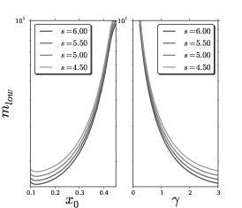
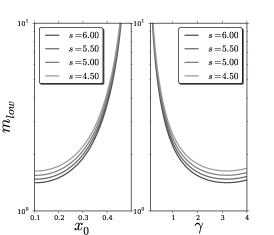
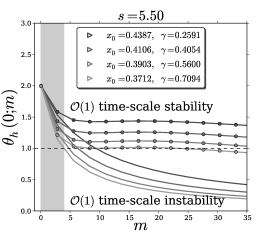
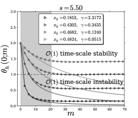
Fig. 11: Lower threshold $m_{\textrm{low}}$ versus $x_{0}$ and $\gamma$ for a steady-state stripe, as obtained by setting $\theta_{h}(0;m)=1$ in (4.23b). Plots are shown for several values of the aspect ratio parameter $s$. Under steady-state conditions, for a given $\gamma$, $x_{0}$ is determined from (4.38). In (a) the re-scaled parameter set one is given in Table 1, while in (b) the re-scaled parameter set two is given in Table 1. In the bottom row we plot $\theta_{h}(0;m)$ (solid curves), from (4.23b), and $\theta_{h0}(0;m)$ (dotted curves), from (4.28), when $s=5.5$ and for several pairs $(\gamma,x_{0})$ as obtained from the steady-state condition (4.38). All curves do eventually cross below the threshold $\theta_{h}(0;m)=1$, although for some curves this occurs outside the range of $m$ shown in the figure. In (c) the data set is from the re-scaled parameter set one in Table 1, while for (d) the data set is from the re-scaled parameter set two in Table 1.

We now illustrate our stability results for a steady-state stripe where $\gamma$ (and hence $k_{2}$ from (1.2b)) and $s$ are the primary bifurcation parameters. From Proposition 4.3 of [4] the steady-state stripe location $x_{0}$ for a given $\gamma>0$ is given by the unique root of

$$\frac{1}{6\beta\gamma D_{0}}\left(\frac{1}{2}-x_{0}\right)+\frac{\alpha^{\prime}(x_{0})}{\left[\alpha(x_{0})\right]^{2}}=0\,.$$ (4.38)

Since $\alpha^{\prime}(x_{0})<0$, it follows that $x_{0}$ satisfies $0<x_{0}<{1/2}$. Moreover, upon setting $\alpha(x_{0})=e^{-\nu x_{0}}$ in (4.38), we obtain that $x_{0}$ is a root of

$$6\beta D_{0}\nu\gamma={\mathcal{H}}(x_{0})\,,\qquad{\mathcal{H}}(x_{0})\equiv\left(\frac{1}{2}-x_{0}\right)e^{-\nu x_{0}}\,.$$ (4.39)

Since ${\mathcal{H}}^{\prime}(x_{0})<0$ on $0<x_{0}<{1/2}$, and $\gamma$ is inversely proportional to the auxin level $k_{2}$ at $x=0$, from (1.2b), it follows that the distance $x_{0}$ of the steady-state stripe from the left boundary increases as $k_{2}$ increases. This was shown numerically in Fig. 4.3 of [4].

Then, upon combining (4.39) with (4.31), we obtain that the lower edge $m_{0\textrm{low}}$ of the instability band for a steady-state stripe satisfies

$$G^{0}=\frac{1}{\nu}\left(\frac{1}{2}-x_{0}\right)\,.$$ (4.40)

Since ${dG^{0}/dx_{0}}>0$ on $0<x_{0}<{1/2}$ from Lemma 4.1, while the right-hand side of (4.40) is decreasing on $0<x_{0}<{1/2}$. it follows from the fact that ${dG^{0}/dm}<0$ (see Lemma 4.1), that $m_{0\textrm{low}}$ increases as $x_{0}$ increases. This leads to our key qualitative result that $m_{0\textrm{low}}$ increases as $\gamma$ decreases, or equivalently as $k_{2}$ increases. Thus, since the upper threshold $m_{0\textrm{up}}$ is independent of $k_{2}$, it follows that the width of the instability band in $m$ decreases when $k_{2}$ increases.

A second qualitative feature associated with (4.31) is with regards to the dependence of $m_{0\textrm{low}}$ on the aspect ratio parameter $s$. Since $G^{0}$ in (4.25) depends on $\mathchoice{{\hbox{$\displaystyle\sqrt{s\,}$}\lower 0.4pt\hbox{\vrule height=4.30554pt,depth=-3.44446pt}}}{{\hbox{$\textstyle\sqrt{s\,}$}\lower 0.4pt\hbox{\vrule height=4.30554pt,depth=-3.44446pt}}}{{\hbox{$\scriptstyle\sqrt{s\,}$}\lower 0.4pt\hbox{\vrule height=3.01389pt,depth=-2.41113pt}}}{{\hbox{$\scriptscriptstyle\sqrt{s\,}$}\lower 0.4pt\hbox{\vrule height=2.15277pt,depth=-1.72223pt}}}m$, it follows from (4.31) that the lower threshold $m_{0\textrm{low}}$ is proportional to ${1/\mathchoice{{\hbox{$\displaystyle\sqrt{s\,}$}\lower 0.4pt\hbox{\vrule height=4.30554pt,depth=-3.44446pt}}}{{\hbox{$\textstyle\sqrt{s\,}$}\lower 0.4pt\hbox{\vrule height=4.30554pt,depth=-3.44446pt}}}{{\hbox{$\scriptstyle\sqrt{s\,}$}\lower 0.4pt\hbox{\vrule height=3.01389pt,depth=-2.41113pt}}}{{\hbox{$\scriptscriptstyle\sqrt{s\,}$}\lower 0.4pt\hbox{\vrule height=2.15277pt,depth=-1.72223pt}}}}$, where $\mathchoice{{\hbox{$\displaystyle\sqrt{s\,}$}\lower 0.4pt\hbox{\vrule height=4.30554pt,depth=-3.44446pt}}}{{\hbox{$\textstyle\sqrt{s\,}$}\lower 0.4pt\hbox{\vrule height=4.30554pt,depth=-3.44446pt}}}{{\hbox{$\scriptstyle\sqrt{s\,}$}\lower 0.4pt\hbox{\vrule height=3.01389pt,depth=-2.41113pt}}}{{\hbox{$\scriptscriptstyle\sqrt{s\,}$}\lower 0.4pt\hbox{\vrule height=2.15277pt,depth=-1.72223pt}}}={L_{x}/L_{y}}$. Therefore, $m_{0\textrm{low}}$ is smaller for rectangular domains that are thinner in the transverse direction. In view of (4.27), $m_{0\textrm{up}}$ is also smaller for thin rectangular domains.

In Fig. 11–11 we plot $m_{\textrm{low}}$ versus $x_{0}$ and $\gamma$ for a steady-state stripe, as obtained by numerically determining the root of $\theta_{h}(0;m)=1$ from (4.23b). These plots are shown for several values of the aspect ratio parameter $s$. We remark that as $\gamma$ is varied, $x_{0}$ is calculated from the steady-state condition (4.38). The results are shown for the parameter set one (left figure) and two (right figure) in Table 1. In Fig. 11 and Fig. 11 we plot $\theta_{h}(0;m)$ from (4.23b) (solid curves) and $\theta_{h0}(0;m)$ from (4.28) (dotted curves) for the parameters set one and two given in Table 1, respectively. The results are shown for a fixed aspect ratio parameter $s=5.5$ for various pairs of $(x_{0},\gamma)$, related by the steady-state condition (4.38). We observe that there is better agreement for small modes in Fig. 11 rather than in Fig. 11. This results from the fact that parameter set two in Table 1 has a smaller value of $\varepsilon$, and is therefore closer to the asymptotic limit $\varepsilon\ll 1$ required by our stability analysis.

Finally, since the wavenumber $k$ of the unstable mode $m$ is given by $k=m/\pi$, the expected number of spots is given by the number of maxima of $\cos\left(k_{\textrm{max}}y\right)$ when

$$\frac{m_{\textrm{low}}}{\pi}<k_{\textrm{max}}<\mathchoice{{\hbox{$\displaystyle\sqrt{\frac{\upnu_{0}(c+r)}{\pi^{2}D_{1}}\,}$}\lower 0.4pt\hbox{\vrule height=14.31888pt,depth=-11.45515pt}}}{{\hbox{$\textstyle\sqrt{\frac{\upnu_{0}(c+r)}{\pi^{2}D_{1}}\,}$}\lower 0.4pt\hbox{\vrule height=10.0361pt,depth=-8.02892pt}}}{{\hbox{$\scriptstyle\sqrt{\frac{\upnu_{0}(c+r)}{\pi^{2}D_{1}}\,}$}\lower 0.4pt\hbox{\vrule height=7.40414pt,depth=-5.92334pt}}}{{\hbox{$\scriptscriptstyle\sqrt{\frac{\upnu_{0}(c+r)}{\pi^{2}D_{1}}\,}$}\lower 0.4pt\hbox{\vrule height=7.40414pt,depth=-5.92334pt}}}L_{y}\,,$$

where $k_{\textrm{max}}$ corresponds to the integer nearest the location of the maximum of the dispersion relation.

To determine the dispersion relation and the maximum growth rate, we must numerically compute the spectrum of the NLEP (4.23) within the instability band. Our computations are done for the parameter set three given in Table 1, which is a further modification of the set one. To do so, we use a standard three point uniform finite differences method to discretize (4.23a) to obtain a nonlinear eigenvalue problem, and then apply a backwards iterative process on $m$. In order to perform this computation, $m$ is treated as a continuous variable. The results are shown in Fig. 12 in the plot of $\Re(\lambda)$ versus $k={m/\pi}$. In Fig. 12 we plot the dispersion relation for a fixed $x_{0}$ but for several different aspect ratio parameters. From this figure we observe that the most unstable mode increases as $s$ decreases, or equivalently as the transverse width $L_{y}$ of the domain increases. As a consequence, we predict that as the domain width in the transverse direction increases, a larger number of spots can emerge after a breakup instability.

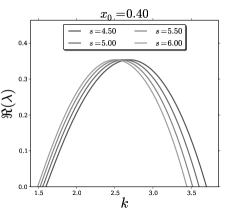
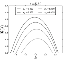
Fig. 12: Dispersion relation $\Re(\lambda)$ versus $k$ for a steady-state interior localised stripe. In (a) we fix $x_{0}=0.4$ (and hence $\gamma$ by (4.38)) and plot the dispersion relation for several aspect ratio parameters $s$. In (b) we fix $s=5.5$ and plot the dispersion relation for several steady-state pairs of $(x_{0},\gamma)$. The re-scaled parameter set three, given in Table 1, was used. The nearest integer value of $k$ to the location of the maximum of these curves is the theoretically predicted number of spots to form from the break up of the stripe.

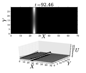
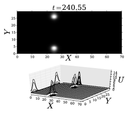
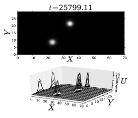
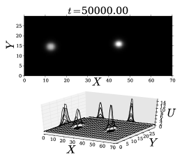
Fig. 13: Breakup instability and secondary $\mathcal{O}(1)$ time-scale instabilities of an interior localised stripe for $U$. (a) The localised stripe initially breaks into two spots; (b) once formed, the spots migrate from the boundary towards each other along the $x$-location line, and (c) rotate until they get aligned with the longitudinal direction. (d) Finally, they get pinned far from each other. Original parameter set three as given in Table 1 with $k_{2}=0.5$, which corresponds to a stripe location at $x_{0}=24.5$.

On the other hand, in Fig. 12, by fixing the aspect ratio $s$, we show that as $x_{0}$ decreases, or equivalently as $\gamma$ increases (or $k_{2}$ decreases), the growth rate for an instability increases rather substantially, with only a slight shift in the location of the most unstable mode. Therefore, even though the steady-state stripe location only slightly influences the number of spots that are predicted from the break up of the stripe, larger values of $\gamma$, or equivalently smaller values of $k_{2}$, will promote a wider band of unstable modes and a rather large increase in the growth rate of the most unstable mode. Therefore, this suggests that an interior stripe is more sensitive to a transverse instability if it is located closer to the left-hand boundary, where the influence of the auxin gradient is the strongest.

The dispersion relation for an interior stripe with $s=5.5$ and $x_{0}=0.35$ is the top curve in Fig. 12. It predicts that the stripe will break up into either two or three spots. To confirm this theoretical prediction, we take the stripe as the initial condition and perform a direct numerical simulation of the full PDE system (4.7) for the parameter set three in Table 1. The results are shown in Fig. 13, where we observe from Fig. 13 and Fig. 13 that the stripe initially breaks into two distinct localised spots. The spatial dynamics of these two newly-created spots is controlled by the auxin gradient. They initially move closer to each other along a vertical line, and then rotate slowly in a clockwise direction to eventually become aligned with the horizontal direction associated with the auxin gradient $\alpha(x)$ (see Fig. 13). Finally, in Fig. 13 we show a stable equilibrium configuration of two spots lying along the centre line of the transverse direction. An open problem, beyond the scope of this paper, is to characterise the dynamics and instabilities of spot patterns in the presence of the auxin gradient.

4.2 A Boundary Stripe

The bifurcation diagram depicted in Fig. 4 shows all branches to be linearly unstable under transverse perturbations, except for a narrow window on the boundary stripe branch. In this section we will derive and analyse the NLEP associated with a boundary stripe centred at $x=0$. We remark that the stability of a boundary stripe was not investigated in the prior studies of [7] and [14]. Although we give only a formal derivation of the NLEP, we will obtain rigorous results for the spectrum of the NLEP.

A steady-state boundary spike $(u_{s},v_{s})$ centred at $x=0$ was constructed asymptotically in the limit $\varepsilon\to 0$ in Proposition 4.4 of [4], with the result

$$v_{s}\sim v_{b}^{0}+\left(-\frac{x^{2}}{2D_{0}}+\frac{x}{D_{0}}\right)\,,\qquad u_{s}\sim\frac{1}{\alpha(0)v_{b}^{0}}w\left({x/\varepsilon}\right)\,,\qquad v_{b}^{0}=\frac{3\beta\gamma}{\alpha(0)}\,,$$ (4.41)

where $w(\xi)=({3/2})\,\textnormal{sech}^{2}({\xi/2})$ is the even homoclinic solution of $w^{\prime\prime}-w+w^{2}=0$. Upon substituting (4.41) into (4.7), we obtain the eigenvalue problem (4.9) characterizing transverse instabilities on an ${\mathcal{O}}(1)$ time-scale.

We then look for a localised eigenfunction for $\varphi(x)$ in the form

$$\Phi_{b}(\xi)=\varphi(\varepsilon\xi)\,,\qquad\xi\equiv\varepsilon^{-1}x\,.$$ (4.42)

From (4.41) we calculate $2u_{s}v_{s}\alpha\sim 2w$ and $\alpha u_{s}^{2}\sim{\alpha(0)w^{2}/\left[\alpha(0)v^{0}\right]^{2}}$ for $x$ near $0$. In this way, we obtain from (4.9a) that $\Phi_{b}(\xi)\sim\Phi_{b0}(\xi)+o(1)$, where $\Phi_{b0}$ satisfies

$${\mathcal{L}}_{0}\Phi_{b0}+\frac{w^{2}}{\alpha(0)\left[v_{b}^{0}\right]^{2}}\psi(0)=\left(\lambda+s\varepsilon^{2}m^{2}\right)\Phi_{b0}\,,\quad\xi\geq 0\,;\qquad\Phi_{b0\xi}(0)=0\,,\quad\Phi_{b0}\to 0\,\quad\mbox{as}\quad\xi\to\infty\,.$$ (4.43)

Here $\mathcal{L}_{0}\Phi_{b0}\equiv\Phi_{b0\xi\xi}-\Phi_{b0}+2w\Phi_{b0}$.

Next, we must calculate $\psi(0)$ in (4.43) from (4.9b). To do so, we use (4.41) and (4.42) for $u_{s}$, $v_{s}$, and $\varphi$, and we integrate (4.9b) over $0<x<\delta$, where $\delta$ is an intermediate scale between the inner and outer regions satisfying ${\mathcal{O}}(\varepsilon)\ll\delta\ll{\mathcal{O}}(1)$. In this way, we obtain

$$D_{0}\psi_{x}|_{0}^{\delta}+{\mathcal{O}}(\delta)-\frac{\tau\gamma\psi(0)}{\alpha(0)\left[v_{b}^{0}\right]^{2}}\int_{0}^{\delta/\varepsilon}w^{2}\,d\xi+{\mathcal{O}}(\varepsilon\delta)=2\tau\gamma\int_{0}^{\delta/\varepsilon}\left(w\Phi_{b0}-\kappa\Phi_{b0}\right)\,d\xi+{\mathcal{O}}(\varepsilon\delta\tau\lambda)\,,$$

where $\kappa\equiv{\left(1-{\beta/\tau}\right)/2}$. Since $\delta\gg{\mathcal{O}}(\varepsilon)$ and $\int_{0}^{\infty}w^{2}\,d\xi=3$, we obtain in the limit $\delta\to 0$ with ${\delta/\varepsilon}\gg 1$ that

$$D_{0}\psi_{x}(0^{+})\equiv\frac{3\tau\gamma\psi(0)}{\alpha(0)\left[v_{b}^{0}\right]^{2}}+2\tau\gamma\int_{0}^{\infty}\left(w\Phi_{b0}-\kappa\Phi_{b0}\right)\,d\xi\,.$$ (4.44)

In this way, we obtain from (4.9b) and (4.44) that the leading-order outer solution $\psi_{0}$ for $\psi$ satisfies

$$\psi_{0xx}-sm^{2}\psi_{0}=0\,,\qquad 0<x\leq 1\,;\qquad\psi_{0x}(1)=0\,;\qquad D_{0}\psi_{0x}(0^{+})=\frac{a_{b}}{\gamma}\psi_{0}(0)+\gamma b_{b}\,,$$ (4.45)

where, upon using (4.41) for $v_{b}^{0}$, we have defined $a_{b}$ and $b_{b}$ by

$$a_{b}\equiv\frac{\tau\alpha(0)}{3\beta^{2}}\,,\qquad b_{b}\equiv 2\tau\int_{0}^{\infty}\left(w\Phi_{b0}-\kappa\Phi_{b0}\right)\,d\xi\,,\qquad\kappa\equiv\frac{1}{2}\left(1-\frac{\beta}{\tau}\right)\,.$$ (4.46)

The solution to the ODE in (4.45) with $\psi_{0x}(1)=0$ is $\psi_{0}(x)=A\cosh\left[\mathchoice{{\hbox{$\displaystyle\sqrt{s\,}$}\lower 0.4pt\hbox{\vrule height=4.30554pt,depth=-3.44446pt}}}{{\hbox{$\textstyle\sqrt{s\,}$}\lower 0.4pt\hbox{\vrule height=4.30554pt,depth=-3.44446pt}}}{{\hbox{$\scriptstyle\sqrt{s\,}$}\lower 0.4pt\hbox{\vrule height=3.01389pt,depth=-2.41113pt}}}{{\hbox{$\scriptscriptstyle\sqrt{s\,}$}\lower 0.4pt\hbox{\vrule height=2.15277pt,depth=-1.72223pt}}}m(x-1)\right]$. The constant $A$ is found by satisfying the condition in (4.45) at $x=0$, which then determines $\psi_{0}(0)$ as

$$\psi_{0}(0)=-\frac{\gamma^{2}b_{b}}{a_{b}+D_{0}\gamma\mathchoice{{\hbox{$\displaystyle\sqrt{s\,}$}\lower 0.4pt\hbox{\vrule height=4.30554pt,depth=-3.44446pt}}}{{\hbox{$\textstyle\sqrt{s\,}$}\lower 0.4pt\hbox{\vrule height=4.30554pt,depth=-3.44446pt}}}{{\hbox{$\scriptstyle\sqrt{s\,}$}\lower 0.4pt\hbox{\vrule height=3.01389pt,depth=-2.41113pt}}}{{\hbox{$\scriptscriptstyle\sqrt{s\,}$}\lower 0.4pt\hbox{\vrule height=2.15277pt,depth=-1.72223pt}}}m\tanh\left(\mathchoice{{\hbox{$\displaystyle\sqrt{s\,}$}\lower 0.4pt\hbox{\vrule height=4.30554pt,depth=-3.44446pt}}}{{\hbox{$\textstyle\sqrt{s\,}$}\lower 0.4pt\hbox{\vrule height=4.30554pt,depth=-3.44446pt}}}{{\hbox{$\scriptstyle\sqrt{s\,}$}\lower 0.4pt\hbox{\vrule height=3.01389pt,depth=-2.41113pt}}}{{\hbox{$\scriptscriptstyle\sqrt{s\,}$}\lower 0.4pt\hbox{\vrule height=2.15277pt,depth=-1.72223pt}}}m\right)}\,.$$

Upon substituting $\psi_{0}(0)$ into (4.43), and by using (4.46) for $a_{b}$ and $b_{b}$, we obtain after some re-arrangement that

$${\mathcal{L}}_{0}\Phi_{b0}-\frac{\mu_{b}}{3}w^{2}\left(I_{1}-\kappa I_{2}\right)=\left(\lambda+\varepsilon^{2}sm^{2}\right)\Phi_{b0}\,,\quad\xi\geq 0\,;\qquad\Phi_{b0\xi}(0)=0\,,\quad\Phi_{b0}\to 0\,\quad\mbox{as}\quad\xi\to\infty\,.$$ (4.47)

In (4.47), we have defined $\mu_{b}$, $I_{1}$, and $I_{2}$, by

$$\mu_{b}\equiv\frac{2}{1+\chi_{b}\mathchoice{{\hbox{$\displaystyle\sqrt{s\,}$}\lower 0.4pt\hbox{\vrule height=4.30554pt,depth=-3.44446pt}}}{{\hbox{$\textstyle\sqrt{s\,}$}\lower 0.4pt\hbox{\vrule height=4.30554pt,depth=-3.44446pt}}}{{\hbox{$\scriptstyle\sqrt{s\,}$}\lower 0.4pt\hbox{\vrule height=3.01389pt,depth=-2.41113pt}}}{{\hbox{$\scriptscriptstyle\sqrt{s\,}$}\lower 0.4pt\hbox{\vrule height=2.15277pt,depth=-1.72223pt}}}m\tanh\left(\mathchoice{{\hbox{$\displaystyle\sqrt{s\,}$}\lower 0.4pt\hbox{\vrule height=4.30554pt,depth=-3.44446pt}}}{{\hbox{$\textstyle\sqrt{s\,}$}\lower 0.4pt\hbox{\vrule height=4.30554pt,depth=-3.44446pt}}}{{\hbox{$\scriptstyle\sqrt{s\,}$}\lower 0.4pt\hbox{\vrule height=3.01389pt,depth=-2.41113pt}}}{{\hbox{$\scriptscriptstyle\sqrt{s\,}$}\lower 0.4pt\hbox{\vrule height=2.15277pt,depth=-1.72223pt}}}m\right)}\,,\qquad\chi_{b}\equiv\frac{3D_{0}\beta^{2}\gamma}{\tau\alpha(0)}\,,\qquad I_{1}\equiv\int_{0}^{\infty}w\Phi_{b0}\,d\xi\,,\qquad I_{2}\equiv\int_{0}^{\infty}\Phi_{b0}\,d\xi\,.$$ (4.48)

Next, we integrate (4.47) over $\xi\geq 0$ and use $\int_{0}^{\infty}w^{2}\,d\xi=3$ to obtain the relation (4.22) between $I_{1}$ and $I_{2}$. Finally, the NLEP for the boundary stripe is obtained by eliminating $I_{2}$ in (4.47). We summarise our result for the NLEP as follows:

Proposition 4.4.

The stability on an ${\mathcal{O}}(1)$ time-scale of a steady-state boundary stripe solution of (4.7) is determined by the spectrum of the NLEP

$${\mathcal{L}}_{0}\Phi_{b0}-\theta_{b}(\lambda;m)\,w^{2}\>\frac{\int_{0}^{\infty}w\Phi_{b0}\>d\xi}{\int_{0}^{\infty}w^{2}\,d\xi}=\left(\lambda+s\varepsilon^{2}m^{2}\right)\Phi_{0}\,,\qquad 0\leq\xi<\infty\,;\qquad\Phi_{b0}\to 0\quad\mbox{as}\quad|\xi|\to\infty\,,$$ (4.49a)

with $$\Phi_{b0\xi}(0)=0 \mathcal{L}_{0}\Phi_{b0}\equiv\Phi_{b0\xi\xi}-\Phi_{b0}+2w\Phi_{b0} \theta_{b}(\lambda;m)$$ and . Here is given by

$$\theta_{b}(\lambda;m)\equiv\mu_{b}\left(\frac{\lambda+1+s\varepsilon^{2}m^{2}-2\kappa}{\lambda+1+s\varepsilon^{2}m^{2}-\mu_{b}\kappa}\right)\,,\qquad\kappa\equiv\frac{1}{2}\left(1-\frac{\beta}{\tau}\right)\,,$$ (4.49b)

$$\mu_{b}\equiv\frac{2}{1+\chi_{b}\mathchoice{{\hbox{$\displaystyle\sqrt{s\,}$}\lower 0.4pt\hbox{\vrule height=4.30554pt,depth=-3.44446pt}}}{{\hbox{$\textstyle\sqrt{s\,}$}\lower 0.4pt\hbox{\vrule height=4.30554pt,depth=-3.44446pt}}}{{\hbox{$\scriptstyle\sqrt{s\,}$}\lower 0.4pt\hbox{\vrule height=3.01389pt,depth=-2.41113pt}}}{{\hbox{$\scriptscriptstyle\sqrt{s\,}$}\lower 0.4pt\hbox{\vrule height=2.15277pt,depth=-1.72223pt}}}m\tanh\left(\mathchoice{{\hbox{$\displaystyle\sqrt{s\,}$}\lower 0.4pt\hbox{\vrule height=4.30554pt,depth=-3.44446pt}}}{{\hbox{$\textstyle\sqrt{s\,}$}\lower 0.4pt\hbox{\vrule height=4.30554pt,depth=-3.44446pt}}}{{\hbox{$\scriptstyle\sqrt{s\,}$}\lower 0.4pt\hbox{\vrule height=3.01389pt,depth=-2.41113pt}}}{{\hbox{$\scriptscriptstyle\sqrt{s\,}$}\lower 0.4pt\hbox{\vrule height=2.15277pt,depth=-1.72223pt}}}m\right)}\,,\qquad\chi_{b}\equiv\frac{3D_{0}\beta^{2}\gamma}{\tau\alpha(0)}\,.$$ (4.49c)

We remark that to incorporate the homogeneous Neumann boundary condition at $\xi=0$, we can simply extend $\Phi_{b0}$ to be an even function of $\xi$ and replace the range $0<\xi<\infty$ of integration in the two integrals in (4.49a) to be $-\infty<\xi<\infty$. In this way, we can use the NLEP stability theory of §4.1 for an interior stripe.

We first observe that $\mu_{b}=\mu_{b}(m)$ satisfies $\mu_{b}(0)=2$, $\mu_{b}={\mathcal{O}}({1/m})$ for $m\gg 1$, and ${d\mu_{b}/dm}<0$ for $m>0$. As a consequence of this behavior for $\mu_{b}$, we obtain, as for the case of the interior stripe, the following proposition:

Proposition 4.5.

The NLEP in (4.49) has a unique unstable eigenvalue when $m$ lies within an instability band $0<m_{\textrm{\em low}}<m<m_{\textrm{\em up}}$, with $m_{\textrm{\em low}}={\mathcal{O}}(1)$ and $m_{\textrm{\em up}}={\mathcal{O}}\left(\varepsilon^{-1}\right)$.

Since the proof of Proposition 4.5 parallels that in §4.1, we only outline the derivation. However, we remark that since $\mu_{b}(0)=2$, we have $\theta_{b}(\lambda;0)=2$ for all $\lambda$. Since $\theta_{b}(\lambda;0)=2>1$, we conclude from Lemma A and Theorem 1.3 of [30] that $\Re(\lambda)<0$, and so a 1D boundary spike is stable on an ${\mathcal{O}}(1)$ time-scale for any choice of the parameters $\beta$, $\tau$, and $\gamma$.

Next, since $\mu_{b}={\mathcal{O}}({1/m})$ for $m\gg 1$, we conclude from (4.49b) that $\theta_{b}={\mathcal{O}}(\varepsilon)$ when $m={\mathcal{O}}(\varepsilon^{-1})$. As such, we conclude as in §4.1 (see (4.26)–(4.27)) that, on the regime $m={\mathcal{O}}(\varepsilon^{-1})$, the boundary stripe is stable when $m>m_{\textrm{up}}$ and is unstable when $m<m_{\textrm{up}}$, where $m_{\textrm{up}}$ is defined in (4.27). To determine the lower edge of the instability band, which occurs on the regime $\varepsilon m\ll 1$, we set $\theta_{b}(0;m)=1$. Upon using (4.49b) where $\varepsilon m\ll 1$, we readily obtain that $m_{\textrm{low}}\sim{z_{\textrm{low}}/\mathchoice{{\hbox{$\displaystyle\sqrt{s\,}$}\lower 0.4pt\hbox{\vrule height=4.30554pt,depth=-3.44446pt}}}{{\hbox{$\textstyle\sqrt{s\,}$}\lower 0.4pt\hbox{\vrule height=4.30554pt,depth=-3.44446pt}}}{{\hbox{$\scriptstyle\sqrt{s\,}$}\lower 0.4pt\hbox{\vrule height=3.01389pt,depth=-2.41113pt}}}{{\hbox{$\scriptscriptstyle\sqrt{s\,}$}\lower 0.4pt\hbox{\vrule height=2.15277pt,depth=-1.72223pt}}}}$, where $z=z_{\textrm{low}}$ is the unique root of

$$z\tanh(z)=\frac{1-2\kappa}{\chi_{b}}=\frac{\beta}{\tau\chi_{b}}\,,\qquad\chi_{b}\equiv\frac{3D_{0}\beta^{2}\gamma}{\tau\alpha(0)}\,,$$ (4.50)

where $\alpha(0)=1$. The unstable discrete eigenvalues of the NLEP (4.49) are characterized as follows:

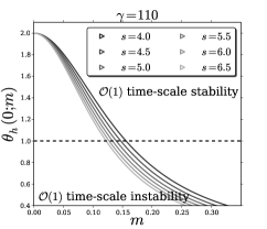
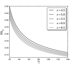
Fig. 14: (a) Plot of $\theta_{b}(0;m)$ versus $m$ as obtained from (4.49b). (b) The lower edge $m_{\textrm{low}}$ of the instability band versus $\gamma$ for several values of the aspect ratio parameter $s$. From (4.50), $m_{\textrm{low}}$ is proportional to ${1/\mathchoice{{\hbox{$\displaystyle\sqrt{s\,}$}\lower 0.4pt\hbox{\vrule height=4.30554pt,depth=-3.44446pt}}}{{\hbox{$\textstyle\sqrt{s\,}$}\lower 0.4pt\hbox{\vrule height=4.30554pt,depth=-3.44446pt}}}{{\hbox{$\scriptstyle\sqrt{s\,}$}\lower 0.4pt\hbox{\vrule height=3.01389pt,depth=-2.41113pt}}}{{\hbox{$\scriptscriptstyle\sqrt{s\,}$}\lower 0.4pt\hbox{\vrule height=2.15277pt,depth=-1.72223pt}}}}$ and $m_{\textrm{low}}$ decreases as $\gamma$ increases. Recall from (1.2b) that $\gamma$ is inversely proportional to $k_{2}$, representing the non-dimensional auxin concentration at $x=0$. Re-scaled parameter set three as given in Table 1.

Proposition 4.6.

Let $\varepsilon m\ll 1$, and let $N$ denote the number of eigenvalues of the NLEP of (4.49) in $\Re(\lambda)>0$. Then, for $m$ on the range $m\ll{\mathcal{O}}(\varepsilon^{-1})$ as $\varepsilon\to 0^{+}$, we have

• (I): $\quad N=1$ if $m>m_{0\textrm{\em low}}$. The unique real unstable eigenvalue $\lambda_{0}$ satisfies $0<\lambda_{0}<\upnu_{0}$. Here, for $\varepsilon\to 0$, $m_{0\textrm{\em low}}={z_{\textrm{\em low}}/\mathchoice{{\hbox{$\displaystyle\sqrt{s\,}$}\lower 0.4pt\hbox{\vrule height=4.30554pt,depth=-3.44446pt}}}{{\hbox{$\textstyle\sqrt{s\,}$}\lower 0.4pt\hbox{\vrule height=4.30554pt,depth=-3.44446pt}}}{{\hbox{$\scriptstyle\sqrt{s\,}$}\lower 0.4pt\hbox{\vrule height=3.01389pt,depth=-2.41113pt}}}{{\hbox{$\scriptscriptstyle\sqrt{s\,}$}\lower 0.4pt\hbox{\vrule height=2.15277pt,depth=-1.72223pt}}}}$ and $z_{\textrm{\em low}}$ is the unique root of (4.50).

• (II): $\quad N=0$ if $0<m<m_{0\textrm{\em low}}$.

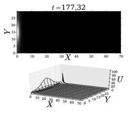
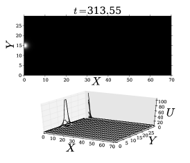
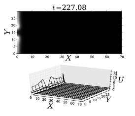
Fig. 15: Breakup instability for $U$ of a boundary stripe for two different values of $k_{2}$. Initial snapping as (a) $k_{2}=0.0013$ and (c) $k_{2}=0.4$; from there (b) one and (d) four spots are formed at the boundary. The original parameter set three, given in Table 1, is used. The parameter values $k_{2}=0.0013$ and $k_{2}=0.4$ correspond to $\gamma=115$ and $\gamma=0.375$ respectively in terms of the re-scaled variables.

The proof of this result is exactly the same as for the interior stripe case, as given in Proposition 4.3, and is omitted.

In Fig. 14 we plot $\theta_{b}(0;m)$ versus $m$ for several values of the aspect ratio parameter $s$. The other data values are set as in Table 1 for the parameter set three. As shown in the proof of Proposition 4.3, the NLEP (4.49) has an unstable eigenvalue when $\theta_{b}(0;m)<1$. In Fig. 14 we plot the lower edge $m_{\textrm{low}}$ of the instability band versus $\gamma$ for several values of $s$, as obtained from numerically determining the root of $\theta_{b}(0;m)=1$ from (4.49b). For $\varepsilon\ll 1$, we have that $m_{\textrm{low}}\sim m_{0\textrm{low}}\equiv{z_{\textrm{low}}/\mathchoice{{\hbox{$\displaystyle\sqrt{s\,}$}\lower 0.4pt\hbox{\vrule height=4.30554pt,depth=-3.44446pt}}}{{\hbox{$\textstyle\sqrt{s\,}$}\lower 0.4pt\hbox{\vrule height=4.30554pt,depth=-3.44446pt}}}{{\hbox{$\scriptstyle\sqrt{s\,}$}\lower 0.4pt\hbox{\vrule height=3.01389pt,depth=-2.41113pt}}}{{\hbox{$\scriptscriptstyle\sqrt{s\,}$}\lower 0.4pt\hbox{\vrule height=2.15277pt,depth=-1.72223pt}}}}$, where $z_{\textrm{low}}$ is the unique root of (4.50). From (4.50), we conclude that $m_{0\textrm{low}}$ is proportional to ${1/\mathchoice{{\hbox{$\displaystyle\sqrt{s\,}$}\lower 0.4pt\hbox{\vrule height=4.30554pt,depth=-3.44446pt}}}{{\hbox{$\textstyle\sqrt{s\,}$}\lower 0.4pt\hbox{\vrule height=4.30554pt,depth=-3.44446pt}}}{{\hbox{$\scriptstyle\sqrt{s\,}$}\lower 0.4pt\hbox{\vrule height=3.01389pt,depth=-2.41113pt}}}{{\hbox{$\scriptscriptstyle\sqrt{s\,}$}\lower 0.4pt\hbox{\vrule height=2.15277pt,depth=-1.72223pt}}}}$ and that $m_{0\textrm{low}}$ decreases as $\gamma$ increases. Since $\gamma$ is inversely proportional to the non-dimensional auxin concentration $k_{2}$ at $x=0$ (see (1.2b)), it follows that $m_{\textrm{low}}$ is larger for larger values of $k_{2}$ when $\varepsilon\ll 1$. Recall that the upper edge $m_{\textrm{up}}$ of the instability band is independent of $k_{2}$ and only depends on $s$ and $\varepsilon$. As such, we expect that the location $m_{\textrm{max}}$ of the maximum growth rate is larger for larger $k_{2}$, suggesting that as $k_{2}$ is increased the boundary stripe will break up into an increasing number of spots.

To test this prediction, we solve the full RD system (1.1) numerically with a boundary stripe as the initial condition. Two simulations are performed; one for a small value of $k_{2}=0.0013$, corresponding to $\gamma=115$, and one with the larger value $k_{2}=0.4$, for which $\gamma=0.375$. The other parameter values are fixed as in Table 1 for the parameter set three. For $k_{2}=0.0013$, in Fig. 15 we show that the boundary stripe breaks up into one spot, which is eventually formed at the midpoint of the transversal length (see Fig. 15). In contrast, for the larger value $k_{2}=0.4$, in Fig. 15 we show that the boundary stripe initially begins to break in two, ultimately leading to four spots along the boundary, as shown in Fig. 15. These results confirm the theoretical prediction that a boundary stripe will break up into a larger number of spots as $k_{2}$ is increased.

5 Conclusions

This paper has sought to make more realistic the analysis began in [4] of a generalised Schnakenberg system with a spatial gradient of the active nonlinear term. The model seeks to explain the auxin-mediated action of ROPs in an Arabidopsis root hair cell leading to the creation of a unique isolated patch of active ROP from which hair formation is initiated. The choice of a rectangular 2D domain and homogeneous auxin concentration in the $y$-direction in this work was motivated by a compromise between more biological realism and mathematical tractability. Realistically, the reactions we model are thought to take place in the cytosol of the plant cell, which in a thin domain occupying the space between the cell wall and the cell vacuole, the high-pressure void within plant cells that maintains turgor pressure. Modelling the portion of this space that abuts the root epidermis, we have in reality a thin slice formed out of a fixed circumferential arc of the space between two concentric cylinders. We have simplified this domain in two ways. First, we have ignored diffusion in the radial direction, although in effect this is captured by the much larger diffusion constant of the inactive ROPs that are free to move in all radial position compared with the active from, that is bound to the outer wall. Second, we have ignored curvature, as we do not believe this is likely to affect diffusion significantly and can be approximated by small adjustments to diffusion constants.

The other simplification we have chosen is to assume no $y$-dependence on the auxin gradient. In a sense this is the simplest possible assumption given that evidence currently in the literature so-far only supports a gradient in the $x$-direction [11], with no information on $y$-dependence. A key test then is whether in the absence of any $y$-gradient, a spot-like rather than a stripe-like patch will occur.

Broadly speaking, our analysis and computations support the conclusions reached in 1D. For low $k_{2}$-values (low overall auxin concentration or short cells) there is a patch of active ROP that is confined to the basal end of the cell. As $k_{2}$ is increased there is a bifurcation into states which have increasing numbers of spots, which correspond to either wild type (where there would be a unique interior spot) and various multiple hair mutant types in which auxin is increased to much higher levels. Owing to the presence of fold bifurcations, there is an overlap between the parameter intervals in which the different states exist, which suggests hysteretic transitions upon increase and decrease of the bifurcation parameter. In [4] this property was argued to be crucial and to imply biological robustness; a cell that is in the process of forming a single hair would not reverse this process or start growing an extra one if the auxin concentration were to suddenly change. Moreover, owing to the auxin gradient $k_{2}\alpha(x)$, spot-like patches first form where the auxin concentration is highest, that is towards the basal end of the cell, as observed in wild type.

Another encouraging finding has been that we have found the instability of stripes into spot-like states occurs on an $\mathcal{O}(1)$ time-scale. This means that once the boundary patch of active ROP switches into the cell interior, it quickly, on an $\mathcal{O}(1)$ time-scale, breaks up into spots. Note that there can therefore be no multi-stripe interior states either. This is an important implication as the transition into a spot-like state can be interpreted as a minimising energy (maximising entropy) thermodynamical process. That is, in order to maintain a sufficient supply of active ROP to induce localised cell wall softening, the aggregation process follows the least energy cost.

One weakness of our results though is that the analysis of the $\mathcal{O}(1)$ times-cale instability is only really tractable due to the Neumann boundary conditions in $y$ and homogeneity of the auxin in the $y$-direction. One biologically unrealistic consequence of this simplification is that there is no preference for spot-like patches to form on the lateral mid-line; there is an equal chance that half-spots can form at the transverse edge of the domain. In reality, softening cell wall patches always occur along the mid-line of the cell. It seems then that a more complete mathematical model of the root hair patterning process would require some non-trivial $y$-dependence in order to pin spots transversly. This could easily be accounted for by the nature of the transport of auxin into neighbouring non-root-hair cells as suggested by [11] (see also [10] for a modelling approach). The analytic approach developed here would no longer be applicable in this case. An investigation of these effects is left to future work. This could be modelled by either allowing an auxin gradient in both directions or by having traverse boundary conditions of Robin type. Such an analysis is beyond the scope of this paper, and is left to future work.

Another connection that is left for future work is the understanding of the multi-spot solutions in terms of the theory of so-called homoclinic snaking [5, 32] in which multiple localised patterns coexist with stable periodic and homogeneous background states. Recently [3] we showed that the spatially homogeneous version of the system investigated here in 1D satisfies all the ingredients of that theory, which explains the presence of localised patterns of arbitrary wide spatial extent (provided the domain is long enough). The inclusion of a gradient $\alpha(x)$ multiplying the main bifurcation parameter $k_{2}$, ensures that all these localised branches do not coexist for asymptotically the same parameter intervals, but at parameter intervals that drift as the parameter value is changed, so called “slanted snaking” [6]. This slant occurs, in effect, because the local value of the parameter $k_{2}\alpha(x)$ decreases as the centre of the localised pattern shifts to the right. An analysis of the bifurcation diagram of localised 2D patterns in this system using such methods is left for future work, but we note the subtleties that can occur in rectangular domains [2].

Acknowledgements. The research of V. F. B–M. for this work was supported by a CONACyT grant from the Mexican government and additional financial support from the UK EPSRC. M. J. W. was supported by NSERC grant 81541.

References

• [1] J. L. Aragón, R. A. Barrio, T. E. Woolley, R. E. Baker, and P. K. Maini, Nonlinear effects on Turing patterns: Time oscillations and chaos, Phys. Rev. E, 86 (2012), p. 026201.
• [2] D. Avitabile, D. Lloyd, J. Burke, E. Knobloch, and B. Sandstede, To snake or not to snake in the planar swift–hohenberg equation, SIAM Journal of Applied Dynamical Systems, 9 (2010), pp. 704–733.
• [3] V. Brena–Medina and A. R. Champneys, Subcritical Turing bifurcation and the morphogenesis of localized structures, Phys. Rev. E, 90 (2014), p. 032923.
• [4] V. Brena–Medina, A. R. Champneys, C. Grierson, and M. J. Ward, Mathematical modelling of plant root hair initiation; dynamics of localized patches, SIAM J. Applied Dynamical Systems, 13 (2014), pp. 210–248.
• [5] J. Burke and E. Knobloch, Snakes and ladders: Localized states in the Swift–Hohenberg equation, Physics Letters A, 360 (2006), pp. 681–688.
• [6] J.H.P. Dawes, Localized pattern formation with a large-scale mode: Slanted snaking, SIAM J. Applied Dynamical Systems, 7 (2008), pp. 186–206.
• [7] A. Doelman and H. van der Ploeg, Homoclinic stripe patterns, SIAM Journal on Applied Dynamical Systems, 1 (2002), pp. 65–104.
• [8] A. Gierer and H. Meinhardt, A theory of biological pattern formation, Biological Cybernetics, 12 (1972), pp. 30–39.
• [9] M. Golubitsky and D. Schaeffer, Singularities and Groups in Bifurcation Theory, vol. 1, New York: Springer–Verlag, 1985.
• [10] V.A. Grieneisen, A.F. Maree, P. Hogeweg, and B. Scheres, Auxin transport is sufficient to generate a maximum and gradient guiding root growth, Nature, 449 (2007), pp. 1008–1013.
• [11] A.R. Jones, E.M. Kramer, K. Knox, R. Swarup, M.J. Bennett, C.M. Lazary, H.M. Ottoline Leyser, and C.S. Grierson, Auxin transport through non-hair cells sustains root-hair development, Nat. Cell. Biol., 11 (2009), pp. 78–84.
• [12] M. A. Jones, J–J. Shen, Y. Fu, H. Li, Z. Yang, and C. Grierson, The Arabidopsis Rop2 GTPase is a positive regulator of both root hair initiation and tip growth, The Plant Cell, 14 (2002), pp. 763–776.
• [13] A. J. Koch and H. Meinhardt, Biological pattern formation: from basic mechanisms to complex structures, Rev. Mod. Phys., 66 (1994), pp. 1481–1507.
• [14] T. Kolokolnikov, W. Sun, M. J. Ward, and J. Wei, The stability of a stripe for the Gierer–Meinhardt model and the effect of saturation, SIAM J. Applied Dynamical Systems, 5 (2006), pp. 313–363.
• [15] T. Kolokolnikov, M.J. Ward, and J. Wei, Spot self-replication and dynamics for the Schnakenberg model in a two-dimensional domain, J. Nonlinear Sci., 19 (2009), pp. 1–56.
• [16] T. Kolokolnikov and M. J. Ward, Reduced wave Green’s functions and their effect on the dynamics of a spike for the Gierer–Meinhardt model, Europ. J. Appl. Math., 14 (2003), pp. 513–545.
• [17] T. Kolokolnikov, M. J. Ward, and J. Wei, Zigzag and breakup instabilties of stripes and rings in the two-dimensional Gray–Scott model, Studies in Appl. Math., 16 (2006), pp. 35–95.
• [18] E. M. Kramer, Auxin-regulated cell polarity: an inside job?, Cell, (2009), pp. 1360–1385.
• [19] C. S. Lin, W. M. Ni, and I. Takagi, Large amplitude stationary solutions to a chemotaxis system, J. Diff. Eq., 72 (1988), pp. 1–27.
• [20] H. Meinhardt, The algorithmic beauty of sea shells, Springer–Verlag New York, Inc., New York, NY, USA, 1995.
• [21] D. Morgan and T. Kaper, Axisymmetric ring solutions of the Gray–Scott model and their destablization into spots, Physica D, 192 (2004), pp. 33–62.
• [22] J.D. Murray, Mathematical Biology II: spatial models and biomedical applications, Springer–Verlag New York Inc., New York, 3rd. ed., 2002.
• [23] Y. Nishiura and D. Ueyama, A skeleton structure of self-replicating dynamics, Physica D: Nonlinear Phenomena, 130 (1999), pp. 73–104.
• [24]  , Spatio-temporal chaos for the Gray–Scott model, Physica D, 150 (2001), pp. 137–162.
• [25] R.J.H. Payne and C.S. Grierson, A theoretical model for ROP localisation by auxin in Arabidopsis root hair cells, PLoS ONE, 4 (2009), p. e8337. doi:10.1371/journal.pone.0008337.
• [26] R. Plaza, F. Sachez-Garduno, P. Padilla, R. A. Barrio, and P. K. Maini, The effect of growth and curvature on pattern formation, J. Dyn. Diff. Equat., 16 (2004).
• [27] J. Rankin, D. Avitabile, J. Baladron, G. Faye, and D. J. B. Lloyd., Continuation of localised coherent structures in nonlocal neural field equations. To appear in SIAM J. Sci. Comp., 2013.
• [28] I. Rozada, S. Ruuth, and M. J. Ward, The stability of localized spot patterns for the brusselator on the sphere. to appear, SIAM J. Appl. Dyn. Systems, (61 pages).
• [29] M. J. Ward and J. Wei, Hopf bifurcation and oscillatory instabilities of spike solutions for the one-dimensional Gierer–Meinhardt model, J. Nonlinear Sci., 13 (2003), pp. 209–264.
• [30] J. Wei, On single interior spike solutions for the Gierer–Meinhardt system: uniqueness and stability estimates, Europ. J. Appl. Math., 10 (1999), pp. 353–378.
• [31] J. Wei and M. Winter, Stationary multiple spots for reaction-diffusion systems, J. Math. Biol., 57 (2008), pp. 53–89.
• [32] P. D. Woods and A. R. Champneys, Heteroclinic tangles and homoclinic snaking in the unfolding of a degenerate reversible Hamiltoninan–Hopf bifurcation, Physica D Nonlinear Phenomena, 129 (1999), pp. 147–170.