Natural Inflation: Consistency with Cosmic Microwave Background Observations of Planck and BICEP2

Abstract

Natural inflation is a good fit to all cosmic microwave background (CMB) data and may be the correct description of an early inflationary expansion of the Universe. The large angular scale CMB polarization experiment BICEP2 has announced a major discovery, which can be explained as the gravitational wave signature of inflation, at a level that matches predictions by natural inflation models. The natural inflation (NI) potential is theoretically exceptionally well motivated in that it is naturally flat due to shift symmetries, and in the simplest version takes the form $V(\phi)=\Lambda^{4}[1\pm\cos(N\phi/f)]$. A tensor-to-scalar ratio $r>0.1$ as seen by BICEP2 requires the height of any inflationary potential to be comparable to the scale of grand unification and the width to be comparable to the Planck scale. The Cosine Natural Inflation model agrees with all cosmic microwave background measurements as long as $f\lower 2.0pt\hbox{$\,\buildrel\scriptstyle>\over{\scriptstyle\sim}\,$}m_{\textrm{Pl}}$ (where $m_{\textrm{Pl}}=1.22\times 10^{19}\ {\rm GeV}$) and $\Lambda\sim m_{\textrm{GUT}}\sim 10^{16}\ {\rm GeV}$. This paper also discusses other variants of the natural inflation paradigm: we show that axion monodromy with potential $V\propto\phi^{2/3}$ is inconsistent with the BICEP2 limits at the 95% confidence level, and low-scale inflation is strongly ruled out. Linear potentials $V\propto\phi$ are inconsistent with the BICEP2 limit at the 95% confidence level, but are marginally consistent with a joint Planck/BICEP2 limit at 95%. We discuss the pseudo-Nambu Goldstone model proposed by Kinney and Mahanthappa as a concrete realization of low-scale inflation. While the low-scale limit of the model is inconsistent with the data, the large-field limit of the model is marginally consistent with BICEP2. All of the models considered predict negligible running of the scalar spectral index, and would be ruled out by a detection of running.

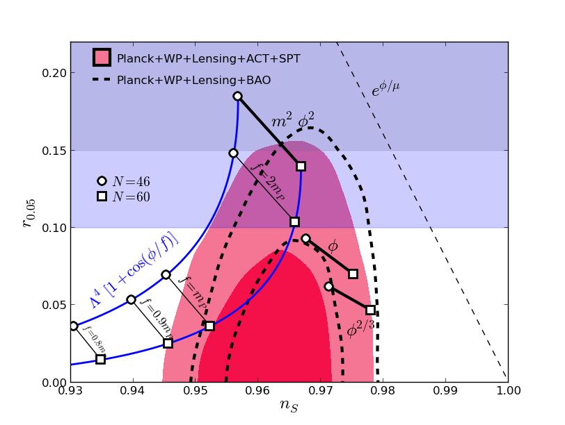
Figure 1: Original Natural Inflation (Cosine Potential): The band between the (solid/blue) lines running from approximately the lower left up to the middle of the plot are predictions for Natural Inflation for constant $N$ and varying $f$, where $N$ is the number of e-foldings prior to the end of inflation at which current modes of scale $k=0.002$ Mpc^-1 were generated and $f$ is the width of the potential. The range of values of $N$ reflect uncertainties in reheating after inflation as described in the text. Filled red (nearly vertical) regions are the parameter spaces allowed by Planck plus other CMB data as indicated at 68% and 95% C.L.’s. Dotted regions are the parameter spaces allowed by Planck + WMAP Polarization + Lensing +BAO at 68% and 95% C.L.’s. Horizontal blue bands correspond to 1(2) $\sigma$ measurements of $r$ from BICEP2 for the case of no running. The predictions match the data for trans-Planckian $f$. Also shown are the axion monodromy potential $V\propto\phi^{2/3}$ and the linear potential $V\propto\phi$, which are inconsistent with the BICEP2 limit at $2\sigma$, and the power-law inflationary potential $V\propto\exp{\left(\phi/\mu\right)}$ .

I Introduction

In a paper published in 1981, Guth proposed inflation Guth (1981) to solve several cosmological puzzles: an early period of accelerated expansion explains the homogeneity, isotropy, and flatness of the universe, as well as the lack of relic monopoles. Subsequently, Linde Linde (1982), as well as Albrecht and Steinhardt Albrecht and Steinhardt (1982) suggested rolling scalar fields as a mechanism to drive the dynamics of inflation (see Kazanas (1980); Starobinsky (1980); Sato (1981a, b); Mukhanov and Chibisov (1981); Mukhanov (2003); Linde (1983) for important early work). While inflation results in an approximately homogeneous universe, inflation models also predict small inhomogeneities. Observations of inhomogeneities via the cosmic microwave background (CMB) anisotropies and structure formation provide strong tests of inflation models.

In 1990, Freese, Frieman, and Olinto proposed the paradigm of natural inflation Freese et al. (1990) to solve theoretical problems of rolling inflation models. Most inflation models suffer from a potential drawback: to match various observational constraints, namely CMB anisotropy measurements and the requirement of sufficient inflation, the height of the inflaton potential must be of a much smaller scale than that of the width, by many orders of magnitude (i.e., the potential must be very flat). This requirement of two very different mass scales is what is known as the “fine-tuning” problem in inflation, since very precise couplings are required in the theory to prevent radiative corrections from bringing the two mass scales back to the same level. The natural inflation model (NI) uses shift symmetries to generate a flat potential, protected from radiative corrections, in a natural way Freese et al. (1990).

Natural inflation models use “axions” as the inflaton, the field responsible for inflation, where the term “axion” is used loosely for a field which has a flat potential as a result of a shift symmetry, i.e. the potential is unchanged under the transformation $\phi\rightarrow\phi+{\rm constant}$. During the early Universe, the inflaton field rolls along this flat potential for a long time, giving rise to the long period of inflationary expansion that solves the cosmological problems described above. Of course the shift symmetry must eventually be broken to allow the inflaton to roll to a minimum of the potential and inflationary expansion to proceed and finally stop. In this sense the inflaton in NI is an “axion,” or a “pseudo-Nambu-Goldstone boson,” with a nearly flat potential, exactly as required by inflation.

In the original natural inflation model proposed in 1990, the inflaton was directly modeled after the QCD axion, though with different mass scales. In this original model, the shape of the potential is a cosine, exactly as for the QCD axion. To match CMB observations, the height of the potential in the original Cosine NI is required to be $\sim 10^{16}$ GeV while the width is required to be $\lower 2.0pt\hbox{$\,\buildrel\scriptstyle>\over{\scriptstyle\sim}\,$}10^{19}$ GeV, as we will see in detail later in the paper. In 1995, WHK and K.T. Mahanthappa considered NI potentials generated by radiative corrections in models with explicitly broken Abelian Kinney and Mahanthappa (1995) and non-abelian Kinney and Mahanthappa (1996) symmetries. We will call these models KM Natural Inflation. Since that time many other variants of natural inflation have been proposed. A notable example is axion monodromy, where an axion arising in string compactification is the inflaton; the potential in this case is not periodic and instead can be linear or increasing as $\phi^{2/3}$. Remarkably, the data are now of sufficient accuracy to differentiate between these different types of NI models.

Over the past decade Cosmic Microwave Background (CMB) observations have confirmed basic predictions of inflation and are in addition providing stringent tests of individual inflationary models. First, generic predictions of inflation match the observations: the universe has a critical density ($\Omega=1$), the density perturbation spectrum is nearly scale invariant, and superhorizon fluctuations are evident. Second, current data differentiate between inflationary models and rule some of them out Spergel et al. (2007); Alabidi and Lyth (2006a); Peiris and Easther (2006a); Easther and Peiris (2006); Seljak et al. (2006); Kinney et al. (2006); Martin and Ringeval (2006); Martin et al. (2013, 2014); Peiris and Easther (2006b). For example, quartic potentials and generic tree-level hybrid models were disfavored already by WMAP data. The Planck satellite data has produced powerful tests of single-field rolling models Ade et al. (2013a). It has placed strong bounds on non-Gaussianity of the data, ruling out many non-minimal models including variants with multiple fields, non-canonical kinetic terms, and non-Bunch-Davies vacua Ade et al. (2013b). To quote the Planck team, “With these results, the paradigm of standard single-field inflation has survived its most stringent tests to date.”

Most recently, BICEP2 has made a ground-breaking discovery Ade et al. (2014). In addition to density perturbations, quantum fluctuations in inflation should produce gravitational waves that would appear as B-modes in polarization data. BICEP2 reported the first discovery of these gravity waves. They find that the observed B-mode power spectrum is well- fit by a lensed $\Lambda$-CDM + tensor theoretical model with tensor/scalar ratio $r=0.20^{+0.07}_{-0.05}$, with the null hypothesis disfavored at 7.0 $\sigma$. Alternatively, if running of the spectral index is allowed, the combined Planck and BICEP data could have a different best fit. In this paper we restrict our studies to the case of no running, consistent with the predictions of the simplest Natural Inflation models. Thus we will take as our lower bound on $r$:

$$r>0.15\ {\mathrm{at}}\ 1\sigma\ {\mathrm{and}}\ r>0.1\ {\mathrm{at}}\ 2\sigma.$$ (1)

It is the purpose of this paper to test natural inflation models with the Planck and BICEP2 data.

For comparison with the approach of taking the lower bound on $r$ from BICPE2, we also perform a joint likelihood analysis of Planck and BICEP2 (including data from some other experiments as described below). We compare the predictions of the Cosine NI model with the 68% and 95% confidence level regions of this joint likelihood analysis.

Inflation models predict two types of perturbations, scalar and tensor, which result in density and gravitational wave fluctuations, respectively. Each is typically characterized by a fluctuation amplitude ($P_{\mathcal{R}}^{1/2}$ for scalar and $P_{T}^{1/2}$ for tensor, with the latter usually given in terms of the ratio $r\equiv P_{T}/P_{\mathcal{R}}$) and a spectral index ($n_{s}$ for scalar and $n_{\textrm{T}}$ for tensor) describing the mild scale dependence of the fluctuation amplitude. The amplitude $P_{\mathcal{R}}^{1/2}$ is normalized by the height of the inflationary potential. The inflationary consistency condition $r=-8n_{\textrm{T}}$ further reduces the number of free parameters to two, leaving experimental limits on $n_{s}$ and $r$ as the primary means of distinguishing among inflation models. Hence, predictions of models are presented as plots in the $r$-$n_{s}$ plane.

The amplitude of the gravity waves and hence the value of $r$ is determined by the height of the potential, i.e., the energy scale of inflation. The relationship is given by

$$V=(2.2\times 10^{16}{\rm GeV})^{4}\frac{r}{0.2}.$$ (2)

Thus the BICEP2 bound $r>0.1$ at 2$\sigma$ requires the height of the potential to be at least $10^{16}$ GeV. Inflation is probing the GUT scale. Further, the width of the potential must exceed the the well-known Lyth Bound for single-field inflation Lyth (1997), which relates the tensor/scalar ratio to the field excursion $\Delta\phi$ during inflation,

$$\Delta\phi\geq m_{\textrm{Pl}}\sqrt{\frac{r}{4\pi}}.$$ (3)

With $r\sim 0.2$, inflation potentially becomes an interesting test of physics beyond the Planck scale.

The major results of this paper can be seen in Figures 1-5. The predictions of natural inflation models are plotted in the $r$-$n_{s}$ plane and compared to data from the Planck and BICEP2/Keck data. The predictions are plotted for various parameters: the width $f$ of the potential and number of e-foldings $N$ before the end of inflation at which present day fluctuation modes of scale $k=0.002$ Mpc^-1 were produced. $N$ depends upon the post-inflationary universe and is $\sim 46-60$. Also shown in the figure are the observational constraints from Planck and BICEP2. Figures 1-4 apply the lower bound on $r$ in Eqn(1). Figure 1 shows the original Cosine NI model; Figure 2 the KM NI model, and Figure 3 summarizes a variety of potentials. Figure 4 shows a Higgs potential for comparison. In Figure 5 (for comparison with Figure 1), we plot the predictions of the Cosine NI model vs. the 68% and 95% confidence level regions of the joint likelihood analysis of Planck and BICEP2 data. Our primary result is that the original Natural Inflation Model and KM NI are consistent with current observational constraints.

In this paper we take $m_{\textrm{Pl}}=1.22\times 10^{19}$ GeV. Our result extends upon previous analyses of NI Freese and Kinney (2004) and Savage et al. (2006) that was based upon WMAP’s first year data Spergel et al. (2003) and third year data. Even earlier analyses Adams et al. (1993); Moroi and Takahashi (2001) placed observational constraints on this model using COBE data Smoot et al. (1992). Other papers have studied inflation models (including NI) in light of the WMAP1 and WMAP3 data Alabidi and Lyth (2006a, b) and in light of Planck data Tsujikawa et al. (2013).

In previous papers Savage et al. (2006) Freese et al. (2008), we found how far down the potential the field is at the time structure is produced, and found that for $f\gg m_{\textrm{Pl}}$ the relevant part of the potential is indistinguishable from a quadratic potential (yet has the advantage that the required flatness is well- motivated). Indeed one can see that $V\sim m^{2}\phi^{2}$ matches all the data. We will examine one other model with a GUT-scale Higgs-like potential, and show that it too can match the data. The BICEP2 data have substantially reduced the number of inflationary models that agree with data.

We will begin by discussing the model of natural inflation in Section II: the motivation, the potential, and relating pre- and post-inflation scales. We will describe which of the natural inflation models we plan to compare to data. In Section III, we will examine the scalar and tensor perturbations predicted by NI models and compare them with Planck and BICEP2 data in Section IV. We conclude in Section V.

II The Model of Natural Inflation

II.1 Motivation

To satisfy a combination of constraints on inflationary models, in particular, sufficient inflation and microwave background anisotropy measurements Spergel et al. (2003, 2007), the potential for the inflaton field must be very flat. For a general class of inflation models involving a single slowly-rolling field, it has been shown that the ratio of the height to the (width)⁴ of the potential must satisfy Adams et al. (1991)

$$\chi\equiv\Delta V/(\Delta\phi)^{4}\leq{\cal O}(10^{-6}-10^{-8})\,,$$ (4)

where $\Delta V$ is the change in the potential $V(\phi)$ and $\Delta\phi$ is the change in the field $\phi$ during the slowly rolling portion of the inflationary epoch. Thus, the inflaton must be extremely weakly self-coupled, with effective quartic self-coupling constant $\lambda_{\phi}<\mathcal{O}(\chi)$ (in realistic models, $\lambda_{\phi}<10^{-12}$). The small ratio of mass scales required by Eq. (4) quantifies how flat the inflaton potential must be and is known as the “fine-tuning” problem in inflation. Reviews of inflation can be found in Ref. Bassett et al. (2006); Kinney (2009); Baumann (2009).

Three approaches have been taken toward this required flat potential characterized by a small ratio of mass scales. First, some simply say that there are many as yet unexplained hierarchies in physics, and inflation requires another one. The hope is that all these hierarchies will someday be explained. In these cases, the tiny coupling $\lambda_{\phi}$ is simply postulated ad hoc at tree level, and then must be fine-tuned to remain small in the presence of radiative corrections. But this merely replaces a cosmological naturalness problem with unnatural particle physics. Second, models have been attempted where the smallness of $\lambda_{\phi}$ is protected by supersymmetry. Even if such a model succeeded (most suffer from the famous $\eta$-problem), the required mass hierarchy, while stable, is itself unexplained. It would be preferable if such a hierarchy, and thus inflation itself, arose dynamically in particle physics models.

Hence, in 1990 a third approach was proposed, Natural Inflation Freese et al. (1990), in which the inflaton potential is flat due to shift symmetries. The original model followed the physics of the QCD axion though later variants have generalized. The potential is exactly flat due to a shift symmetry under $\phi\rightarrow\phi+\textrm{ constant}$. As long as the shift symmetry is exact, the inflaton cannot roll and drive inflation, and hence there must be additional explicit symmetry breaking. Then these particles become pseudo-Nambu Goldstone bosons (PNGBs), with nearly flat potentials, exactly as required by inflation. The small ratio of mass scales required by Eq. (4) can easily be accommodated. For example, in the case of the QCD axion, this ratio is of order $10^{-64}$. While inflation clearly requires different mass scales than the axion, the point is that the physics of PNGBs can easily accommodate the required small numbers.

The NI model was first proposed and a simple analysis performed in Freese et al. (1990). Then, in 1993, a second paper followed which provides a much more detailed study Adams et al. (1993). Many types of candidates have subsequently been explored for natural inflation. For example, WHK and K.T. Mahanthappa considered NI potentials generated by radiative corrections in models with explicitly broken Abelian Kinney and Mahanthappa (1995) and non-abelian Kinney and Mahanthappa (1996) symmetries. We will mention a few others.

We will see that cosine NI requires the width of the potential to be trans-Planckian. Such a scenario is difficult to accommodate in string theory. Thus many authors have proposed other variants of NI, taking advantage of the shift symmetry offered by ”axions,” and looking for extensions of the original cosine potential that accommodate smaller values of $f$. Kim, Nilles & Peloso Kim et al. (2005) as well as the idea of N-flation Dimopoulos et al. (2008); Grimm (2008) generalized the original NI model to include two or more axions, and showed that an effective potential of $f\gg m_{\textrm{Pl}}$ can be generated from multiple axions, each with sub-Planckian scales. Ref. Kawasaki et al. (2000) used shift symmetries in Kahler potentials to obtain a flat potential and drive natural chaotic inflation in supergravity. Additionally, Arkani-Hamed et al. (2003a, b) examined natural inflation in the context of extra dimensions and Kaplan and Weiner (2004) used PNGBs from little Higgs models to drive hybrid inflation. Also, Firouzjahi and Tye (2004); Hsu and Kallosh (2004) use the natural inflation idea of PNGBs in the context of braneworld scenarios to drive inflation. Freese Freese (1994) suggested using a PNGB as the rolling field in double field inflation Adams and Freese (1991) (in which the inflaton is a tunneling field whose nucleation rate is controlled by its coupling to a rolling field). Ref. Kaloper and Sorbo (2009); Kaloper et al. (2011) found a quadratic potential in theories where an ”axion” field mixes with a 4-form. Ref. Germani and Kehagias (2011); Germani and Watanabe (2011) used coupling of the inflaton kinetic term to the Einstein tensor to allow NI with $f<<m_{pl}$ by enhancing the gravitational friction acting on the inflaton during inflation. Ref. Czerny and Takahashi (2014); Czerny et al. (2014) suggested a ”multi-natural” inflation model in which the single-field inflaton potential consists of two or more sinusoidal potentials with a possible non-zero relative phase (such as may arise if a complex scalar field is coupled to two sets of quark and anti- quark fields). We will focus in this paper on single field implementations of NI.

II.2 Potential

We present a variety of natural inflation potentials. The feature they all share is a shift symmetry that maintains the required flatness of the potential.

II.2.1 Original Natural Inflation (Cosine Potential)

In the original natural inflation model, modeled after the QCD axion, the PNGB potential resulting from explicit breaking of a shift symmetry is of the form

$$V(\phi)=\Lambda^{4}[1\pm\cos(N\phi/f)]\,.$$ (5)

We will take the positive sign in Eq. (5) (this choice has no effect on our results) and take $N=1$, so the potential, of height $2\Lambda^{4}$, has a unique minimum at $\phi=\pi f$ (the periodicity of $\phi$ is $2\pi f$).

For appropriately chosen values of the mass scales, e.g. $f\lower 2.0pt\hbox{$\,\buildrel\scriptstyle>\over{\scriptstyle\sim}\,$}m_{\textrm{Pl}}$ and $\Lambda\sim m_{\textrm{GUT}}\sim 10^{16}$ GeV, the PNGB field $\phi$ can drive inflation. This choice of parameters indeed produces the small ratio of scales required by Eq. (4), with $\chi\sim(\Lambda/f)^{4}\sim 10^{-13}$. For $\Lambda\sim 10^{15}$-$10^{16}$ GeV we have $f\sim m_{\textrm{Pl}}$, yielding an inflaton mass $m_{\phi}=\Lambda^{2}/f\sim 10^{11}$-$10^{13}$ GeV. For $f\gg m_{\textrm{Pl}}$, the inflaton becomes independent of the scale $f$ and is $m_{\phi}\sim 10^{13}$ GeV.

II.2.2 Low-scale inflation

It is possible that the shift symmetry responsible for providing the stability of the mass hierarchy in NI is respected to such a degree that the mass term for the inflaton is identically zero. In such a case, an effective expansion for the inflaton potential can be written

$$V\left(\phi\right)=V_{0}-\sum_{p}{\lambda_{p}\left(\frac{\phi}{\mu}\right)^{p}},$$ (6)

where the leading order operator for $\phi\ll\mu$ is of order $p>2$. In this case, a remarkable cancellation occurs, such that the spectral index is independent of the mass scales in the potential, and depends only on the number of e-folds of inflation Kinney and Mahanthappa (1996),

$$n_{s}-1=-\left(\frac{2}{N}\right)\frac{p-1}{p-2},$$ (7)

where $N\sim 60$ is the number of e-folds before the end of inflation. For $N=[46,60]$, consistent with a reheat temperature above $1\ {\rm TeV}$, and assuming an even exponent $p\geq 4$, the scalar spectral index is confined to a narrow range, $n_{s}=[0.935,0.967]$, which overlaps nicely with the region favored by Planck. Because the spectral index is independent of the scales in the potential, such models can successfully generate inflation for $\mu\ll m_{\rm Pl}$. Figure 2 shows the predictions of various low-scale models relative to Planck and BICEP. Such models with $\mu<m_{\rm Pl}$ are strongly ruled out by the tensor mode detection of BICEP.

In 1995, Kinney and Mahanthappa proposed a realization of such low-scale inflation scenarios in which the inflaton potential is generated by radiative corrections in an explicitly broken SO(3) gauge symmetry. In this scenario, the inflaton is a pseudo-Goldstone mode with potential

$$V=V_{0}\left\{\sin^{4}\left(\frac{\phi}{\mu}\right)\log\left[g^{2}\sin^{2}\left(\frac{\phi}{\mu}\right)\right]-\log\left[g^{2}\right]\right\}.$$ (8)

In the low-scale limit $\mu\ll m_{\textrm{Pl}}$, such potentials reduce to the quartic hilltop type at leading order in a Taylor expansion,

$$V\simeq V_{0}-\lambda\left(\frac{\phi}{\mu}\right)^{4}+\cdots$$ (9)

The low-scale limit of these models is inconsistent with the data, but extension of the model to large field values, $\mu>m_{\rm Pl}$ is possible, and is still consistent with the BICEP2 data. Figure 3 shows this model relative to the Planck and BICEP2 constraints.

II.2.3 String-motivated Axion Potentials

Axion monodromy Silverstein and Westphal (2008) is a shift-symmetric string-motivated version of Natural Inflation which evades the super-Planck scale width of the cosine potential by analytic continuation on a compact manifold, resulting in an effective field range larger than $m_{\textrm{Pl}}$. A resulting potential $V\propto\phi^{2/3}$ is inconsistent with the BICEP2 data at $2\sigma$. Linear Axion Monodromy McAllister et al. (2010) with $V\propto\phi$ is also inconsistent with BICEP2 to $2\sigma$. Versions of axion monodromy with additional couplings to heavy degrees of freedom can produce larger tensor amplitudes Dong et al. (2011), consistent with BICEP2.

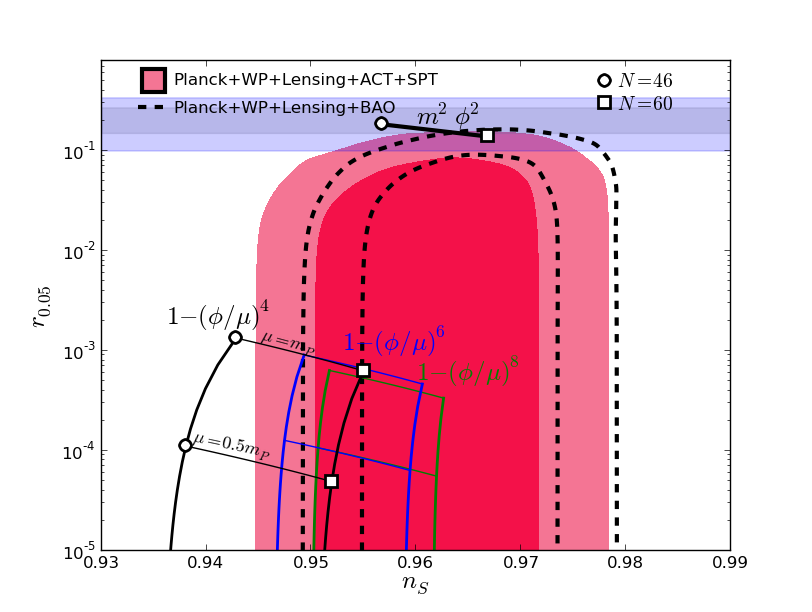
Figure 2: Low-scale models of natural inflation Low-scale models with $\mu<m_{\rm Pl}$ are shown relative to the constraints from Planck and BICEP2. These models are strongly ruled out by the BICEP2 detection of tensor modes. Labels same as in Figure 1 (roughly, solid lines are theoretical predictions; red is Planck data; blue is BICEP2 data).

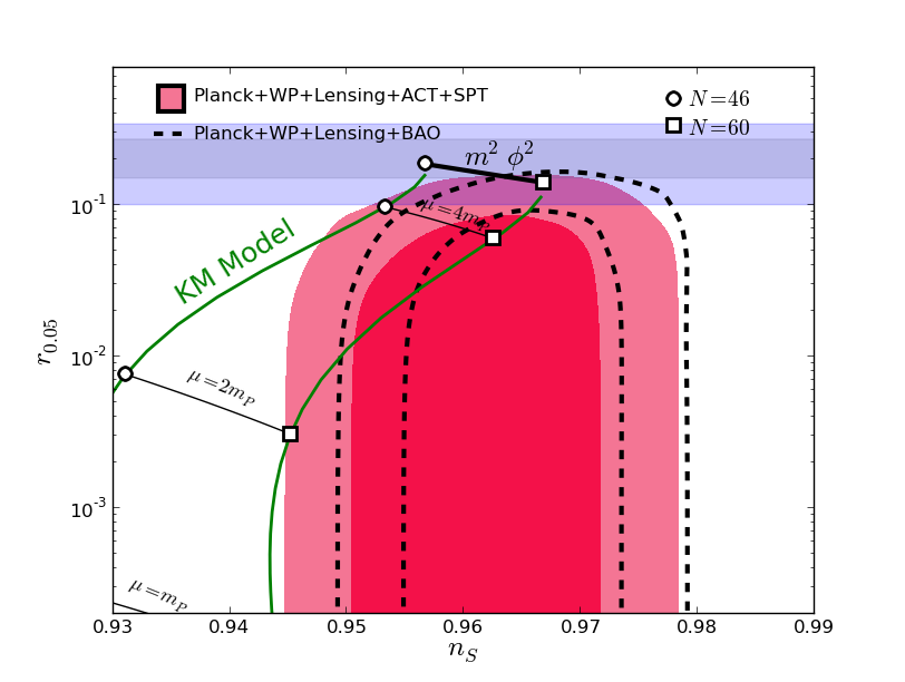
Figure 3: KM Model of natural inflation Labels same as in Figure 1 (roughly, solid lines are theoretical predictions; red is Planck data; blue is BICEP2 data).

II.3 Relating Pre- and Post-Inflation Scales

To test inflationary theories, present day observations must be related to the evolution of the inflaton field during the inflationary epoch. Here we show how a comoving scale $k$ today can be related back to a point during inflation. We need to find the value of $N_{k}$, the number of e-foldings before the end of inflation, at which structures on scale $k$ were produced.

Under a standard post-inflation cosmology, once inflation ends, the universe undergoes a period of reheating. Reheating can be instantaneous or last for a prolonged period of matter-dominated expansion. Then reheating ends at $T<T_{\textrm{RH}}$, and the universe enters its usual radiation-dominated and subsequent matter-dominated history. Instantaneous reheating ($\rho_{\textrm{RH}}=\rho_{e}$) gives the minimum number of e-folds as one looks backwards to the time of perturbation production, while a prolonged period of reheating gives a larger number of e-folds.

The relationship between scale $k$ and the number of e-folds $N_{k}$ before the end of inflation has been shown to be Lidsey et al. (1997)

$$N_{k}=62-\ln\frac{k}{a_{0}H_{0}}-\ln\frac{10^{16}\,\textrm{GeV}}{V_{k}^{1/4}}+\ln\frac{V_{k}^{1/4}}{V_{\textrm{e}}^{1/4}}-\frac{1}{3}\ln\frac{V_{\textrm{e}}^{1/4}}{\rho_{\textrm{RH}}^{1/4}}\,.$$ (10)

Here, $V_{k}$ is the potential when $k$ leaves the horizon during inflation, $V_{\textrm{e}}=V(\phi_{\textrm{e}})$ is the potential at the end of inflation, and $\rho_{\textrm{RH}}$ is the energy density at the end of the reheat period. Nucleosynthesis generally requires $\rho_{\textrm{RH}}\lower 2.0pt\hbox{$\,\buildrel\scriptstyle>\over{\scriptstyle\sim}\,$}(\textrm{1 GeV})^{4}$, while necessarily $\rho_{\textrm{RH}}\leq V_{\textrm{e}}$. Since $V_{\textrm{e}}$ may be of order $m_{\textrm{GUT}}\sim 10^{16}$ GeV or even larger, there is a broad allowed range of $\rho_{\textrm{RH}}$; this uncertainty in $\rho_{\textrm{RH}}$ translates into an uncertainty of 10 e-folds in the value of $N_{k}$ that corresponds to any particular scale of measurement today.

Henceforth we will use $N$ to refer to the number of e-foldings prior to the end of inflation that correspond to scale $k=0.002$ Mpc^-1. Under the standard cosmology, this scale corresponds to $N\sim$46-60 (smaller $N$ corresponds to smaller $\rho_{\textrm{RH}}$), with a slight dependence on $f$.

III Perturbations

As the inflaton rolls down the potential, quantum fluctuations lead to metric perturbations that are rapidly inflated beyond the horizon. These fluctuations are frozen until they re-enter the horizon during the post-inflationary epoch, where they leave their imprint on large scale structure formation and the cosmic microwave background (CMB) anisotropy Guth and Pi (1982); Hawking (1982); Starobinsky (1982).

III.1 Scalar (Density) Fluctuations

The perturbation amplitude for the density fluctuations (scalar modes) produced during inflation is given by Mukhanov (1985, 1988); Mukhanov et al. (1992); Stewart and Lyth (1993)

$$P_{\mathcal{R}}^{1/2}(k)=\frac{H^{2}}{2\pi\dot{\phi}_{k}}\,.$$ (11)

Here, $P_{\mathcal{R}}^{1/2}(k)\sim\frac{\delta\rho}{\rho}|_{\textrm{hor}}$ denotes the perturbation amplitude when a given wavelength re-enters the Hubble radius in the radiation- or matter-dominated era, and the right hand side of Eq. (11) is to be evaluated when the same comoving wavelength ($2\pi/k$) crosses outside the horizon during inflation.

Normalizing to the COBE Smoot et al. (1992) or WMAP Spergel et al. (2007) anisotropy measurements gives $P_{\mathcal{R}}^{1/2}\sim 10^{-5}$. This normalization can be used to approximately fix the height $\Lambda$ of the potential Eq. (5). The largest amplitude perturbations on observable scales are those produced $N\sim 60$ e-folds before the end of inflation (corresponding to the horizon scale today), when the field value is $\phi=\phi_{N}$. For cosine Natural Inflation, under the SR approximation, the amplitude on this scale takes the value

$$P_{\mathcal{R}}\approx\frac{128\pi}{3}\left(\frac{\Lambda}{m_{\textrm{Pl}}}\right)^{4}\left(\frac{f}{m_{\textrm{Pl}}}\right)^{2}\frac{[1+\cos(\phi_{N}/f)]^{3}}{\sin^{2}(\phi_{N}/f)}\,.$$ (12)

The fluctuation amplitudes are, in general, scale dependent. The spectrum of fluctuations is characterized by the spectral index $n_{s}$,

$$n_{s}-1\equiv\frac{\mathrm{d}\ln P_{\mathcal{R}}}{\mathrm{d}\ln k}\approx-\frac{1}{8\pi}\left(\frac{m_{\textrm{Pl}}}{f}\right)^{2}\frac{3-\cos(\phi/f)}{1+\cos(\phi/f)}\,.$$ (13)

For small $f$, $n_{s}$ is essentially independent of $N$, while for $f\lower 2.0pt\hbox{$\,\buildrel\scriptstyle>\over{\scriptstyle\sim}\,$}2m_{\textrm{Pl}}$, $n_{s}$ has essentially no $f$ dependence. Analytical estimates can be obtained in these two regimes:

$$n_{s}\approx\begin{cases}1-\frac{m_{\textrm{Pl}}^{2}}{8\pi f^{2}}\,,&\textrm{for}\,\,f\lower 2.0pt\hbox{$\,\buildrel\scriptstyle<\over{\scriptstyle\sim}\,$}\frac{3}{4}m_{\textrm{Pl}}\\ 1-\frac{2}{N}\,,&\textrm{for}\,\,f\lower 2.0pt\hbox{$\,\buildrel\scriptstyle>\over{\scriptstyle\sim}\,$}2m_{\textrm{Pl}}\,.\end{cases}$$ (14)

For $f\lower 2.0pt\hbox{$\,\buildrel\scriptstyle>\over{\scriptstyle\sim}\,$}m_{pl}$, natural inflation predicts a small, $O(10^{-3}$), negative spectral index running. This small running is a prediction of the model.

The Planck results as shown in Figure 1 led to the constraint $f\lower 2.0pt\hbox{$\,\buildrel\scriptstyle>\over{\scriptstyle\sim}\,$}0.8m_{\textrm{Pl}}$ at 95% C.L. With the inclusion of BICEP2 data, the bound becomes stronger and $f$ must be trans-Planckian.

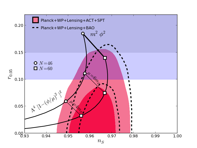
Figure 4: Higgs-like inflation. Labels same as in Figure 1 (roughly, solid lines are theoretical predictions; red is Planck data; blue is BICEP2 data).

III.2 Tensor (Gravitational Wave) Fluctuations

In addition to scalar (density) perturbations, inflation also produces tensor (gravitational wave) perturbations with amplitude

$$P_{T}^{1/2}(k)=\frac{4H}{\sqrt{\pi}m_{\textrm{Pl}}}\,.$$ (15)

As mentioned in the introduction, the amplitude of the gravity waves is directly proportional to the Hubble parameter and therefore is determined by the energy scale of the height of the potential.

Conventionally, the tensor amplitude is given in terms of the tensor/scalar ratio

$$r\equiv\frac{P_{T}}{P_{\mathcal{R}}}=16\epsilon\,,$$ (16)

For small $f$, $r$ rapidly becomes negligible, while $f\to\frac{8}{N}$ for $f\gg m_{\textrm{Pl}}$.

As mentioned in the introduction, in principle, there are four parameters describing scalar and tensor fluctuations: the amplitude and spectra of both components, with the latter characterized by the spectral indices $n_{s}$ and $n_{\textrm{T}}$ (we are ignoring any running here). The amplitude of the scalar perturbations is normalized by the height of the potential (the energy density $\Lambda^{4}$). The tensor spectral index $n_{\textrm{T}}$ is not an independent parameter since it is related to the tensor/scalar ratio $r$ by the inflationary consistency condition $r=-8n_{\textrm{T}}$. The remaining free parameters are the spectral index $n_{s}$ of the scalar density fluctuations, and the tensor amplitude (given by $r$). Hence, a useful parameter space for plotting the model predictions versus observational constraints is on the $r$-$n_{s}$ plane Dodelson et al. (1997); Kinney (1998).

The Planck constraints are generated using the COSMOMC Markov Chain Monte Carlo code Lewis and Bridle (2002), marginalizing over a seven-parameter data set with flat priors:

• Dark Matter density $\Omega_{\rm M}h^{2}$.

• Baryon density $\Omega_{\rm b}h^{2}$.

• Reionization optical depth $\tau$.

• The angular size $\theta$ of the sound horizon at decoupling.

• Scalar spectrum normalization $A_{\rm S}$.

• Tensor/scalar ratio $r$.

• Scalar spectral index $n_{s}$.

The fit assumes a flat universe $\Omega_{\rm b}+\Omega_{\rm M}+\Omega_{\rm\Lambda}=1$, with Cosmological Constant Dark Energy, $\rho_{\Lambda}={\rm const.}$ Convergence is determined via a Gelman and Rubin statistic. Auxiliary data sets used are WMAP polarization (WP), in combination with the Atacama Cosmology Telescope (ACT) / South Pole Telescope (SPT) CMB measurements (solid contours in figures), and Baryon Acoustic Oscillation (BAO) data from Sloan Digital Sky Survey Data Release 9 Ahn et al. (2012), the 6dF Galaxy Survey Jones et al. (2009), and the WiggleZ Dark Energy Survey Blake et al. (2011) (dashed contours).

The BICEP2 allowed region is taken from Ref. Ade et al. (2014) as $r=0.2^{+0.07}_{-0.05}$. We plot this as a one-sigma (dark-) and two-sigma (light-) shaded region, separately from the Planck contours, which illustrates two important points: First BICEP2 alone does not provide constraint on the spectral index of scalar perturbations, since it only measures the amplitude of the tensor signal. Second, there is clearly tension between the BICEP2 constraint on the tensor/scalar ratio $r$ and the Planck constraint with no running of the spectral index, which sets a 95%-confidence upper limit of $r<0.17$ Ade et al. (2013a). While Planck and BICEP2 are consistent at the $2\sigma$ confidence level, they are significantly discrepant at the $1\sigma$ level. For comparison, a joint likelihood for Planck and BICEP is shown in Figure 5. The BICEP2 contours are sensitive to the details of foreground removal Ade et al. (2014), which may help lower the best-fit $r$ slightly, and at least partially resolve the tension with Planck. Other possibilities for resolving the tension are an extra neutrino species Giusarma et al. (2014), or running of the spectral index Ade et al. (2014) (the latter would invalidate all of the models considered here). For the purposes of this paper, we take the quoted best-fit region for BICEP2 at face value, and investigate its implications.

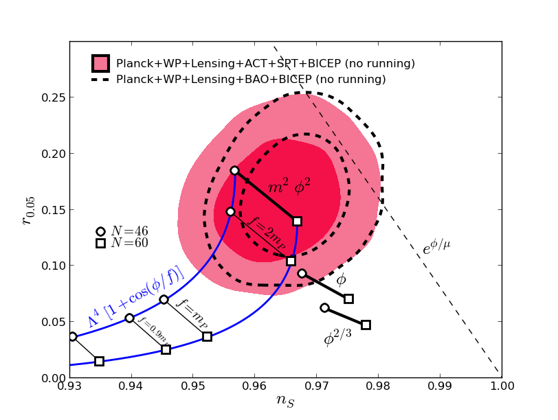
Figure 5: Cosine Natural Inflation: Joint likelihood for Planck + WMAP Polarization + Lensing + BICEP, including ACT/SPT and BAO, for comparison with Figure 1. Inner contours are 68 % confidence limits, outer contours are 95 % confidence. Note that the linear potential $V\propto\phi$ is marginally consistent with the joint fit at 95% confidence, as is the power-law potential $V\propto e^{\phi/\mu}$.

IV Results

In Figure 1, we show the predictions of the original natural inflation model together with the observational constraints. Parameters corresponding to fixed $N$= 46 and 60 with varying $f$ are shown as (solid/blue) lines from the lower left to upper right. The orthogonal (black) lines correspond to fixed $f$ with varying $N$. The band between the blue lines are the values of $N$ consistent with standard post-inflation cosmology for reheat temperatures above the nucleosynthesis limit of $\sim$1 GeV, as discussed previously. The solid red regions are the allowed parameters at 68% and 95% C.L.’s from Planck + other CMB data. The blue regions are the parameters at 1 and 2 $\sigma$ consistent with the BICEP2 discovery of B modes. For a given $N$, a fixed point is reached for $f\gg m_{\textrm{Pl}}$; that is, $r$ and $n_{s}$ become essentially independent of $f$ for any $f\gg m_{\textrm{Pl}}$, and Natural Inflation becomes equivalent to a large-field $m^{2}\phi^{2}$ model (note, however, that in natural inflation this effectively power law potential is produced via a natural mechanism). As seen in the figure, $f\lower 2.0pt\hbox{$\,\buildrel\scriptstyle<\over{\scriptstyle\sim}\,$}m_{\textrm{Pl}}$ is excluded. However, $f\lower 2.0pt\hbox{$\,\buildrel\scriptstyle>\over{\scriptstyle\sim}\,$}m_{\textrm{Pl}}$ falls well into the allowed region and is thus consistent with all data. Figure 1 also shows the axion monodromy potential with $V\sim\phi^{2/3}$, which is inconsistent with the BICEP2 constraint. Linear potentials $V\propto\phi$ are inconsistent with the BICEP2 limit at the 95% confidence level, but are marginally consistent with a joint Planck/BICEP2 limit at 95%, as is the power-law potential $V\propto e^{\phi/\mu}$.

In Figure 3 we show the predictions of KM inflation and compare them to all data sets. There is some tension in obtaining high enough values of $r$ in these models.

In Figure 2 we plot the results for a variety of potentials for low-scale inflation models of the form $V(\phi)\propto 1-(\phi/\mu)^{p}$ with $p\lower 2.0pt\hbox{$\,\buildrel\scriptstyle>\over{\scriptstyle\sim}\,$}4$. These models would have had low scales; the energy scale of the potentials as well as their widths could have been much lower than for the cosine model. However, these low scales correspond to low values of $r$ and are ruled out by the BICEP2 data.

For comparison, in Figure 4 we study a Higgs-like potential, which has no connection to natural inflation. The potential is that of a Higgs-like particle at the GUT scale, with potential

$$V\left(\phi\right)=V_{0}\left[1-\left(\frac{\phi}{\mu}\right)^{2}\right]^{2}$$ (17)

One can see that such a potential remains a good fit to the data as well, as long as the mass scales are high.

In Figure 5, we compare the predictions of the cosine Natural Inflation model vs. the joint likelihood for Planck + WMAP Polarization + Lensing + BICEP, including ACT/SPT and BAO, for comparison with Figure 1. Inner contours are 68% confidence limits, outer contours are 95% confidence.

V Conclusion

Remarkable advances in cosmology have taken place in the past decade thanks to Cosmic Microwave Background experiments. The release of the BICEP2 data is revolutionary and will lead to even more exciting times for inflationary cosmology. The success of BICEP2 should motivate future missions even going to space. Not only have generic predictions of inflation been confirmed by a series of CMB experiments (though there are still outstanding theoretical issues), but indeed individual inflation models are being tested with large classes already ruled out.

Currently the natural inflation model, which is well-motivated on theoretical grounds of naturalness, is a good fit to existing data. In Figure 1, we showed that for the cosine potential with width $f\lower 2.0pt\hbox{$\,\buildrel\scriptstyle>\over{\scriptstyle\sim}\,$}m_{\textrm{Pl}}$ and height $\Lambda\sim m_{\textrm{GUT}}$ the model is in good agreement with all CMB data. Natural inflation predicts very little running, at the level of $10^{-3}$, and this will become a test of the model. Even for values $f\gg m_{\textrm{Pl}}$ where the relevant parts of the potential are indistinguishable from quadratic, natural inflation provides a framework free of fine-tuning for the required potential.

Other than natural inflation, single-field models compatible with all existing data sets include the $m^{2}\phi^{2}$ quadratic potential (to which natural inflation asymptotes for large $f$ as mentioned above) as well as the potential for a Higgs-like particle at the GUT scale (see Figure 4). The BICEP2 data have substantially reduced the number of inflationary models that agree with data.

In summary, Natural Inflation represents a model which is both well-motivated and testable. It is a good fit to all cosmic microwave background (CMB) data and may be the correct description of an early inflationary expansion of the Universe.