Fomalhaut b as a Cloud of Dust: Testing Aspects of Planet Formation Theory

Abstract

We consider the ability of three models – impacts, captures, and collisional cascades – to account for a bright cloud of dust in Fomalhaut b. Our analysis is based on a novel approach to the power-law size distribution of solid particles central to each model. When impacts produce debris with (i) little material in the largest remnant and (ii) a steep size distribution, the debris has enough cross-sectional area to match observations of Fomalhaut b. However, published numerical experiments of impacts between 100 km objects suggest this outcome is unlikely. If collisional processes maintain a steep size distribution over a broad range of particle sizes (300 $\rm\mu{\rm m}$ to 10 km), Earth-mass planets can capture enough material over 1–100 Myr to produce a detectable cloud of dust. Otherwise, capture fails. When young planets are surrounded by massive clouds or disks of satellites, a collisional cascade is the simplest mechanism for dust production in Fomalhaut b. Several tests using HST or JWST data – including measuring the expansion/elongation of Fomalhaut b, looking for trails of small particles along Fomalhaut b’s orbit, and obtaining low resolution spectroscopy – can discriminate among these models.

1 INTRODUCTION

Fomalhaut b is a faint object orbiting at a distance of $\sim$ 120 AU from the nearby A-type star Fomalhaut. Originally detected on Hubble Space Telescope (HST) images at 0.6 $\rm\mu{\rm m}$ and 0.8 $\rm\mu{\rm m}$ (Kalas et al., 2008), the source lies inside the orbits of a bright belt of dust particles at 130–150 AU from the central star (e.g., Holland et al., 2003; Stapelfeldt et al., 2004; Kalas et al., 2005; Marsh et al., 2005; Ricci et al., 2012; Acke et al., 2012; Boley et al., 2012; Su et al., 2013). Recent re-analyses of the original HST data confirm the detections at 0.6–0.8 $\rm\mu{\rm m}$ and identify the source on images at 0.435 $\rm\mu{\rm m}$ (Currie et al., 2012; Galicher et al., 2013). New optical HST data recover the object in 2010–2012 (Kalas et al., 2013). In all of these studies, the optical colors are similar to those of the central star.

Despite the robust optical data, Fomalhaut b is not detected at infrared (IR) wavelengths. Attempts to identify the source have failed at 1.25 $\rm\mu{\rm m}$ (Currie et al., 2012), 1.6 $\rm\mu{\rm m}$ (Kalas et al., 2008; Currie et al., 2013), 3.6–3.8 $\rm\mu{\rm m}$ (Kalas et al., 2008; Marengo et al., 2009), and 4.5 $\rm\mu{\rm m}$ (Marengo et al., 2009; Janson et al., 2012). Each upper limit lies well above the IR fluxes expected for an object with the optical-infrared colors of an A-type star. Although the brighter IR fluxes expected from a 2–10 $M_{\rm J}$ (Jupiter mass) planet are excluded by these data, the IR data are consistent with emission from lower mass planets (e.g., Janson et al., 2012; Currie et al., 2012). However, the measured optical fluxes in Fomalhaut b are a factor $\gtrsim$ 100 larger than expected for a 1 $M_{\rm J}$ planet at a distance of 7.7 pc from the Earth (e.g., Currie et al., 2012). Thus, the optical flux requires a different source.

Without a clear IR detection, the simplest explanation for the emission from Fomalhaut b is scattered light from an ensemble of dust grains with a collective cross-sectional area of roughly $10^{23}$ cm² (e.g., Kalas et al., 2008). A single, high velocity collision between two objects with radii of 10–1000 km is a plausible source for the dust (Wyatt & Dent, 2002; Kenyon & Bromley, 2005; Kalas et al., 2008; Galicher et al., 2013; Kalas et al., 2013). In this picture, the collision disperses objects with sizes ranging from a fraction of a micron to tens of meters or kilometers (see, for example, the discussions in Wyatt & Dent, 2002; Kenyon & Bromley, 2005).

A collisional cascade within a circumplanetary cloud (Kennedy & Wyatt, 2011) or debris disk (Kalas et al., 2008) is another plausible source of dust grains in Fomalhaut b (e.g., Currie et al., 2012; Galicher et al., 2013; Kalas et al., 2013). In this model, dynamical processes place a massive cloud of satellites around a newly-formed 1–100 $M_{\oplus}$ planet (e.g., Nesvorný et al., 2007). Subsequent collisions among 1–100 km satellites produce copious amounts of dust (e.g., Bottke et al., 2010; Kennedy & Wyatt, 2011). Aside from the nature of the collisions, this mechanism probably produces dust grains with properties similar to those derived from a single giant impact.

Material continuously captured from Fomalhaut’s circumstellar disk provides a third source for dust in Fomalhaut b. In this picture (e.g., Ruskol, 1961, 1963, 1972), material orbiting Fomalhaut loses energy and is captured by a massive planet. Collisions among captured objects produce a cloud of dust grains orbiting the planet. If the grains within this disk remain small, their properties are probably similar to dust produced in a single collision or in a collisional cascade.

In this paper, we develop a framework for analyzing dusty clouds of debris and apply this framework to available data for Fomalhaut b. We begin in §2 with a summary of relevant data for this system. In §3, we consider a novel approach for deriving properties of the debris from the observed cross-sectional area (§3.1) and apply this approach to dust produced in a giant impact (§3.2), captured from the protoplanetary disk (§3.3), and generated in a collisional cascade (§3.4). After exploring uncertainties, tests, and improvements of these mechanisms for dust production (§4), we conclude with a brief summary (§5).

2 RELEVANT OBSERVATIONS

To develop robust models for dust emission in Fomalhaut b, we first establish pertinent observational results from existing data. Fomalhaut is a 200–400 Myr old A3 V star at a distance, $D$ = 7.7 pc (e.g., Barrado y Navascues, 1998; Mamajek, 2012). The star has two nearby, apparently bound companions, TW PsA (K4 V) and LP 876-10 (M4 V), at distances 0.28–0.77 pc from the primary star (Barrado y Navascues, 1998; Mamajek, 2012; Mamajek et al., 2013). Fomalhaut and LP 876-10 have bright debris disks (Gillett, 1986; Kennedy et al., 2013). Fomalhaut b has an eccentric orbit (e $\approx$ 0.8) around Fomalhaut with a semimajor axis, $a_{b}\approx$ 160–180 AU (Kalas et al., 2013; Beust et al., 2014). This orbit might intersect the orbits of material in the outer debris belt of Fomalhaut (Kalas et al., 2013; Beust et al., 2014).

2.1 Fomalhaut Debris Disk

All three dust models depend on the amount of circumstellar material along Fomalhaut b’s orbit. The main belt at 130–150 AU lies outside the current position of Fomalhaut b (Kalas et al., 2005, 2013). Within the belt, the mass in solids is at least 20–40 $M_{\oplus}$ (e.g., Wyatt & Dent, 2002; Holland et al., 2003) and is probably less than 300 $M_{\oplus}$ (Kalas et al., 2013). Models which fit images and the spectral energy distribution suggest that the belt of dust at 130–155 AU contains roughly twice as much dust as the region from 35–130 AU (e.g., Acke et al., 2012). Accounting for the difference in surface area, the surface density of dust in the inner disk is roughly 15% of the surface density in the main belt.

To place these results in the context of planet formation theory, the surface density of a protoplanetary disk around Fomalhaut is conveniently parameterized as (e.g., Youdin & Kenyon, 2013):

$$\Sigma=d~{}\Sigma_{0}\left({a\over a_{0}}\right)^{-p}~{},$$ (1)

where $\Sigma_{0}$ is the initial surface density of solid material at $a=a_{0}$, $p\approx$ 1–2, and $d$ = 0–1 is a depletion factor which accounts for the loss of material throughout the evolution of the disk (e.g., Williams & Cieza, 2011; Andrews et al., 2013). We adopt $\Sigma_{0}$ = 30 g cm^-2, $a_{0}$ = 1 AU, and $p$ = 1 (e.g., Williams & Cieza, 2011). These parameters imply an initial mass of 150 $M_{\oplus}$ at 130–150 AU for $d$ = 1, which is reasonably consistent with observations. Thus, we adopt $d$ = 1 for the belt.

Observations suggest a significant depletion of material inside the belt. We assume that the ratio of dust mass at 35–130 AU to the belt mass at 130–150 AU corresponds to the current mass ratio for all solids in the disk. With $\Sigma\propto a^{-1}$, the initial disk mass from 35–130 AU is roughly five times the mass from 130–150 AU. If the belt now contains roughly twice the mass as the 35–130 AU region, then the depletion factor at 35–130 AU is roughly $d\approx$ 0.1.

2.2 Spectral Energy Distribution of Fomalhaut b

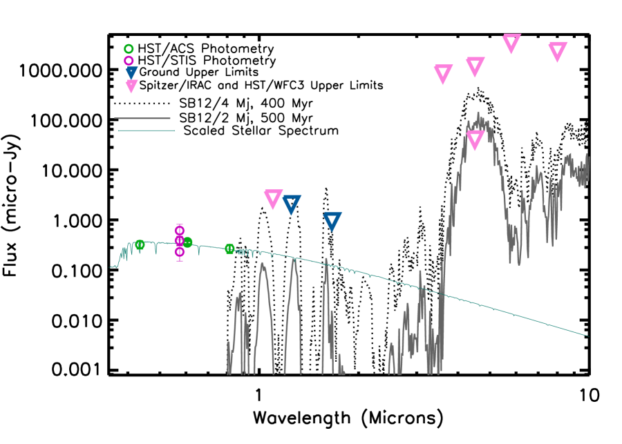
Figure 1: SED of Fomalhaut b (open circles and triangles) compared to a scaled-down version of the stellar spectrum and synthetic planet spectra (2–4 $M_{J}$, age = 400–500 $Myr$) from Spiegel & Burrows (2012). In addition to the data listed in Table 1, we plot the $STIS$ photometry from Kalas et al. (2013) (lower magenta circle) and Galicher et al. (2013) (upper magenta circle).

To assign a cross-sectional area and size to the dust emission in Fomalhaut b, we collect existing data for the spectral energy distribution (SED) and the spatial extent of the image. For the SED, we adopt published results from HST detections (Kalas et al., 2008; Currie et al., 2012; Galicher et al., 2013; Kalas et al., 2013) and from IR upper limits (Marengo et al., 2009; Janson et al., 2012; Currie et al., 2012, 2013). Figure 1 compares these data (Table 1) to predictions from model planet atmospheres and a scaled-down version of the stellar spectrum. In addition to data from Table 1, we include entries for $STIS$ photometry from Kalas et al. (2013) (bottom magenta circle), Galicher et al. (2013) (top magenta circle), and Currie et al. (2012) (middle magenta circle).

The IR non-detections at 1–5 $\rm\mu{\rm m}$ place strong constraints on thermal emission from a Jupiter-mass planet around a 200–400 Myr A-type star. The near-IR upper limits rule out planets more massive than $\sim$ 4–5 $M_{\rm J}$ (e.g., Currie et al., 2013). The $IRAC$ 4.5 $\rm\mu{\rm m}$ data allow masses less than 2 $M_{\rm J}$ (e.g., Janson et al., 2012; Currie et al., 2012).

The optical flux density measurements track a scaled down version of the Fomalhaut stellar photosphere (Currie et al., 2012). The three HST $ACS$ points in green closely follow the photosphere. At 0.6 $\rm\mu{\rm m}$, three independent reductions of $STIS$ photometry bracket the $ACS$ point. Given the errors, the three $STIS$ measurements agree reasonably well.

Together, the optical and IR data for Fomalhaut b strongly favor scattered light from dust over thermal emission from a Jupiter mass planet. In the optical, the flux is more than a factor of $100$ brighter than the emission expected from a planet and has the colors of an A-type star. In the IR, the upper limits on the flux density rule out planets more massive than 2 $M_{\rm J}$ and lie a factor of ten brighter than the emission expected from scattered light.

2.3 Spatial Extent of Fomalhaut b

Placing limits on the emitting area of Fomalhaut b requires an understanding of the HST point-spread-function (PSF) and the noise in $ACS$ and $STIS$. Several published results suggest the source is unresolved (Kalas et al., 2008; Currie et al., 2012). Others report the source is extended. Galicher et al. (2013) suggest the source is resolved in the F814W data; Kalas et al. (2013) attribute extended structure in the $STIS$ data to speckle noise.

To illustrate the difficulty in measuring the spatial scale of the dust in Fomalhaut b, we re-derive the PSF along the $x$ and $y$ axes of the F435W, F606W, and F814W reductions of $ACS$ data from Currie et al. (2012). We try two approaches. First, we construct radial intensity profiles in the $x$ and $y$ directions, re-sample the profile with a grid spacing of 0.25 pixels using linear interpolation, and measure the full-width-at-half-maximum (FWHM) using a minimum uncertainty of 1/2 a pixel ($\sim$ 13 mas). Second, we model the intensity profile as a 2D gaussian, using the mpfit package and adopt the average of results for the FWHM from a range of fit radii. Here, we include the standard deviation of these measurements in our uncertainty. For the highest-quality data (F606W), we derive the FWHM from both the the 2004 data and the 2006 data, averaging the results for two separate reductions of each data set.

Table 2 lists our results along with predictions for an unresolved point source. In the highest-quality data sets (2004 and 2006 F606W), Fomalhaut b is clearly consistent with a point source. At F435W, Fomalhaut b is slightly extended along the $y$ axis compared to a point source. However, this deviation is barely larger than 1-$\sigma$ and thus is not significant. The azimuthally-averaged FWHM (63 $\pm$ 20 mas; 65 $\pm$ 22 mas) is consistent with the point source.

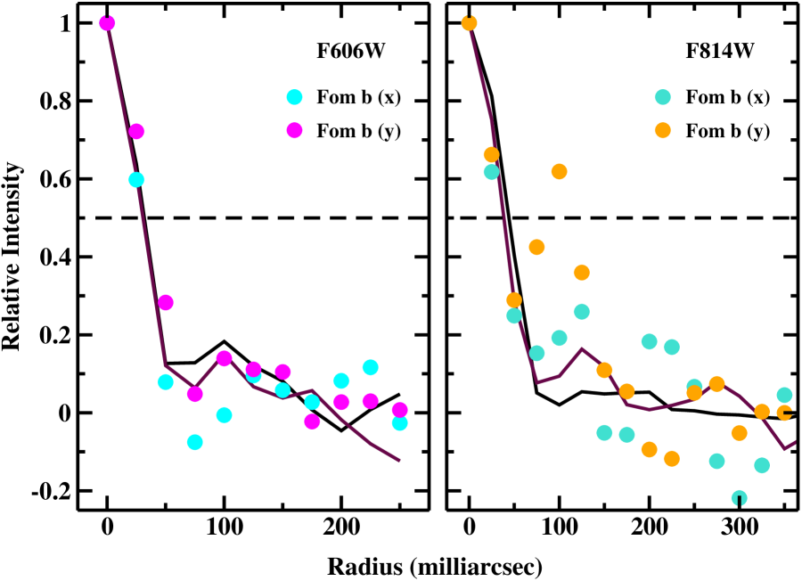
Figure 2: Normalized radial intensity profiles along the $x$ and $y$ axes for Fomalhaut b for F606W (left panel) and F814W (right panel). In each panel, black (maroon) lines indicate the intensity profile for a background star along the $x$ ($y$) axis. Fomalhaut b’s radial intensity profile at F606W is consistent with the point source. The profile at F814W is more difficult to interpret.

Figure 2 demonstrates the necessity of higher SNR data with well-sampled PSFs to assess the spatial extent of Fomalhaut b. In both panels, a background star (black and maroon lines) has a sharp core with FWHM $\approx$ 35 milliarcsec and a faint halo extending to roughly 200 milliarcsec. Within the errors, the $x$ and $y$ traces are indistinguishable. In F606W (left panel), the $x$ and $y$ traces of Fomalhaut b closely follow results for the point source. Although the F814W data (right panel) have a similarly sharp core inside 50 milliarcsec, both traces have much larger intensity than a point source at 100–200 milliarcsec. Based on this larger intensity, Galicher et al. (2013) conclude the source is extended. However, both traces also have several maxima, suggesting a significant noise component.

We conclude that Fomalhaut b is unresolved at F435W and at F606W. At F814W, current results are inconclusive due to the lower SNR relative to F606W. Adopting an angular diameter of 69 $\pm$ 14 milliarcsec from the highest SNR data (2006 F606W), an upper limit on Fomalhaut b’s projected radius is $R_{b}\lesssim R_{b,max}\approx$ 0.5 $\theta~{}D$ $\approx$ 0.27 $\pm$ 0.05 ($D$ / 7.7 pc) AU.

2.4 Limits on Emitting Area and Mass

Following the approach of Kalas et al. (2008), we estimate $A_{b}$ the cross-sectional area of dust in Fomalhaut b. The flux received from the star at the Earth is $f_{\star}=L_{\star}/4\pi D^{2}$. Fomalhaut b intercepts a fraction of the stellar flux $f_{b}=L_{\star}/4\pi r^{2}$, where $r$ = 120 AU. The observed flux from Fomalhaut b at Earth, $f_{o}=f_{b}A_{b}\ Q_{s}/4\pi D^{2}$, depends on the cross-sectional area $A_{b}$ and the scattering efficiency $Q_{s}$. Thus, $f_{o}$ = $(f_{\star}/4\pi r^{2})A_{b}\ Q_{s}$; $A_{b}=(4\pi r^{2}/Q_{s})(f_{o}/f_{\star})$.

Deriving $A_{b}$ requires three measured quantities, $r,f_{o},f_{\star}$, and one adopted quantity, $Q_{s}$. For the ratio $f_{o}/f_{\star}$, we define the contrast in optical magnitudes $\Delta m$ = -2.5 log ($f_{o}$/$f_{\star}$). Adopting $m$ = 1.2 for the primary and $m$ = 24.95 for Fomalhaut b, the cross-sectional area for $r\approx$ 120 AU is

$$A_{b}=1.3\times 10^{23}\left({0.1\over Q_{s}}\right)~{}{\rm cm^{2}}~{}.$$ (2)

This expression assumes grains with albedo similar to objects in the outer solar system ($Q_{s}\approx$ 0.1; Stansberry et al., 2008). Our estimate is midway between previous results of $A_{b}\approx 10^{23}(0.1/Q_{s})$ cm² (Kalas et al., 2008) and $A_{b}\approx 1.5\times 10^{23}(0.1/Q_{s})$ cm² (Galicher et al., 2013).

For simplicity, we adopt $A_{b}\approx 10^{23}$ cm². A spherical object with this $A_{b}$ has a radius, $R_{b}\gtrsim R_{b,min}\approx$ 10¹¹ cm $\approx$ 150 $R_{\oplus}$, somewhat larger than a solar radius and significantly larger than the radius of any planet.

If a dust cloud gravitationally bound to a planet produces the observed emission in Fomalhaut b, the size and emitting area constrain the mass of the planet (e.g., Kalas et al., 2008; Kennedy & Wyatt, 2011; Galicher et al., 2013; Kalas et al., 2013). For planets orbiting a star, material inside the Hill sphere is bound to the planet. The radius of the Hill sphere for a circular orbit is

$$R_{H}=a\left({M_{p}\over 3M_{\star}}\right)^{1/3}~{},$$ (3)

where $a$ is the semimajor axis of the planet. When planets have eccentric orbits, $R_{H}^{\prime}\approx(r/a)R_{H}$, where $r$ is the current distance from the planet to the star. With $r$ varying between $a(1-e)$ at periastron to $a(1+e)$ at apoastron, $R_{H}^{\prime}$ at periastron is $1-e$ smaller than $R_{H}$ (Hamilton & Burns, 1992). Setting $R_{b}$ equal to $R_{H}^{\prime}$, a rough limit on the mass of the planet is

$$M_{p}\approx 2\left({R_{b}\over 0.01~{}r}\right)^{3}~{}M_{\oplus}~{}.$$ (4)

The mass of the planet is very sensitive to $R_{b}$ (Kennedy & Wyatt, 2011; Kalas et al., 2013, and references therein). For a barely resolved Fomalhaut b with radius $R_{b}\approx R_{b,max}\approx$ 0.25 AU at $r\approx$ 35 AU, $M_{p}\approx$ 0.8 $M_{\oplus}$. If Fomalhaut b is optically thick, the minimum physical size of the cloud is roughly 0.01 AU. A strong lower limit on the mass of the planet is then roughly $10^{23}$ g (Kalas et al., 2008; Kennedy & Wyatt, 2011). Adopting $R_{b}\approx\gamma R_{H}^{\prime}$ with $\gamma\approx$ 0.2–0.3 (where orbits are definitely stable, e.g., Hamilton & Burns, 1992) to $\gamma\approx$ 2–3 (where some orbits are stable for long periods, e.g., Shen & Tremaine, 2008) leads to a much broader range of plausible planet masses (e.g., Kalas et al., 2008; Kennedy & Wyatt, 2011; Kalas et al., 2013).

2.5 Limits on Optical Depth

Previous studies of dust emission in Fomalhaut b focus on optically thin models (e.g., Kalas et al., 2008; Kennedy & Wyatt, 2011; Galicher et al., 2013; Kalas et al., 2013). A robust lower limit on the optical depth $\tau$ depends on the emitting area and the spatial extent. With $A_{b}$ $\approx$ $10^{23}$ cm² and $R_{b}\lesssim$ 0.25 AU, $\tau\approx A_{b}/\pi R_{b}^{2}$ $\gtrsim 2\times 10^{-3}$.

To derive an upper limit on $\tau$, we assume a cloud composed of particles with mass density $\rho$ and radius $R$. The swarm has radius $R_{b}\approx 10^{11}$ cm and total mass $M_{b}\approx A_{b}\rho R$. If the cloud is produced in a giant impact, the 8 yr baseline of the HST observations establishes a maximum expansion velocity of roughly 300 ${\rm cm~{}s^{-1}}$. Setting this velocity equal to the escape velocity of a colliding pair of icy planetesimals with mass density $\rho_{p}\approx$ 2 ${\rm g~{}cm^{-3}}$ yields a planetesimal radius $R_{p}\approx$ 5 km and mass $M_{p}\approx 5\times 10^{17}$ g. Requiring $M_{p}\approx M_{b}$ yields a typical particle size, $R\approx M_{p}/A_{b}\approx$ 0.05 $\rm\mu{\rm m}$. Even in an optically thick cloud, radiation pressure rapidly accelerates such small particles to velocities much larger than 300 ${\rm cm~{}s^{-1}}$ (e.g., Burns et al., 1979). Thus, an optically thick cloud from a giant impact cannot produce the observed scattered light emission from Fomalhaut b.

We now examine the possibility of an optically thick particle cloud orbiting a massive planet. Particles collide with a collision time $t_{c}$. In every collision, there is some dissipation of the collision energy. Over time, repeated dissipative collisions produce a flattened structure with a finite scale height set by the particle size and the semimajor axis of an orbit (e.g., Brahic, 1976). Collisions eject some particles from the system; others fall onto the planet. The optical depth declines.

The collision time for this process is $t_{c}\approx(n\sigma v)^{-1}$, where $n$ is the number density of particles, $\sigma$ is the cross-section, and $v$ is the relative velocity. For planets with mass $M_{p}\approx$ 0.1–10 $M_{\oplus}$, radiation pressure sets a minimum particle size $R\approx$ 100 $\rm\mu{\rm m}$ (e.g., Kennedy & Wyatt, 2011). The number density is $n\gtrsim 10^{-6}$ cm${}^{-3}(R/100~{}{\rm\mu{\rm m}})^{-2}$. Setting $v$ equal to the orbital velocity around the planet (e.g., Kennedy & Wyatt, 2011), the collision time depends only on the mass of the central planet:

$$t_{c}\lesssim 0.01\left({1~{}M_{\oplus}\ \over M_{p}}\right)^{1/2}~{}{\rm yr}~{}.$$ (5)

For any plausible planet mass, the collision time is 9–11 orders of magnitude smaller than the age of Fomalhaut. Thus, the optical depth of an optically thick cloud declines on time scales much shorter than the age of Fomalhaut.

Collision outcomes cannot change this conclusion. If collisions produce larger merged objects, the optical depth declines more rapidly. If collisions produce clouds of smaller particles, radiation pressure removes these particles on (i) the time scale for particles to orbit the planet, $t\approx$ 1 yr ($R\lesssim$ 5–10 $\rm\mu{\rm m}$) or (ii) the time scale for the planet to orbit the central star, $t\approx$ 1000 yr ($R\approx$ 10–100 $\rm\mu{\rm m}$). Both of these time scales are much shorter than the age of Fomalhaut.

This analysis suggests that Fomalhaut b is not a massive, optically thick cloud of small particles. For a cloud expanding from a giant impact, the particle size (0.05 $\rm\mu{\rm m}$) required for the derived mass is too small. If the cloud orbits a massive planet, the collision time is too short. Thus, we focus on optically thin models for the dust emission.

3 DUST MODELS

In giant impact models, two large protoplanets collide to produce an ensemble of objects with a broad range of sizes (e.g., Wyatt & Dent, 2002; Kenyon & Bromley, 2005). After the collision, the center-of-mass of the ensemble – which might contain a few massive objects – follows an orbit with angular momentum per unit mass comparable to the sum of the angular momenta of the two protoplanets. Other objects expand away from this orbit; smaller particles expand faster than larger particles. Although the initial expansion of the cloud is roughly spherical, orbital shear and collisions with other particles change the shape and the mass of the cloud on orbital time scales. After 10–20 orbital periods ($\sim 10^{4}$ yr for Fomalhaut b), the material lies in a narrow ring surrounding the central star.

Collisional cascades begin with a massive, roughly spherical (e.g., Bottke et al., 2010; Kennedy & Wyatt, 2011) or disk-shaped (Kalas et al., 2008) swarm of satellites orbiting a massive planet. Destructive collisions among the satellites produce copious amounts of debris (Bottke et al., 2010; Kennedy & Wyatt, 2011). Collisions within the debris yield even smaller particles. The resulting cascade of collisions slowly grinds small satellites into dust (e.g., Dohnanyi, 1969; Williams & Wetherill, 1994; Tanaka et al., 1996; O’Brien & Greenberg, 2003; Kobayashi & Tanaka, 2010). Radiation pressure and Poynting-Robertson drag remove small dust particles from circumplanetary orbits (Burns et al., 1979). Thus, the collisional cascade gradually removes material from the system. The time scale for the cascade is usually 10–100 Myr, much longer than the lifetime of material produced in a single, giant impact.

Continuous capture models combine aspects of both approaches (e.g., Ruskol, 1972; Weidenschilling, 2002; Estrada & Mosqueira, 2006; Koch & Hansen, 2011). In this picture, a massive planet lies embedded within a circumstellar disk. When circumstellar objects pass through the Hill sphere of the planet, they can lose energy through dynamical interactions with other objects outside the Hill sphere or through collisions with other objects inside the Hill sphere. If the energy loss is large enough, these objects become bound to the planet. Over time, high velocity collisions between the captured objects lead to the production of small dust grains. If collisions are fairly frequent and the net angular momentum of captured objects is large enough, collisional damping leads to the formation of a circumplanetary disk (Brahic, 1976). Otherwise, captured satellites lie in a roughly spherical cloud around the planet.

The evolution of solids within a captured cloud or disk depends on the accumulation rate. Here, we distinguish between the relatively rapid capture of a massive swarm of satellites during the early evolution of the planetary system (e.g., Nesvorný et al., 2007) from the slow capture of material throughout the evolution of the planetary system (e.g., Ruskol, 1972; Weidenschilling, 2002; Estrada & Mosqueira, 2006; Koch & Hansen, 2011). Prompt captures over a few Myr enable the immediate onset of a collisional cascade and formation of a massive dust cloud. Over time, this evolution may produce an irregular satellite system similar to those surrounding the giant planets of the solar system (e.g., Bottke et al., 2010; Kennedy & Wyatt, 2011). When captures occur intermittently, the mass in satellites grows slowly with time. As this mass grows, collisions gradually produce a cloud of debris. Thus, the time scale to produce an observable dust cloud is much longer. In less massive systems composed of small particles, some circumstances allow the particles to avoid collisions (e.g., Heng & Tremaine, 2010). For any outcome, the lifetime of the cloud or disk is 100 Myr or longer.

To isolate important issues in capture and cascade models, we examine two extreme cases. For cascades, we follow Kennedy & Wyatt (2011) and assume an initially massive cloud of satellites where destructive collisions and radiation pressure slowly reduce the mass with time. The ability of a cascade to match observations of Fomalhaut b then depends on the mass of the planet, the initial mass and size of the cloud, and the typical particle size (§3.4; see also Kennedy & Wyatt, 2011). For captures, we assume the initial mass of the cloud is zero and derive the capture rate for objects passing through the Hill sphere. Because the capture rate depends on the properties of the circumstellar disk and the planet (§3.3), the conditions required for successful capture models differ from those of cascade models. By focusing on the two models separately, we can place better limits on the source of material involved in either mechanism.

Aside from the lifetime, various observations might distinguish between these dust formation processes. Developing these constraints requires clear predictions for the mass, cross-sectional area, and other properties of the debris as a function of initial conditions and time. In the next sections, we derive basic properties of the debris expected from each model and compare our results with observations of Fomalhaut b. Our goal is to develop a better analytic understanding of each mechanism which will serve as the foundation for detailed numerical simulations in future studies.

3.1 Properties of the Debris

To establish the basic properties of a dusty cloud or disk of debris for Fomalhaut b, we consider an ensemble of solid particles with total mass $M_{d}$ and total cross-sectional area $A_{d}$. In most applications, the smallest particles have most of the area; the largest particles have most of the mass. Matching observations then requires (i) setting an appropriate size for the smallest particles, (ii) adopting a size distribution, and (iii) verifying that the largest particles contain a reasonable amount of mass. In this paper, our goal is to predict the range of particle sizes for specific theories of dust production and to learn whether these predictions match observations. With improved constraints, we develop a better understanding of the applicability and limitations of each theory.

To relate the area to the physical radii $R$ of the particles, we assume a size distribution $n(R)$, where the number of particles with radii between $R$ and $R+dR$ is a power law:

$$n(R)dR=n_{0}R^{-q}dR~{}.$$ (6)

The total number of particles between a minimum size $R_{min}$ and a maximum size $R_{max}$ is $N_{d}$.

Here, we require that the number of particles with $R\geq R_{max}$ is exactly 1. Integrating the size distribution from $R_{max}$ to infinity and adopting $q>1$:

$$n_{0}=(q-1)R_{max}^{q-1}~{}.$$ (7)

For typical $q\approx$ 3.5–6 (e.g., Dohnanyi, 1969; O’Brien & Greenberg, 2003; Kobayashi & Tanaka, 2010; Leinhardt & Stewart, 2012), it is very likely that the particle with $R\geq R_{max}$ has a radius $R_{max}$. Thus, we can integrate over the size distribution from $R_{min}$ to $R_{max}$ to derive the cross-sectional area:

$$A_{d}=\pi(q-1)R_{max}^{2}\left\{\begin{array}[]{lll}{\rm ln}(R_{max}/R_{min})&&q=3\\ \\ ((R_{max}/R_{min})^{q-3}-1)/(q-3){}&&q\neq 3\\ \end{array}\right.$$ (8)

For all $q>3$, the smallest particles contain most of the area. The total mass requires a similar integral:

$$M_{d}={4\pi\rho\over 3}(q-1)R_{max}^{3}\left\{\begin{array}[]{lll}{\rm ln}(R_{max}/R_{min})&&q=4\\ \\ ((R_{max}/R_{min})^{q-4}-1)/(q-4){}&&q\neq 4\\ \end{array}\right.$$ (9)

where $\rho$ is the mass density of the particles.

Our goal is to predict $A_{d}$ and $M_{d}$ for each model and to identify combinations of model parameters where the predictions match the observed $A_{b}$. Formally, we should augment $A_{d}$ and $M_{d}$ by the cross-sectional area and the mass of the single object with $R\geq R_{max}$. With a measured $A_{d}$ $\approx 10^{23}$ cm², the correction is less than one part in $10^{6}$ and safely ignored. For $q>4$, most of the mass is in the smallest objects; thus, the largest object makes a negligible contribution to $M_{d}$. For small $q\approx$ 3.5, a single object with $R=R_{max}$ adds roughly 1% to the mass. This correction is negligible.

In these expressions, $R_{max}$ sets the basic level for the mass and the area. The terms involving $R_{max}/R_{min}$ to the right of the left curly bracket then provide a scale factor. For $q\lesssim$ 4 and any $R_{max}/R_{min}$, the scale factor for the mass is negligible. For $q\gtrsim 4$ ($q\gtrsim$ 3), the scale factor for the mass (cross-sectional area) is very sensitive to $R_{max}/R_{min}$.

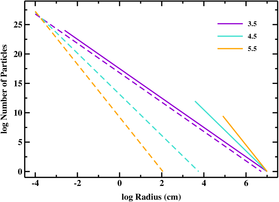
Figure 3: Size distributions for ensembles of particles with a total cross-sectional area $A_{d}=10^{20}$ cm². The legend indicates the slope $q$ of each size distribution. Solid curves: size distributions requiring $n(R\geq R_{max})=1$, with $R_{max}$ = 100 km. Dashed curves: size distributions requiring $R_{min}$ = 1 $\rm\mu{\rm m}$. Setting $R_{min}$ ($R_{max}$) yields ensembles with fewer (more) large particles and smaller (larger) total mass.

To specify the size distribution completely, we set $q$ and any two of $R_{min}$, $R_{max}$, or $A_{d}$. Fig. 3 shows an example where we adopt $A_{d}=10^{20}$ cm² and either $R_{min}$ = 1 $\rm\mu{\rm m}$ (dashed curves) or $R_{max}$ = 100 km (solid curves) for $q$ = 3.5, 4.5, or 5.5. When we fix $A_{d}$, $q$, and $R_{min}$, the maximum size $R_{max}$ and the total mass $M_{d}$ follow from eqs. (8–9). Fixing $A_{d}$, $q$, and $R_{max}$ establish different values for $R_{min}$ and $M_{d}$. For any $q$, there are an infinite number of combinations of $R_{min}$ and $R_{max}$ that yield identical area $A_{d}$. In general, setting a small value for $R_{min}$ (e.g., 1–10 $\rm\mu{\rm m}$) leads to smaller $R_{max}$ and $M_{d}$. Fixed $R_{min}$ also produces a small range in $N_{d}$ the total number of particles. Setting a large value for $R_{max}$ results in larger $R_{min}$ and $M_{d}$ and a smaller $N_{d}$.

Specifying the size distribution in terms of $M_{d}$ is more complicated. When $q<4$ and $R_{max}\gg R_{min}$, setting $q$ and $M_{d}$ establishes $R_{max}$ (eq. [9]). Fixing $R_{min}$ then yields $A_{d}$. For $q\geq 4$ (or when $R_{max}$ is not much larger than $R_{min}$ for any $q$), choosing any two of $R_{min}$, $R_{max}$, $A_{d}$, or $M_{d}$ then defines the remaining parameters. Although more cumbersome, this approach is an integral part of planet formation theory. We will return to it when we consider specific models for dust in the next sections.

The main parameters of the size distribution – $R_{min}$, $R_{max}$, and $q$ – depend on physical events throughout the planet formation process. In a collisional cascade, for example, the total mass in solids and the bulk properties of the solids establish $q$ and $R_{max}$ (e.g., O’Brien & Greenberg, 2003; Wyatt, 2008; Kenyon & Bromley, 2008; Krivov et al., 2008; Kobayashi & Tanaka, 2010; Belyaev & Rafikov, 2011). The luminosity of the central star sets $R_{min}$; radiation pressure ejects smaller particles on short time scales compared to the local orbital period and the lifetime of the cascade (Burns et al., 1979). In a giant impact, the kinetic energy and the bulk properties of the protoplanets set $R_{max}$, $q$, and the total mass of ejected material (e.g., Canup, 2004, 2005, 2011). These quantities establish $R_{min}$ uniquely (eq. [9]).

Within this framework, observations of the cross-sectional area of dust yield direct tests of planet formation theory. With the area known and $R_{min}$ derived from the stellar luminosity, choosing $q$ then yields a unique $R_{max}$. Similarly, choosing $R_{max}$ implies a unique $q$. Once $R_{min}$, $R_{max}$, and $q$ are known, comparisons with predictions from models of collisional cascades, giant impacts, or another mechanism provide clear tests of the theory.

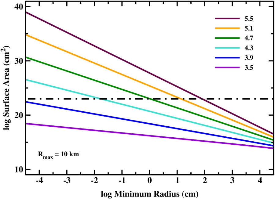
Figure 4: Relations between cross-sectional area and minimum radius for size distributions with $R_{max}$ = 10 km and various $q$ as indicated in the legend. For each size distribution, $N(R\geq R_{max})$ = 1. The dot-dashed line indicates $A_{d}$ = $10^{23}$ cm². At fixed $R_{min}$, size distributions with larger $R_{max}$ and smaller $q$ have smaller area.

To illustrate how these choices affect analyses of observations, we examine the variation of area with $R_{min}$ and $R_{max}$. In Fig. 4, we set $R_{max}$ = 10 km, require one object with $R\geq R_{max}$, and derive $A_{d}$ as a function of $R_{min}$ and $q$. The results behave as expected: ensembles of particles with larger $R_{min}$ have smaller area. With $R_{max}$ and $q$ fixed, the cross-sectional area grows as $R_{min}^{3-q}$. At fixed $q>3$, increasing $R_{min}$ reduces the area. Similarly, the area grows with $q$ at fixed $R_{min}$. As the size distribution becomes wider or steeper, the area grows.

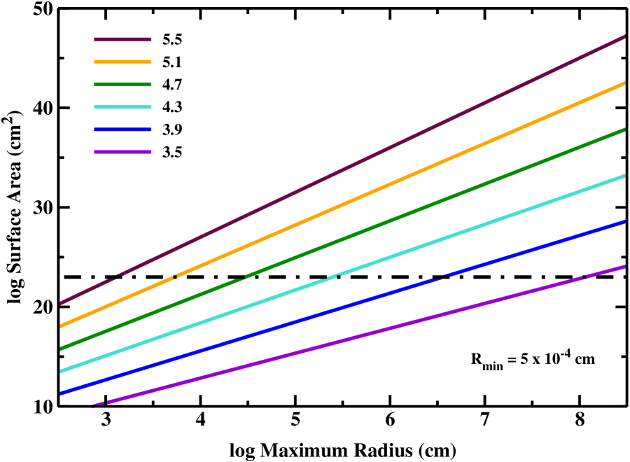
Figure 5: Relations between cross-sectional area and maximum radius for size distributions with $R_{min}$ = 5 $\rm\mu{\rm m}$ and various $q$ as indicated in the legend. For each size distribution, $N(R\geq R_{max})$ = 1. The dot-dashed line indicates $A_{d}$ = $10^{23}$ cm². At fixed $R_{max}$, size distributions with larger $R_{max}$ and larger $q$ have larger area.

With $R_{min}$ fixed, the area is also sensitive to $R_{max}$ (Fig. 5). Here, we set $R_{min}$ = 5 $\rm\mu{\rm m}$, require one object with $R\geq R_{max}$, and derive $A_{d}$ as a function of $R_{max}$ and $q$. At fixed $R_{max}$, the area scales with $R_{max}^{q-1}$ (eqs. [1–2]). Thus, size distributions with larger $q$ have much larger area than those with smaller $q$. Extending the size distribution to larger and larger $R_{max}$ yields larger $A_{d}$ for all $q$. Although this result is somewhat counterintuitive, it is a consequence of our requirement of one object with $R\geq R_{max}$. The area grows with the number of very small objects, which grows as $R_{max}^{q-1}$. Thus, for any $q>1$, size distributions with larger $R_{max}$ have much larger area.

For Fomalhaut b, these results place interesting constraints on models for dust emission. The data reviewed in §2 suggest an optically thin cloud with $A_{b}$ $\approx 10^{23}$ cm² and $R_{min}$ $\approx$ 5 $\rm\mu{\rm m}$. Fig. 4 rules out size distributions with $R_{max}$ = 10 km and either $q\lesssim$ 3.9 or $q\gtrsim$ 4.1. From Fig. 5, larger (smaller) $R_{max}$ yields more (less) area. Thus, optically thin models with $q\lesssim$ 3.9 can match the observed area with larger $R_{max}$. Similarly, optically thin models with $q\gtrsim$ 4.1 can match observations with smaller $R_{max}$.

Assuming Fomalhaut b has dust particles as small as 5–10 $\rm\mu{\rm m}$, Fig. 5 establishes combinations of $q$ and $R_{max}$ that match the observed area. The implied range in $R_{max}$ is enormous: from $R_{max}\approx$ 10 m for $q$ = 5.5 to $R_{max}$ $\approx$ 1 km for $q$ = 4.5 to $R_{max}$ $\approx$ 1000 km for $q$ = 3.5. From Fig. 3, each of these prescriptions to achieve the target $A_{d}$ will have very different total masses.

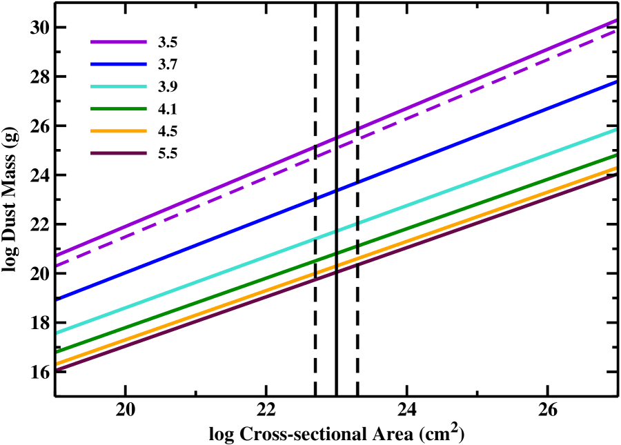
Figure 6: Relations between dust mass and cross-sectional area for power-law size distributions (eq. [6]), with $R_{min}$ = 5 $\rm\mu{\rm m}$, a range of $R_{max}$ (as in Fig. 5), and the range of $q$ indicated in the legend. The dashed curve repeats results for $R_{min}$ = 1 $\rm\mu{\rm m}$. Vertical lines: inferred cross-sectional area for a dust cloud in Fomalhaut b (solid line) with factor of two uncertainty (dashed lines). For fixed $A_{d}$, steeper size distributions (with larger $q$) require less total mass in dust.

To establish limits on the total dust mass, Fig. 6 plots $M_{d}$ as a function of $A_{d}$ for $R_{min}$ = 5 $\rm\mu{\rm m}$ and various $R_{max}$ and $q$. For fixed $A_{d}$, ensembles of dust with steeper size distributions (large $q$) require much less dust mass than ensembles with shallower size distributions (small $q$). For fixed $q$, larger areas require larger masses. With $n_{0}\propto R_{max}^{q-1}$, the range in dust mass at small $A_{d}$ is roughly two orders of magnitude smaller than at large $A_{d}$. In Fomalhaut b, the range of likely dust masses is somewhat more than 5 orders of magnitude ($M_{d}$ = $10^{20}$ g for $q$ = 5.5 to $M_{d}$ = $2\times 10^{25}$ g for $q$ = 3.5).

To provide better constraints on the properties of the dust size distribution, we now consider plausible origins for the solid material in Fomalhaut b. After deriving constraints for dust produced in a giant impact, we explore the structure of a circumplanetary disk composed of (i) debris captured from the protoplanetary disk and (ii) debris from collisions of satellites orbiting the planet.

3.2 Impact Models

Giant impacts generally have two possible outcomes (i) an expanding, isolated dust cloud orbiting the central star (e.g., Kenyon & Bromley, 2005; Galicher et al., 2013) or (ii) a disk or cloud of debris surrounding a (binary) planet (e.g., Asphaug et al., 2006; Canup, 2011; Leinhardt & Stewart, 2012). The large area of the dust cloud in Fomalhaut b probably eliminates the second option. At the distance of Fomalhaut b from Fomalhaut, likely giant impacts involve Earth-mass or smaller planets (Kenyon & Bromley, 2008, 2010). Detailed SPH simulations (e.g., Canup, 2011) suggest most of the debris orbits the planet at less than 10–30 times the radius of the planet. Although tidal forces can expand the orbits of debris particles (Kenyon & Bromley, 2014), the likely outer radius of the debris is still a factor of five to ten smaller than the minimum radius for a cloud in Fomalhaut b, $R_{c}\approx$ 300 $R_{\oplus}$ (§2; see also Tamayo, 2013). Thus, we explore models of debris within an isolated dust cloud.

3.2.1 Ejected Mass

We consider a simple head-on collision of two protoplanets with radii $R_{1},R_{2}$, mass $M_{1},M_{2}$, mass density $\rho_{p}$, and collision velocity $v_{c}$. Defining $M_{esc}$ as the mass ejected from the event, the largest remnant has a mass $M_{LR}$ = $M_{1}+M_{2}-M_{esc}$. If all the debris resides in a single object, $M_{esc}=4\pi\rho_{p}R_{esc}^{3}/3$. The size of the largest object in the debris – often called the largest fragment or the second largest remnant – has $R_{LF}\ =f_{LF}R_{esc}$ with $f_{LF}\approx$ 0.1–0.8. Thus, the mass of the largest fragment has a typical mass $M_{LF}=f_{LF}^{3}M_{esc}$ $\approx 10^{-3}-0.5~{}M_{esc}$ (see Benz & Asphaug, 1999; Durda et al., 2004; Giacomuzzo et al., 2007; Leinhardt & Stewart, 2012, and references therein).

To estimate $M_{esc}$, we consider two prescriptions for high speed collisions in a protoplanetary disk. When $M_{2}\ll M_{1}$, the impact produces a crater and ejects material from the surface of the larger protoplanet. The ejecta have a power law distribution of velocities, with $f(v>v_{c})\propto(v/v_{c})^{-\alpha}$ and $\alpha\approx$ 1–3 (e.g., Gault et al., 1963; Stoeffler et al., 1975; O’Keefe & Ahrens, 1985; Housen & Holsapple, 2003, 2011, and references therein). Although it is possible to derive the ejected mass from theoretical expressions for the kinetic energy of the impact and the binding energy of the larger protoplanet (e.g., Davis et al., 1985; Leinhardt & Stewart, 2012, and references therein), Housen & Holsapple (2011) derive the ratio $M_{esc}$/$M_{2}$ from a variety of laboratory measurements of point-mass projectiles impacting much larger targets. Extrapolating the results in their Fig. 16 suggests $M_{esc}/M_{2}\approx f_{cr}(v_{c}/v_{esc})^{\alpha}$, where $f_{cr}\approx$ 0.01 and $\alpha\approx$ 1.0–1.5 (for a recent application of this approach to asteroids in the Solar System, see Jewitt, 2012). For comparison, Svetsov (2011) derives $f_{cr}\approx$ 0.03 and $\alpha\approx$ 2.3 from a suite of theoretical calculations of cratering impacts (e.g., Greenberg et al., 1978).

To derive a simple expression for $M_{esc}$, we adopt $\alpha$ = 1.5 and a mass density $\rho_{p}=1.5$ g cm^-3. Setting $v_{esc}$ as the escape velocity of the larger protoplanet (e.g., Jewitt, 2012; Galicher et al., 2013):

$${M_{esc}\over M_{2}}\approx 3.7\times 10^{4}f_{cr}v_{c}^{1.5}~{}R_{1}^{-1.5}~{}.$$ (10)

Larger impact velocities produce more debris. Impacts onto more massive protoplanets yield less debris.

For high velocity collisions between objects with roughly equal masses, results for cratering impacts provide a less accurate measure of the ejected mass (e.g., Davis et al., 1985; Benz & Asphaug, 1999; Asphaug et al., 2006; Leinhardt & Stewart, 2009, 2012). Recent numerical simulations establish collision outcomes over a broad range in $M_{2}/M_{1}$. The ejected mass is fairly well-represented by a simple expression,

$${M_{esc}\over M_{tot}}\approx 0.5\left({Q_{c}\over Q_{d}^{*}}\right)^{\beta}~{}.$$ (11)

Here, $Q_{c}$ is the center-of-mass collision energy per unit mass, $Q_{d}^{*}$ is the collision energy per unit mass required to disperse 50% of the total mass $M_{tot}=M_{1}+M_{2}$ to infinity, and $\beta\approx$ 1–1.25. The $Q_{d}^{*}$ term is roughly equivalent to the binding energy per unit mass and depends on the physical properties of the protoplanets:

$$Q_{d}^{*}=Q_{b}R^{\epsilon_{b}}+Q_{g}\rho_{p}R^{\epsilon_{g}}~{}.$$ (12)

In this expression, $R$ is the radius of a protoplanet with mass $M_{tot}$, $Q_{b}R^{\epsilon_{b}}$ is the bulk component of the binding energy and $Q_{g}\rho_{g}R^{\epsilon_{g}}$ is the gravity component of the binding energy. For most materials (e.g., Benz & Asphaug, 1999; Leinhardt & Stewart, 2012), the bulk (gravity) component of the binding energy dominates for solid objects with $R\lesssim$ 0.01 km ($R\gtrsim$ 0.01 km).

Here, we concentrate on catastrophic collisions of large objects in the gravity regime. For reduced mass $\mu=M_{1}M_{2}/(M_{1}+M_{2})$, $Q_{c}=0.5\mu v_{c}^{2}/(M_{1}+M_{2})$. To compare with eq. (10), we adopt $M_{2}\ll M_{1}$. The center of mass collision energy is then $Q_{c}\approx 0.5(M_{2}/M_{1})v_{c}^{2}$. For icy objects with $\rho_{p}=1.5$ g cm^-3, the binding energy parameters are $Q_{g}\approx 0.2$ and $\epsilon_{g}\approx 1.3$ (e.g., Benz & Asphaug, 1999; Leinhardt et al., 2008; Leinhardt & Stewart, 2009). With $\beta\approx$ 1 (Leinhardt & Stewart, 2012), the mass in debris is

$${M_{esc}\over M_{2}}\approx f_{cat,1}v_{c}^{2}R^{-1.3}~{},$$ (13)

where $f_{cat,1}\approx$ 0.83.

For equal mass protoplanets with $M_{1}\approx M_{2}$, collisions have a center-of-mass collision energy $Q_{c}=v_{c}^{2}/8$. Setting $R\approx\sqrt[3]{2}R_{1}$ for the radius of a merged object with $M_{tot}=M_{1}+M_{2}\approx 2M_{1}\approx 2M_{2}$, the ejected mass is:

$${M_{esc}\over M_{2}}\approx f_{cat,2}~{}v_{c}^{2}~{}R_{1}^{-1.3}~{},$$ (14)

with $f_{cat,2}\approx 0.31$. Compared to collisions with $M_{2}\ll M_{1}$, $Q_{c}$ is much smaller when $M_{1}\approx M_{2}$. Thus, $f_{cat,2}$ is much smaller than $f_{cat,1}$.

To derive results for the ejected mass, we specify the collision velocity. For two protoplanets on intersecting orbits around the central star, $v_{c}^{2}=v_{0}^{2}+v_{esc}^{2}$, where $v_{0}$ is the relative velocity of the two protoplanets at infinity. Small protoplanets have negligible self-gravity; the collision velocity is then the relative velocity. For large protoplanets with significant self-gravity ($R\gtrsim$ 10–100 km), the collision velocity is roughly the escape velocity.

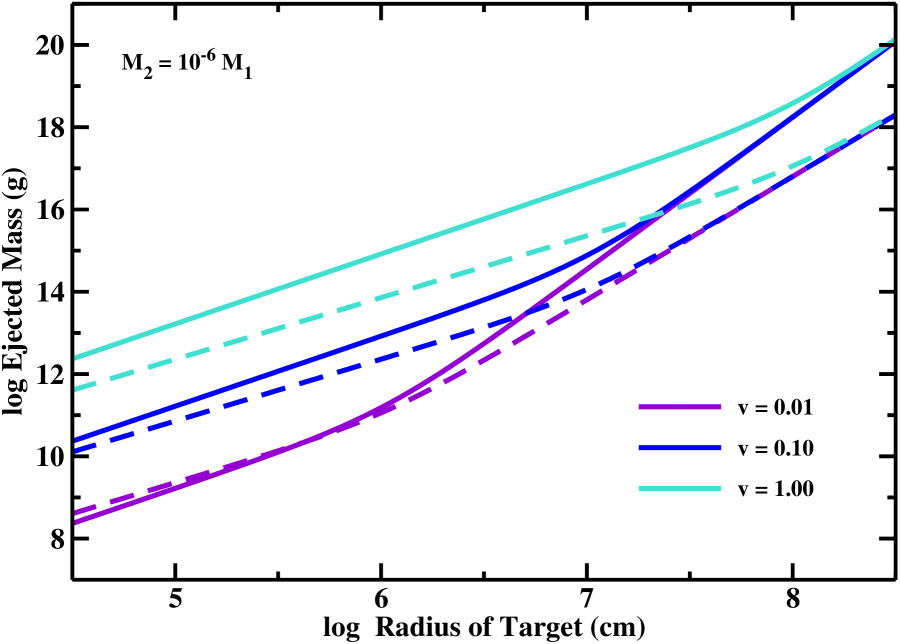
Figure 7: Relation between $M_{esc}$ and $R_{1}$ for collisions with $M_{2}=10^{-6}M_{1}$ and various collision velocities in ${\rm km~{}s^{-1}}$. Solid curves: results using eq. (13). Dashed curves: results using eq. (10). In either approach, ejecting the minimum dust mass required in Fomalhaut b requires very high velocity collisions onto massive objects with $R_{1}\gtrsim$ 1000 km.

Fig. 7 shows relations between $M_{esc}$ and the radius of the target protoplanet for collisions with $M_{2}=10^{-6}M_{1}$ and several collision velocities. Low velocity impacts ($v_{0}\approx$ 0.01-0.10 ${\rm km~{}s^{-1}}$) on low-mass targets ($R\approx$ 1–10 km) yield little dust, $M_{esc}$ $\approx 10^{10}-10^{12}$ g. In this regime, the self-gravity of the larger protoplanet is negligible; $M_{esc}$ depends only on $v_{0}$. The two expressions for collisions with low mass projectiles then yield similar amounts of debris.

As the impact velocity and target radius grow, the self-gravity of the protoplanet becomes more and more important. The ejected mass is then independent of $v_{0}$ and depends on the escape velocity of the larger protoplanet. In this regime, the expression derived for cratering impacts (eq. [10]) yields much smaller amounts of ejected mass than results derived from fits to numerical simulations (eq. [11]). Because their structure contains more flaws, larger objects are relatively easier to break than smaller objects (Benz & Asphaug, 1999; Housen & Holsapple, 2003). In higher velocity collisions, more of the target is involved in the collision. Higher velocity collisions onto larger targets then eject more material per unit collision energy. Fits to numerical simulations (eq. [11]) capture this complexity more accurately than estimates derived from the escape velocity (eq. [10]). Thus, the numerical results provide more accurate estimates for the ejected mass than the analytic expression.

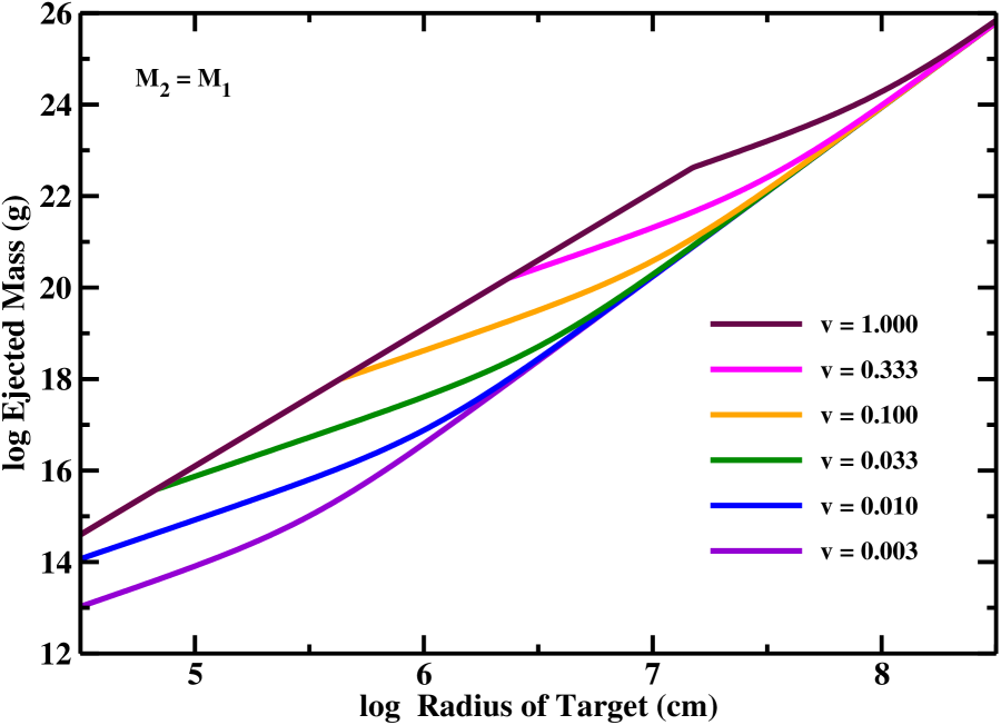
Figure 8: Relation between $M_{esc}$ and $R_{1}$ for collisions with $M_{2}=M_{1}$ and various collision velocities in ${\rm km~{}s^{-1}}$. Ejecting the broad range of plausible dust masses in Fomalhaut b requires moderate to high velocity collisions between objects with radii of 10–1000 km.

Fig. 8 shows the relation between $M_{esc}$ and radius for equal mass protoplanets. When protoplanets are small, $R\lesssim$ 1–3 km, the highest velocity collisions completely disrupt the target. The ejected mass is then the sum of the two protoplanet masses, setting the upper left edge of the curves in Fig. 8. For larger protoplanets, the escape velocity sets a lower limit on the impact velocity. This lower limit establishes the lower right edge of the curves. As a result, the range of ejected masses is fairly small – roughly two orders of magnitude – for any target radius. Although larger protoplanets are less prone to complete disruption, collisions between Earth-mass protoplanets still eject several lunar masses of material (e.g., Canup & Asphaug, 2001; Canup, 2004).

3.2.2 Surface Area

To derive the total cross-sectional area of fragments $A_{d}$ from the ejected mass $M_{esc}$, we must specify the parameters of the size distribution. In laboratory experiments and theoretical simulations, $q$, $R_{min}$, and $R_{max}$ depend on the parameters of the experiment or the simulation (e.g., Housen & Holsapple, 2011; Leinhardt & Stewart, 2012). However, many of these quantities cannot be inferred from observations. Thus, we fix $q$ and derive $R_{min}$ and $R_{max}$. Setting $q<4$ establishes the maximum radius, $R_{max}\ \approx(3(q-1)M_{esc}/4\pi\rho)^{1/3}$ (eq. [9]). This approach yields a largest fragment with $f_{LF}$ = $R_{max}$/$R_{esc}$ $\approx$ 0.6, which is close to the sizes of the largest fragments observed in laboratory experiments or numerical simulations (Benz & Asphaug, 1999; Leinhardt & Stewart, 2012). The minimum radius is formally arbitrary; for practical applications, stellar radiation pressure defines $R_{min}$.

When $q>4$ and $R_{max}\ \gg$ 1 cm, the first term in eq. (9) dominates. To make progress, we consider a range of $f_{LF}$ = $R_{max}$/$R_{esc}$ $\approx$ 0.01–0.6 which more than covers the typical range, $f_{LF}$ $\approx$ 0.1–0.6, in experiments and simulations. Once $f_{LF}$ and $R_{max}$ are known, eq. (9) yields $R_{min}$.

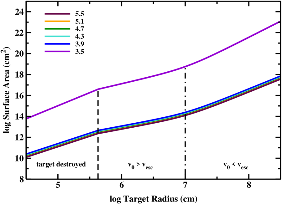
Figure 9: Surface area of ejecta as a function of the radius of the target for collisions between equal mass targets with $v_{0}$ = 0.1 ${\rm km~{}s^{-1}}$, $f_{LR}$ = 0.6, and various $q$ as listed in the legend. For large $f_{LR}$, most of the mass is in the largest fragment. When the slope of the size distribution is relatively shallow ($q\approx$ 3.5), the fragments extend to small sizes which have large surface area per unit mass. When the slope is steep, the ensemble of particles has fewer low mass fragments and smaller surface area.

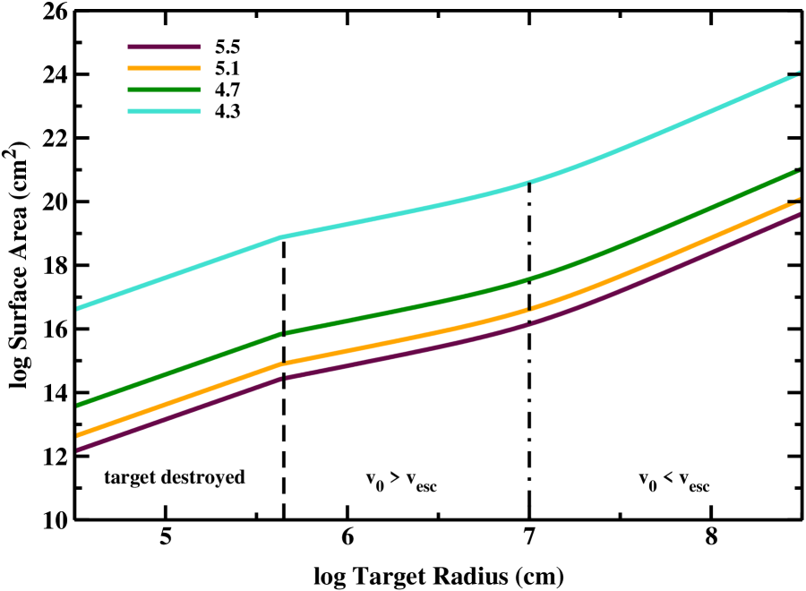
Figure 10: As in Fig. 9 for $f_{LR}$ = 0.1. Placing less mass in the largest fragment leaves more mass for smaller fragments. Thus, smaller $f_{LR}$ produces ensembles of dust with larger surface area per unit mass.

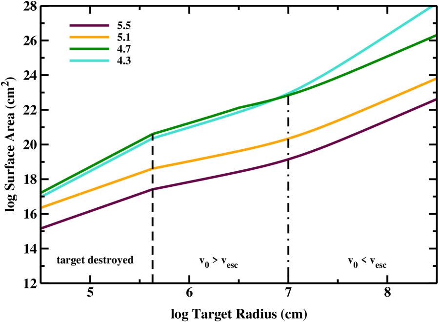
Figure 11: As in Fig. 9 for $f_{LR}$ = 0.01.

Figs. 9–11 illustrates the variation of the area with target radius for collisions between equal mass targets with $v_{0}$ = 0.1 ${\rm km~{}s^{-1}}$, various $q$, and $f_{LF}$ = 0.6 (Fig. 9), $f_{LF}$ = 0.1 (Fig. 10), and $f_{LF}$ = 0.01 (Fig. 11). For $q$ = 3.5 and 3.9, requiring one object with a radius of $R_{max}$ establishes $f_{LF}$ = 0.6; thus, only Fig. 9 shows results for these values of $q$.

For each value of $q$ (indicated by the legend), the relation between the cross-sectional area and target radius has three regimes. Small protoplanets with $R\lesssim$ 5 km are the weakest and the easiest to break. In collisions with modest velocities, the projectile and the target are completely destroyed. The area of the ejected material then increases with target radius as $A_{d}\propto R^{2.5}$. For somewhat larger protoplanets (indicated by the vertical dashed line in each Figure), the binding energy per unit mass grows slowly ($\propto R^{1.3}$) compared to an ideal monolithic object ($\propto R^{2}$). Modest velocity impacts do not destroy these protoplanets. When $v_{0}\gtrsim v_{esc}$, the area of the ejecta grows slowly with increasing radius, $A_{d}\propto R^{1.5}$. Among the largest protoplanets, where $v_{0}\lesssim v_{esc}$, collisions occur at the escape velocity. The collision energy then scales with $v_{esc}^{2}\propto R^{2}$, which grows much faster with radius than the binding energy ($\propto R^{1.3}$). The area then grows roughly with the volume of the protoplanets, $A_{d}\propto R^{3}$.

The variation of cross-sectional area with $q$ has a different topology in each Figure. When $f_{LF}$ = 0.6 (Fig. 9), roughly 20% of the ejected mass lies in the largest fragment. For steep size distributions with $q\gtrsim$ 3.9, the number of smaller particles increases very rapidly with radius; $R_{min}$ is always large, roughly a few meters to several tens of meters. The ratio of the area to the mass is then small. Thus, ensembles of particles with $f_{LF}$ = 0.6 and $q\gtrsim$ 3.9 have small area. For more shallow size distributions with $q\approx$ 3.5, the size distribution extends to much smaller radii, $R_{min}$ $\approx$ 1 $\rm\mu{\rm m}$. These ensembles have much larger area.

When $f_{LF}$ = 0.1 (Fig. 10), ensembles with $q\gtrsim$ 3.9 have much larger area. As $f_{LF}$ declines, the largest fragment has a smaller and smaller fraction of the total mass. With more mass available for smaller objects, the size distribution extends to smaller $R_{min}$. Ensembles of particles with smaller $R_{min}$ have larger area (eq. [8]).

This trend continues for $f_{LF}$ = 0.01 (Fig. 11). When the largest fragment has only 0.0001% of the total ejected mass, the size distribution can extend to the smallest allowed sizes ($R_{min}$ = 5 $\rm\mu{\rm m}$ for Fomalhaut). For $q\approx$ 4.3–4.7, the cross-sectional area saturates for target radii smaller than roughly 100 km. For larger $q$, $R_{min}$ is much larger than 5 $\rm\mu{\rm m}$; the area per unit ejected mass then remains fairly small.

For the observed cross-sectional area of roughly $10^{23}$ cm² in Fomalhaut b, these results provide clear constraints on plausible protoplanets involved in a single giant impact. Adopting the $f_{LF}$ $\approx$ 0.1–0.6 derived from numerous theoretical simulations sets a firm upper limit on the radius of the target, $R\lesssim$ 1000–2000 km. Extending the plausible range of fragment sizes to $f_{LF}$ $\approx$ 0.01 allows collisions among smaller targets, $R\sim$ 100 km, providing $q\approx$ 4.3–4.7.

3.2.3 Summary

Using only collision dynamics and the properties of power-law size distributions, we generate several useful expressions for the mass ejected during a collision of two high velocity objects. In all collisions, the ejected mass depends on the escape velocity and the relative velocity of the impactors. When the mass ratio between the impactors is large (Fig. 7), large ejected masses require high velocity collisions onto very massive protoplanets. When the mass ratio is near unity, somewhat less energetic collisions yield comparable amounts of ejected material (Fig. 8). For the relative velocity expected during the late stages of planet formation, the range in the ejected mass is 2–3 orders of magnitude (Fig. 8). Coupled with our expressions for the area (eq. [8]) and mass (eq. [9]), these results yield the cross-sectional area as functions of the radii of the impactors and the fraction of mass $f_{LF}$ in the largest fragment of the debris (Figs. 9–11). For $f_{LF}$ = 0.6, ensembles of particles with $q\gtrsim$ 3.9 have little area per unit mass. As $f_{LF}$ in the ejecta decreases, particles with steeper size distributions have larger area.

Applying this analysis to Fomalhaut b strongly favors impacts between roughly equal mass protoplanets. For ensembles of particles in an extended dust cloud containing one large object with $R=R_{max}$ and no small objects with $R\lesssim R_{min}$ = 5 $\rm\mu{\rm m}$, we set limits on $R_{max}$ and the total mass $M_{d}$ as functions of $q$. Our results indicate $R_{max}\approx$ 10 m and $M_{d}$ $\approx 10^{20}$ g for $q$ = 5.5, $R_{max}\approx$ 1 km and $M_{d}$ $\approx 10^{20}$ g for $q$ = 4.5, $R_{max}\approx$ 30 km and $M_{d}$ $\approx 2\times 10^{23}$ g for $q$ = 3.9, and $R_{max}\approx$ 1000 km and $M_{d}$ $\approx 3\times 10^{25}$ g for $q$ = 3.5.

Quantitative models for the ejected mass as a function of the collision energy place additional limits on the giant impact picture. Standard results for the radius of the largest fragment in a high velocity collision suggest target radii of 1000–2000 km. If laboratory experiments and numerical simulations overestimate the typical size of the largest fragment by a factor of ten, collisions between two 100 km protoplanets produce enough dust when $q\approx$ 4.3–4.7.

These results limit the practicality of giant impact models for dust in Fomalhaut b (e.g., Kenyon & Bromley, 2005). When $f_{LF}\gtrsim$ 0.1, the required impactors are very large with radii of 1000–2000 km. Collisions between such large objects are very rare. For the surface density at 30–130 AU outlined in §2.1 (eq. [1]), a lower limit on the collision rate for two 1000 km objects within a 10 AU annulus is 1 per 50–100 Myr (Kenyon & Bromley, 2008, Appendix). With a typical cloud lifetime of a few orbits or less (Kenyon & Bromley, 2005), detecting dust from this collision is very unlikely.

Allowing $f_{LF}\approx$ 0.01 allows smaller targets with radii of 100 km. Collisions between two 100 km objects within a 10 AU annulus centered at 120 AU are fairly common, with a lower limit of roughly once every $5\times 10^{3}-10^{4}$ yr. Although numerical simulations of collisions between pairs of 100 km particles often yield debris with $q\approx$ 4.5 (Leinhardt & Stewart, 2012), outcomes with $f_{LF}\approx$ 0.01 are rare. Despite the modest frequency, collisions which yield such small fragments seem unlikely.

3.3 Continuous Capture into a Circumplanetary Cloud

Originally envisioned as an explanation for the origin of the Moon (Ruskol, 1961), the capture of circumstellar material onto circumplanetary orbits provides an interesting alternative to dust formation from a giant impact (for an application to satellite formation around Jupiter, see Estrada & Mosqueira, 2006; Koch & Hansen, 2011). In the simplest form of this model, an object enters the Hill sphere of a planet and collides with another object passing through the Hill sphere (Ruskol, 1972), a satellite of the planet (Durda & Stern, 2000; Stern, 2009), or the planet (Wyatt & Dent, 2002; Kennedy & Wyatt, 2011). Close approaches between a low-mass binary and a planet (Agnor & Hamilton, 2006, and references therein) or two planets (Nesvorný et al., 2007) often yield a bound satellite. Sometimes dynamical interactions with objects outside the Hill sphere produce a bound satellite (Ruskol, 1972; Goldreich et al., 2002). In a variant of this mechanism, objects find temporary orbits around the planet and become bound after collisions with other small objects or dynamical interactions with other planets (Kortenkamp, 2005; Suetsugu et al., 2011; Pires dos Santos et al., 2012; Suetsugu & Ohtsuki, 2013).

3.3.1 Captured Mass

To make an initial exploration of this picture for the formation of dust clouds surrounding an exoplanet, we estimate the capture rate from collisions of two circumstellar objects within the Hill sphere of a planet. In this mechanism, material enters the Hill sphere at a rate $\dot{M}_{H}$. The probability of a collision in the Hill sphere is the optical depth $\tau_{c}$ of the circumstellar disk in the vicinity of the planet. After the collision, the planet captures a fraction $f_{cap}$ of the material into bound orbits. The capture rate is then $\dot{M}_{cap}\approx\dot{M}_{H}\tau_{c}f_{cap}$.

The rate $\dot{M}_{H}$ depends on $\Sigma$ the local surface density of material, $\sigma$ the cross-section of the Hill sphere, and $\Omega$ the local angular frequency of the planet’s orbit (e.g., Lissauer, 1987; Goldreich et al., 2004). For objects with a modest amount of gravitational focusing, $\dot{M}_{H}\approx 3\Sigma\sigma\Omega$. We adopt a power-law surface density with the parameters from §2.1. For a planet with mass $M_{p}$ around a star of mass $M_{\star}$, the cross-section of the Hill sphere is $\pi R_{H}^{2}$. Material outside $a\gtrsim\gamma R_{H}$ with $\gamma\approx$ 0.3–0.4 is unbound (e.g., Hamilton & Burns, 1992; Hamilton & Krivov, 1997; Toth, 1999; Shen & Tremaine, 2008; Martin & Lubow, 2011). Thus, $\sigma\approx\pi\gamma^{2}R_{H}^{2}$.

The optical depth depends on the size distribution of circumstellar objects. During the late stages of the planet formation process, large objects contain nearly all of the mass and have a roughly power-law size distribution (e.g., Wetherill & Stewart, 1989; Kobayashi & Tanaka, 2010; Kenyon & Bromley, 2012). To set plausible limits on the optical depth in this regime, we consider two approaches. To establish a reasonable lower limit on the optical depth, we adopt a mono-disperse set of objects with radius $R_{max,d}$ and mass density $\rho_{d}$ = 1 ${\rm g~{}cm^{-3}}$; then $\tau_{c,m}\approx 3\Sigma/4R_{max,d}$. For a reasonable upper limit, a size distribution (eq. [6]) with $R_{min}$ = 1 km and $q\approx$ 4 yields $\tau_{c,sd}\approx 20\tau_{c,m}$. We set $R_{max,d}$ = 100 km for both limits.

At 100 AU, the typical optical depth is small. With $R_{max,d}$ = 100 km and $\Sigma\approx$ 0.3 ${\rm g~{}cm^{-2}}$, $\tau_{c,m}\approx 3\times 10^{-8}$. To match the observed lower limit of $\tau_{b}\gtrsim 10^{-3}$, planets must capture at least $10^{5}$ times the amount of material passing through their Hill spheres.

The fraction of colliding material captured by the planet depends on the relative velocities of planetesimals and the escape velocity of the planet (e.g., Ruskol, 1972; Weidenschilling, 2002). For material at 0.2–0.3 $R_{H}$, $f_{cap}\approx 1-3\times 10^{-3}$. Thus, the planet captures less than 1% of material colliding within its Hill sphere.

Combining $\dot{M}_{H}$, the two limits for $\tau$, and $f_{cap}$, the total capture rate is

$$\dot{M}_{cap} \approx 4.25-85~{}\times~{}10^{13}\left({f_{cap}\over 2\times 10^{-3}}\right)\left({d\over 1.0}\right)^{2}\left({\gamma\over 0.3}\right)^{2}\left({\Sigma_{0}\over{\rm 30~{}g~{}cm^{-2}}}\right)^{2}\left({M_{p}\over M_{\oplus}}\right)^{2/3}$$

$$~{}~{}~{}~{}~{}~{}~{}~{}~{}~{}~{}~{}~{}~{}~{}~{}~{}~{}~{}~{}~{}~{}\left({r\over{\rm 120~{}AU}}\right)^{-3/2}\left({M_{\star}\over 2~{}M_{\odot}}\right)^{11/6}\left({R_{max,d}\over{\rm 100~{}km}}\right)^{-1}~{}{\rm g~{}yr^{-1}}~{}.~{}~{}~{}~{}~{}~{}~{}~{}~{}~{}~{}(15)$$

During a 100 Myr time frame in regions where $d\approx$ 1, an Earth-mass planet captures roughly $M_{cap}\approx 0.5-10\times 10^{22}$ g of solid material into orbits with $a\approx$ 0.2–0.3 $R_{H}$. More massive planets capture more material from the circumstellar disk.

Current observations of the Fomalhaut debris disk place useful constraints on $M_{cap}$. As we outlined in §2, the belt of dust at 130–155 AU contains roughly twice as much dust as the region from 35–130 AU (e.g., Acke et al., 2012). The surface density of solids in the main belt is then six times larger than the surface density of solids in the inner disk. A planet orbiting within the belt captures material roughly 50 times faster than a planet orbiting at 30–130 AU.

3.3.2 Size Distribution and Evolution of Captured Material

Producing the observed cross-sectional area from captured material requires a size distribution dominated by small objects. If $A_{d}$ $\approx 10^{23}$ cm² and $M_{cap}\approx 10^{23}$ g, the typical particle size is 0.5–1 cm. The minimum radius for captured particles depends on the ratio of the radiation force from the star to the gravity of the planet (Burns et al., 1979). For a 1-10 $M_{\oplus}$ planet at $r$ = 120 AU, the minimum stable radius for a single particle is 100–300 $\rm\mu{\rm m}$ (Burns et al., 1979; Kennedy & Wyatt, 2011). These particles are ejected on time scales comparable to the orbital period of the planet around the central star. During this time, the particles make several circumplanetary orbits and may collide with other particles within the Hill sphere of the planet. Particles with much smaller sizes are ejected on the local dynamical time scale and unlikely to interact with particles on stable orbits.

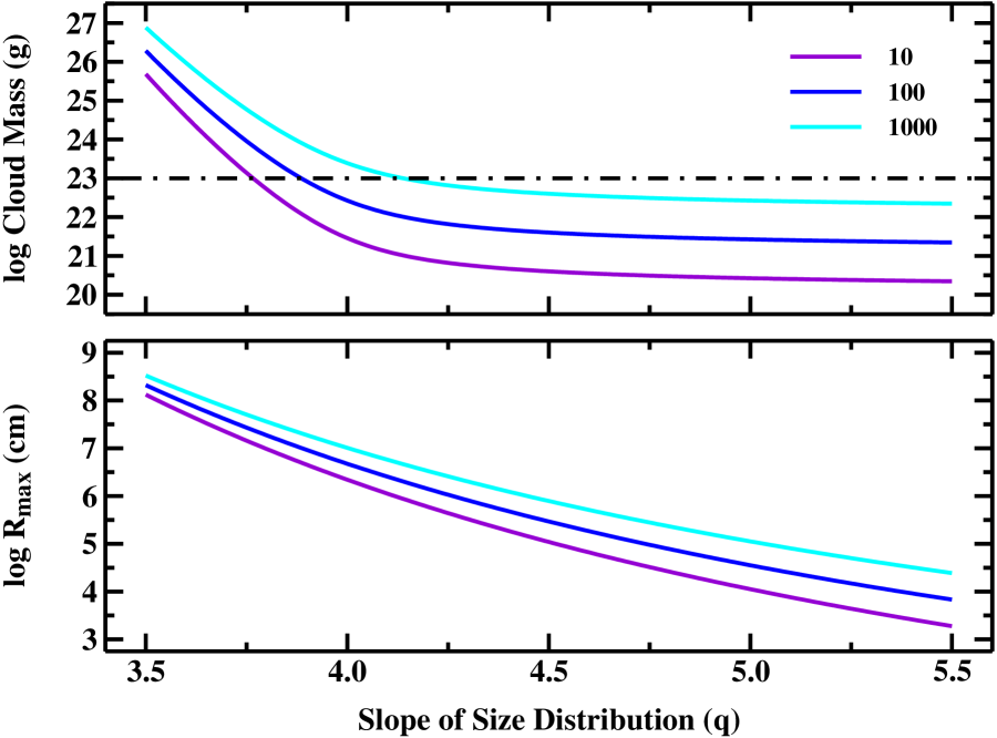
Figure 12: Size of the largest object $R_{max}$ (lower panel) and cloud mass $M_{d}$ (upper panel) as a function of the slope of the size distribution $q$ for $A_{d}$ = $10^{23}$ cm² and various $R_{min}$ (in $\rm\mu{\rm m}$) as indicated in the legend. The horizontal dot-dashed line in the upper panel shows the maximum possible cloud mass from the capture model (eq. [LABEL:eq:_mdot-cap]). Matching the observed $A_{b}$ with $M_{d}$ $\lesssim 10^{23}$ g requires $q\gtrsim$ 4 and $R_{max}$ $\lesssim$ 50–60 km.

To derive combinations of $R_{max}$ and $q$ where $A_{d}=A_{b}\approx$ $10^{23}$ cm² with $M_{d}\ \lesssim 10^{23}$ g, we set $R_{min}$ = 10–1000 $\rm\mu{\rm m}$ and calculate $R_{max}$ and $M_{d}$ as a function of $q$ (Fig. 12). For clouds with $q\lesssim$ 3.9, the mass required to match the observed $A_{b}$ exceeds the likely maximum amount of captured material, $\sim 10^{23}$ g. These models fail. When $q\approx$ 4, clouds with $R_{max}$ $\approx$ 30–50 km and $M_{d}\ \approx 10^{22}-10^{23}$ g yield the observed area. Clouds with $q\approx$ 4.5–5.5 have $R_{max}$ $\approx$ 0.1–1 km and total masses $M_{d}\ \approx 10^{21}$ g.

As the cross-sectional area of a cloud approaches $A_{d}\approx 10^{23}$ cm², the long-term evolution depends on collision outcomes, collision rates, and the total angular momentum. Captured fragments typically have semimajor axis $a_{f}\approx\gamma R_{H}$ and large eccentricity $e_{f}\gtrsim$ 0.3. If the distribution of inclination angles relative to the plane of the circumstellar disk is random, each fragment has a randomly oriented angular momentum vector with specific angular momentum $L_{f}\approx(Gma_{f}(1-e_{f}^{2}))^{1/2}$ (e.g., Dones & Tremaine, 1993). On average, the total angular momentum is zero with a standard deviation of roughly $\sqrt{N}L_{f}$. If the planet captures material with somewhat higher or lower specific angular momentum than the planet, captured material may have a significant total angular momentum (Dones & Tremaine, 1993).

For captured particles with a range of radii, collision outcomes are sensitive to particle size. Particles in a roughly spherical cloud have typical collision velocity $v\approx 1.3(GM_{p}/a_{f})^{1/2}$ (e.g., Kennedy & Wyatt, 2011, and references therein). Collisions with large kinetic energy relative to the binding energy produce debris; small collision energies allow mergers. For R $\gtrsim$ 0.01 km, the binding energy grows rapidly with radius. Thus, collisions add mass to large particles and remove mass from small particles. To identify the boundary between these regimes for collisions between unequal mass particles, we set $M_{esc}/M_{2}\gtrsim 1$ in eq. (10):

$$R_{d,u}\lesssim 7\left({M_{p}\over 1~{}M_{\oplus}\ }\right)^{1/3}~{}.$$ (16)

For collisions among equal mass particles, setting $M_{esc}/M_{tot}\lesssim$ 0.1 in eq. (14) yields a similar relation:

$$R_{d,e}\lesssim 5\left({M_{p}\over 1~{}M_{\oplus}\ }\right)^{1/2}~{}.$$ (17)

For planets with $M_{p}\approx$ 0.1–10 $M_{\oplus}$, objects with $R\gtrsim$ 5–10 km grow slowly with time. Collisions destroy all smaller particles.

Particle sizes also set the collision rates. The typical lifetime of a 100 $\rm\mu{\rm m}$ particle is short

$$t_{s}\approx 5\times 10^{3}\left({10^{23}~{}{\rm cm^{2}}\over A_{d}}\right)~{}{\rm yr}~{}.$$ (18)

On this time scale, collisions convert 100 $\rm\mu{\rm m}$ particles into much smaller particles which are unstable to radiation pressure. These collisions reduce the mass and cross-sectional area of the cloud.

For 10 km objects, the typical lifetime is much longer,

$$t_{l}\approx 5\times 10^{6}\left({10^{23}~{}{\rm cm^{2}}\over A_{d}}\right)~{}{\rm yr}~{}.$$ (19)

Throughout their lifetimes, these large objects continually replenish the supply of much smaller objects. Although the cloud mass remains roughly constant, collisions among large objects increase the cross-sectional area of the cloud.

For the nominal capture rate in eq. (LABEL:eq:_mdot-cap), the typical lifetime of 10 km objects implies a low mass cloud with a steep size distribution. If captures replenish the cloud on a $5\times 10^{6}$ yr time scale, the cloud has a typical mass $M_{d}\approx 5\times 10^{21}$ g. Larger (smaller) capture rates allow a larger (smaller) cloud mass. To match the nominal $M_{d}$ and $A_{d}$ for $R_{min}$ = 100 $\rm\mu{\rm m}$, the size distribution has $R_{max}$ $\lesssim$ 100 km and $q\gtrsim$ 4.

Although factor of ten changes to $R_{min}$ have little impact on our conclusions (Fig. 12), changing the capture rate allows a broader range of possible matches to observations. Larger (smaller) capture rates imply shallower (steeper) size distributions with larger (smaller) $R_{max}$. Thus, matching the observed $A_{b}$ with factor of 10–1000 increases in the capture rate is possible with $q=$ 3.9–3.5. However, reducing the capture rate by a factor of 10 or more eliminates all power-law size distributions with $R_{min}\gtrsim$ 30 $\rm\mu{\rm m}$. In these situations, the cloud mass is too small to match the observed $A_{b}$.

3.3.3 Summary

This discussion establishes an evolutionary sequence for a capture model in Fomalhaut b. We envision a long series of protoplanet collisions within the Hill sphere of a much larger planet. These collisions gradually produce a cloud of satellites orbiting the planet, with sizes ranging from $R_{min}$ $\sim$ 100 $\rm\mu{\rm m}$ up to $R_{max}$ $\approx$ 10–20 km. As the mass of the cloud grows, collisions among captured objects eventually produce a collisional cascade where objects with $R\lesssim$ 5 km are slowly ground into smaller and smaller objects. Continuous captures from the circumstellar disk maintain the population of 1–5 km objects.

Although larger objects grow throughout this evolution, they accrete a modest fraction of the cloud mass. For $q\approx$ 4.0–4.5, the typical 10–20 km object doubles its mass every 50–200 Myr. Over the lifetime of Fomalhaut, continuous capture of material allows the satellites to reach maximum sizes of roughly 100 km, comparable to the sizes of the irregular satellites of the giant planets in the solar system (e.g., Bottke et al., 2010; Kennedy & Wyatt, 2011).

Within this picture, there are several necessary components for a successful capture model with $A_{d}=A_{b}\approx 10^{23}$ cm².

• Fomalhaut b must pass through regions of the disk with $d\approx$ 0.3–1.0. Otherwise, an Earth-mass planet cannot capture enough material for the nominal $f_{cap}\approx 2\times 10^{-3}$. At Fomalhaut b’s current position inside the orbit of the bright dust belt, the average surface density of the circumstellar disk is probably a factor of 3–5 lower than the bright belt (Acke et al., 2012). Thus, $d\lesssim$ 0.1–0.2. In this environment, Earth-mass planets may not accumulate enough material to produce an observable cross-sectional area of small particles. If Fomalhaut b passes through the dust belt, it encounters regions with $d\approx$ 0.5–1.0 and can capture a significant amount of material. Thus, the capture model is more viable if Fomalhaut b passes through the dust belt.

• Captures and collisional evolution within the cloud must maintain a size distribution with $q\gtrsim$ 4.0–4.5. Otherwise, planets cannot capture enough mass to achieve the observed cross-sectional area. Within a standard collisional cascade, $q\lesssim$ 3.8–3.9 (O’Brien & Greenberg, 2003; Kobayashi & Tanaka, 2010). However, impacts of 10–100 km objects often produce debris with $q\approx$ 4–6 (e.g., Durda et al., 2004; Leinhardt & Stewart, 2012). It seems plausible that a size distribution produced from both processes will have an intermediate $q\approx$ 4.0–4.5.

Given existing data for Fomalhaut and Fomalhaut b, these conditions are achievable. The most likely orbit for Fomalhaut b has $e\gtrsim$ 0.5 and may pass through the bright belt of debris (Kalas et al., 2013; Beust et al., 2014). This orbit enables an Earth-mass planet to capture material into a large cloud orbiting the planet. A rough balance between captures and collisional grinding then yields a cross-sectional area $A_{d}=A_{b}\approx 10^{23}$ cm². Thus, capture is a viable model for dust in Fomalhaut b.

Aside from the ability of an Earth-mass planet to capture sufficient material, the main uncertainty in this picture is whether captures and collisional grinding can produce a steep size distribution with $q\approx$ 4.0–4.5. If these processes produce a shallower size distribution with $q\lesssim$ 4.0, clouds of captured particles will have a much smaller surface area than observed in Fomalhaut b. We return to these issues in §4.

3.4 Collisional Cascade within a Circumplanetary Cloud or Disk

A collisional cascade is a reliable way to produce a long-lived cloud of dust around a planet (see, for example, Kennedy & Wyatt, 2011; Wyatt, 2008, and references therein). In this picture, a disk or a roughly spherical cloud of solids orbits the planet. Destructive collisions among small satellites lead to a cascade of collisions which eventually grinds small particles into dust. The largest satellites are often immune to destruction. These satellites may slowly remove material from the cloud until collisions and radiation pressure remove all of the smaller objects.

To explain dust emission in Fomalhaut b, we consider two variants of the collisional cascade picture. We assume a cloud or disk of material with initial mass $M_{d}$, particle sizes ranging from $R_{min}$ to $R_{max}$, and a power-law size distribution with slope $q$. Following (Kennedy & Wyatt, 2011), collisions drive the evolution. Captures from the circumstellar disk are neglected (for an illustration of evolution with an initially massive disk and captures, see Bottke et al., 2010). For either model, a massive swarm of particles ensures a large cross-sectional area for small dust grains and a long lifetime for the collisional cascade. Within a circumplanetary disk, a large satellite with $R\gtrsim$ 500 km stirs the smaller satellites and maintains high collision velocities. Without this satellite, collisional damping among the smaller satellites reduces collision velocities and halts the cascade (e.g., Kenyon & Bromley, 2002). Although large satellites are plausible constituents of a roughly spherical cloud (e.g., Bottke et al., 2010; Kennedy & Wyatt, 2011), they are not vital for maintaining the cascade.

The properties of a circumplanetary cloud or disk depend on the collision model. The main parameters in this model are $q$, $R_{max}$, $R_{min}$, the mass $M_{p}$ of the planet, the orbital semimajor axis $a$ and the eccentricity $e$ of the planet, and the mass $M_{\star}$ and luminosity $L_{\star}$ of the central star (e.g., Kennedy & Wyatt, 2011, and references therein). To explore a large portion of the available parameter space with minimal constraints, we consider a simple picture where destructive collisions of objects with radii $R$ drive the collisional cascade. We assume all collisions produce an array of fragments. In this model, the lifetime of the largest particle is then the collision time, $t_{coll}\approx\rho RPV/M_{d}$, where $V$ is the volume of the cloud or disk and $P$ is the orbital period. Although this approach is much simpler than the collision model in Kennedy & Wyatt (2011), it follows the spirit of more detailed discussions and yields similar results for cloud and disk geometries.

To evaluate this expression, we assign $r$ = 120 AU and $M_{\star}$ = 2 $M_{\odot}$. We assume the swarm extends to a distance $a_{max}\approx\gamma R_{H}$ from the planet, where $\gamma\approx$ 0.3 (e.g., Hamilton & Burns, 1992; Toth, 1999; Shen & Tremaine, 2008; Martin & Lubow, 2011). Adopting the appropriate volume for a cloud or disk, we express the collision time in terms of the dust mass:

$$t_{coll}\approx 9\left({R\over{\rm 1~{}km}}\right)\left({{0.01~{}M_{\oplus}}\over M_{d}}\right)\left({\gamma\over 0.3}\right)^{7/2}\left({r\over{\rm 120~{}AU}}\right)^{7/2}\left({M_{p}\over{10~{}M_{\oplus}}}\right)^{2/3}\left({{2~{}M_{\odot}}\over M_{\star}}\right)^{7/6}~{}{\rm Myr}.$$ (20)

For swarms containing 1% of an Earth mass orbiting a 10 $M_{\oplus}$ planet, destructive collisions among objects with $R\approx$ 50–100 km yield lifetimes of 400–800 Myr. Thus, the cascade can survive for the $\sim$ 400 Myr age of Fomalhaut (Mamajek, 2012; Mamajek et al., 2013).

Estimating the dust mass in eq. (20) requires $q$ and $R_{min}$. Here, we expand on Kennedy & Wyatt (2011) and examine several plausible values. In an equilibrium cascade, the predicted slope of the size distribution is $q\approx 3.5-3.7$ (e.g., O’Brien & Greenberg, 2003; Kobayashi & Tanaka, 2010). To allow some flexibility, we set $q\approx$ 3.5–3.9. For this range in $q$, most of the mass is in the largest objects; most of the cross-sectional area is in the smallest objects. As noted in §3.3, the minimum stable radius for a single particle orbiting a 1–10 $M_{\oplus}$ planet is roughly 100–300 $\rm\mu{\rm m}$ (Kennedy & Wyatt, 2011). To examine the impact of $R_{min}$, we set $R_{min}$ $\approx$ 30–300 $\rm\mu{\rm m}$.

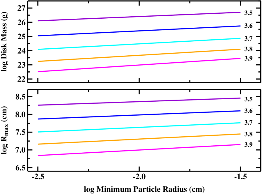
Figure 13: Circumplanetary disk mass and maximum satellite radius as a function of $R_{min}$ and $q$ for a collisional cascade surrounding a massive planet. Ensembles of particles with $q\lesssim$ 3.7 and cross-sectional area $A_{d}\ =10^{23}$ cm² have the large maximum radius, $R_{max}$ $\gtrsim$ 300 km, necessary to maintain a collisional cascade.

To derive $M_{d}$, we set $A_{d}=A_{b}\approx 10^{23}$ cm² and calculate $R_{max}$ as a function of $q$ and $R_{min}$ (eqs. [8–9]). Fig. 13 shows the result. For the nominal parameters, $q\approx$ 3.5 and $R_{min}$ = 300 $\rm\mu{\rm m}$, the mass of the swarm is $M_{d}\approx$ 0.01 $M_{\oplus}$. The expected collision time is then several times the age of Fomalhaut. At fixed $q$, the mass is relatively insensitive to $R_{min}$, falling to $M_{d}\approx$ 0.003 $M_{\oplus}$ when $R_{min}\ \approx$ 30 $\rm\mu{\rm m}$. At fixed $R_{min}$, however, the dust mass is very sensitive to $q$. For reasonable $q\approx$ 3.6 (3.7), the mass falls to $M_{d}\approx$ 0.001 $M_{\oplus}$ ($M_{d}\approx 10^{-4}$ $M_{\oplus}$). Collision times for swarms orbiting 10 $M_{\oplus}$ planets are then very long. Because collision times for small particles are very short, maintaining the cascade is then difficult. However, increasing the mass of the central planet shortens the collision time and enables a robust collisional cascade throughout the main sequence lifetime of Fomalhaut.

Placing better constraints on the cascade requires a numerical simulation of collisional evolution in a circumplanetary cloud or disk (e.g., Bottke et al., 2010; Kenyon & Bromley, 2014). Although evolutionary calculations are cpu intensive, they provide a more robust measure of the size distribution, including sizes where $q$ can change dramatically (e.g., Kenyon & Bromley, 2004). Direct orbit calculations also yield better limits on $R_{min}$ and the area (e.g., Poppe & Horányi, 2011).

Here, we take advantage of the scalability of published calculations to make an independent estimate for the collisional lifetime of a circumplanetary disk around Fomalhaut b. As in eq. (20), the lifetime scales with the ratio of the orbital period to the surface density in the outer disk. Scaling results for circumstellar disks around solar-type stars (e.g., Kenyon & Bromley, 2008, 2010) and for circumplanetary disks around Pluto-Charon (Kenyon & Bromley, 2014) yields – remarkably – nearly identical time scales (to within a factor of two):

$$t_{coll-scale}\approx 100\left({{0.01~{}M_{\oplus}}\over M_{d}}\right)\left({m\over{10~{}M_{\oplus}}}\right)^{2/3}~{}{\rm Myr}~{}.$$ (21)

The calculations explicitly derive the growth of large objects; thus, the expression is independent of $R$. This collision time agrees well with our simple estimate in eq. (20). Thus, the conclusions derived for the properties of the debris are robust.

3.4.1 Summary

Our simple estimates for the collision time suggest a collisional cascade is a promising model for dust emission in Fomalhaut b (e.g., Kennedy & Wyatt, 2011; Galicher et al., 2013). Scaling results for the collision time from detailed evolutionary calculations of collisional cascades confirms this conclusion. Although continuously replenished during the cascade, the small dust particles in a massive circumplanetary debris disk have a large cross-sectional area for long time scales.

Our results for $R_{max}$ and $q$ illustrate the likely range in the mass of a cloud or a disk which can produce the measured cross-sectional area in Fomalhaut b. For $R_{min}$ $\approx$ 100 $\rm\mu{\rm m}$, the maximum radius of the size distribution changes from $R_{max}$ $\sim$ 1000 km for $q$ = 3.5 to $R_{max}$ $\approx$ 30 km for $q$ = 3.9. The plausible range in the dust mass is equally large: $\sim$ 0.01 $M_{\oplus}$ ($q$ = 3.5) to $\sim 10^{-5}$ $M_{\oplus}$ ($q$ = 3.9).

These constraints set strong limits on the masses of the central planet (e.g., Kennedy & Wyatt, 2011; Galicher et al., 2013). For $q$ = 3.5, swarms with 0.01 $M_{\oplus}$ of solid material orbiting a 10 $M_{\oplus}$ planet produce the observed area in Fomalhaut b for the likely main sequence lifetime of Fomalhaut. Although increasing the slope of the size distribution to $q=$ 3.7 (3.9) enables smaller masses, long collision lifetimes require a more massive planet, $m\approx 100~{}M_{\oplus}$ ($m\approx 1000~{}M_{\oplus}$). Current near-IR observations allow sub-Jupiter mass planets, but not super-Jupiter mass planets (Janson et al., 2012; Currie et al., 2012, 2013). Thus, current data preclude systems with $q\gtrsim 3.9$.

4 DISCUSSION

In §3, we considered three generic models – impacts, captures, and collisional cascades – for the origin of a cloud of dust in Fomalhaut b. In the simplest model, a single giant impact within the circumstellar disk produces an expanding cloud of dust orbiting the central star. As another simple alternative, dynamical processes during the earliest stages of planet formation leave a massive cloud or disk of solid particles surrounding a planet. Collisions among the largest satellites maintain a swarm of dust particles around the planet. The capture model is an interesting combination of these ideas, where a planet continuously captures the debris from giant impacts within its Hill sphere. If the cloud of debris becomes massive enough, a balance between material gained through capture and lost by a collisional cascade sets the properties of the circumplanetary dust cloud. Each of these models makes predictions for the mass and cross-sectional area of the dust cloud. Our analysis in §3 establishes these predictions.

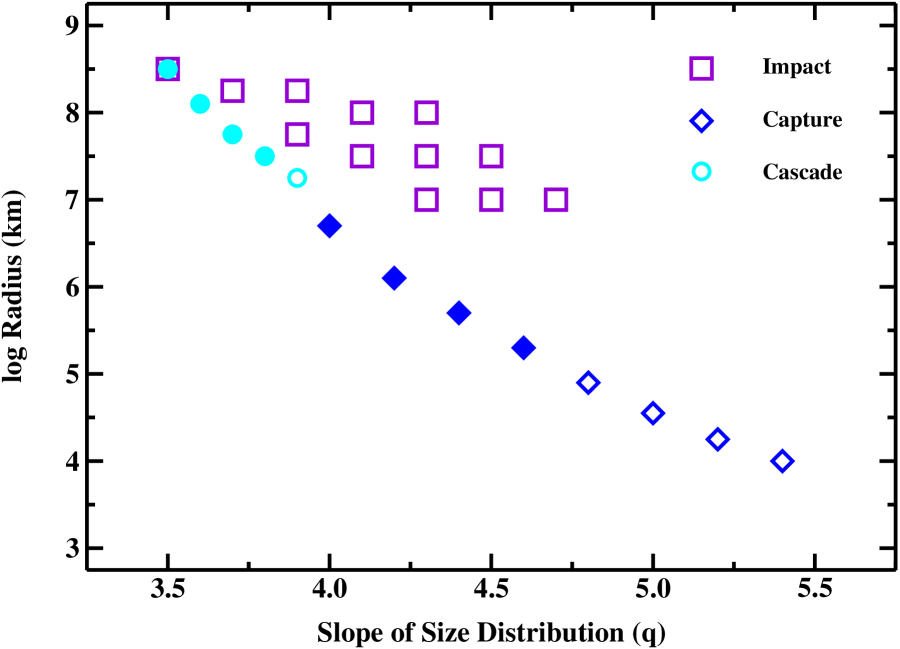
Figure 14: Combinations of $q$ and radius ($R_{max}$ for captures and cascades; $R_{1}$ for impacts) which can produce the observed cross-sectional area $A_{b}\approx 10^{23}$ cm² for models of giant impacts (violet points), captures (blue points), and collisional cascades (cyan points). Open symbols show combinations of $q$ and $R_{max},R_{1}$ which match the observed area. Filled circles indicate physically plausible combinations. Among allowed impact models, collisions are either too rare (large $R_{1}$) or require unlikely $q$ (small $R_{1}$). For captures and cascades, estimates for the cloud lifetime favor small $q$ and large $R_{max}$.

To summarize the constraints on each model, we collect the derived parameters for the slope of the dust size distribution ($q$) and the maximum radius of the size distribution ($R_{max}$, for captures and cascades) or the radii of two impactors ($R_{1}$). For simplicity, we consider steps of 0.2 in $q$ and 0.25 in log radius. The open symbols in Fig. 14 show combinations of $q$ and $R_{max},R_{1}$ which match the observed $A_{b}\approx 10^{23}$ cm².

Although the allowed parameter space is broad, simple physical arguments limit the parameter space considerably. For giant impact models (§3.2), collisions among pairs of objects with $R\gtrsim$ 100 km happen too rarely. Collisions among smaller objects occur more often, but standard collision outcomes produce debris with too little cross-sectional area to match observations. Non-standard outcomes with little debris in large particles can match the observed area with large $q$. Current numerical experiments of collisions suggest this option is improbable (e.g., Durda et al., 2004; Leinhardt & Stewart, 2012). Thus, giant impacts seem an implausible way to produce a dust cloud in Fomalhaut b.

Capture models appear somewhat more viable (§3.3). Earth-mass planets orbiting Fomalhaut at 120 AU can attract up to $10^{23}$ g of solids in 100 Myr. If this material maintains a steep size distribution, then the cross-sectional area of the cloud matches observations of Fomalhaut b. Although many combinations of $q$ and $R_{max}$ yield a model $A_{d}$ which can match the observed $A_{b}$ for $M_{d}$ $\approx 10^{21}-10^{23}$ g, the collision time precludes models with $q\gtrsim$ 4.6. When $q$ is too large, the largest particles have short collision times. Short collision times limit the mass of the cloud to $M_{d}\lesssim 10^{21}$ g, which is insufficient to produce the observed $A_{b}$ with $R_{min}$ $\approx$ 10–1000 $\rm\mu{\rm m}$. With this constraint, we limit the allowed parameter space to the four filled diamonds in Fig. 14.

Collisional cascade models are also reasonable (§3.4, see Kennedy & Wyatt, 2011). Within the allowed parameter space, size distributions with $R_{max}$ $\gtrsim$ 500 km can maintain the cascade for the age of Fomalhaut. In systems with smaller $R_{max}$ and larger $q$, there is too little material in the most massive objects. Thus, the cascade cannot survive for the 200–400 Myr age of Fomalhaut. Discounting these options limits the allowed parameter space to the three filled circles in Fig. 14.

Within $(q,R_{max})$ space, there are two main regions. Collisional cascade models permit $q\approx$ 3.5–3.7 and $R_{max}\approx$ 500–3000 km. Systems with smaller $q$ require larger $R_{max}$. Capture models allow $q\approx$ 4.0–4.6 and $R_{max}\approx$ 2–50 km. Systems with smaller $q$ require larger total mass. Both of these pictures require 1–10 Earth-mass planets. Our analysis strongly favors these options over a giant impact. Plausible giant impacts occur too rarely, require unlikely collision outcomes, or both.

These conclusions generally agree with previously published results. For giant impacts, Kalas et al. (2005) and Tamayo (2013) derive similarly low probabilities for collisions among 100–1000 km objects. Although Galicher et al. (2013) revise the collision probability upward, their estimate is based on the surface density of material within the belt. Given the newly measured trajectory of Fomalhaut b (Kalas et al., 2013; Beust et al., 2014) and the short lifetime of the debris cloud, any giant impact capable of producing Fomalhaut b must occur at distances $r\lesssim$ 120 AU where the surface density is at least a factor of six smaller than in the belt (§2.1). Thus, the Galicher et al. (2013) estimate of the collision frequency is overly optimistic.

Compared to Galicher et al. (2013), our approach to the outcomes of high velocity collisions between two protoplanets yields more ejected mass but less surface area. By using approximations appropriate for cratering collisions between a small object and a much larger one, Galicher et al. (2013) underestimate dust production from collisions between objects with roughly equal masses (§3.2). With the ejected mass known, Galicher et al. (2013) set $R_{min}$, $R_{max}$, and $q=3.5$ to yield the observed area. Our estimates for $A_{d}$ hinge on numerical experiments which derive the size of the largest fragment as a function of the ejected mass. After associating the size of the largest fragment with $R_{max}$, we derive $A_{d}$ as a function of $q$. Despite the larger ejected mass, this approach yields much larger $R_{max}$ and much smaller $A_{d}$. Given current collision theory (e.g., Leinhardt & Stewart, 2012, and references therein), our results seem more realistic. Discriminating between the two methods requires new numerical experiments of high velocity collisions.

Coupled with recent dynamical results, our collision analysis in §3.2 enables stronger limits on the impact hypothesis. Tamayo (2013) infers that collisions between two large objects are unlikely to lead to the large $e$ orbit in Fomalhaut b. He favors a collision between a small planetesimal and a much larger protoplanet already on a large $e$ orbit. However, collisions between one small and one large object produce enough dust only when the large object has $R\gtrsim$ 1000 km (§3.2). These collisions are very unlikely. Along with the need to produce the apparent apsidal alignment of Fomalhaut b and the main belt, these constraints challenge our ability to develop a viable impact model (e.g., Tamayo, 2013; Beust et al., 2014).

Capture models applied to Fomalhaut b have a limited history. Kennedy & Wyatt (2011) consider capture of material which strikes the central planet and ejects dust from the planet’s surface. Based on our analysis, we agree with their conclusion that the cross-section of a 1–10 $M_{\oplus}$ planet is too small to accrete enough mass for the Fomalhaut b dust cloud. Our results in §3.3 generally confirm their estimates for the amount of mass ejected in the collision. In our picture, the larger cross-section of the Hill sphere enables a larger capture rate. Both approaches ignore likely captures from circumstellar material striking orbiting satellites (Durda & Stern, 2000; Stern, 2009; Poppe & Horányi, 2011); this process likely adds captured material to the circumplanetary environment. Addressing the viability of this model in more detail requires numerical simulations.

Finally, we agree with previous studies supporting the collisional cascade model (Kennedy & Wyatt, 2011; Galicher et al., 2013; Kalas et al., 2013; Tamayo, 2013). Most studies derive similar properties for the central planet, 1–100 $M_{\oplus}$, and the surrounding circumplanetary cloud, $\sim$ 0.01 $M_{\oplus}$. The stability, surface area, and lifetime of the cloud set the lower mass limit on the planet (Kennedy & Wyatt, 2011; Galicher et al., 2013); minimizing disruption of the main dust belt sets the upper mass limit (Chiang et al., 2009; Kennedy & Wyatt, 2011; Tamayo, 2013; Beust et al., 2014). Our approach expands the allowed range of slopes for the size distribution of particles in a circumplanetary cloud or disk. Because the slope correlates with the dust mass, future dynamical studies can provide additional constraints on these parameters.

To explore the available parameter space for these models in more detail, we now examine plausible uncertainties (§4.2), tests (§4.3), and improvements (§4.4) of our approach.

4.1 Uncertainties

4.1.1 Observations

To examine how uncertainties impact our results, we begin with the derivation of the cross-sectional area from the observations. As outlined in §2, we assume that all radiation from Fomalhaut b is scattered light from Fomalhaut. The minimum cross-sectional area is then derived from the ratio of the scattered flux to the flux from Fomalhaut. The uncertainty is these quantities is small, $\sim$ 10%. Thus, the uncertainty in the minimum cross-sectional area is small.

Establishing an upper limit on the cross-sectional area requires an accurate estimate for the optical depth. Our analysis in §2.5 safely precludes $\tau\gtrsim$ 1 for giant impact models. Optically thick clouds orbiting a massive planet have collision times roughly $10^{10}$ times shorter than the age of Fomalhaut, robustly eliminating this possibility. With $\tau\lesssim$ 1, the observed $A_{b}$ yields an accurate estimate of the true $A_{b}$.

Deriving the true cross-sectional area of the dust requires an estimate of the albedo $Q$. Among Kuiper belt objects in the solar system, the albedo is typically $Q\approx$ 0.04–0.20 (Marcialis et al., 1992; Roush et al., 1996; Stansberry et al., 2008; Brucker et al., 2009). Choosing $Q\approx$ 0.1 thus yields a reasonable estimate for the actual cross-sectional area, $A_{b}\approx 1.25\times 10^{23}$ cm², with a factor of two uncertainty.

This uncertainty has little impact on our results (e.g., Fig. 6). For configurations with large $R_{max}$/$R_{min}$, changing $A_{b}$ by a factor of 2 modifies $M_{d}$ by a factor of $2^{2/3}$ = 1.6. For giant impacts with fixed $q$, this uncertainty implies a 20% variation in the derived target radius, a factor of two difference in the collision rate, and minimal revision to our conclusions. If the target radius is held fixed, a factor of two uncertainty in $A_{b}$ implies a 0.1–0.2 change in $q$. We infer similar adjustments to $q$ and $R_{max}$ for captures or collisional cascades. Thus, allowing for observational error in the cross-sectional area leads to minimal changes in the allowed parameter space of Fig. 14.

4.1.2 Size Distribution

On the theoretical side, we assume that the size distribution is a power law with a slope $q$ and a clear minimum size $R_{min}$ and maximum size $R_{max}$. Adopting a single largest remnant in a giant impact is reasonable. In a collisional cascade, the largest objects resist erosion by accreting smaller objects (e.g., Kenyon & Bromley, 2008, 2010, 2012). For the slopes inferred from our analysis, the next two largest objects have radii $R\approx$ 0.75–0.85 $R_{max}$ and $R\approx$ 0.65–0.75 $R_{max}$. Thus, a single largest object is appropriate for impact, capture, and cascade models.

Establishing the proper $R_{min}$ is somewhat more involved. When giant impacts yield small dust grains orbiting Fomalhaut at $r\approx$ 100 AU, setting the minimum radius equal to or larger than the blowout radius – $R_{min}$ $\gtrsim$ 5 $\rm\mu{\rm m}$ – is sensible. If small ($R\lesssim R_{min}$), icy grains at 120 AU have impurities of carbon or silicates, radiation pressure probably ejects them on the orbital or a smaller time scale (Artymowicz, 1988; Gustafson, 1994).

Independent of their total mass, grains with $R\lesssim R_{min}$ probably contain a large fraction of the cross-sectional area of the ejecta. With velocities much larger than the escape velocity of the impactors, they produce a rapidly expanding halo around the main ejecta. While visible for several years, very small grains become invisible on time scales much longer than a decade (e.g., Galicher et al., 2013; Kalas et al., 2013).

For capture and cascade models, isolated small particles are ejected when radiation pressure overcomes the gravity of the planet. For $M_{p}\approx$ 1–10 $M_{\oplus}$, $R_{min}$ $\approx$ 300 $\rm\mu{\rm m}$ (Burns et al., 1979; Kennedy & Wyatt, 2011). Although smaller particles might participate in the collisional processing of either mechanism, typical collision times are much longer than the planet’s orbital period. Thus, particles with $R\lesssim R_{min}$ leave after several orbits of the planet around Fomalhaut (Poppe & Horányi, 2011).

For impact models, adding more complexity to the size distribution is not warranted. As long as there is a broad range of sizes between $R_{min}$ and $R_{max}$, a single power-law provides a reasonably good way to relate the cross-sectional area, the mass, and the parameters – $q$, $R_{min}$, and $R_{max}$ – of the size distribution. Thus, this uncertainty seems minimal.

For viable capture models, a single power-law may not completely characterize the size distribution from 100 $\rm\mu{\rm m}$ to 50–100 km. In our picture, capturing the fragments of giant impacts yields a steep size distribution with $q\gtrsim 4$ (e.g., Durda et al., 2004; Leinhardt & Stewart, 2012). Collisional evolution among fragments tends to produce shallower size distributions with $q\approx$ 3.5–3.7 (O’Brien & Greenberg, 2003; Kobayashi & Tanaka, 2010). While a single power-law may not capture all details of capture and collisional evolution, it is probably sufficient to establish allowed values for $q$ and $R_{max}$.

In collisional cascades, the proper equilibrium size distribution is uncertain (e.g., Belyaev & Rafikov, 2011, and references therein). However, it is somewhat inaccurate to adopt a single power-law to describe the numbers of objects from a few microns to a few thousand kilometers. In long-term numerical simulations of cascades, the size distribution is better represented by separate power-laws at small ($R\lesssim$ 0.1–1  km), intermediate ($R\approx$ 1–100 km), and large sizes ($R\gtrsim$ 10–100 km; e.g., Kenyon & Bromley, 2004; Kenyon et al., 2008; Bottke et al., 2010; Kenyon & Bromley, 2012). Analytic studies support this conclusion (Pan & Sari, 2005; Schlichting et al., 2013). Wavy patterns are often superimposed on these power-laws (e.g., Campo Bagatin et al., 1994; O’Brien & Greenberg, 2003; Belyaev & Rafikov, 2011). The slopes of the power laws for the small and large objects are similar, with $q_{S}\approx 3.5-4.0$ and $q_{L}\approx$ 2.5–4.5; the slope of the intermediate power law is small, with $q_{I}\approx$ -1 to 1. Observations of Kuiper belt objects in the solar system reveal fairly strong evidence for a break in the size distribution at $\sim$ 20–100 km (e.g., Fuentes & Holman, 2008; Fraser et al., 2010) and some evidence for another break at small radii (e.g., Schlichting et al., 2012). Observed slopes are generally consistent with theoretical predictions (Bottke et al., 2010; Kennedy et al., 2011; Schlichting et al., 2012).

Quantifying how a somewhat wavy, multi-component power law approximation to the size distribution impacts our conclusions requires exploring a vast parameter space. To place an initial limit, we examine a few general cases for a typical outcome, $q_{S}\approx$ 3.5–4.0 and $q_{I}\approx$ 1. Compared to models of a single size distribution with $q\approx$ 3.5–3.7 and $R_{max}$ $\approx$ 500–3000 km, multiple power laws with $q_{L}>q_{S}$ match the observed $A_{b}$ with an $R_{max}$ which is larger by a factor of 1.5–2. When $q_{L}<q_{S}$, matching $A_{b}$ requires a steeper slope, with $q_{S}\approx q+\delta q$ and $\delta q\approx$ 0.4–0.5. Because the intermediate part of the size distribution contains little area or mass, multiple power law models require a factor of 2–4 more mass to achieve the same surface area.

Although a factor of 2–4 uncertainty in the mass certainly impacts the size distribution and the lifetime of a collision cascade (e.g., Wyatt, 2008; Kenyon & Bromley, 2008; Krivov et al., 2008; Kennedy & Wyatt, 2010; Kenyon & Bromley, 2010), it has little impact on the general viability of collisional cascade models. From eq. (20), the collision time scales inversely with the mass and linearly with $M_{p}^{2/3}$. For a fixed cascade lifetime, changing the mass involved in the cascade requires a corresponding adjustment to $M_{p}$. With current observations requiring $M_{p}\lesssim 0.5M_{J}$, it is fairly straightforward to adjust the mass required for the collisional cascade and meet the broad range of allowed planet masses.

4.1.3 Collision Physics

Aside from the physical parameters of the size distribution, the physics of collisions and collision outcomes plays a major role in our analysis. Our results for impacts hinge on understanding debris production during collisions between large objects. Analyses of captures and cascades also rely on swarms of solid particles finding stable equilibrium size distributions over long periods of time.

Although each mechanism depends on an accurate parameterization of the binding energy of icy objects, the uncertainties in $Q_{D}^{\star}$ probably have little impact on our results. In a collisional cascade, satellites lose mass when the collision energy exceeds $Q_{D}^{\star}$ (e.g., Dohnanyi, 1969; O’Brien & Greenberg, 2003; Kenyon & Bromley, 2008; Kobayashi & Tanaka, 2010). Because $Q_{c}$ varies with the orbital velocity, it is possible to compensate for changes in $Q_{D}^{\star}$ simply by changing the mass of the planet. For a reasonably large range in planet masses, the subsequent evolution of the cascade is largely unchanged.

The binding energy has little impact on capture models. In our picture, $Q_{D}^{\star}$ helps to set the collision time for the largest objects (eqs. [16–19]). Although factor of two uncertainties in $Q_{D}^{\star}$ can lead to similar uncertainties in the rate particles lose mass, the collision time for the largest objects depends mainly on the cross-sectional area. Thus, our assumptions for $Q_{D}^{\star}$ have a relatively small, $\sim$ 10% to 20%, impact on the collision time and the total mass of the cloud.

Viable impact models are more sensitive to $Q_{D}^{\star}$. Changing $Q_{D}^{\star}$ by a factor of two changes debris production by a similar factor. Less debris (larger $Q_{D}^{\star}$) makes giant impacts less viable. Although more debris adds to the viability of giant impacts, these models still require steep size distributions with little mass in the largest remnant. These outcomes are still unlikely.

Our assumption of a head-on giant impact has little impact on our conclusions. When impacts are off-center, the center-of-mass impact energy is smaller by a factor $b$, the impact parameter (e.g., Asphaug et al., 2006; Leinhardt & Stewart, 2012; Stewart & Leinhardt, 2012). With less energy available in a collision and the same energy required to unbind half the colliding protoplanets, off-center collisions lose less mass than head-on collisions. Thus, allowing for off-center collisions reduces the likelihood that a giant impact is responsible for the dust in Fomalhaut b.

For captures and cascades, the outcomes of collisions have little impact on the results. For sizes where collisions produce destruction or growth, the rate particles diminish or grow depends on the collision rate much more than collision outcomes (Kobayashi & Tanaka, 2010; Kobayashi et al., 2010, 2011). Simple physics constrains the collision rates.

Our conclusions for giant impacts rely heavily on the published outcomes of numerical experiments of high energy collisions (e.g., Benz & Asphaug, 1999; Durda et al., 2004; Leinhardt & Stewart, 2012). So far, different approaches yield similar results: high velocity collisions between objects with substantial self-gravity always leave behind large remnants with a significant fraction of the debris. Because the dust cloud in Fomalhaut b appears to require debris with little mass in the largest remnants, a large impact seems an unlikely way to produce the dust cloud. If numerical simulations identify collision parameters capable of producing the debris required in Fomalhaut b, an impact becomes much more plausible.

4.1.4 Orbital Dynamics

Finally, several aspects of orbital dynamics might modify our conclusions. In a planet with a highly elliptical orbit, for example, the size of the Hill sphere is smaller at periastron than at apoastron. Satellites with circumplanetary orbits at semimajor axes of 0.3–0.4 $R_{H}$ might be stable at apoastron but unstable at periastron. Because these satellites have orbital periods comparable to the orbital period of Fomalhaut b around Fomalhaut, it should take many Fomalhaut b orbits to develop unstable satellite orbits (e.g., Shen & Tremaine, 2008). Indeed, Kalas et al. (2013) showed that planets with $M_{p}\gtrsim 5\times 10^{24}$ g on Fomalhaut b-like orbits can retain satellites with semimajor axes of 0.3–0.4 $R_{H}$. Thus, the elliptical orbit has little impact on the stability of captured satellites or satellites involved in a collisional cascade.

Dynamical interactions among satellites also play a role in the viability of capture and collisional cascade models. In an ensemble of satellites, gravitational interactions produce random velocities comparable to the escape velocity of the largest satellite (e.g., Goldreich et al., 2004). When these random velocities exceed the orbital velocity, satellites are ejected. In the transneptunian region of the solar system, these interactions produce the scattered disk – an ensemble of 10–500 km icy objects with perihelia near the orbit of Neptune and large orbital eccentricity (e.g., Gladman et al., 2008).

Managing the cascade around 1–10 $M_{\oplus}$ planets with much larger satellites is challenging. Massive satellites with $R\approx$ 500–1500 ${\rm km~{}s^{-1}}$ have escape velocities, $v_{esc}\approx$ 0.5–1.5 ${\rm km~{}s^{-1}}$, much larger than the local orbital velocity. On a few dynamical time scales, these objects eject smaller satellites orbiting within 2–3 Hill radii (e.g., Gladman, 1993; Goldreich et al., 2004), which is roughly 0.05–0.06 AU. For a satellite system with an outer radius of 0.25–0.5 AU, 5–10 massive satellites can eject all small objects on very short time scales.

Maintaining a roughly spherical cloud of dust in a capture or cascade model is also challenging. For any initial geometry, energy loss and angular momentum transport from inelastic collisions eventually produce a prograde disk with angular momentum similar to the initial angular momentum of the cloud (Brahic, 1976). If the initial orbits within the cloud are roughly balanced between prograde and retrograde, material gradually falls onto the planet instead of landing in a large disk. This evolution probably enhances the mass loss rate from a roughly spherical collisional cascade, shortening the lifetime.

4.2 Tests

The simplest ways to deduce the source of the optical emission in Fomalhaut b involve polarimetry or spectroscopy. Imaging polarimetry excels at probing the underlying geometry of dusty clouds or disks (e.g., Whitney & Hartmann, 1993; Whitney et al., 1997; Olofsson et al., 2012). Optical or IR spectroscopy might reveal absorption features from the central A-type star (Lagrange et al., 1995; Hempel & Schmitt, 2003) or silicate features from dust (Telesco & Knacke, 1991; Weinberger et al., 2003). Measuring the velocity of cloud material with high resolution spectroscopy (e.g., Olofsson et al., 2001; Brandeker et al., 2004) would discriminate between expanding and orbiting geometries. Unfortunately, these observations are far in the future. The HST and the James Webb Space Telescope (JWST) have no polarimetric capabilities. Although the source is too faint for HST spectroscopy, the prototype exposure time calculator for NIRSPEC on JWST yields an 8$\sigma$ detection for an A-type continuum with an exposure time of 3600 sec. Although JWST is scheduled for launch no sooner than 2018, low resolution NIRSPEC spectra may enable accurate tests of dust models for Fomalhaut b.

Extending photometry to longer wavelengths also tests these models (e.g., Currie et al., 2012, 2013). JWST NIRCAM observations will enable better than 10$\sigma$ detections at 1–3 $\rm\mu{\rm m}$ (e.g., Tamayo, 2013). On a somewhat longer time scale, ground-based imaging with 20-m to 40-m class telescopes might provide independent measures of the spectral energy distribution at 1–5 $\rm\mu{\rm m}$.

Until JWST launches, other approaches are possible. To develop tests for giant impact models, we assume an unbound cloud of dust particles with an expansion velocity exceeding the escape velocity of a pair of impactors with $R\approx$ 50 km, $v_{esc}\approx 5-6\times 10^{3}~{}{\rm cm~{}s^{-1}}$.

• Expansion of the cloud is detectable on short time scales. If all of the material expands at $v_{esc}$, the expansion rate is roughly 0.01 AU yr^-1 (e.g., Galicher et al., 2013; Kalas et al., 2013). However, the ejecta probably have a range of velocities with $f(>v)\propto(v/v_{esc})^{-\alpha}$ (Gault et al., 1963; Stoeffler et al., 1975; Housen & Holsapple, 2003, 2011). Adopting $\alpha$ = 1.5, roughly 20% (50%) of the material has $v\gtrsim 3~{}v_{esc}$ ($1.6~{}v_{esc}$). If 35% of the dust expands at twice $v_{esc}$, the diameter grows roughly 0.4 AU (1–2 pixels on HST images) in 10 yr. Although current efforts to resolve the source are inconclusive (e.g., §2; Galicher et al., 2013; Kalas et al., 2013), improving the resolution and placing robust limits on the expansion rate should be possible in the next decade (e.g., Tamayo, 2013).

• Shearing of the cloud is also detectable. For particles expanding at median velocity $v$ from a guiding center with orbital velocity $v_{K}$, the velocity dispersion is roughly $\delta v\approx v$ (e.g., Gault et al., 1963; Housen & Holsapple, 2003). Among particles expanding tangentially to the orbital motion, some lag the orbit; others move ahead of the orbit. Thus, the sphere shears into a ring (e.g., Kenyon & Bromley, 2005). When $\delta v/v_{K}\approx v/v_{K}\approx 0.01-0.02$, the differential motion is $\delta r/r\approx 0.01-0.02$. Over 10 yr, the guiding center moves roughly 8 AU (Kalas et al., 2013), resulting in a predicted shear of 0.15–0.3 AU. In the next decade, HST and JWST data can test this prediction.

  Our large estimate for the shearing rate – a few decades instead of 100–1000 yr (Currie et al., 2012; Galicher et al., 2013; Kalas et al., 2013; Tamayo, 2013) – is based on the larger internal velocity dispersion of debris clouds suggested by laboratory and numerical experiments. Performing SPH simulations of collisions between pairs of 50–200 km objects (e.g., Leinhardt & Stewart, 2012) in a Keplerian reference frame would test these ideas.

• Collisions with other circumstellar disk particles enhance these rates. For a typical relative velocity of 0.4 ${\rm km~{}s^{-1}}$, it takes roughly 10 yr for a disk particle to cross the cloud. During this period, one in $10^{3}$ disk particles collides with a cloud particle. If the surface density of the disk at $r\approx$ 120 AU is 1% to 10% ($d=0.01-0.10$) of the initial surface density, roughly $10^{21}$ g to $10^{22}$ g of disk material mixes with particles in the expanding cloud every decade. Because orbits in the disk differ from orbits of the cloud, these collisions enhance the rate of expansion and orbital shear by factors of three or more.

  Even very modest amounts of mixing – $\sim 10^{18}$ g, corresponding to a disk with $d\approx 10^{-5}$ – can easily increase the expansion and shear by roughly 50%. Any mixing thus increases the chances of detecting expansion or shearing very soon. If Fomalhaut b enters the dust belt (Galicher et al., 2013; Kalas et al., 2013), the enhanced collision rate should produce an obvious shear on very short time scales.

Without high quality polarimetry or spectroscopy, robust tests of the capture or cascade pictures are more challenging. Still, several tests allow promising tests of either scenario.

• Although significant expansion or contraction of captured or cascading material is unlikely, measurements of Fomalhaut b’s size place important constraints on the models. As noted in §2, unambiguous resolution of the disk of Fomalhaut b places a robust lower limit on the mass of a central planet.

• Placing better limits on the azimuthal structure of material at 20–130 AU also constrains models for Fomalhaut b. If dust in the inner disk is smoothly distributed (as in the model of Acke et al., 2012), capture models are more viable. Detecting patchy dust increases the likelihood of massive planets in the inner disk and decreases the likelihood of significant capture of small solids by planets in the inner disk.

• Collisional cascades should leave behind a trail of small particles (e.g., Kalas et al., 2013). Because particles with $R\approx$ 5–300 $\rm\mu{\rm m}$ are blown out of circumplanetary – but not circumstellar – orbits, these particles should take up orbits along the path of Fomalhaut b. Assuming 10$\sigma$ detections from existing observations of Fomalhaut b, the brightest detectable cloud of small dust particles is a factor of 5–10 fainter than Fomalhaut b. With roughly 1000 resolution elements along the elliptical orbit, it is possible to discriminate a trail from the background if an ensemble of small dust particles has a total cross-sectional area $A_{d,s}\approx 1000/5-10\approx$ 100–200 times the cross-sectional area of the dust observed in Fomalhaut b. If it is possible to coadd data convincingly in an annulus along the orbit, a robust algorithm could detect fainter trails.

  Although there are many uncertainties, this level of emission from 5–300 $\rm\mu{\rm m}$ particles is plausible. For size distributions with $q\approx$ 3.5–4.0, the cross-sectional area of the small particles is 7–20 times larger than the area of the circumplanetary debris disk. If the particles do not drift too far away from the orbit and if collisions do not destroy small particles ejected well before the current epoch, it is possible to enhance this surface area by factors of 3–10 (see, for example Wyatt, 2008; Kenyon & Bromley, 2008, 2010; Kennedy & Wyatt, 2010, 2011, and references therein). Unambiguous limits on this trail would enable stern tests of capture and cascade models.

• Fomalhaut b’s possible entry into Fomalhaut’s dust belt provides another opportunity to test cascade (e.g., Kalas et al., 2013) and capture models. By analogy with Saturn’s rings (e.g., Durisen et al., 1989) and Kuiper belt objects (e.g., Stern, 2009), we expect several classes of behavior when particles from the dust belt interact with circumplanetary dust: (i) large objects from the belt will carry away small circumplanetary particles and (ii) collisions between small belt objects and large circumplanetary objects will produce debris. For small objects in a captured cloud or disk, entry into the dust ring will be dramatic: we expect an initial loss of captured material on 10 yr time scales, followed by a slow increase as the rare collisions of larger objects produce debris which repopulates the smaller sizes. Because collisional cascades have a shallower dust distribution, we expect much less dramatic changes: as large objects remove small particles from the cloud or the disk, collisions between larger objects rapidly restore lost material. The time scale for any variations, however, should be similar, $\sim$ 10–100 yr.

4.3 Improvements

As observations continue to probe the nature of Fomalhaut b, new approaches can hone theoretical predictions. Although clear improvements in analytic approaches are possible, here we outline several numerical calculations to clarify expectations.

For all dust models, it is crucial to add to our understanding of interactions between the dust cloud and ambient material in the disk. If the surface density of the disk at 30–100 AU is roughly 1% to 10% of the initial surface density, then disk material inevitably interacts with the cloud. From our earlier estimates, disk material with a total mass comparable to the mass of the cloud interacts with cloud material every 10–100 yr (for impact and capture models) to every $10^{4}-10^{5}$ yr (for cascade models). If these interactions add material to the cloud, they make (i) capture and cascade models more viable and (ii) impact models less viable. Interactions which remove material from the cloud tend to decrease the viability of all models.

Despite the wealth of analytic and numerical work (e.g., Dones & Tremaine, 1993; Kortenkamp, 2005; Jewitt & Haghighipour, 2007; Nesvorný et al., 2007; Pires dos Santos et al., 2012), estimating the amount of material a planet can capture throughout the history of a planetary system remains uncertain. For Fomalhaut b, its elliptical orbit through the inner disk and main belt of dust might lead to substantial differences in the capture rate. Numerical simulations can place stronger constraints on our simple estimates.

Numerical experiments could clarify the long-term collisional evolution of circumplanetary debris. Our estimates for the viability of the capture hypothesis rest on the development of an equilibrium between the rate captures add mass to the cloud and the rate collisions remove mass from the cloud. More sophisticated calculations can address this issue.

Finally, numerical calculations can illuminate the relative importance of cloud and disk geometries for collisional cascades around massive planets. During the early evolution of the solar system, dynamical interactions between the gas giants strongly favor cloud geometries for swarms of captured particles (e.g., Nesvorný et al., 2007). In a dynamically quiet environment, however, growing planets might easily capture large disks of particles. Unless these disks are disrupted by the gravity of another massive planet, massive satellite formation and the onset of a collisional cascade is inevitable. Understanding common features and differences of circumplanetary cascades in clouds and disks might enable new tests of the cascade model.

5 SUMMARY

We explore the ability of three generic models – giant impacts, captures, and collisional cascades – to account for a large dust cloud in Fomalhaut b. After deriving the basic observational constrains (§2), we develop a novel approach to the power-law size distribution of solid particles (§3.1) and apply this technique to giant impacts (§3.2), captures (§3.3), and collisional cascades (§3.4). Despite the uncertainties in our approach (§4.1), we derive several clear constraints.

1. Giant impacts seem the least plausible model (for another approach for rejecting this picture, see Tamayo, 2013). Although it is possible to produce enough debris in a collision between two 100 km objects, the outcome required to match the observations is unlikely. However, this model is the easiest to test: simple theory expects detectable expansion and shearing of the belt in the next decade (e.g., Galicher et al., 2013; Kalas et al., 2013).

2. Although capture models are viable, it is challenging to produce a stable cloud or disk of captured particles which lasts for the main sequence lifetime of Fomalhaut. If small particles contain most of the mass, planets can capture enough material from the inner disk and main belt of Fomalhaut to produce the observed cross-sectional area. We speculate that these systems can find an equilibrium size distribution from captures and collisional evolution. More detailed calculations can test this idea.

3. A collisional cascade is the least problematic model. In principle, Earth-mass or larger planets with reasonable circumplanetary reservoirs of solid material can maintain a cascade for the main sequence lifetime of Fomalhaut. However, it is unclear whether the system can reach the required equilibrium between damping and stirring (e.g., Kennedy & Wyatt, 2011).

4. Although testing the capture and cascade models, both should leave detectable trails of small particles along their orbits. Current data – or images acquired with JWST – might reveal these trails.

Within the next decade, observations with HST or JWST can test these models. Detecting image expansion/shear or a trail of small particles along Fomalhaut b’s orbit is possible with either facility. IR spectroscopy with JWST would provide a direct measure of the amount of scattered light from a dust cloud. If Fomalhaut b passes through the main belt, comparing time variations in brightness with the predictions of more detailed theoretical calculations should also constrain the models.

Whatever the nature of Fomalhaut b, it gives us new insights into collisional evolution and planet formation theory. As the observational constraints grow, we are likely to learn more about the outcomes of individual collisions and the evolution of swarms of solid particles.

Comments from M. Geller and a thoughtful referee improved our presentation. Portions of this project were supported by the NASA Astrophysics Theory and Origins of Solar Systems programs through grant NNX10AF35G and the NASA Outer Planets Program through grant NNX11AM37G.

Table 1: Fomalhaut b Data

Telescope/Instrument	Filter	$\lambda$ ($\mu m$)	Apparent Magnitude	Flux Density ($\mu$Jy)	Reference
HST/ACS	F435W	0.435	25.22 $\pm$ 0.18	0.32 $\pm$ 0.06	1
”	F606W	0.606	24.95 $\pm$ 0.13	0.36 $\pm$ 0.04	1
”	F814W	0.814	24.91 $\pm$ 0.20	0.27 $\pm$ 0.05	1
HST/STIS	50CORO	0.574	24.96 $\pm$ 0.20	0.38 $\pm$ 0.08	2
HST/WFC3	F110W	1.15	–	$<$ 1.60	3
Subaru/IRCS	J	1.25	$>$ 22.22	$<$ 3.36	1
Keck/NIRC2	H	1.65	$>$ 22.60	$<$ 0.94	4
Spitzer/IRAC	$[3.6]$	3.6	$>$ 13.82	$<$ 833	5
Spitzer/IRAC	$[4.5]$	4.5	$>$ 16.66	$<$ 38.80	6
Spitzer/IRAC	$[5.8]$	5.8	$>$ 11.32	$<$ 3416	5
Spitzer/IRAC	$[8.0]$	8	$>$ 11.12	$<$ 2317	5

Note. — References: 1) Currie et al. (2012), 2) This work, 3) Galicher et al. (2013), 4) Currie et al. (2013), 5) Marengo et al. (2009), 6) Janson et al. (2012). Upper limits for non-detections are quoted as 5-$\sigma$ upper limits. For the F606W photometery, we use the average of the 2004 and 2006 measurements: 24.92 $\pm$ 0.10 and 24.97 $\pm$ 0.09. The HST/STIS filter central wavelength refers to the pivot wavelength listed in the fits header.

Table 2: Fomalhaut b Spatial Extent Estimates in ACS Data

Data Set	FWHM (pt. source)	FWHM (linear fit) [x,y]	FWHM (gaussian fit) [x,y]
	milliarcsec	milliarcsec	milliarcsec
F435W	50	[56 $\pm$ 15, 69 $\pm$ 14]	[59 $\pm$ 13, 71 $\pm$ 18]
F606W (2004)	69	[75 $\pm$ 13, 80 $\pm$ 17]	[68 $\pm$ 13, 75 $\pm$ 13]
F606W (2006)	69	[69 $\pm$ 14, 57 $\pm$ 15]	[69 $\pm$ 14, 56 $\pm$ 15]
F814W	94	[120 $\pm$ 60, 65 $\pm$ 25]	[108 $\pm$ 25, 60 $\pm$ 30]

References

- Acke et al. (2012) Acke, B., et al. 2012, A&A, 540, A125
- Agnor & Hamilton (2006) Agnor, C. B., & Hamilton, D. P. 2006, Nature, 441, 192
- Andrews et al. (2013) Andrews, S. M., Rosenfeld, K. A., Kraus, A. L., & Wilner, D. J. 2013, ApJ, 771, 129
- Artymowicz (1988) Artymowicz, P. 1988, ApJ, 335, L79
- Asphaug et al. (2006) Asphaug, E., Agnor, C. B., & Williams, Q. 2006, Nature, 439, 155
- Barrado y Navascues (1998) Barrado y Navascues, D. 1998, A&A, 339, 831
- Belyaev & Rafikov (2011) Belyaev, M. A., & Rafikov, R. R. 2011, Icarus, 214, 179
- Benz & Asphaug (1999) Benz, W., & Asphaug, E. 1999, Icarus, 142, 5
- Beust et al. (2014) Beust, H., et al. 2014, A&A, 561, A43
- Boley et al. (2012) Boley, A. C., Payne, M. J., Corder, S., Dent, W. R. F., Ford, E. B., & Shabram, M. 2012, ApJ, 750, L21
- Bottke et al. (2010) Bottke, W. F., Nesvorný, D., Vokrouhlický, D., & Morbidelli, A. 2010, AJ, 139, 994
- Brahic (1976) Brahic, A. 1976, Journal of Computational Physics, 22, 171
- Brandeker et al. (2004) Brandeker, A., Liseau, R., Olofsson, G., & Fridlund, M. 2004, A&A, 413, 681
- Brucker et al. (2009) Brucker, M. J., Grundy, W. M., Stansberry, J. A., Spencer, J. R., Sheppard, S. S., Chiang, E. I., & Buie, M. W. 2009, Icarus, 201, 284
- Burns et al. (1979) Burns, J. A., Lamy, P. L., & Soter, S. 1979, Icarus, 40, 1
- Campo Bagatin et al. (1994) Campo Bagatin, A., Cellino, A., Davis, D. R., Farinella, P., & Paolicchi, P. 1994, Planet. Space Sci., 42, 1079
- Canup (2004) Canup, R. M. 2004, Icarus, 168, 433
- Canup (2005) —. 2005, Science, 307, 546
- Canup (2011) —. 2011, AJ, 141, 35
- Canup & Asphaug (2001) Canup, R. M., & Asphaug, E. 2001, Nature, 412, 708
- Chiang et al. (2009) Chiang, E., Kite, E., Kalas, P., Graham, J. R., & Clampin, M. 2009, ApJ, 693, 734
- Currie et al. (2013) Currie, T., Cloutier, R., Debes, J. H., Kenyon, S. J., & Kaisler, D. 2013, ApJ, 777, L6
- Currie et al. (2012) Currie, T., et al. 2012, ApJ, 760, L32
- Davis et al. (1985) Davis, D. R., Chapman, C. R., Weidenschilling, S. J., & Greenberg, R. 1985, Icarus, 63, 30
- Dohnanyi (1969) Dohnanyi, J. S. 1969, J. Geophys. Res., 74, 2531
- Dones & Tremaine (1993) Dones, L., & Tremaine, S. 1993, Icarus, 103, 67
- Durda et al. (2004) Durda, D. D., Bottke, W. F., Enke, B. L., Merline, W. J., Asphaug, E., Richardson, D. C., & Leinhardt, Z. M. 2004, Icarus, 170, 243
- Durda & Stern (2000) Durda, D. D., & Stern, S. A. 2000, Icarus, 145, 220
- Durisen et al. (1989) Durisen, R. H., Cramer, N. L., Murphy, B. W., Cuzzi, J. N., Mullikin, T. L., & Cederbloom, S. E. 1989, Icarus, 80, 136
- Estrada & Mosqueira (2006) Estrada, P. R., & Mosqueira, I. 2006, Icarus, 181, 486
- Fraser et al. (2010) Fraser, W. C., Brown, M. E., & Schwamb, M. E. 2010, Icarus, 210, 944
- Fuentes & Holman (2008) Fuentes, C. I., & Holman, M. J. 2008, AJ, 136, 83
- Galicher et al. (2013) Galicher, R., Marois, C., Zuckerman, B., & Macintosh, B. 2013, ApJ, 769, 42
- Gault et al. (1963) Gault, D. E., Shoemaker, E. M., & Moore, H. J. 1963, NASA Tech. Note, D-1767
- Giacomuzzo et al. (2007) Giacomuzzo, C., Ferri, F., Bettella, A., Pavarin, D., Francesconi, A., Flamini, E., & Angrilli, F. 2007, Advances in Space Research, 40, 244
- Gillett (1986) Gillett, F. C. 1986, in Astrophysics and Space Science Library, Vol. 124, Light on Dark Matter, ed. F. P. Israel, 61–69
- Gladman (1993) Gladman, B. 1993, Icarus, 106, 247
- Gladman et al. (2008) Gladman, B., Marsden, B. G., & Vanlaerhoven, C. 2008, in The Solar System Beyond Neptune, ed. Barucci, M. A., Boehnhardt, H., Cruikshank, D. P., & Morbidelli, A. (University of Arizona Press, Tucson, AZ), 43–57
- Goldreich et al. (2002) Goldreich, P., Lithwick, Y., & Sari, R. 2002, Nature, 420, 643
- Goldreich et al. (2004) —. 2004, ARA&A, 42, 549
- Greenberg et al. (1978) Greenberg, R., Hartmann, W. K., Chapman, C. R., & Wacker, J. F. 1978, Icarus, 35, 1
- Gustafson (1994) Gustafson, B. A. S. 1994, Annual Review of Earth and Planetary Sciences, 22, 553
- Hamilton & Burns (1992) Hamilton, D. P., & Burns, J. A. 1992, Icarus, 96, 43
- Hamilton & Krivov (1997) Hamilton, D. P., & Krivov, A. V. 1997, Icarus, 128, 241
- Hempel & Schmitt (2003) Hempel, M., & Schmitt, J. H. M. M. 2003, A&A, 408, 971
- Heng & Tremaine (2010) Heng, K., & Tremaine, S. 2010, MNRAS, 401, 867
- Holland et al. (2003) Holland, W. S., et al. 2003, ApJ, 582, 1141
- Housen & Holsapple (2003) Housen, K. R., & Holsapple, K. A. 2003, Icarus, 163, 102
- Housen & Holsapple (2011) —. 2011, Icarus, 211, 856
- Janson et al. (2012) Janson, M., Carson, J. C., Lafrenière, D., Spiegel, D. S., Bent, J. R., & Wong, P. 2012, ApJ, 747, 116
- Jewitt (2012) Jewitt, D. 2012, AJ, 143, 66
- Jewitt & Haghighipour (2007) Jewitt, D., & Haghighipour, N. 2007, ARA&A, 45, 261
- Kalas et al. (2005) Kalas, P., Graham, J. R., & Clampin, M. 2005, Nature, 435, 1067
- Kalas et al. (2013) Kalas, P., Graham, J. R., Fitzgerald, M. P., & Clampin, M. 2013, ArXiv e-prints
- Kalas et al. (2008) Kalas, P., et al. 2008, Science, 322, 1345
- Kennedy & Wyatt (2010) Kennedy, G. M., & Wyatt, M. C. 2010, MNRAS, 405, 1253
- Kennedy & Wyatt (2011) —. 2011, MNRAS, 412, 2137
- Kennedy et al. (2013) Kennedy, G. M., Wyatt, M. C., Kalas, P., Duchêne, G., Sibthorpe, B., Lestrade, J.-F., Matthews, B. C., & Greaves, J. 2013, MNRAS
- Kennedy et al. (2011) Kennedy, G. M., Wyatt, M. C., Su, K. Y. L., & Stansberry, J. A. 2011, MNRAS, 417, 2281
- Kenyon & Bromley (2002) Kenyon, S. J., & Bromley, B. C. 2002, AJ, 123, 1757
- Kenyon & Bromley (2004) —. 2004, AJ, 128, 1916
- Kenyon & Bromley (2005) —. 2005, AJ, 130, 269
- Kenyon & Bromley (2008) —. 2008, ApJS, 179, 451
- Kenyon & Bromley (2010) —. 2010, ApJS, 188, 242
- Kenyon & Bromley (2012) —. 2012, AJ, 143, 63
- Kenyon & Bromley (2014) —. 2014, AJ, 147, 8
- Kenyon et al. (2008) Kenyon, S. J., Bromley, B. C., O’Brien, D. P., & Davis, D. R. 2008, in The Solar System Beyond Neptune, ed. Barucci, M. A., Boehnhardt, H., Cruikshank, D. P., & Morbidelli, A. (University of Arizona Press, Tucson, AZ), 293–313
- Kobayashi & Tanaka (2010) Kobayashi, H., & Tanaka, H. 2010, Icarus, 206, 735
- Kobayashi et al. (2011) Kobayashi, H., Tanaka, H., & Krivov, A. V. 2011, ApJ, 738, 35
- Kobayashi et al. (2010) Kobayashi, H., Tanaka, H., Krivov, A. V., & Inaba, S. 2010, Icarus, 209, 836
- Koch & Hansen (2011) Koch, F. E., & Hansen, B. M. S. 2011, MNRAS, 416, 1274
- Kortenkamp (2005) Kortenkamp, S. J. 2005, Icarus, 175, 409
- Krivov et al. (2008) Krivov, A. V., Müller, S., Löhne, T., & Mutschke, H. 2008, ApJ, 687, 608
- Lagrange et al. (1995) Lagrange, A. M., Vidal-Madjar, A., Deleuil, M., Emerich, C., Beust, H., & Ferlet, R. 1995, A&A, 296, 499
- Leinhardt & Stewart (2009) Leinhardt, Z. M., & Stewart, S. T. 2009, Icarus, 199, 542
- Leinhardt & Stewart (2012) —. 2012, ApJ, 745, 79
- Leinhardt et al. (2008) Leinhardt, Z. M., Stewart, S. T., & Schultz, P. H. 2008, in The Solar System Beyond Neptune, ed. Barucci, M. A., Boehnhardt, H., Cruikshank, D. P., & Morbidelli, A. (University of Arizona Press, Tucson, AZ), 195–211
- Lissauer (1987) Lissauer, J. J. 1987, Icarus, 69, 249
- Mamajek (2012) Mamajek, E. E. 2012, ApJ, 754, L20
- Mamajek et al. (2013) Mamajek, E. E., et al. 2013, AJ, 146, 154
- Marcialis et al. (1992) Marcialis, R. L., Lebofsky, L. A., Disanti, M. A., Fink, U., Tedesco, E. F., & Africano, J. 1992, AJ, 103, 1389
- Marengo et al. (2009) Marengo, M., Stapelfeldt, K., Werner, M. W., Hora, J. L., Fazio, G. G., Schuster, M. T., Carson, J. C., & Megeath, S. T. 2009, ApJ, 700, 1647
- Marsh et al. (2005) Marsh, K. A., Velusamy, T., Dowell, C. D., Grogan, K., & Beichman, C. A. 2005, ApJ, 620, L47
- Martin & Lubow (2011) Martin, R. G., & Lubow, S. H. 2011, MNRAS, 413, 1447
- Nesvorný et al. (2007) Nesvorný, D., Vokrouhlický, D., & Morbidelli, A. 2007, AJ, 133, 1962
- O’Brien & Greenberg (2003) O’Brien, D. P., & Greenberg, R. 2003, Icarus, 164, 334
- O’Keefe & Ahrens (1985) O’Keefe, J. D., & Ahrens, T. J. 1985, Icarus, 62, 328
- Olofsson et al. (2001) Olofsson, G., Liseau, R., & Brandeker, A. 2001, ApJ, 563, L77
- Olofsson et al. (2012) Olofsson, G., Nilsson, R., Florén, H.-G., Djupvik, A., & Aberasturi, M. 2012, A&A, 544, A43
- Pan & Sari (2005) Pan, M., & Sari, R. 2005, Icarus, 173, 342
- Pires dos Santos et al. (2012) Pires dos Santos, P. M., Morbidelli, A., & Nesvorný, D. 2012, Celestial Mechanics and Dynamical Astronomy, 114, 341
- Poppe & Horányi (2011) Poppe, A., & Horányi, M. 2011, Planet. Space Sci., 59, 1647
- Ricci et al. (2012) Ricci, L., Testi, L., Maddison, S. T., & Wilner, D. J. 2012, A&A, 539, L6
- Roush et al. (1996) Roush, T. L., Cruikshank, D. P., Pollack, J. B., Young, E. F., & Bartholomew, M. J. 1996, Icarus, 119, 214
- Ruskol (1961) Ruskol, E. L. 1961, Soviet Ast., 4, 657
- Ruskol (1963) —. 1963, Soviet Ast., 7, 221
- Ruskol (1972) —. 1972, Soviet Ast., 15, 646
- Schlichting et al. (2013) Schlichting, H. E., Fuentes, C. I., & Trilling, D. E. 2013, AJ, 146, 36
- Schlichting et al. (2012) Schlichting, H. E., et al. 2012, ApJ, 761, 150
- Shen & Tremaine (2008) Shen, Y., & Tremaine, S. 2008, AJ, 136, 2453
- Spiegel & Burrows (2012) Spiegel, D. S., & Burrows, A. 2012, ApJ, 745, 174
- Stansberry et al. (2008) Stansberry, J., Grundy, W., Brown, M., Cruikshank, D., Spencer, J., Trilling, D., & Margot, J.-L. 2008, in The Solar System Beyond Neptune, ed. Barucci, M. A., Boehnhardt, H., Cruikshank, D. P., & Morbidelli, A. (University of Arizona Press, Tucson, AZ), 161–179
- Stapelfeldt et al. (2004) Stapelfeldt, K. R., et al. 2004, ApJS, 154, 458
- Stern (2009) Stern, S. A. 2009, Icarus, 199, 571
- Stewart & Leinhardt (2012) Stewart, S. T., & Leinhardt, Z. M. 2012, ApJ, 751, 32
- Stoeffler et al. (1975) Stoeffler, D., Gault, D. E., Wedekind, J., & Polkowski, G. 1975, J. Geophys. Res., 80, 4062
- Su et al. (2013) Su, K. Y. L., et al. 2013, ApJ, 763, 118
- Suetsugu & Ohtsuki (2013) Suetsugu, R., & Ohtsuki, K. 2013, MNRAS, 431, 1709
- Suetsugu et al. (2011) Suetsugu, R., Ohtsuki, K., & Tanigawa, T. 2011, AJ, 142, 200
- Svetsov (2011) Svetsov, V. 2011, Icarus, 214, 316
- Tamayo (2013) Tamayo, D. 2013, ArXiv e-prints
- Tanaka et al. (1996) Tanaka, H., Inaba, S., & Nakazawa, K. 1996, Icarus, 123, 450
- Telesco & Knacke (1991) Telesco, C. M., & Knacke, R. F. 1991, ApJ, 372, L29
- Toth (1999) Toth, I. 1999, Icarus, 141, 420
- Weidenschilling (2002) Weidenschilling, S. J. 2002, Icarus, 160, 212
- Weinberger et al. (2003) Weinberger, A. J., Becklin, E. E., & Zuckerman, B. 2003, ApJ, 584, L33
- Wetherill & Stewart (1989) Wetherill, G. W., & Stewart, G. R. 1989, Icarus, 77, 330
- Whitney & Hartmann (1993) Whitney, B. A., & Hartmann, L. 1993, ApJ, 402, 605
- Whitney et al. (1997) Whitney, B. A., Kenyon, S. J., & Gomez, M. 1997, ApJ, 485, 703
- Williams & Wetherill (1994) Williams, D. R., & Wetherill, G. W. 1994, Icarus, 107, 117
- Williams & Cieza (2011) Williams, J. P., & Cieza, L. A. 2011, ArXiv e-prints
- Wyatt (2008) Wyatt, M. C. 2008, ARA&A, 46, 339
- Wyatt & Dent (2002) Wyatt, M. C., & Dent, W. R. F. 2002, MNRAS, 334, 589
- Youdin & Kenyon (2013) Youdin, A. N., & Kenyon, S. J. 2013, From Disks to Planets, ed. T. D. Oswalt, L. M. French, & P. Kalas, 1