Wideband Mosaic Imaging with the VLA - quantifying faint source imaging accuracy

Abstract

A large number of deep and wide-field radio interferometric surveys are being designed to measure accurate statistics of faint source populations. Most require mosaic observations, and expect to benefit from the sensitivity provided by broad-band instruments. In this paper, we present preliminary results from a comparison of several wideband imaging methods in the context of how accurately they reconstruct the intensities and spectral indices of micro-Jy level sources.

1 Introduction

The recent upgrade of the Very Large Array (VLA) has resulted in a greatly increased imaging sensitivity due to the availability of large instantaneous bandwidths at the receivers and correlator. A considerable amount of telescope time has been allotted for large survey projects that need deep and sometimes high dynamic range imaging over fields of view that span one or more primary beams. In this imaging regime, traditional algorithms have limits in the achievable dynamic range and accuracy with which weak sources are reconstructed. Narrow-band approximations of the sky brightness and instrumental effects result in sub-optimal continuum sensitivity and angular resolution. Narrow-field approximations that ignore the time-, frequency-, and polarization dependence of antenna primary beams prevent accurate reconstructions over fields of view larger than the inner part of the primary beam. Mosaics constructed by stitching together images reconstructed separately from each pointing often have a lower imaging fidelity than a joint reconstruction. Despite these drawbacks, all these methods are easy to apply using readily available and stable software and are therefore used regularly.

More recently-developed algorithms that address the above shortcomings also exist. Wide-band imaging algorithms (Sault et al., 1994; Rau et al., 2011) make use of the combined multi-frequency spatial frequency coverage while reconstructing both the sky intensity and spectrum at the same time. Wide-field imaging algorithms (Cornwell et al., 2008; Bhatnagar et al., 2008) include corrections for instrumental effects such as the w-term and antenna aperture illumination functions. Wideband A-Projection (Bhatnagar et al., 2013), a combination of the two methods mentioned above separates the frequency dependence of the sky from that of the instrument during wideband imaging. Finally, an algorithm to perform a joint mosaic reconstruction (Cornwell, T.J., 1998) along with a wideband sky model and wideband primary beam correction has recently been demonstrated to work accurately and is currently being commissioned (Rau et al., 2014)(in prep). These methods provide superior numerical results compared to traditional methods but they require all the data to be treated together during the reconstruction and need specialized software implementations that are optimized for the large amount of data transport and memory usage involved in each imaging run.

With so many methods to choose from and various trade-offs between numerical accuracy, computational complexity and ease of use, it becomes important to identify the most appropriate approach for a given imaging goal and to quantify the errors that would occur if other methods are used. This paper describes some preliminary results based on a series of simulated tests of deep wide-band and wide-field mosaic observations with the VLA.

2 Data Simulation

A sky model was chosen to contain a set of 8000 point sources spanning one square degree in area. Intensities ranged between $1\mu Jy$ and $7mJy$ plus one bright $100mJy$ source, and followed a realistic source count distribution. Spectral indices ranged between 0.0 and -0.8 with a peak in the spectral index distribution at -0.7 plus a roughly Gaussian distribution around -0.3 with a width of 0.5. This source list is a subset of that available from the SKADS/SCubed simulated sky project (Wilman et al., 2008).

Observations were simulated for a VLA mosaic at D-config and C-band with 46 pointings (of primary beams 6 arcmin in HPBW at 6 GHz) spaced 5 arcmin apart. 16 channels (or spectral windows) were chosen to span the frequency range of 4-8 GHz, and the $uv$-coverage corresponds to one pointing snapshot every 6 minutes, tracing the entire mosaic twice within 8.8 hours.

Visibilities were simulated per pointing, using the WB-A-Projection de-gridder (Bhatnagar et al., 2013) which used complex antenna aperture illumination functions to model primary beams that rotate with time, scale with frequency, and have polarization squint. No noise was added.

3 Imaging Algorithms

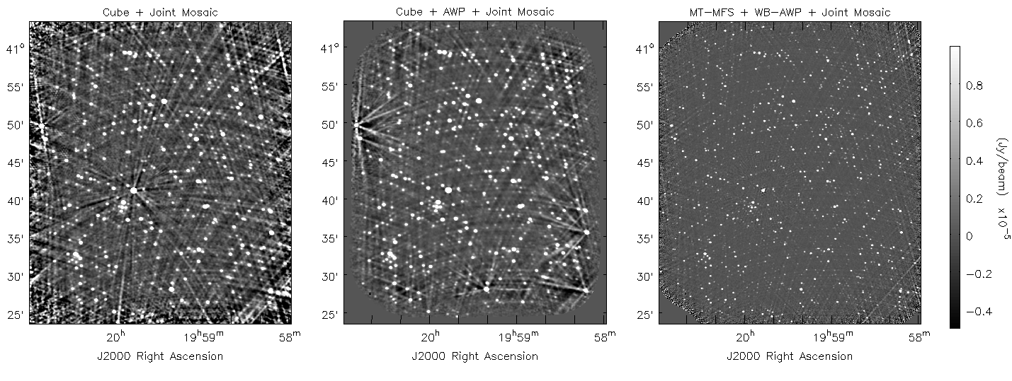
Figure 1: Restored continuum intensity images : (LEFT) Cube + Joint Mosaic, (MIDDLE) Cube + AWP + Joint Mosaic, (RIGHT) MT-MFS + WB-AWP + Joint Mosaic. Intensity range shown : $-5\mu Jy$ to $+10\mu Jy$.

The wideband mosaic dataset described above was imaged in a variety of ways. In all cases the data products were continuum intensity images and spectral index maps. Figure. 1 shows restored continuum mosaic images from the first, third and fifth algorithms described below.

1. Cube + Joint Mosaic : A joint mosaic reconstruction is performed separately per channel (spectral window). A mosaic primary beam correction is then done per channel, and all channels are smoothed to the angular resolution at the lowest frequency in the observation. Spectral models are then fit for each pixel/source and a weighted frequency average is done to form a continuum image.

2. Cube + AWP + Joint Mosaic : Same as above, but with narrow-band A-Projection per channel (spectral window) to account for beam rotation and squint.

3. MT-MFS + Stitched Mosaic : Each pointing is imaged separately using multi-term multi-frequency-synthesis followed by post-deconvolution wideband primary beam correction and adding all image patches together by weighting them by an average primary beam.

4. MT-MFS + WB-AWP + Stitched Mosaic: Each pointing is imaged separately using MT-MFS along with wideband A-Projection that eliminates the frequency dependence of the primary beam before the image modeling process. A post deconvolution correction of only the intensity image is required before a weighted average is done to combine images from all pointings.

5. MT-MFS + WB-AWP + Joint Mosaic : All data are imaged together, with a wideband sky model and antenna-, time-, frequency- and polarization-dependent primary beam correction during imaging with wideband A-Projection.

4 Tests and Results

The intensity and spectral index maps produced by the above algorithms were compared with the known simulated sky. For each output image, the simulated sky model image was first smoothed to match its angular resolution, and then pixel values were read off from both images at all the locations of the true source pixels. Histograms were plotted for $I/I_{true}$ where deviations from 1.0 indicate relative flux errors and for $\alpha-\alpha_{true}$ where deviations from 0.0 indicate relative errors in spectral index. All histograms were made with multiple intensity ranges and over different fields of view to look for trends in the errors. The mean and half-width of each of the resulting distributions (over different intensity ranges) for the first, third and fifth method described above are listed in Table 1. Spectral index reconstructions for the weakest sources $<5\mu Jy$ were not included as all the methods were inaccurate. These numbers show that cube methods have wider distributions for all intensity ranges. This is primarily because of weak sources that are not detected in single channel images but appear as confused undeconvolved sources in the continuum image. The achieved mean values in both intensity and spectral index show that accurate handling of the primary beam (via A-Projection) is required in order to recover the intensity and spectral index to within a few percent, particularly for weak sources. These results are part of a larger study (to be described in an upcoming publication) that includes single pointing tests to evaluate effects of sparse $uv$-coverage, the use of masks during deconvolution, the accuracy of beam polarization correction, a method to deal with undeconvolved sources in cube methods, sources not on pixel centers, baseline based averaging, visibility noise, and various choices and numerical approximations within the reconstruction algorithms.

Table 1: Intensity and Spectral Index reconstruction accuracy as a function of source intensity

Method	$I/I_{true}$	$I/I_{true}$	$I/I_{true}$	$\alpha-\alpha_{true}$	$\alpha-\alpha_{true}$
Intensity Range	$>20\mu Jy$	$5-20\mu Jy$	$<5\mu Jy$	$>50\mu Jy$	$10-50\mu Jy$
Cube	0.9 $\pm$ 0.1	0.9 $\pm$ 0.3	0.9 $\pm$ 0.5	-0.5 $\pm$ 0.2	-0.6 $\pm$ 0.5
Cube + AWP	1.0 $\pm$ 0.05	1.0 $\pm$ 0.2	1.0 $\pm$ 0.3	-0.15 $\pm$ 0.1	-0.1 $\pm$ 0.25
MTMFS + WB-AWP	1.0 $\pm$ 0.02	1.0 $\pm$ 0.04	1.0 $\pm$ 0.15	-0.05 $\pm$ 0.05	-0.1 $\pm$ 0.2

References

- Sault et al. (1994) Sault,R.J. & Wieringa,M., 1994, A&A Suppl.Ser, 108, 585
- Rau et al. (2011) Rau, U. & Cornwell, T. J., 2011, A&A, 532, A71
- Cornwell et al. (2008) Cornwell, T. J., Golap, K., Bhatnagar, S., 2008, IEEE Sel. Top. in Sig. Proc., vol2, 647-657
- Bhatnagar et al. (2008) Bhatnagar, S., Cornwell, T. J., Golap, K., Uson, J. M., 2008, A&A, vol 487, 419-429
- Bhatnagar et al. (2013) Bhatnagar, S., Rau, U, Golap, K., ApJ, 770, 91
- Cornwell, T.J. (1998) Cornwell, T. J., A&A, 202,316
- Rau et al. (2014) Rau, U., Bhatnagar, S., Golap, K., (in prep)
- Wilman et al. (2008) Wilman, R. J., Miller,L., Jarvis, M. J., Mauch, T., Levrier, F., Abdalla, F. B., Rawlings, S., Kl ckner, H. R., Obreschkow, D., Olteanu, D., Young, S, MNRAS, Vol 388, 1335-1348