Photon Regions and Shadows of Kerr–Newman–NUT Black Holes with a Cosmological Constant

Abstract

We consider the Plebański class of electrovacuum solutions to the Einstein equations with a cosmological constant. These space-times, which are also known as the Kerr–Newman–NUT–(anti-)de Sitter space-times, are characterized by a mass $m$, a spin $a$, a parameter $\beta$ that comprises electric and magnetic charge, a NUT parameter $\ell$ and a cosmological constant $\Lambda$. Based on a detailed discussion of the photon regions in these space-times (i.e., of the regions in which spherical lightlike geodesics exist), we derive an analytical formula for the shadow of a Kerr–Newman–NUT–(anti-)de Sitter black hole, for an observer at given Boyer–Lindquist coordinates $(r_{O},\vartheta_{O})$ in the domain of outer communication. We visualize the photon regions and the shadows for various values of the parameters.

I Introduction

Over the last twenty years observations have produced increasing evidence for the existence of a supermassive black hole at the center of our galaxy. This evidence comes from the observation of orbits of stars in the infrared EckartGenzel.1996 ; GillessenEisenhauerEtAl.2009 which allows to estimate the mass of the central object. In combination with estimates of the volume in which this mass must be concentrated the result strongly supports the hypothesis of a black hole. These observations are expected to become even more precise when the GRAVITY instrument EisenhauerEtAl.2009 goes into operation soon. In addition, it is planned to explore the inner region of the center of our galaxy, in the order of magnitude of the Schwarzschild radius of the central mass, with submillimeter radio telescopes. From this project, which is called the Event Horizon Telescope DoelemanWeintroub.2008 , we expect a radio image of the shadow of the central black hole in a few years’ time. Therefore, it is timely to advance the theoretical investigations of the shadows of black holes as far as possible, as a basis for evaluating the observational results that are to be expected soon.

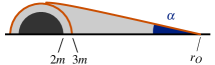
Figure 1: Angular radius $\alpha$ of the shadow of a Schwarzschild black hole, given by Synge’s formula, Eq. (1).

For an observer at radius coordinate $r_{O}$ in the Schwarzschild space-time, the shadow can be constructed in the following way. We assume that there are light sources distributed on the sphere $r=r_{L}$ for some chosen $r_{L}>r_{O}$. We consider all light rays issuing from the observer’s position into the past. Some of them will reach a light source at $r_{L}$, after being deflected by the black hole; to the initial directions of this first class of light rays we associate brightness on the observer’s sky. Some of them will go to the horizon and never reach a light source at $r_{L}$; to the initial directions of this second class of light rays we associate darkness on the observer’s sky. The second class fills the shaded region in Fig. 1. The borderline between the two classes are light rays that asymptotically spiral towards the photon sphere at $r=3m$ (with $G=1$, $c=1$). Therefore, in this case the shadow is circular and its angular radius is determined by light rays that approach the photon sphere, see again Fig. 1. For simplicity, we have constructed the shadow with light sources on a sphere $r=r_{L}$. From the geometry it is clear that we could have light sources anywhere else as long as they are outside of the shaded region in Fig. 1.

Synge Synge.1966 was the first to calculate what we nowadays call the shadow of a Schwarzschild black hole. (Synge did not use the word “shadow” but he investigated the condition under which photons could escape to infinity.) He found that the angular radius $\alpha$ of the shadow is given by the simple formula

$$\sin^{2}\alpha=\frac{27}{4}\;\frac{(\rho_{O}-1)}{\rho_{O}^{3}}$$ (1)

where $\rho_{O}=r_{O}/(2m)$ is the ratio of the observer’s $r$ coordinate $r_{O}$ and the Schwarzschild radius. For the black hole at the galactic center, an observer on the Earth is at $r_{O}\approx 8.3$ kpc, and the mass is $m\approx 4.1\times 10^{6}$ Solar masses GhezSalim.2008 ; GillessenEisenhauerEtAl.2009 . If one inserts these values into Synge’s formula one gets an angular radius of $\alpha\approx 25$ microarcseconds which is expected to be resolvable with Very Long Baseline Interferometry (VLBI) soon DoelemanWeintroub.2008 ; HuangCai.2007 .

For a Kerr black hole, there is no longer a photon sphere and the shadow is no longer circular. The photon sphere breaks into a “photon region” which is filled by spherical lightlike geodesics, i.e. by lightlike geodesics each of which is confined to a sphere $r=\mathrm{constant}$. The boundary of the shadow corresponds to light rays that asymptotically spiral towards one of these spherical lightlike geodesics. The deviation of the shadow from a circle is a measure for the spin of the black hole. Bardeen Bardeen.1973 was the first to correctly calculate the shadow of a Kerr black hole, the results can also be found, e.g., in Chandrasekhar’s book Chandrasekhar.1983 . For pictures of individual spherical lightlike geodesics in the Kerr space-time we refer to Teo Teo.2003 , and for a discussion and a picture of the photon region in the Kerr space-time to Perlick Perlick.2004 .

The shadow has also been discussed for other black holes (and for naked singularities), e.g. for the Kerr–Newman space-time Vries.2000 , for $\delta=2$ Tomimatsu-Sato space-times BambiYoshida.2010 , for black holes in extended Chern–Simons modified gravity AmarillaEiroa.2010 , in a Randall–Sundrum braneworld scenario AmarillaEiroa.2012 , and a Kaluza–Klein rotating dilaton black hole AmarillaEiroa.2013 , for the Kerr–NUT space-time AbdujabbarovAtamurotov.2012 , for multi-black holes YumotoNitta.2012 , and for regular black holes LiBambi.2014 . Hioki and Maeda HiokiMaeda.2009 introduced a deformation parameter that characterizes the deviation of the shadow from a circle. Special interest has been devoted to the question of whether the shadow of a black hole can be used as a test of the no-hair theorem, see Johannsen and Psaltis JohannsenPsaltis.2011 . All these articles are largely based on ray tracing in the respective space-times, rather than on analytical studies of the geodesic equation, and they assume that the observer is at infinity.

In this paper we want to extend the discussion of the shadow in various directions. First, we consider a class of space-times for which the shadow has not yet been calculated, namely the Plebański class Plebanski.1975 . The metrics in this class, which are also known as the Kerr–Newman–NUT–(anti-)de Sitter metrics, depend on five parameters: A mass $m$, a spin $a$, a parameter $\beta$ that comprises an electric and a magnetic charge, a NUT parameter $\ell$, and a cosmological constant $\Lambda$. It is a subclass of the Plebański–Demiański class PlebanskiDemianski.1976 of stationary axisymmetric type D electrovacuum solutions of Einstein’s field equations with a cosmological constant; the latter includes, in addition to the five parameters of the Plebański class, also a so-called acceleration parameter; in the present work we will not consider the acceleration parameter but we are planning to study its influence in a separate publication. Second, we develop the formalism for an observer not at infinity but rather at some given Boyer–Lindquist coordinates $(r_{O},\vartheta_{O})$ in the domain of outer communication. This is essential for the case $\Lambda\neq 0$ because then the space-time is no longer asymptotically flat and in the case $\Lambda>0$ the domain of outer communication is separated from $r=\infty$ by a cosmological horizon. Third, our treatment is fully analytical rather than based on ray tracing. In particular, we give an exact analytical formula for the boundary curve of the shadow. We feel that this is a major advantage because it can serve as a basis for calculating parameters of the space-time from the shape of the shadow by analytical means. Fourth, our investigation includes a detailed discussion of the photon regions in the space-times under consideration. This is a crucial prerequisite for deriving the analytical formula of the shadow, and it is also of some interest in itself.

We emphasize that, as in all the theoretical papers cited above, our calculation of the shadow is based on the assumptions that light rays are lightlike geodesics and that there are no light sources near the black hole. In view of the black hole at the center of our galaxy these assumptions are highly idealized. Light rays near the central black hole are expected to be affected by scattering, and there is good evidence for the existence of a luminous accretion disk around the black hole. The effect of scattering on the visibility of the shadow was numerically demonstrated by Falcke, Melia and Agol FalckeMelia.2000 . The visual appearance of an accretion disk was studied with the help of various ray-tracing programs by several authors, following the pioneering work of Bardeen and Cunningham BardeenCunningham.1973 and Luminet Luminet.1979 , see e.g. Dexter et.al. DexterAgol.2012 or Mościbrodzka et.al. MoscibrodzkaShiokawa.2012 . A broad overview of observations as well as simulations of phenomena for the black hole in the center of our galaxy near Sgr A* is given by Dexter and Fragile in DexterFragile.2013 . Whereas the effects of matter certainly have to be taken into account for a realistic prediction of what will be observed, calculating the geometrical shadow is of major importance because it serves as the basis for all later refinements.

The paper is organized as follows. In Section II we summarize the relevant properties of space-times of the Plebański class. In Section III we determine the photon regions for black-hole space-times of this class. In Section IV we derive an analytical formula, in parameter form, for the boundary curve of the shadow of such a black hole, as it is seen by an observer with a specified four-velocity $e_{0}$ somewhere in the domain of outer communication. The results of Sections III and IV are illustrated with several pictures.

II The Kerr–Newman–NUT–(anti-)de Sitter metric

The Kerr–Newman–NUT–(anti-)de Sitter space-times are stationary, axially symmetric type D solutions of the Einstein–Maxwell equations with a cosmological constant. This class of space-times was introduced by Plebański Plebanski.1975 in 1975. A slightly larger class, which includes in addition the so-called acceleration parameter, was found by Plebański and Demiański PlebanskiDemianski.1976 in 1976. For the case without a cosmological constant, these metrics can be traced back to Carter Carter.1968b and, in the Boyer–Lindquist coordinates we will use in the following, to Miller Miller.1973 . A fairly detailed discussion of the Plebański(–Demiański) metrics can be found in the book by Griffiths and Podolský GriffithsPodolsky.2009 , see also Stephani et al. StephaniKramer.2003 .

In Boyer–Lindquist coordinates $(t,r,\vartheta,\varphi)$ the Plebański metric is given by (GriffithsPodolsky.2009, , p. 314)

$$g_{\mu\nu}\>\mathrm{d}x^{\mu}\>\mathrm{d}x^{\nu} =\Sigma\bigl{(}\tfrac{1}{\Delta_{r}}\>\mathrm{d}r^{2}+\tfrac{1}{\Delta_{\vartheta}}\>\mathrm{d}\vartheta^{2}\bigr{)}$$ (2)

$$\quad+\tfrac{1}{\Sigma}\bigl{(}(\Sigma+a\chi)^{2}\Delta_{\vartheta}\sin^{2}\vartheta-\Delta_{r}\chi^{2}\bigr{)}\>\mathrm{d}\varphi^{2}$$

$$\quad+\tfrac{2}{\Sigma}\bigl{(}\Delta_{r}\chi-a(\Sigma+a\chi)\Delta_{\vartheta}\sin^{2}\vartheta\bigr{)}\>\mathrm{d}t\>\mathrm{d}\varphi$$

$$\quad-\tfrac{1}{\Sigma}\bigl{(}\Delta_{r}-a^{2}\Delta_{\vartheta}\sin^{2}\vartheta\bigr{)}\>\mathrm{d}t^{2}$$

where we use the abbreviations

$$\Sigma =r^{2}+\bigl{(}\ell+a\cos\vartheta\bigr{)}^{2},$$ (3)

$$\chi =a\sin^{2}\vartheta-2\ell(\cos\vartheta+C),$$

$$\Delta =r^{2}-2mr+a^{2}-\ell^{2}+\beta,$$

$$\Delta_{r} =\Delta-\Lambda\bigl{(}(a^{2}-\ell^{2})\ell^{2}+(\tfrac{1}{3}a^{2}+2\ell^{2})r^{2}+\tfrac{1}{3}r^{4}\bigr{)},$$

$$\Delta_{\vartheta} =1+\Lambda\bigr{(}\tfrac{4}{3}a\ell\cos\vartheta+\tfrac{1}{3}a^{2}\cos^{2}\vartheta\bigl{)}.$$

Here, rescaled units are used so that the speed of light and the gravitational constant are normalized ($c=1$, $G=1$). The coordinates $t$ and $r$ range over $]{-}\infty,\infty[\,$, while $\vartheta$ and $\varphi$ are standard coordinates on the two-sphere. The metric depends on five parameters, namely the mass $m$, the spin $a$, a parameter $\beta$ for electric and magnetic charge ($\beta=q_{e}^{2}+q_{m}^{2}$), the NUT parameter $\ell$ which is to be interpreted as a gravitomagnetic charge, and the cosmological constant $\Lambda$. In addition, there is a parameter $C$ that was introduced by Manko and Ruiz (MankoRuiz.2005, ) for modifying the singularity that is produced by $\ell$ on the $z$ axis, see below. In principle, the parameters $m$, $a$, $\ell$, $\beta$, $\Lambda$ and $C$ can take all values in $\mathbb{R}$, although not all combinations are physically meaningful. Note that for $\beta<0$ the metric cannot be interpreted as a solution to the Einstein–Maxwell equations, because in this case the electric or magnetic charge has to be imaginary. Nonetheless, the case $\beta<0$ is of interest because metrics of this form occur in some braneworld models, see AlievGumrukcuoglu.2005 .

The Plebański class of metrics contains the Schwarzschild ($a=\beta=\ell=\Lambda=0$), Kerr ($\beta=\ell=\Lambda=0$), Reissner–Nordström ($a=\ell=\Lambda=0$), Kottler or Schwarzschild–(anti-)de Sitter ($a=\beta=\ell=0$), Kerr–Newman ($\ell=\Lambda=0$), and Taub–NUT ($a=\beta=\Lambda=0$) metrics as special cases.

The metric (2) becomes singular if $\Sigma=0$, $\Delta_{r}=0$, $\Delta_{\vartheta}=0$ or $\sin\vartheta=0$. Some of these singularities are mere coordinate singularities, but some of them are true (curvature) singularities. As this issue is of some relevance for our purpose, we briefly discuss the four types of singularities in the following paragraphs.

• $\Sigma=0$. The equation $\Sigma=0$ is equivalent to

  $$r=0\quad\text{and}\quad\cos\vartheta=-\ell/a.$$ (4)

  If $\ell^{2}<a^{2}$, this condition is satisfied on a ring. The singularity on this ring turns out to be a true (curvature) singularity if $m\neq 0$. One usually refers to it as to the ring singularity. Note that, apart from the ring singularity, the sphere $r=0$ is regular. Observers can move through either of the two hemispheres (“throats”) that are bounded by the ring singularity, thereby travelling from the region $r>0$ to the region $r<0$ or vice versa.

  If $\ell^{2}>a^{2}$, there is no ring singularity. $\Sigma$ is everywhere different from zero and the entire sphere $r=0$ is regular.

  In the borderline case $\ell^{2}=a^{2}$ the ring singularity degenerates into a point on the axis. The case $\ell=a=0$ is special because in this case the entire sphere $r=0$ degenerates into a point singularity that separates the region $r>0$ from the region $r<0$. In this case we have two disconnected space-times.

• $\Delta_{r}=0$. If we exclude the case $a=\ell=0$, each zero of $\Delta_{r}$ on the real line, $-\infty<r<\infty$, is a coordinate singularity which indicates a horizon. As $\Delta_{r}$ is a fourth-order polynomial of $r$ with real coefficients, the number of horizons can be 4, 2 or 0, where zeros of $\Delta_{r}$ have to be counted with multiplicity. We say that the horizon at the biggest $r$ coordinate is the first horizon, the next one is the second, and so on.

  If $\Lambda\leq 0$, the second derivative of $\Delta_{r}$ with respect to $r$ is strictly positive. Therefore, the number of zeros of $\Delta_{r}$ is either 2 or 0. In the first case we have a black hole, in the second case a naked singularity or a regular space-time. In the black-hole case, the region between $r=\infty$ and the first horizon is called the domain of outer communication of the black hole. This is the region where we will place our observers for observing the shadow of the black hole. On the domain of outer communication, the vector field $\partial_{r}$ is spacelike which is equivalent to $\Delta_{r}>0$. If $\Lambda=0$, the equation $\Delta_{r}=0$ reduces from fourth to second order. In this case the horizons are at

  $$r_{\pm}=m\pm\sqrt{m^{2}-a^{2}+\ell^{2}-\beta}$$ (5)

  if $a^{2}\leq a_{\mathrm{max}}^{2}:=m^{2}+\ell^{2}-\beta$; if $a^{2}>a_{\mathrm{max}}^{2}$ there are no horizons, i.e., we have a naked singularity or a regular space-time.

  If $\Lambda>0$, the vector field $\partial_{r}$ is timelike for big values of $r$. Therefore, the first horizon, if it exists, is a cosmological horizon. We have a black hole if there are four horizons altogether. The domain of outer communication is the region between the first and the second horizon. Again, the vector field $\partial_{r}$ is spacelike on the domain of outer communication. As in the case $\Lambda\leq 0$, we will restrict ourselves to the black-hole case and we will place our observers in the domain of outer communication.

• $\Delta_{\vartheta}=0$. If $\Lambda\neq 0$, it is possible that zeros of $\Delta_{\vartheta}$ occur at values $\cos^{2}\vartheta<1$. In close analogy to the zeros of $\Delta_{r}$, any such zero of $\Delta_{\vartheta}$ is a coordinate singularity which indicates a horizon. In this case, the horizon is situated on a cone $\vartheta=\mathrm{constant}$ rather than on a sphere $r=\mathrm{constant}$. The vector field $\partial_{\vartheta}$ changes its causal character from spacelike to timelike when such a horizon is crossed. This situation is hardly of any physical relevance. Therefore, we want to choose the parameters such that it is excluded. A sufficient condition can be found in the following way. The equation $\Delta_{\vartheta}=0$ leads to a quadratic equation for $a\cos\vartheta$ with solution

  $$a\cos\vartheta_{\pm}=-2\ell\pm\sqrt{4\ell^{2}-3/\Lambda}.$$ (6)

  Therefore, if we restrict ouselves to values of $\ell$ and $\Lambda$ such that

  $$4\ell^{2}\Lambda<3$$ (7)

  we can be sure that $\Delta_{\vartheta}$ has no zeros.

• $\sin\vartheta=0$. The metric has a singularity on the axis $\sin\vartheta=0$, as is always the case when using spherical polar coordinates. If $\ell\neq 0$, however, this is not just a coordinate singularity but rather a true singularity. By choosing the Manko–Ruiz parameter $C$ appropriately one can decide on which part of the axis the singularity is situated.

  To demonstrate this, we observe that in the limit $\cos\vartheta\to\pm 1$ we have $\Sigma\to r^{2}+(\ell\pm a)^{2}$ and $\chi\to-2\ell(\pm 1+C)$. As a consequence, the metric coefficient

  $$g^{tt}=\frac{\chi^{2}}{\Sigma\Delta_{\vartheta}\sin^{2}\vartheta}-\frac{(\Sigma+a\chi)^{2}}{\Sigma\Delta_{r}}$$ (8)

  diverges unless $C=\mp 1$. This divergent behavior indicates that either the coordinate function $t$ or the metric $g$ becomes pathological. It was shown by Misner Misner.1963 that this singularity can be removed if one makes the time coordinate $t$ periodic. (Misner restricted himself to the Taub–NUT metric, $a=\beta=\Lambda=0$, with $C=1$ but his reasoning applies equally well to the general case.) We do not follow this suggestion because it leads to a space-time with closed timelike curves through every event. Instead, we adopt Bonnor’s interpretation (Bonnor.1969, , p. 145) of the axial singularity who viewed it as a “massless source of angular momentum”. For $C=1$, the singularity is on the half-axis $\vartheta=0$, for $C=-1$ it is on the half-axis $\vartheta=\pi$ and for any other value of $C$ it is on both half-axes. Note that each half-axis extends from $r=-\infty$ to $r=\infty$.

  Metrics (2) with different values of $C$ are locally isometric near all points off the axis. This follows from the fact that a coordinate transformation $t^{\prime}=t-2\ell\widetilde{C}\varphi$ yields, again, a metric (2) with $C^{\prime}=C+\widetilde{C}$. With the help of such a coordinate transfomation with $\widetilde{C}=-C$, the parameter $C$ can be eliminated from the geodesic equation, see Kagramanova et al. KagramanovaEtAl.2010 . Note, however, that this transformation does not work globally because $\varphi$ is periodic and $t$ is not, and it does not work near the axis because $\varphi$ is pathological there.

  Moreover, a coordinate transformation $\big{(}t^{\prime},r^{\prime},\vartheta^{\prime},\varphi^{\prime}\big{)}=\big{(}t,r,\pi-\vartheta,-\varphi\big{)}$ transforms a metric (2) into a metric of the same form, but with the signs of $\ell$ and $C$ inverted. This demonstrates that a metric with parameters $(m,a,\Lambda,\beta,\ell,C)$ is globally isometric to a metric with parameters $(m,a,\Lambda,\beta,-\ell,-C)$.

We have seen that the vector fields $\partial_{r}$ and $\partial_{\vartheta}$ change their causal character from spacelike to timelike if a horizon is crossed. The vector fields $\partial_{t}$ and $\partial_{\varphi}$ can change their causal character as well. In this case, this has nothing to do with a horizon but it is also of some relevance.

• $g_{tt}>0$. If $a\neq 0$ the Killing field $\partial_{t}$ becomes spacelike, i.e. $g_{tt}=g(\partial_{t},\partial_{t})$ becomes positive, on part of the space-time. In this region an observer cannot move on a $t$-line. The region where $g_{tt}>0$ is known as the ergosphere or the ergoregion. (Note that some authors reserve this name for the intersection of the region where $g_{tt}>0$ with the domain of outer communication.)

• $g_{\varphi\varphi}<0$. If $a\neq 0$ or $\ell\neq 0$, there is a region where the Killing field $\partial_{\varphi}$ becomes timelike. In this region, the space-time violates the causality condition because the $\varphi$-lines are closed timelike curves. If $\ell\neq 0$ and $\Lambda\leq 0$, the region where this occurs extends to $r=\infty$. If $\ell\neq 0$ and $\Lambda>0$, it is bounded by the first (cosmological) horizon.

III Photon Regions

In the space-times (2), the geodesic equation is completely integrable, i.e., it admits four constants of motion in involution. These constants of motion are the Lagrangian

$$\mathcal{L} =\tfrac{1}{2}g_{\mu\nu}\dot{x}^{\mu}\dot{x}^{\nu},$$ (9)

the energy

$$E: =-\frac{\partial\mathcal{L}}{\partial\dot{t}}=-g_{\varphi t}\dot{\varphi}-g_{tt}\dot{t},$$ (10)

the $$z$$-component of the angular momentum

$$L_{z}: =\frac{\partial\mathcal{L}}{\partial\dot{\varphi}}=g_{\varphi\varphi}\dot{\varphi}+g_{\varphi t}\dot{t},$$ (11)

and the Carter constant $K$ Carter.1968b . With the help of these four constants of motion, the geodesic equation can be written in first-order form. For lightlike geodesics, $\mathcal{L}=0$, the resulting equations read

$$\dot{t} =\frac{\chi(L_{z}-E\chi)}{\Sigma\Delta_{\vartheta}\sin^{2}\vartheta}+\frac{(\Sigma+a\chi)\bigl{(}(\Sigma+a\chi)E-aL_{z}\bigr{)}}{\Sigma\Delta_{r}},$$ (12a)

$$\dot{\varphi} =\frac{L_{z}-E\chi}{\Sigma\Delta_{\vartheta}\sin^{2}\vartheta}+\frac{a\bigl{(}(\Sigma+a\chi)E-aL_{z}\bigr{)}}{\Sigma\Delta_{r}},$$ (12b)

$$\Sigma^{2}\dot{\vartheta}^{2} =\Delta_{\vartheta}K-\frac{(\chi E-L_{z})^{2}}{\sin^{2}\vartheta}=:\Theta(\vartheta),$$ (12c)

$$\Sigma^{2}\dot{r}^{2} =\bigl{(}(\Sigma+a\chi)E-aL_{z}\bigr{)}^{2}-\Delta_{r}K=:R(r).$$ (12d)

These equations can be solved explicitly in terms of hyperelliptic functions, see Hackmann et al. HackmannKagramanova.2009a . Here, we are interested in spherical lightlike geodesics, i.e., lightlike geodesics that stay on a sphere $r=\mathrm{constant}$. The region filled by these geodesics is called the photon region $\mathcal{K}$. To determine this photon region, we introduce the abbreviations

$$L_{E}=\frac{L_{z}}{E},\quad K_{E}=\frac{K}{E^{2}}.$$ (13)

For spherical orbits the conditions $\dot{r}=0$ and $\ddot{r}=0$ have to be fulfilled. By (12d), this requires that $R(r)=0$ and $R^{\prime}(r)=0$, hence

$$K_{E} =\frac{\bigl{(}(\Sigma+a\chi)-aL_{E}\bigr{)}^{2}}{\Delta_{r}},$$ (14)

$$K_{E} =\frac{4r\bigl{(}(\Sigma+a\chi)-aL_{E}\bigr{)}}{\Delta_{r}^{\prime}},$$

where $\Delta_{r}^{\prime}$ denotes the derivative of $\Delta_{r}$ with respect to $r$. Solving for the constants of motion $K_{E}$ and $L_{E}$ results in

$$K_{E} =\frac{16r^{2}\Delta_{r}}{(\Delta_{r}^{\prime})^{2}}, aL_{E} =\bigl{(}\Sigma+a\chi\bigr{)}-\frac{4r\Delta_{r}}{\Delta_{r}^{\prime}}.$$ (15)

Inserting these expressions into (12c) and observing that the left-hand side of (12c) is non-negative gives us an inequality that determines the photon region

$$\mathcal{K}\colon\bigl{(}4r\Delta_{r}-\Sigma\Delta_{r}^{\prime}\bigr{)}^{2}\leq 16a^{2}r^{2}\Delta_{r}\Delta_{\vartheta}\sin^{2}\vartheta.$$ (16)

Note that $\mathcal{K}$ is independent of the Manko–Ruiz parameter $C$.

As in the Kerr case (cf. Perlick.2004, ), through every point with coordinates ($r_{p},\vartheta_{p}$) of $\mathcal{K}$ there is a lightlike geodesic which stays on the sphere $r=r_{p}$. Along each of these spherical lightlike geodesics, the $\vartheta$ coordinate oscillates between extremal values that are determined by the equality sign in (16). The $\varphi$-motion is given by (12b) and might be quite complicated. For some spherical light rays it is not even monotonic.

In the non-rotating case ($a=0$) the inequality (16) degenerates into an equality,

$$4r\Delta_{r}=(r^{2}+\ell^{2})\Delta_{r}^{\prime}.$$ (17)

This means that the photon regions degenerate into photon spheres. The best known example is the photon sphere in the Schwarzschild space-time at $r=3m$.

A spherical lightlike geodesic at $r=r_{p}$ is unstable with respect to radial perturbations if $R^{\prime\prime}(r_{p})>0$, and stable if $R^{\prime\prime}(r_{p})<0$. The second derivative $R^{\prime\prime}$ can be calculated from (12d). With the help of (15) this results in

$$\frac{R^{\prime\prime}(r)}{8E^{2}}\Delta_{r}^{\prime 2}=2r\Delta_{r}\Delta_{r}^{\prime}+r^{2}\Delta_{r}^{\prime 2}-2r^{2}\Delta_{r}\Delta_{r}^{\prime\prime}.$$ (18)

	region with $\Delta_{r}\leq 0$
	unstable spherical light-rays in $\mathcal{K}$
	stable spherical light-rays in $\mathcal{K}$
	region with $g_{\varphi\varphi}<0$ (causality violation)
	region with $g_{tt}>0$ (ergosphere)
	throats at $r=0$
•	ring singularity

Figure 2: Legend for Figs. 3, 4, 5 and 6

Figs. 3, 4, 5 and 6 show plots of the photon region $\mathcal{K}$ in the $(r,\vartheta)$ plane, where unstable ( ) and stable ( ) spherical light rays (18) are distinguished. The boundaries of the region where $\Delta_{r}\leq 0$ ( ) are the horizons. Furthermore, the ergosphere ( ), the causality violating region ( ), and the ring singularity (•) are shown. A legend for these figures can be found in Fig. 2.

Each picture illustrates a meridional section through space-time, i.e. the plane parametrized by $r$ and $\vartheta$, where the $\vartheta$-coordinate is measured from the positive $z$-axis. Following a suggestion by O’Neill ONeill.1995 , we show the whole range of the space-time, with the Boyer–Lindquist coordinate $r$ increasing outward from the origin which corresponds to $r=-\infty$. O’Neill suggested to use the exponential of $r$ for the radial coordinate. As such a representation strongly exaggerates the outer parts, we find it more convenient to use two different scales. In the region $r<0$ (i.e., inside the sphere $r=0$), we use $m\exp\big{(}r/m\big{)}$ for the radial coordinate. In the region $r>0$ (i.e., outside the sphere $r=0$), we use $r+m$ for the radial coordinate. The dashed circle ( ) indicates the throats at $r=0$.

Each figure shows the photon region for four different values of the spin $a$, keeping all the other parameters fixed. Restricting to black-hole cases, we choose the four values of the spin as $a=\lambda a_{\mathrm{max}}$, where $\lambda\in\bigl{\{}\frac{1}{50},\frac{2}{5},\frac{4}{5},1\bigr{\}}$ and $a_{\mathrm{max}}$ denotes the spin of an extremal black hole which is determined by the other parameters. If $\Lambda=0$, we have $a_{\mathrm{max}}^{2}=m^{2}+\ell^{2}-\beta$, cf. Eq. (5). If $\Lambda\neq 0$, there is no convenient formula for $a_{\mathrm{max}}$ because one has to evaluate a fourth-order equation.

$a=\frac{1}{50}a_{\mathrm{max}}$
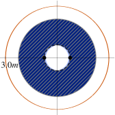
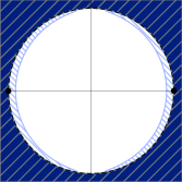
$a=\frac{2}{5}a_{\mathrm{max}}$
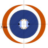
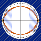
$a=\frac{4}{5}a_{\mathrm{max}}$
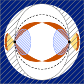
$a=a_{\mathrm{max}}$

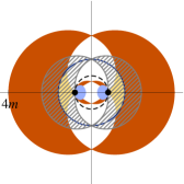
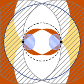
Figure 3: Photon regions in Kerr space-time for spins $a=\lambda a_{\mathrm{max}}$, where $a_{\mathrm{max}}=m$. The plots on the right show a magnified inner part.

$a=\frac{1}{50}a_{\mathrm{max}}$
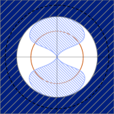
$a=\frac{2}{5}a_{\mathrm{max}}$
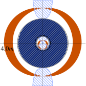
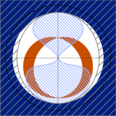
$a=\frac{4}{5}a_{\mathrm{max}}$
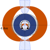
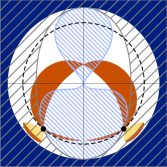
$a=a_{\mathrm{max}}$

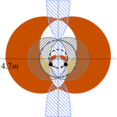
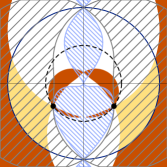
Figure 4: Photon regions in Kerr–NUT space-time with $\ell=\frac{3}{4}m$, $C=0$ for spins $a=\lambda a_{\mathrm{max}}$, where $a_{\mathrm{max}}=\sqrt{m^{2}+\ell^{2}}=\tfrac{5}{4}m$. The plots on the right show a magnified inner part.

$a=\frac{1}{50}a_{\mathrm{max}}$
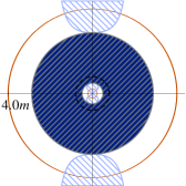
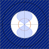
$a=\frac{2}{5}a_{\mathrm{max}}$
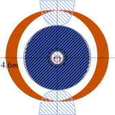
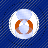
$a=\frac{4}{5}a_{\mathrm{max}}$
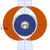
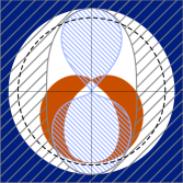
$a=a_{\mathrm{max}}$

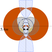
Figure 5: Photon regions in Kerr–Newman–NUT space-time ($\beta=\frac{5}{9}m^{2}$, $\ell=\frac{4}{3}m$, $C=0$) with a cosmological constant ($\Lambda={10}^{-2}m^{-2}$) for spins $a=\lambda a_{\mathrm{max}}$, where $a_{\mathrm{max}}\approx 1.51\,m$. The plots on the right show a magnified inner part.

$C=-2$	$C=-1$	$C=-\frac{1}{2}$	$C=0$	$C=\frac{1}{2}$	$C=1$	$C=2$

Figure 6: Photon regions for varying singularity parameter $C$ with fixed $a=\frac{4}{5}a_{\mathrm{max}}$, $\beta=\frac{5}{9}m^{2}$, $\ell=\frac{4}{3}m$, and $\Lambda=\bigl{\{}\begin{smallmatrix}{10}^{-2}m^{-2}&\text{for }C\leq 0\\ 0&\text{for }C>0\end{smallmatrix}\bigr{.}$, where $a_{\mathrm{max}}=\bigl{\{}\begin{smallmatrix}1.51m&\text{for }C\leq 0\\ 2\sqrt{5}\,m/3&\text{for }C>0\end{smallmatrix}\bigr{.}$. If existent, the cosmological horizon restricts the region ( ) where the causality is violated. If $C=1$ or $C=-1$, one of the two half-axes is regular and it is not surrounded by a causality violating region.

In the Kerr space-time, see Fig. 3, there is an exterior photon region at $r>r_{+}$ and an interior photon region at $r<r_{-}$. Both of them are symmetric with respect to the equatorial plane. Starting from the photon sphere at $r=3m$ for the non-rotating Schwarzschild case, the exterior photon region gets a crescent-shaped cross-section for $a\neq 0$ and grows with increasing spin $a$. The interior photon region consists of two connected components that are separated by the ring singularity. In the exterior photon region all spherical light orbits are unstable while in the interior photon region there are stable and unstable ones. Circular lightlike geodesics exist where the boundary of the photon region is tangent to a sphere $r=\mathrm{constant}$. We easily recognize the three well-known circular lightlike geodesics in the equatorial plane, but also two not-so-well-known cicular lightlike geodesics off the equatorial plane. The latter are situated in the region where $r<0$. The causality violating region is adjacent to the ring singularity and lies to the side of negative $r$. For small $a$, the ergoregion does not intersect the exterior photon region but for $a^{2}>m^{2}/2$ it does.

The additional gravitomagnetic charge $\ell$ of the Kerr–NUT space-time changes the symmetry behavior significantly, see Fig. 4. The plots are no longer symmetric with respect to the equatorial plane (but they remain, of course, axially symmetric). The exterior and interior photon regions show this asymmetry clearly. For a slowly rotating Kerr–NUT black hole, $a^{2}<\ell^{2}$, there is no ring singularity, and there are no stable spherical light rays. If the spin is increased, the ring singularity appears at $a^{2}=\ell^{2}$, degenerated to a point on the axis. With $a$ further increased, the ring singularity moves towards the equator and stable spherical light orbits come into existence between $r=0$ and $r=r_{-}$; as in the Kerr case, the interior photon region consists of two connected components that are separated by the ring singularity. While the ergosphere is not significantly affected by $\ell$, there is an additional causality violating region around the singularity on the axis which extends from the outer horizon at $r=r_{+}$ to $r=\infty$. The interior causality violating region is now extending from the inner horizon at $r=r_{-}$ to $r=-\infty$. The causality violating region depends on the Manko-Ruiz parameter $C$ which was chosen equal to zero in Fig. 4. (For other values of $C$ see Fig. 6.)

Adding an electric or magnetic charge parameter $\beta$ and a cosmological constant $\Lambda$ affects the photon regions little, see Fig. 5. The only qualitative effect of $\beta$ is in the fact that, in the case $a^{2}>\ell^{2}$, one of the two connected components of the interior photon region is now detached from the ring singularity. For non-zero $\Lambda$, higher spin values $a_{\mathrm{max}}$ are possible compared to space-times with $\Lambda=0$. For the pictures we have chosen a (small and) positive value for $\Lambda$ such that the domain of outer communication is bounded by a cosmological horizon. The latter is not shown in Fig. 5 because these pictures do not extend so far, but it is shown in Fig. 6. The cosmological horizon restricts the causality violating region which depends on the Manko-Ruiz parameter $C$, see Fig. 6.

IV Shadows of Black Holes

The existence of the photon region (16) around the black hole is essential for the construction of the shadow of a black hole. In the Introduction we have already explained how the shadow is constructed in the case of a Schwarzschild black hole. The same construction works, mutatis mutandis, in our more general black-hole space-times. We fix an observer in the domain of outer communication at Boyer-Lindquist coordinates $(r_{O},\vartheta_{O})$ and we think of light sources distributed on a sphere $r=r_{L}$ with some $r_{L}>r_{O}$.

For determining the shape of the shadow it is convenient to consider light rays which are sent from the observer’s position into the past. Then we can distinguish two types of orbits. Along light rays of the first type the radius coordinate reaches the value $r_{L}$, possibly after going through a local minimum, so that we can think of these light rays as being emitted from one of our light sources. Along light rays of the second type the radius coordinate decreases monotonically until it reaches the horizon at $r=r_{+}$, so these light rays cannot come from any of our light sources. Correspondingly, in the direction of light rays of the first type the observer would see brightness, and in the direction of light rays of the second type the observer would see darkness. The borderline case, i.e. the boundary of the shadow, corresponds to light rays that asymptotically spiral towards one of the unstable spherical light orbits in the exterior photon region which was discussed in Section III above. As in the Schwarzschild case, it is obvious from the geometry that the construction of the shadow works equally well if light sources are distributed, rather than on a sphere $r=r_{L}$ with $r_{L}>r_{O}$, anywhere else in the domain of outer communication except in the region filled by the above-mentioned light rays of the second type.

It is now our goal to calculate the boundary curve of the shadow on the observer’s sky. We consider an observer at position $(r_{O},\vartheta_{O})$ in the Boyer–Lindquist coordinates. (The $\varphi$ and $t$ coordinates of the observation event are irrelevant because of the symmetries of the metric.) We choose an orthonormal tetrad

$$e_{0} =\left.\frac{(\Sigma+a\chi)\partial_{t}+a\partial_{\varphi}}{\sqrt{\Sigma\Delta_{r}}}\right|_{(r_{O},\vartheta_{O})},$$ (19)

$$e_{1} =\left.\sqrt{\dfrac{\Delta_{\vartheta}}{\Sigma}}\,\partial_{\vartheta}\right|_{(r_{O},\vartheta_{O})},$$

$$e_{2} =\left.\frac{-(\partial_{\varphi}+\chi\partial_{t})}{\sqrt{\Sigma\Delta_{\vartheta}}\sin\vartheta}\right|_{(r_{O},\vartheta_{O})},$$

$$e_{3} =\left.-\sqrt{\frac{\Delta_{r}}{\Sigma}}\,\partial_{r}\right|_{(r_{O},\vartheta_{O})}.$$

at the observation event (see Fig. 7). We assume that the observer is in the domain of outer communication. This guarantees that $\Delta_{r}$ is positive, and so is $\Sigma$. Moreover, we assume that $\ell$ and $\Lambda$ are restricted by the inequality (7), which guarantees that $\Delta_{\vartheta}$ is positive. Hence, the coefficients in Eqs. (19) are indeed real and it is straight-forward to verify that $e_{0}$, $e_{1}$, $e_{2}$, $e_{3}$ are orthonormal. The timelike vector $e_{0}$ is to be interpreted as the four-velocity of our observer. The tetrad has been chosen such that $e_{0}\pm e_{3}$ are tangential to the principal null congruences of our metric. For an observer with four-velocity $e_{0}$ the vector $e_{3}$ gives the spatial direction towards the center of the black hole.

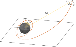
Figure 7: At an observation event with Boyer–Lindquist coordinates $(r_{O},\vartheta_{O})$ we choose an orthonormal tetrad $(e_{0},e_{1},e_{2},e_{3})$ according to Eqs. (19). For each light ray that is sent from the observation event into the past the tangent vector can be written as a linear combination of $e_{0}$, $e_{1}$, $e_{2}$ and $e_{3}$. In this way we can assign celestial coordinates to the direction of the tangent vector, see Fig. 8

For each light ray $\lambda(s)$ with coordinate representation $\bigl{(}r(s),\vartheta(s),\varphi(s),t(s)\bigr{)}$, we write the tangent vector as

$$\dot{\lambda}=\dot{r}\partial_{r}+\dot{\vartheta}\partial_{\vartheta}+\dot{\varphi}\partial_{\varphi}+\dot{t}\partial_{t}.$$ (20)

On the other hand, the tangent vector at the observation event can be written as

$$\dot{\lambda}=\alpha\big{(}-e_{0}+\sin\theta\cos\psi e_{1}+\sin\theta\sin\psi e_{2}+\cos\theta e_{3}\big{)}$$ (21)

where $\alpha$ is a scalar factor. From (10) and (11) we find that

$$\alpha=\left.g\big{(}\dot{\lambda},e_{0}\big{)}=\frac{aL_{z}-(\Sigma+a\chi)E}{\sqrt{\Sigma\Delta_{r}}}\right|_{(r_{O},\vartheta_{O})}.$$ (22)

Eq. (21) defines the celestial coordinates $\theta$ and $\psi$ for our observer, see Fig. 8. The direction towards the black hole corresponds to $\theta=0$.

Comparing coefficients of $\partial_{\varphi}$ and $\partial_{r}$ in (20) and (21) yields

$$\sin\psi =\left.\frac{\sqrt{\Delta_{\vartheta}}\sin\vartheta}{\sqrt{\Delta_{r}}\sin\theta}\left(\frac{\Sigma\Delta_{r}\dot{\varphi}}{(\Sigma+a\chi)E-aL_{z}}-a\right)\right|_{(r_{O},\vartheta_{O})},$$ (23)

$$\cos\theta =\left.\frac{\Sigma\dot{r}}{(\Sigma+a\chi)E-aL_{z}}\right|_{(r_{O},\vartheta_{O})}.$$

Upon substituting for $\dot{\varphi}$ and $\dot{r}$ from (12b) and (12d) we find from (23) that

$$\sin\psi =\left.\frac{\widetilde{L}_{E}+a\cos^{2}\vartheta+2\ell\cos\vartheta}{\sqrt{\Delta_{\vartheta}K_{E}}\sin\vartheta}\right|_{\vartheta=\vartheta_{O}},$$ (24)

$$\sin\theta =\left.\frac{\sqrt{\Delta_{r}K_{E}}}{r^{2}+\ell^{2}-a\widetilde{L}_{E}}\right|_{r=r_{O}},$$

where

$$\widetilde{L}_{E}=L_{E}-a+2\ell C.$$ (25)

The boundary curve of the shadow corresponds to light rays that asymptotically approach a spherical lightlike geodesic. Such a light ray must have the same constants of motion as the limiting spherical lightlike geodesic, i.e., by (15),

$$K_{E} =\left.\frac{16r^{2}\Delta_{r}}{(\Delta_{r}^{\prime})^{2}}\right|_{r=r_{p}},$$ (26)

$$a\widetilde{L}_{E} =\left.\Big{(}r^{2}+\ell^{2}-\frac{4r\Delta_{r}}{\Delta_{r}^{\prime}}\Big{)}\right|_{r=r_{p}},$$

where $r_{p}$ is the radius coordinate of the limiting spherical lightlike geodesic. Inserting the expressions for $K_{E}$ and $\widetilde{L}_{E}$ from (26) into (24) gives the boundary curve $\big{(}\psi(r_{p}),\theta(r_{p})\big{)}$ of the shadow.

We observe that the Manko-Ruiz parameter $C$ has no influence on the shadow and that the shadow is always symmetric with respect to a horizontal axis. The latter result follows from the fact that the points $(\psi,\theta)$ and $(\pi-\psi,\theta)$ correspond to the same constants of motion $K_{E}$ and $\widetilde{L}_{E}$. For $\ell\neq 0$ and $\vartheta_{O}\neq\pi/2$ this symmetry property was not to be expected.

For $a>0$, the $\theta$ coordinate takes its maximal value along the boundary curve at $\psi=-\pi/2$ and its minimal value at $\psi=\pi/2$. The corresponding values of the parameter $r_{p}$, which we denote by $r_{\mathrm{max}}(\vartheta_{O})$ and $r_{\mathrm{min}}(\vartheta_{O})$, respectively, can be determined by inserting (26) into (24) and equating $\psi$ to $\mp\pi/2$. We find that $r_{p}=r_{\mathrm{max/min}}(\vartheta_{O})$ is determined by the equation

$$\Big{(}\Sigma\Delta_{r}^{\prime}-4r\Delta_{r}\mp 4ar\sqrt{\Delta_{r}\Delta_{\vartheta}}\,\sin\vartheta\Big{)}\Big{|}_{(r=r_{p},\vartheta=\vartheta_{O})}=\,0\,.$$ (27)

Comparison with the inequality (16) shows that $r_{\mathrm{max}}(\vartheta_{O})$ and $r_{\mathrm{min}}(\vartheta_{O})$ are the radius values where the boundary of the exterior photon region intersects the cone $\vartheta=\vartheta_{O}$.

The case $a=0$ is special because then our method of parametrizing the boundary curve by $r_{p}$ does not work. If $a=0$ we have $r_{\mathrm{min}}(\vartheta_{O})=r_{p}=r_{\mathrm{max}}(\vartheta_{O})$, so (26) determines a unique value for $K_{E}$. Inserting this value into (24) gives the boundary curve of the shadow in the form $\big{(}\psi(\widetilde{L}_{E}),\theta(\widetilde{L}_{E})\big{)}$. We see that $\theta=\mathrm{constant}$ if $a=0$, i.e., that the shadow is circular.

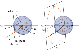
Figure 8: To each light ray at the observation event we assign celestial coordinates $\theta$ and $\psi$ with the help of Eq. (21), see figure on the left. The figure on the right shows the stereographic projection (red ball) of the point $(\theta,\psi)$ on the celestial sphere (black ball). The dotted (red) circles indicate the celestial equator $\theta=\pi/2$ and its projection.

Note that we have calculated the shadow for an observer with four-velocity $e_{0}$ according to (19). For an observer with a different four-velocity the shadow is distorted according to the standard aberration formula of special relativity.

In Figs. 9 and 10 we show pictures of the shadow, as it is seen by our chosen observer with four-velocity $e_{0}$. For calculating the boundary curve of the shadow we have used our analytical parameter representation, and for plotting it we have used stereographic projection from the celestial sphere onto a plane, as illustrated in Fig. 8. Standard Cartesian coordinates in this plane are given by

$$x(r_{p}) =-2\tan\Big{(}\frac{\theta(r_{p})}{2}\Big{)}\sin\big{(}\psi(r_{p})\big{)},$$ (28)

$$y(r_{p}) =-2\tan\Big{(}\frac{\theta(r_{p})}{2}\Big{)}\cos\big{(}\psi(r_{p})\big{)}.$$

In Fig. 9 the observer position is kept fixed at Boyer–Lindquist coordinates $r_{O}=5m$ and $\vartheta_{O}=\pi/2$. The parameters of the black hole are chosen such that the observer is always located in the domain of outer communication. Each of the five shadings corresponds to a certain choice of parameters $\beta$, $\ell$ and $\Lambda$, and for each choice the shadow is shown for four different values of the spin, $a=\lambda a_{\mathrm{max}}$, where $a_{\mathrm{max}}$ is determined by $\beta$, $\ell$ and $\Lambda$. The shadows of the first three cases—Kerr , Kerr–NUT , Kerr–Newman–NUT with cosmological constant —correspond to the photon regions presented in Figs. 3–5.

$a=\frac{2}{5}a_{\mathrm{max}}$	$a=\frac{4}{5}a_{\mathrm{max}}$
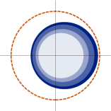
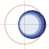
$a=\frac{1}{50}a_{\mathrm{max}}$	$a=a_{\mathrm{max}}$

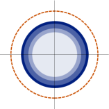
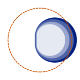
$\beta$	$0$	$0$	$\frac{5}{9}m^{2}$	$0$
$\ell$	$0$	$\frac{3}{4}m$	$\frac{4}{3}m$	$\frac{4}{3}m$
$\Lambda$	$0$	$0$	${10}^{-2}m^{-2}$	$0$
${a_{\mathrm{max}}}$	${m}$	${\frac{5}{4}m}$	${1.51m}$	${\frac{5}{3}m}$
	Kerr	Kerr–NUT	KN–NUT with $\Lambda$	Kerr–NUT

Figure 9: Shadow of a black hole for different parameters $a$, $\beta$, $\ell$ and $\Lambda$, seen by an observer at $r_{O}=5m$ and $\vartheta_{O}=\pi/2$. The cross hairs indicate the spatial direction towards the black hole, i.e., the spatial direction of the principal null congruences with respect to our observer with four-velocity $e_{0}$. The dashed (red) circle indicates the celestial equator, cf. Fig. 8.

We see that the shape of the shadow is largely determined by the spin $a$ of the black hole. With increasing $a$ the shadow becomes more and more asymmetric with respet to a vertical axis. This asymmetry is well-known from the Kerr metric and it is easily understood as a “dragging effect” of the rotating black hole on the light rays. The other parameters $\beta$, $\ell$ and $\Lambda$ have an effect on the size of the shadow but, at least for the naked eye, hardly on its shape. Note that the size of the shadow depends, of course, on $r_{O}$ and that there is no direct way of comparing radius coordinates in different space-times operationally. Therefore, if we want to get some information on the space-time from observing the shadow, the shape is much more relevant than the size.

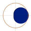
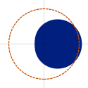
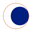
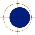
$\vartheta_{O}=\frac{\pi}{2}$	$\vartheta_{O}=\frac{3\pi}{8}$	$\vartheta_{O}=\frac{\pi}{4}$	$\vartheta_{O}=\frac{\pi}{8}$	$\vartheta_{O}=0$

Figure 10: Shadow of a black hole for an observer at $r_{O}=5m$ and different inclination angles $\vartheta_{O}$, with fixed $\beta=\frac{5}{9}m^{2}$, $\ell=\frac{4}{3}m$, $\Lambda={10}^{-2}m^{-2}$ and $a=a_{\mathrm{max}}\approx 1.51m$. As in Fig. 9, the cross hairs indicate the spatial direction towards the black hole and the dashed (red) circle indicates the celestial equator.

In Fig. 10 we consider an extremal black hole, $a=a_{\mathrm{max}}$, with fixed parameters $\beta$, $\ell$ and $\Lambda$. We keep the radius coordinate $r_{O}$ of the observer fixed, and we vary the inclination $\vartheta_{O}$. Clearly, the asymmetry with respect to the vertical axis vanishes if the observer approaches the axis, $\vartheta_{O}\to 0$. We have already emphasized the remarkable fact that there is no asymmetry with respect to the horizontal axis.

We should mention that in the case $\ell\neq 0$ some light rays have to pass through the singularity on the axis. We have assumed that these light rays are not blocked, i.e., that the source of the gravitomagnetic NUT field does not cast a shadow.

V Conclusions and Outlook

Based on a detailed analysis of the photon regions in black-hole space-times of the Plebański class, we have derived an analytical formula for the shadows of such black holes. As the space-times under consideration are not in general asymptotically flat and may have a cosmological horizon, one cannot restrict to observers at infinity as it was done in many earlier articles on shadows of black holes. Our formalism allows for observers at any Boyer–Lindquist coordinates in the domain of outer communication. The boundary curve of the shadow was calculated for observers with a certain four-velocity $e_{0}$, given by (19). For these observers, the shadow turned out to be always symmetric with respect to a horizontal axis, even for non-vanishing NUT parameter $\ell$ and for an observer off the equatorial plane. For observers with a four-velocity different from $e_{0}$, the shadow can be easily calculated by combining our results with the standard aberration formula of special relativity. If this additional aberration effect is taken into account, the boundary curve of the shadow will depend on the parameters $a$, $\ell$, $\beta$ and $\Lambda$, on the coordinates $r_{O}$ and $\vartheta_{O}$ of the observer, and on the velocity of the observer relative to an observer with four-velocity $e_{0}$. (The mass $m$ gives an overall scale, and the Manko-Ruiz parameter $C$ has no influence on the shadow.) We are planning to investigate, in a follow-up article, to what extent all these parameters can be determined from the boundary curve of the shadow. With an analytical formula for the boundary curve at hand, it is a natural idea to use a Fourier analysis of the boundary curve and to see how the parameters of the black hole can be extracted from the Fourier coefficients.

We have restricted to black-hole space-times, but a large part of the material presented in this paper is valid for naked singularities as well. In particular, the characterization of the photon region by inequality (16) is true in general. A major difference is in the fact that in the case of a naked singularity there is no domain of outer communication, so the possible observer positions are restricted only by a cosmological horizon, if present. The shadow of a naked singularity is drastically different from the shadow of a black hole, as was demonstrated by de Vries Vries.2000 for the Kerr-Newman case. While for a black hole the shadow is two-dimensional (an area on the sky, bounded by a closed curve), for a naked singularity the shadow is one-dimensional (an arc on the sky).

References

- (1) A. Eckart and R. Genzel, Nature 383, 415 (1996)
- (2) S. Gillessen et al., Astrophys. J. 692, 1075 (2009)
- (3) F. Eisenhauer et al., in Proceedings of the Workshop “Science with the VLT in the ELT Era”, Garching, 2009, edited by A. Moorwood (Springer, Netherlands, 2009), p. 361
- (4) S. S. Doeleman et al., Nature 455, 78 (2008)
- (5) J. L. Synge, Mon. Not. R. Astron. Soc. 131, 463 (1966)
- (6) A. M. Ghez et al., Astrophys. J. 689, 1044 (2008)
- (7) L. Huang, M. Cai, Zh.-Q. Shen, and F. Yuan, Month. Not. R. Astron. Soc. 379, 833 (2007)
- (8) J. M. Bardeen, in Black Holes (Les Astres Occlus), edited by C. DeWitt and B. S. DeWitt (Gordon and Breach, New York, 1973) p. 215
- (9) S. Chandrasekhar, The Mathematical Theory of Black Holes, (Oxford University Press, Oxford, 1983)
- (10) E. Teo, Gen. Relativ. Gravit. 35, 1909 (2003)
- (11) V. Perlick, Living Rev. Relativ. 7, 9 (2004)
- (12) A. de Vries, Class. Quantum Grav. 17, 123 (2000)
- (13) C. Bambi and N. Yoshida, Class. Quant. Grav. 27, 205006 (2010)
- (14) L. Amarilla, E. F. Eiroa, and G. Giribet, Phys. Rev. D 81, 124045 (2010)
- (15) L. Amarilla and E. F. Eiroa, Phys. Rev. D 85, 064019 (2012)
- (16) L. Amarilla and E. F. Eiroa, Phys. Rev. D 87, 044057 (2013)
- (17) A. Abdujabbarov, F. Atamurotov, Y. Kucukakça, B. Ahmedov, and U. Camci, Astrophys. Space Sci. 344, 429 (2012)
- (18) A. Yumoto, D. Nitta, T. Chiba, and N. Sugiyama, Phys. Rev. D 86, 103001 (2012)
- (19) Z. Li and C. Bambi, J. Cosmol. Astropart. Phys. 2014, 041 (2014)
- (20) K. Hioki and K.-I. Maeda, Phys. Rev. D 80, 024042 (2009)
- (21) T. Johannsen and D. Psaltis, Phys. Rev. D 83, 124015 (2011)
- (22) J. F. Plebański, Ann. Phys. 90, 196 (1975)
- (23) J. F. Plebański and M. Demiański, Ann. Phys. 98, 98 (1976)
- (24) H. Falcke, F. Melia, and E. Agol, Astrophys. J. 528, L13 (2000)
- (25) J. M. Bardeen and C. T. Cunningham, Astrophys. J. 183, 237 (1973)
- (26) J.-P. Luminet, Astron. Astrophys. 75, 228 (1979)
- (27) J. Dexter, E. Agol, P. C. Fragile, and J. C. McKinney, J. Phys.: Con. Ser. 372, 012023 (2012)
- (28) M. Mościbrodzka, H. Shiokawa, C. F. Gammie, and J. C. Dolence, Astrophys. J. Lett. 752, L1 (2012)
- (29) J. Dexter and P. C. Fragile, Mon. Not. R. Astron. Soc. 432, 2252 (2013)
- (30) B. Carter, Commun. Math. Phys. 10, 280 (1968)
- (31) J. G. Miller, J. Math. Phys. 14, 486 (1973)
- (32) J. B. Griffiths and J. Podolský, Exact Space-Times in Einstein’s General Relativity, (Cambridge University Press, Cambridge, 2009)
- (33) H. Stephani, D. Kramer, M. MacCallum, C. Hoenselaers, E. Herlt, Exact Solutions of Einstein’s Field Equations, (Cambridge University Press, Cambridge, 2003)
- (34) V. S. Manko and E. Ruiz, Class. Quantum Grav. 22, 3555 (2005)
- (35) A. N. Aliev and A. E. Gümrükçüoğlu, Phys. Rev. D 71, 104027 (2005)
- (36) V. Kagramanova, J. Kunz, E. Hackmann, and C. Lämmerzahl, Phys. Rev. D 81, 124044 (2010)
- (37) C. W. Misner, J. Math. Phys. 4, 924 (1963)
- (38) W. B. Bonnor, Math. Proc. Cambridge Philos. Soc. 66, 145 (1969)
- (39) E. Hackmann, V. Kagramanova, J. Kunz, and C. Lämmerzahl, Europhys. Lett. 88, 30008 (2009)
- (40) B. O’Neill, The Geometry of Kerr Black Holes (A K Peters, Wellesley, 1995)