Distributed Approximation Algorithms for Weighted Shortest Paths

A distributed network is modeled by a graph having $n$ nodes (processors) and diameter $D$. We study the time complexity of approximating weighted (undirected) shortest paths on distributed networks with a $O(\log n)$ bandwidth restriction on edges (the standard synchronous ${\sf CONGEST}$ model). The question whether approximation algorithms help speed up the shortest paths (more precisely distance computation) was raised since at least 2004 by Elkin (SIGACT News 2004). The unweighted case of this problem is well-understood while its weighted counterpart is fundamental problem in the area of distributed approximation algorithms and remains widely open. We present new algorithms for computing both single-source shortest paths (SSSP) and all-pairs shortest paths (APSP) in the weighted case.

Our main result is an algorithm for SSSP. Previous results are the classic $O(n)$-time Bellman-Ford algorithm and an $\tilde{O}(n^{1/2+1/2k}+D)$-time $(8k\lceil\log(k+1)\rceil-1)$-approximation algorithm, for any integer $k\geq 1$, which follows from the result of Lenzen and Patt-Shamir (STOC 2013). (Note that Lenzen and Patt-Shamir in fact solve a harder problem, and we use $\tilde{O}(\cdot)$ to hide the $O(\operatorname{poly}\log n)$ term.) We present an $\tilde{O}(n^{1/2}D^{1/4}+D)$-time $(1+o(1))$-approximation algorithm for SSSP. This algorithm is sublinear-time as long as $D$ is sublinear, thus yielding a sublinear-time algorithm with almost optimal solution. When $D$ is small, our running time matches the lower bound of $\tilde{\Omega}(n^{1/2}+D)$ by Das Sarma et al. (SICOMP 2012), which holds even when $D=\Theta(\log n)$, up to a $\operatorname{poly}\log n$ factor.

As a by-product of our technique, we obtain a simple $\tilde{O}(n)$-time $(1+o(1))$-approximation algorithm for APSP, improving the previous $\tilde{O}(n)$-time $O(1)$-approximation algorithm following from the results of Lenzen and Patt-Shamir. We also prove a matching lower bound. Our techniques also yield an $\tilde{O}(n^{1/2})$ time algorithm on fully-connected networks, which guarantees an exact solution for SSSP and a $(2+o(1))$-approximate solution for APSP. All our algorithms rely on two new simple tools: light-weight algorithm for bounded-hop SSSP and shortest-path diameter reduction via shortcuts. These tools might be of an independent interest and useful in designing other distributed algorithms.

1 Introduction

It is a fundamental issue to understand the possibilities and limitations of distributed/decentralized computation, i.e., to what degree local information is sufficient to solve global tasks. Many tasks can be solved entirely via local communication, for instance, how many friends of friends one has. Research in the last 30 years has shown that some classic combinatorial optimization problems such as matching, coloring, dominating set, or approximations thereof can be solved using small (i.e., polylogarithmic) local communication. However, many important optimization problems are “global” problems from the distributed computation point of view. To count the total number of nodes, to determining the diameter of the system, or to compute a spanning tree, information necessarily must travel to the farthest nodes in a system. If exchanging a message over a single edge costs one time unit, one needs $\Omega({\sf D})$ time units to compute the result, where ${\sf D}$ is the network’s diameter. In a model where message size could be unbounded (often known as the ${\sf LOCAL}$ model), one can simply collect all the information in $O({\sf D})$ time (ignoring time for the local computation), and then compute the result. A more realistic model, however, has to take into account the congestion issue and limits the size of a message allowed to be sent in a single communication round to some $B$ bits, where $B$ is typically set to $\log n$. This model is often called synchronous ${\sf CONGEST}$ (or ${\sf CONGEST}(B)$ if $B\neq\log n$). Time complexity in this model is one of the major studies in distributed computing [Pel00].

Many previous works in this model, including several previous FOCS/STOC papers (e.g. [GKP98, PR00, Elk06, DHK⁺12, LPS13]), concern graph problems. Here, we want to learn some topological properties of a network, such as minimum spanning tree (MST), minimum cut (mincut), and distances. These problems can be trivially solved in $O(m)$ rounds, where $m$ is the number of edges, by aggregating the whole network into one node. Of course, this is neither interesting nor satisfactory. The holy grail in the area of distributed graph algorithms is to beat this bound and, in many case, obtain a sublinear-time algorithm whose running time is in the form $\tilde{O}(n^{1-\epsilon}+{\sf D})$ for some constant $\epsilon>0$, where $n$ is the number of nodes and ${\sf D}$ is the network’s diameter. For example, through decades of extensive research, we now have an algorithm that can find an MST in $\tilde{O}(n^{1/2}+{\sf D})$ time [GKP98, KP98], and we know that this running time is tight [PR00]. This algorithm serves as a building block for several other sublinear-time algorithms (e.g. [Thu97, PT11, GK13, Nan14, Su14]).

It is also natural to ask whether we can further improve the running time of existing graph algorithms by mean of approximation, e.g., if we allow an algorithm to output a spanning tree that is almost, but not, minimum. This question has generated a research in the direction of distributed approximation algorithms which has become fruitful in the recent years. On the negative side, Das Sarma et al. [DHK⁺12] (building on [PR00, Elk06, KKP13]) show that MST and a dozen other problems, including mincut and computing the distance between two nodes, cannot be computed faster than $\tilde{O}(n^{1/2}+{\sf D})$ in the synchronous ${\sf CONGEST}$ model even when we allow a large approximation ratio. On the positive side, we start to be able to solve some problems in sublinear time by sacrifying a small approximation factor; e.g., we can $(1+\epsilon)$-approximate mincut in $\tilde{O}(n^{1/2}+{\sf D})$ time [Nan14, Su14] and $(3/2)$-approximate the network’s diameter in $O(n^{3/4}+{\sf D})$ time [HW12, PRT12]. The question whether distributed approximation algorithms can help improving the time complexity of computing shortest paths was raised a decade ago by Elkin [Elk04]. It is surprising that, despite so much progress on other problems in the last decade, the problem of computing shortest paths is still widely open, especially when we want a small approximation guarantee. Prior to our work, sublinear-time algorithms for computing single-source shortest path (SSSP) and linear-time algorithms for computing all-pairs shortest paths (APSP) have to pay a high approximation factor [LPS13]. This paper fills this gap with algorithms having small approximation guarantees.

1.1 The Model

Consider a network of processors modeled by an undirected unweighted $n$-node $m$-edge graph $G$, where nodes model the processors and edges model the bounded-bandwidth links between the processors. Let $V(G)$ and $E(G)$ denote the set of nodes and edges of $G$, respectively. The processors (henceforth, nodes) are assumed to have unique IDs in the range of $\{1,\ldots,\operatorname{poly}(n)\}$ and infinite computational power. Each node has limited topological knowledge; in particular, it only knows the IDs of its neighbors and knows no other topological information (e.g., whether its neighbors are linked by an edge or not). Nodes may also accept some additional inputs as specified by the problem at hand.

For the case of graph problems, the additional input is edge weights. Let $w:E(G)\rightarrow\{1,2,\ldots,\operatorname{poly}(n)\}$ be the edge weight assignment. We refer to network $G$ with weight assignment $w$ as the weighted network, denoted by $(G,w)$. The weight $w(uv)$ of each edge $uv$ is known only to $u$ and $v$. As commonly done in the literature (e.g., [KP08, LPSR09, KP98, GKP98, GK13]), we will assume that the maximum weight is $\operatorname{poly}(n)$; so, each edge weight can be sent through an edge (link) in one round.

There are several measures to analyze the performance of such algorithms, a fundamental one being the running time, defined as the worst-case number of rounds of distributed communication. At the beginning of each round, all nodes wake up simultaneously. Each node $u$ then sends an arbitrary message of $B=\log n$ bits through each edge $uv$, and the message will arrive at node $v$ at the end of the round.

We assume that nodes always know the number of the current round. To simplify notations, we will name nodes using their IDs, i.e. we let $V(G)\subseteq\{1,\ldots,\operatorname{poly}(n)\}$. Thus, we use $u\in V(G)$ to represent a node, as well as its ID. The running time is analyzed in terms of number of nodes $n$, number of edge $m$, and ${\sf D}$, the diameter of the network $G$. Since we can compute $n$ and $2$-approximate ${\sf D}$ in $O({\sf D})$ time, we will assume that every node knows $n$ and the $2$-approximate value of ${\sf D}$. We say that an event holds with high probability (w.h.p.) if it holds with probability at least $1-1/n^{c}$, where $c$ is an arbitrarily large constant.

1.2 Problems & Definitions

For any nodes $u$ and $v$, a $u$-$v$ path $P$ is a path $\langle u=x_{0},x_{1},\ldots,x_{\ell}=v\rangle$ where $x_{i}x_{i+1}\in E(G)$ for all $i$. For any weight assignment $w$, we define the weight or distance of $P$ as $w(P)=\sum_{i=0}^{\ell-1}w(x_{i}x_{i+1})$. Let $\mathcal{P}_{G}(u,v)$ denote the set of all $u$-$v$ paths in $G$. We use $\operatorname{\sf dist}_{G,w}(u,v)$ to denote the distance from $u$ to $v$ in $(G,w)$; i.e., $\operatorname{\sf dist}_{G,w}(u,v)=\min_{P\in\mathcal{P}_{G}(u,v)}w(P)$. We say that a path $P$ is a shortest $u$-$v$ path in $(G,w)$ if $w(P)=\operatorname{\sf dist}_{G,w}(u,v)$. The diameter of $(G,w)$ is $D(G,w)=\max_{u,v}\operatorname{\sf dist}_{G,w}(u,v)$. When we want to talk about the properties of the underlying undirected unweighted network $G$, we will drop $w$ from the notations. Thus, $\operatorname{\sf dist}_{G}(u,v)$ is the distance between $u$ and $v$ in $G$ and, ${\sf D}(G)$ is the diameter of $G$. We refer to ${\sf D}(G)$ by “hop diameter”, or sometimes simply “diameter”, and ${\sf D}(G,w)$ by “weighted diameter”. When it is clear from the context, we use ${\sf D}$ to denote ${\sf D}(G)$. We emphasize that, like other papers in the literature, the term ${\sf D}$ which appears in the running time of our algorithms is the diameter of the underlying unweighted network $G$.

Definition 1.1 (Single-Source and All-Pairs Shortest Paths (SSSP, APSP)).

In the single-source shortest paths problem (SSSP), we are given a weighted network $(G,w)$ as above and a source node $s$ (the ID of $s$ is known to every node). We want to find the distance between $s$ and every node $v$ in $(G,w)$, denoted by $\operatorname{\sf dist}_{G,w}(s,v)$. In particular, we want $v$ to know the value of $\operatorname{\sf dist}_{G,w}(s,v)$. In the all-pairs shortest paths problem (APSP), we want to find $\operatorname{\sf dist}_{G,w}(u,v)$ for every pair $(u,v)$ of nodes. In particular, we want both $u$ and $v$ to know the value of $\operatorname{\sf dist}_{G,w}(u,v)$.

For any $\alpha$, we say an algorithm $\mathcal{A}$ is an $\alpha$-approximation algorithm for SSSP if it outputs $\widetilde{\operatorname{\sf dist}}_{G,w}$ such that $\operatorname{\sf dist}_{G,w}(s,v)\leq\widetilde{\operatorname{\sf dist}}_{G,w}(s,v)\leq\alpha\operatorname{\sf dist}_{G,w}(s,v)$ for all $v$. Similarly, we say that $\mathcal{A}$ is an $\alpha$-approximation algorithm for APSP if it outputs $\widetilde{\operatorname{\sf dist}}_{G,w}$ such that $\operatorname{\sf dist}_{G,w}(u,v)\leq\widetilde{\operatorname{\sf dist}}_{G,w}(u,v)\leq\alpha\operatorname{\sf dist}_{G,w}(u,v)$ for all $u$ and $v$.

Remark

We emphasize that we do not require every node to know all distances. Also note that, while our paper focuses on computing distances between nodes, it can be used to find a routing path or compute a routing table as well. For example, after solving APSP, nodes can exchange all distance information with their neighbors in $O(n)$ time. Then, when a node $u$ wants to send a message to node $v$, it simply sends such message to the neighbor $x$ with smallest $\operatorname{\sf dist}_{G,w}(v,x)$. The name shortest paths is inherited from [DHK⁺12] (see the definition of shortest $s$-$t$ path problem in [DHK⁺12, Section 2.5]) and in particular the lower bound in [DHK⁺12] holds for our problem).

Problems	Topology	References	Time	Approximation
SSSP	General	Bellman&Ford [Bel58, For56]	$\tilde{O}(n)$	exact
		Lenzen&Patt-Shamir [LPS13]1.3	$\tilde{O}(n^{1/2+1/2k}+{\sf D})$	$8k\lceil\log(k+1)\rceil-1$
		this paper	$\tilde{O}(n^{1/2}{\sf D}^{1/4}+{\sf D})$	$1+o(1)$
			($=\tilde{O}(n^{3/4}+{\sf D})$)
	Fully-Connected	Baswana&Sen [BS07]	$\tilde{O}(n^{1/k})$	$2k-1$
		this paper	$\tilde{O}(n^{1/2})$	exact
APSP	General	Trivial	$O(m)$	exact
		Lenzen&Patt-Shamir [LPS13]	$\tilde{O}(n)$	$O(1)$
		this paper	$\tilde{O}(n)$	$1+o(1)$
	Fully-Connected	Baswana&Sen [BS07]	$\tilde{O}(n^{1/k})$	$2k-1$
		this paper	$\tilde{O}(n^{1/2})$	$2+o(1)$

Table 1: Summary of previous and our results (presented in Sections 1.4 and 1.3). Parameter $k\geq 1$ is an integer (note that the time complexities above are sublinear only when $k\geq 2$). Note that this table omits previous running times based on other parameters (such as shortest-path diameter).

1.3 Our Results

Our and previous results are summarized in Table 1 (see Section 1.4 for the details of previous results). As shown in the table, previous algorithms either have large approximation guarantee or large running time. In this paper, we aim at algorithms with both small approximation guarantees and small running time. We consider both SSSP and APSP and study algorithms on both general networks and fully-connected networks. Our main result is a sublinear-time $(1+o(1))$-approximation algorithm for SSSP on general graphs:

Theorem 1.2 (SSSP on general graph).

There is a distributed $(1+o(1))$-approximation algorithm that solves SSSP on any weighted $n$-node network $(G,w)$. It finishes in $\tilde{O}(n^{1/2}{\sf D}^{1/4}+{\sf D})$ time w.h.p.

For typical real-world networks (e.g., ad hoc networks and peer-to-peer networks) ${\sf D}$ is small (usually $\tilde{O}(1)$). (In some networks, an even stronger property also holds; e.g., a peer-to-peer network is usually assumed to be an expander [APRU12].) It is thus of a special interest to develop an algorithm in this setting. For example, [LPSP06] studied MST on constant-diameter networks. Das Sarma et al. [DNPT13] developed a $\tilde{O}((\ell{\sf D})^{1/2})$-time algorithm for computing a random walk of length $\ell$, which is faster than the trivial $O(\ell)$-time algorithm when ${\sf D}$ is small. In the same spirit, our algorithm is faster than previous algorithms. Moreover, in this case our running time matches the lower bound of $\tilde{\Omega}(n^{1/2}+{\sf D})$ [DHK⁺12, EKNP12], which holds even for any algorithm with $\operatorname{poly}(n)$ approximation ratio; thus, our result settles the status of SSSP for this case. Additionally, since the same lower bound also holds in the quantum setting [EKNP12], our result makes SSSP among a few problems (others are MST and mincut) that quantum communication cannot help speeding up distributed algorithms significantly.

Observe that our running time is sublinear as long as ${\sf D}$ is sublinear in $n$ (since $\tilde{O}(n^{1/2}{\sf D}^{1/4}+{\sf D})$ can be written as $\tilde{O}(n^{3/4}+{\sf D})$). As shown in Table 1, previously we can either solve SSSP exactly in $\tilde{O}(n)$ time using Bellman-Ford algorithm [Bel58, For56] or $(8k\lceil\log(k+1)\rceil-1)$-approximately, for any $k>1$, in $\tilde{O}(n^{1/2+1/2k}+{\sf D})$ time by applying the algorithm of Lenzen and Patt-Shamir [LPS13]${}^{\ref{christoph}}$. Our algorithm is the first that gives an output very close to the optimal solution in sublinear time. Our result also points to an interesting direction in proving a stronger lower bound for SSSP: in contrast to previous lower bound techniques which usually work on low-diameter networks, proving a stronger lower bound for SSSP needs a new technique that must exploit the fact that the network’s diameter is fairly large. As a by-product of our techniques, we also obtain a linear-time algorithm for APSP.

Theorem 1.3 (APSP on general graphs).

There is a distributed $(1+o(1))$-approximation algorithm that solves APSP on any weighted $n$-node network $(G,w)$ which finishes in $\tilde{O}(n)$ time w.h.p.

We also observe that this algorithm is essentially tight:

Observation 1.4 (Lower bound for APSP).

Any $\operatorname{poly}(n)$-approximation algorithm for APSP on an $n$-node weighted network $G$ requires $\Omega(\frac{n}{\log n})$ time. This lower bound holds even when the underlying network $G$ has diameter ${\sf D}(G)=2$. Moreover, for any $\alpha(n)=O(n)$, any $\alpha(n)$-approximation algorithm on an unweighted network requires $\Omega(\frac{n}{\alpha(n)\log n})$ time.

Observation 1.4 implies that the running time of our algorithm in Theorem 1.3 is tight up to a $\operatorname{poly}\log n$ factor, unless we allow a prohibitively large approximation factor of $\operatorname{poly}n$. Moreover, even when we restrict ourselves to unweighted networks, we still cannot significantly improve the running time, unless the approximation ratio is fairly large; e.g., any $n^{1-\delta}$-time algorithm must allow an approximation ratio of $\Omega(n^{\delta}/\log n)$. We note that a similar result to Observation 1.4 has been independently proved by Lenzen and Patt-Shamir [LPS13] in the context of name-independent routing scheme.

Other by-products of our techniques are efficient algorithms on fully-connected distributed networks, i.e., when $G$ is a complete graph. As mentioned earlier, it is of an interest to study algorithms on low-diameter networks. The case of fully-connected networks is an extreme case where ${\sf D}=1$. This special setting captures, e.g., overlay and peer-to-peer networks, and has received a considerable attention recently (e.g. [LPSPP05, LW11, PST11, Len13, DLP12, BHP12]). Obviously, this model gives more power to algorithms since every node can directly communicate with all other nodes; for example, MST can be constructed in $O(\log\log n)$ time [LPSPP05], as opposed to the $\tilde{\Omega}(n^{1/2}+{\sf D})$ lower bound on general networks. No sublinear-time algorithm for SSSP and APSP is known even on this model if we want an optimal or near-optimal solution. In this paper, we show such an algorithm. First, note that our $\tilde{O}(n^{1/2}{\sf D}^{1/4}+{\sf D})$-time algorithm in Theorem 1.2 already implies that SSSP can be $(1+o(1))$-approximated in $\tilde{O}(n^{1/2})$ time. We show that, as an application of our techniques for proving Theorem 1.2, we can get an exact algorithm within the same running time. More importantly, we show that these techniques, combined with some new ideas, lead to a $(2+o(1))$-approximation $\tilde{O}(\sqrt{n})$-time algorithm for APSP. The latter result is in contrast with the general setting where we show that a sublinear running time is impossible even when we allow large approximation ratios (Observation 1.4).

Theorem 1.5 (Sublinear time algorithm on fully-connected networks).

On any fully-connected weighted network, in $\tilde{O}(n^{1/2})$ time, SSSP can be solved exactly and APSP can be $(2+o(1))$-approximated w.h.p.

1.4 Related Work

Unweighted Case

SSSP and APSP are essentially well-understood in the unweighted case. SSSP can be trivially solved in $O({\sf D})$ time using a breadth-first search tree [Pel00, Lyn96]. Frischknecht, Holzer, and Wattenhofer [FHW12, HW12] show a (surprising) lower bound of $\Omega(n/\log n)$ for computing the diameter of unweighted networks, which implies a lower bound for solving unweighted APSP. This lower bound holds even for $(3/2-\epsilon)$-approximation algorithms. This lower bound is matched (up to a $\operatorname{poly}\log n$ factor) by $O(n)$-time deterministic exact algorithms for unweighted APSP found independently by [HW12] and [PRT12]. Another case that has been considered is when nodes can talk to any other node in one time unit. This can be thought of as a special case of APSP on fully-connected networks where edge weights are either $1$ or $\infty$. In this case, Holzer [Hol13] shows that SSSP can be solved in $\tilde{O}(n^{1/2})$ time.

Name-Dependent Routing Scheme

For the weighted SSSP and APSP on general networks, the best known results follow from the recent algorithm for computing tables for name-dependent routing and distance approximation by Lenzen and Patt-Shamir [LPS13]. In particular, consider any integer $k>1$. Lenzen and Patt-Shamir [LPS13, Theorem 4.12] showed that in time $\tau=\tilde{O}(n^{1/2+1/2k}+{\sf D})$ every node $u$ can compute a label $\lambda(u)$ of size $\sigma=O(\log(k+1)\log n)$ and a function $dist_{u}$ that maps label $\lambda(v)$ of any node $v$ to a distance approximation $dist_{u}(v)$ such that $\operatorname{\sf dist}_{G,w}(u,v)\leq dist_{u}(v)\leq\rho\operatorname{\sf dist}_{G,w}(u,v)$ where $\rho=8k\lceil\log(k+1)\rceil-1$. We can solve SSSP by running the above algorithm of Lenzen and Patt-Shamir and broadcasting the label $\lambda(s)$ of the source $s$ to all nodes. This takes time $\tau+\sigma=\tilde{O}(n^{1/2+1/2k}+{\sf D})$ and has an approximation guarantee of $\rho$. We can solve APSP by broadcasting $\lambda(v)$ for all $v$, taking time $\tau+n\sigma=\tilde{O}(n)$.

Sparsification

The shortest path problem is one of the main motivations to study distributed algorithms for graph sparsification. These algorithms have either super-linear time or large approximation guarantees. For example, Elkin and Zhang [EZ06] present an algorithm for the unweighted case based on a sparse spanner that takes (very roughly) $O(n^{\xi})$ time and gives $(1+\epsilon)$-approximate solution, for small constants $\xi$ and $\epsilon$. The algorithm is also extended to the weighted case but both running time and approximation guarantee are large (linear in terms of the largest edge weight). The running time could be traded-off with the approximation guarantee using, e.g., a $(2k-1)$-spanner of size $O(kn^{1+1/k})$ [BS07] where $k$ can vary; e.g., by setting $k=\log n/\log\log n$, we have an $O(n\log n)$-time $O(\log n/\log\log n)$-approximation algorithm (we need $O(k^{2})$ to construct a spanner and $O(kn^{1+1/k})=O(n\log n)$ to aggregate it). The spanner of [Pet10] can also be used to get a linear-time $(2^{O(\log^{*}{n})}\log n)$-approximation algorithm in the unweighted case.

In general, it is not clear how to use graph sparsification for computing shortest paths since we still need at least linear time to collect the sparse graph. However, it plays a crucial role in some previous algorithms, including the algorithm of Lenzen and Patt-Shamir [LPS13]. Moreover, by running the graph sparsification algorithm of Baswana and Sen [BS07] and collecting the network to one node, we can $(2k-1)$-approximate APSP in $O(kn^{1+1/k})$ time on general networks and $O(kn^{1/k})$ time on fully-connected networks, for any integer $k\geq 2$. This gives the fastest algorithm (with high approximation guarantees) on fully-connected networks.

Other Parameters

There are also some approximation algorithms whose running time is based on other parameters. These algorithms do not give any improvement for the worst values of their parameters. We do not consider these parameters in this paper since they are less standard. One important parameter is the shortest-path diameter, denoted by ${\sf SPDiam}(G,w)$. This parameter captures the number of edges in a shortest path between any pair of nodes (see Definition 3.8 for details). It naturally arises in the analysis of several algorithms. For example, Bellman-Ford algorithm [Bel58, For56] can be analyzed to have $O({\sf SPDiam}(G,w))$ time for SSSP. Khan et al. [KKM⁺12] gives a $\tilde{O}(n\cdot{\sf SPDiam}(G,w))$-time $O(\log n)$-approximation algorithm via metric tree embeddings [FRT04]. We can also construct Thorup-Zwick distance sketches [TZ05] of size $O(kn^{1/k})$ and stretch $2k-1$ in $\tilde{O}(kn^{1/k}\cdot{\sf SPDiam}(G,w))$ time [DDP12]. Since ${\sf SPDiam}(G,w)$ can be as large as $n$, these algorithms do not give any improvement to previous algorithms when analyzed in terms of $n$ and ${\sf D}$. One crucial component of our algorithms involves reducing the shortest-path diameter to be much less than $n$ (more in Section 2). Another shortest path algorithm with running time based on the network’s local path diameter is developed as a subroutine of the approximation algorithm for MST [KP08]. This algorithm solves a slightly different problem (in particular, nodes only have to know the distance to some nearby nodes) and cannot be used to solve SSSP and APSP.

Lower Bounds

The lower bound of Das Sarma et al. [DHK⁺12] (building on [Elk06, PR00, KKP13]) shows that solving SSSP requires $\tilde{\Omega}(\sqrt{n}+{\sf D})$ time, even when we allow $\operatorname{poly}(n)$ approximation ratio and the network has $O(\log n)$ diameter. This implies the same lower bound for APSP. Recently, [EKNP12] shows that the same $\tilde{\Omega}(\sqrt{n}+{\sf D})$ lower bound holds even in the quantum setting. These lower bounds are subsumed by Observation 1.4 for the case of APSP. Das Sarma et al. (building on [LPSP06]) also shows a polynomial lower bound on networks of diameter 3 and 4. It is still open whether there is a non-trivial lower bound on networks of diameter one and two [Elk04].

Other Works

While computing shortest paths is among the earliest studied problems in distributed computing, many classic works on this problem concern other objectives, such as the message complexity and convergence. When faced with the bandwidth constraint, the time complexities of these algorithms become higher than the trivial $O(m)$-time algorithm; e.g., Bellman-Ford algorithm and algorithms in [AR82, Hal97, AR93] require $\Omega(n^{2})$ time.

To the best of our knowledge, there is still no exact distributed algorithm for APSP that is faster than the trivial $O(m)$-time algorithm, except for the special case of BHC network, whose topology is structured as a balanced hierarchy of clusters. In this special case, the problem can be solved in $O(n\log n)$-time [AHT92]. For the related problem of computing network’s diameter and girth, many results are known in the unweighted case but none is previously known for the weighted case. Peleg, Roditty, and Tal [PRT12] shows that we can $\frac{3}{2}$-approximate the network’s diameter in $O(n^{1/2}{\sf D})$ time, in the unweighted case, and Holzer and Wattenhofer [HW12] presents an $O(\frac{n}{{\sf D}}+{\sf D})$-time $(1+\epsilon)$-approximation algorithm. By combining both algorithms, we get a $\frac{3}{2}$-approximation $O(n^{3/4}+{\sf D})$-time algorithm. In contrast, any $(\frac{3}{2}-\epsilon)$-approximation and $(2-\epsilon)$-approximation algorithm for computing the network’s diameter and girth requires $\Omega(n/\log n)$ time [HW12] and $\Omega(\sqrt{n}/\log n)$ time [FHW12], respectively. These bounds imply the same lower bound for approximation algorithms for APSP on unweighted networks. In particular, they imply that our approximation algorithms are tight, even on unweighted networks.

2 Overview

2.1 Tool 1: Light-Weight Bounded-Hop SSSP (Details in Section 3.1)

At the core of our algorithms is the light-weight $(1+o(1))$-approximation algorithm for computing bounded-hop distances. Informally, an $h$-hop path is a path containing at most $h$ edges. The $h$-hop distance between two nodes $u$ and $v$, denoted by $\operatorname{\sf dist}_{G,w}^{h}(u,v)$, is the minimum weight among all $h$-hop paths between $u$ and $v$. The $h$-hop SSSP problem is to find the $h$-hop distance between a given source node $s$ and all other nodes. This problem can be solved exactly in $O(h)$ time using the distributed version of Bellman-Ford algorithm. This algorithm is, however, not suitable for parallelization, i.e. when we want to solve $h$-hop SSSP from $k$ different sources. The reason is that Bellman-Ford algorithm is heavy-weight in the sense that they require so much communication between each neighboring nodes; in particular, this algorithm may require as many as $O(h)$ messages on each edge. Thus, running $k$ copies of this algorithm in parallel may require as many as $O(hk)$ messages on each edge, which will require $O(hk)$ time.

We show a simple algorithm that is not as accurate as Bellman-Ford algorithm but more suitable for parallelization: it can $(1+o(1))$-approximate $h$-hop SSSP in $\tilde{O}(h)$ time and is light-weight in the sense that every node sends a message (of size $O(\log n)$) to its neighbors only $\tilde{O}(1)$ times. Thus, when we run $k$ copies of this algorithm in parallel, we will require to send only $\tilde{O}(k)$ messages through each edge, which gives us a hope that we will require only additional $\tilde{O}(k)$ time. By a careful paralellization (based on the random delay technique of [LMR94]), we can solve $h$-hop SSSP from $k$ sources in $\tilde{O}(h+k)$ time. This is the first tool that we will use later.

Claim 2.1 (See Theorem 3.6 for a formal statement).

We can $(1+o(1))$-approximate $h$-hop SSSP from any $k$ nodes in $\tilde{O}(h+k)$ time.

The idea behind Claim 2.1 is actually very simple. Consider any path $P$ having at most $h$ hops. Let $\epsilon=1/\log n$ and $W^{\prime}=(1+\epsilon)^{i}$ where $i$ is such that $W^{\prime}\leq w(P)\leq(1+\epsilon)W^{\prime}$ (recall that $w(P)$ is the sum of weights of edges in $P$). Consider changing weight $w$ slightly to $w^{\prime}$ where $w^{\prime}(uv)=\lceil\frac{hw(uv)}{\epsilon W^{\prime}}\rceil$. Because $w^{\prime}(uv)-\frac{hw(uv)}{\epsilon W^{\prime}}\leq 1$, we have that

$$w(uv)\leq w^{\prime}(uv)\times\frac{\epsilon W^{\prime}}{h}\leq w(uv)+O(\epsilon)\frac{W^{\prime}}{h}.$$

It follows that

$$w(P)\leq w^{\prime}(P)\times\frac{\epsilon W^{\prime}}{h}\leq w(P)+O(\epsilon)W^{\prime}=(1+o(1))w(P).$$

In other words, it is sufficient for us to find $w^{\prime}(P)$. To this end, we observe that $w^{\prime}(P)=O(h/\epsilon)$. Thus, we can simply use the breadth-first search (BFS) algorithm [Pel00, Lyn96] on $(G,w^{\prime})$ for $O(h/\epsilon)$ rounds. The BFS algorithm is light-weight: it sends at most one message through each edge. Now to use this algorithm to solve $h$-hop SSSP, we have to try different values of $W^{\prime}$ in the form $(1+\epsilon)^{i}$. This makes our algorithm send $\tilde{O}(1)$ messages through each edge.

To the best of our knowledge, this simple technique has not been used before in the literature of distributed algorithms. In the dynamic data structure context, Bernstein has independently used a similar weight rounding technique to construct a bounded-hop data structure, which plays an important role in his recent breakthrough [Ber13]. Also, it was recently pointed out to us by a STOC 2014 reviewer that this technique is similar to the one used in the PRAM algorithm of Klein-Sairam [KS92] which was originally proposed for VLSI routing by Raghavan and Thomson [RT85]. The main difference between this and our weight approximation technique is that we always round edge weights up while the previous technique has to round the weights up and down randomly (with some appropriate probability). So, if we adopt the previous technique, then the approximation guarantee of our light-weight SSSP algorithm will hold only with high probability (in contrast, it always holds in this paper). More importantly, randomly rounding the weight could cause some edge to have a zero weight after rounding. This problem can be handled in the PRAM setting by contracting edges of weight zero. However, this will be a serious problem for us since we do not know how to handle zero edge weight.

2.2 Tool 2: Shortest-Path Diameter Reduction Using Shortcuts (Details in Section 3.2)

The other crucial idea that we need is the shortest-path diameter reduction technique. Recall that the shortest-path diameter of a weighted graph $(G,w)$, denoted by ${\sf SPDiam}(G,w)$, is the minimum number $h$ such that for any nodes $u$ and $v$, there is a shortest $u$-$v$ path in $(G,w)$ having at most $h$ edges; in other words, $\operatorname{\sf dist}_{G,w}^{h}(u,v)=\operatorname{\sf dist}_{G,w}(u,v)$ for all $u$ and $v$. As discussed in Section 1.4 there are algorithms that need $\tilde{O}({\sf SPDiam}(G,w))$ time to solve SSSP and APSP, e.g. Bellman-Ford algorithm. Thus, it is intuitively important to try to make the shortest-path diameter small. The second crucial tool of our algorithm is the following claim.

Claim 2.2 (See Theorem 3.10 for a formal statement).

If we add $k$ edges called shortcuts from every node $u$ to its $k$ nearest nodes (breaking tie arbitrarily), where for each such node $v$ the shortcut edge $uv$ has weight $\operatorname{\sf dist}_{G,w}(u,v)$, then we can bound the shortest-path diameter to $O(n/k)$.

We note that the above claim would be trivially true if we add a shortcut from every node to all nodes within $k$ hops from it. The non-trivial part is showing that it is sufficient to add shortcuts to only $k$ nearest nodes. Note that this claim holds only for undirected graphs and the proof has to carefully exploit the fact that the network is undirected.

To the best of our knowledge, there is no previous work that proves and uses this fact in the distributed setting. Previous work that is somewhat related is the BSP algorithm of Lenzen and Patt-Shamir [LPS13] which finds $h$-hop distances to $k$ nearest nodes in $O(hk)$ time. In this work, the algorithm is not used to create shortcuts, but rather to collect information about a sufficient number of nodes so that one of them is also in some set of uniformly sampled nodes. Another related work is the notion of $(d,\epsilon)$-hop set introduced by Cohen [Coh00] in the PRAM setting: our shortest path diameter reduction technique can be considered as a simple construction of $(d,0)$-hop set of size $O(n^{2}/d)$. It might be possible to improve our algorithm by applying a more advanced construction of such hop set to the distributed setting.

2.3 Sketches of Algorithms

APSP on General Networks (details in Section 4)

Algorithm for APSP follows almost immediately from the the first tool above. By applying Claim 2.1 with $h=k=n$, we can $(1+o(1))$-approximate SSSP with every node as a source in $\tilde{O}(n)$ time; in other words, we can $(1+o(1))$-approximate APSP in $\tilde{O}(n)$ time on general networks.

SSSP on Fully-Connected Networks (details in Section 5.1)

This result follows easily from the the second tool above. To compute SSSP exactly on fully-connected networks, we will compute $k$ shortcuts from every node, where $k=n^{1/2}$. To do this, we show that it is enough for every node to send $k$ lightest-weight edges incident to it to all other nodes (since running $k$ rounds of Dijkstra’s algorithm will only need these edges). This takes $O(n^{1/2})$ time. Using this information to modify the weight assignment from $w$ to $w^{\prime}$, we can reduce the shortest-path diameter of the network to ${\sf SPDiam}(G,w^{\prime})\leq\sqrt{n}$ without changing the distance between nodes; this fact is due to Claim 2.2. We then run Bellman-Ford algorithm on this $(G,w^{\prime})$ to solve SSSP; this takes ${\sf SPDiam}(G,w^{\prime})=O(n^{1/2})$ time.

APSP on Fully-Connected Networks (details in Section 5.2)

We will need both tools for this result. Step 1: Like the previous algorithm for SSSP on fully-connected network, we compute $n^{1/2}$ shortcuts from every node in $O(n^{1/2})$ time. Again, by Claim 2.2, this gives us a graph $(G,w^{\prime})$ such that ${\sf SPDiam}(G,w^{\prime})=O(n^{1/2})$. Additionally, every node sends these shortcuts to all other nodes (taking $O(n^{1/2})$ time). Step 2: We then randomly pick $n^{1/2}\operatorname{poly}\log n$ nodes and run the light-weight $h$-hop SSSP algorithm from these nodes, where $h={\sf SPDiam}(G,w^{\prime})=O(n^{1/2})$. By Claim 2.1, this takes $\tilde{O}(n^{1/2})$ time w.h.p. and gives us $(1+o(1))$-approximate values of the distances $\operatorname{\sf dist}_{G,w}(x,v)$ between each random node $x$ and all other nodes $v$ (known by $v$). Each node $v$ broadcasts distances to these $n^{1/2}\operatorname{poly}\log n$ random nodes to all other nodes, taking $\tilde{O}(n^{1/2})$ time.

After this, we show that every node can use the information they have received so far to compute $(2+o(1))$-approximate values of its distances to all other nodes. (In particular, every node uses the distances it receives to build a graph and uses the distances in such graph as approximate distances between itself and other nodes.) To explain the main idea, we show how to prove a $(3+o(1))$ approximation factor instead of $2+o(1)$: Consider any two nodes $u$ and $v$, and let $P$ be a shortest path between them. If $v$ is one of the $n^{1/2}$ nodes nearest to $u$, then $u$ already knows $\operatorname{\sf dist}_{G,w}(u,v)$ from the first step (when we compute shortcuts). Otherwise, by a standard hitting set argument, one of these $n^{1/2}$ nearest nodes must be picked as one of $n^{1/2}\operatorname{poly}\log n$ random nodes; let $x$ be such a node. Observe that $\operatorname{\sf dist}_{G,w}(u,x)\leq\operatorname{\sf dist}_{G,w}(u,v)$. By triangle inequality

$$\operatorname{\sf dist}_{G,w}(x,v)\leq\operatorname{\sf dist}_{G,w}(x,u)+\operatorname{\sf dist}_{G,w}(u,v)\leq 2\operatorname{\sf dist}_{G,w}(u,v).$$

Again, by triangle inequality,

$$\operatorname{\sf dist}_{G,w}(u,v)\leq\operatorname{\sf dist}_{G,w}(u,x)+\operatorname{\sf dist}_{G,w}(x,v)\leq 3\operatorname{\sf dist}_{G,w}(u,v);$$

in other words, $\operatorname{\sf dist}_{G,w}(u,x)+\operatorname{\sf dist}_{G,w}(x,v)$ is a $3$-approximate value of $\operatorname{\sf dist}_{G,w}(u,v)$. Note that $u$ knows the exact value of $\operatorname{\sf dist}_{G,w}(u,x)$ (from the first step) and the $(1+o(1))$-approximate value of $\operatorname{\sf dist}_{G,w}(x,v)$ (from the second step). So, it can compute a $(1+o(1))$-approximate value of $\operatorname{\sf dist}_{G,w}(u,x)+\operatorname{\sf dist}_{G,w}(x,v)$ which is a $(3+o(1))$-approximate value of $\operatorname{\sf dist}_{G,w}(u,v)$. Using the same argument, $v$ can also compute a $(3+o(1))$-approximate value of $\operatorname{\sf dist}_{G,w}(u,v)$. To extend this idea to a $(2+o(1))$-approximation algorithm, we use exactly the same algorithm but has to consider a few more cases.

SSSP on General Networks (details in Section 4)

Approximating SSSP in sublinear time needs both tools above and a few other ideas. First, we let $S$ be a set of $\frac{n^{1/2}}{{\sf D}^{1/4}}\operatorname{poly}\log n$ random nodes and the source $s$. We need the following.

Claim 2.3 (details in Section 4.1).

Let $h=n^{1/2}{\sf D}^{1/4}$. Every node $v$ can compute an approximate distance to $s$ if it knows (i) approximate $h$-hop distances between itself and all nodes in $S$, and (ii) distances between the source $s$ and all nodes in $S$ in the following weighted graph $(G^{\prime},w^{\prime})$: nodes in $G^{\prime}$ are those in $S$, and every edge $uv$ in $G^{\prime}$ has weight equal to the $h$-hop distance between $u$ and $v$ in $G$.

We call graph $(G^{\prime},w^{\prime})$ an overlay network since it can be viewed as a network sitting on the original network $(G,w)$. The idea of using the overlay network to compute distances is not new. It is a crucial tool in the context of dynamic data structures and distance oracle (e.g. [DFI05]). In distributed computing literature, it has appeared (in a slightly different form) in, e.g., [LPS13].

Our main task is now to achieve (i) and (ii) in Claim 2.3. Achieving (i) is in fact very easy: We simply run our light-weight $h$-hop SSSP from all nodes in $S$. By Claim 2.1, this takes time $\tilde{O}(|S|+h)=\tilde{O}(n^{1/2}{\sf D}^{1/4})$. In fact, by doing this we already partly achieve (ii): every node in $S$ already know the $h$-hop distance to all other nodes in $S$, thus it already has a “local” perspective in the overlay network $(G^{\prime},w^{\prime})$. To finish (ii), it is left to solve SSSP on $(G^{\prime},w^{\prime})$.

To do this, we will first reduce the shortest-path diameter of the overlay network $(G^{\prime},w^{\prime})$ by creating $k$ shortcuts, where $k={\sf D}^{1/2}$. As noted in the SSSP algorithm on fully-connected network, it is enough for every node in $(G^{\prime},w^{\prime})$ to send $k$ lightest-weight edges incident to it to all other nodes (since running $k$ rounds of Dijkstra’s algorithm will only need these edges). Broadcasting each such edge can be done in $O({\sf D})$ time via the breadth-first search tree, and broadcasting all $k|S|=\tilde{O}(n^{1/2}{\sf D}^{1/4})$ edges takes $\tilde{O}(n^{1/2}{\sf D}^{1/4}+{\sf D})$ time by pipelining. (See details in Section 4.2.) Let $(G^{\prime\prime},w^{\prime\prime})$ be an overlay network obtained from adding $k$ shortcuts to $(G^{\prime},w^{\prime})$. (As usual, nodes $u$ in $(G^{\prime\prime},w^{\prime\prime})$ only know weights $w^{\prime\prime}(uv)$ of edges $uv$ incident to it.) By Claim 2.2, ${\sf SPDiam}(G^{\prime\prime},w^{\prime\prime})=O(|S|/k)=\tilde{O}(n^{1/2}/{\sf D}^{3/4})$. Finally, we simulate our light-weight $h^{\prime}$-hop SSSP algorithm to solve SSSP from source $s$ on overlay $(G^{\prime\prime},w^{\prime\prime})$, where $h^{\prime}={\sf SPDiam}(G^{\prime\prime},w^{\prime\prime})=\tilde{O}(n^{1/2}/{\sf D}^{3/4})$. To do this efficiently, we need a slightly stronger property of our light-weight $h^{\prime}$-hop SSSP algorithm: recall that we have claimed that in our light-weight SSSP algorithm, each node sends a message through each edge only $\tilde{O}(1)$ times. In fact, we can show the following stronger claim.

Claim 2.4 (details in Theorem 3.2).

In the light-weight SSSP algorithm, each node communicates in each round by broadcasting the same message to its neighbors. Moreover, each node broadcasts messages only for $\tilde{O}(1)$ times.

The intuition behind the above claim is simple: at the heart of our light-weight SSSP algorithm, we solve $\tilde{O}(1)$ breadth-first search algorithms where, for each of these algorithms, each node broadcasts only once; it broadcasts its distance to the root, say $d$, at time $d$. Now we simulate our light-weight SSSP algorithm on $(G^{\prime\prime},w^{\prime\prime})$ as follows. When each node $v$ wants to broadcast a message to all its neighbors in $G^{\prime\prime}$, we broadcast this message to all nodes in $G$, using the breadth-first search tree of $G$ (see details in Section 4.3). This takes $O({\sf D})$ time. If we want to broadcast $M_{i}$ messages in a round $i$ of our light-weight SSSP algorithm, we can do so in $O({\sf D}+M_{i})$ time by pipelining. It can then be shown that the time we need to simulate all $r=\tilde{O}(h^{\prime})=\tilde{O}(n^{1/2}/{\sf D}^{3/4})$ rounds of our light-weight $h^{\prime}$-hop SSSP algorithm takes $\tilde{O}({\sf D}h^{\prime}+\sum_{i=1}^{r}M_{i})=\tilde{O}(n^{1/2}{\sf D}^{1/4}+{\sf D})$ (note that $\sum_{i=1}^{r}M_{i}=\tilde{O}(|S|)$ by Claim 2.4). (See details in Section 4.4.) This completes (ii) in Claim 2.3, and thus we can solve SSSP on $(G,w)$ in $\tilde{O}(n^{1/2}{\sf D}^{1/4}+{\sf D})$ time.

3 Main Tools

3.1 Light-Weight Bounded-Hop Single-Source and Multi-Source Shortest Paths

A key tool for our algorithm is a simple idea for computing a bounded-hop single-source shortest path and its extensions. Informally, an $h$-hop path is a path containing at most $h$ edges. The $h$-hop distance between two nodes $u$ and $v$ is the minimum weight among all $u$-$v$ $h$-hop paths. The problem of $h$-hop SSSP is to find the $h$-hop distance between a given source node $s$ and all other nodes. Formally:

Definition 3.1 ($h$-hop SSSP).

Consider any network $G$ with edge weight $w$ and integer $h$. For any nodes $u$ and $v$, let $\mathcal{P}^{h}(u,v)$ be a set of $u$-$v$ paths containing at most $h$ edges. We call $\mathcal{P}^{h}(u,v)$ a set of $h$-hop $u$-$v$ paths. Define the $h$-hop distance between $u$ and $v$ as

$$\operatorname{\sf dist}_{G,w}^{h}(u,v) =\begin{cases}\min_{P\in\mathcal{P}^{h}(u,v)}w(P)&\mbox{if $\mathcal{P}^{h}(u,v)\neq\emptyset$}\\ \infty&\mbox{otherwise.}\end{cases}$$

Let $h$-hop SSSP be the problem where, for a given weighted network $(G,w)$, source node $s$ (node $s$ knows that it is the source), and integer $h$ (known to every node), we want every node $u$ to know $\operatorname{\sf dist}_{G,w}^{h}(s,u)$.

This problem can be solved in $O(h+D)$ time using, e.g., the distributed version of Bellman-Ford’s algorithm. However, previous algorithms are “heavy-weight” in the sense that they require so much communication (i.e., there could be as large as $\Omega(h)$ messages sent through an edge) and thus are not suitable for parallelization. In this paper, we show a simple algorithm that can $(1+o(1))$-approximate $h$-hop SSSP in $\tilde{O}(h+D)$ time. Our algorithm is light-weight in the sense that every node broadcasts a message (of size $O(\operatorname{poly}\log n)$) to their neighbors only $O(\log n)$ times:

Theorem 3.2 (Light-weight $h$-hop SSSP algorithm; proof in Section 3.1.2).

There is an algorithm that solves $h$-hop SSSP on network $G$ with weight $w$ in $\tilde{O}(h+D)$-time and, during the whole computation, every node $u$ broadcasts $O(\log n)$ messages, each of size $O(\operatorname{poly}\log n)$, to its neighbors $v$.

Theorem 3.2, in its own form, cannot be directly used. We will extend it to an algorithm for computing $h$-hop multi-source shortest paths (MSSP). (Later, in Section 4.1 we will also extend this result to overlay networks.) The rest of this subsection is devoted to proving Theorem 3.2.

3.1.1 Reducing Bounded-Hop Distance by Approximating Weights

Theorem 3.3 (Reducing Bounded-Hop Distance by Approximating Weights).

Consider any $n$-node weighted graph $(G,w)$ and an integer $h$. Let $\epsilon=1/\log n$. For any $i$ and edge $xy$, let $D^{\prime}_{i}=2^{i}$ and $w^{\prime}_{i}(xy)=\lceil\frac{2hw(xy)}{\epsilon D^{\prime}_{i}}\rceil$. For any nodes $u$ and $v$, if we let

$$\widetilde{\operatorname{\sf dist}}^{h}_{G,w}(u,v)=\min\left\{\frac{\epsilon D^{\prime}_{i}}{2h}\times\operatorname{\sf dist}_{G,w^{\prime}_{i}}(u,v)\mid i:\ \operatorname{\sf dist}_{G,w^{\prime}_{i}}(u,v)\leq(1+2/\epsilon)h\right\},$$

then $\operatorname{\sf dist}^{h}_{G,w}(u,v)\leq\widetilde{\operatorname{\sf dist}}^{h}_{G,w}(u,v)\leq(1+\epsilon)\operatorname{\sf dist}^{h}_{G,w}(u,v)$.

Note that the min term in Theorem 3.3 is over all $i$ such that $\operatorname{\sf dist}_{G,w^{\prime}_{i}}(u,v)\leq(1+2/\epsilon)h$. The proof of Theorem 3.3 heavily relies on Lemma 3.4 below.

Lemma 3.4 (Key Lemma for Reducing Bounded-Hop Distance by Approximating Weights).

Consider any nodes $u$ and $v$. For any $i$, let $w_{i}$ and $D^{\prime}_{i}$ be as in Theorem 3.3. Then,

$$\frac{\epsilon D^{\prime}_{i}}{2h}\times\operatorname{\sf dist}_{G,w^{\prime}_{i}}(u,v)\geq\operatorname{\sf dist}^{h}_{G,w}(u,v).$$ (1)

Moreover, for $i^{*}$ such that $D^{\prime}_{i^{*}-1}\leq\operatorname{\sf dist}^{h}_{G,w}(u,v)\leq D^{\prime}_{i^{*}}$, we have that

$$\operatorname{\sf dist}_{G,w^{\prime}_{i^{*}}}(u,v) \leq(1+2/\epsilon)h~{}~{}\mbox{and}$$ (2)

$$\frac{\epsilon D_{i^{*}}}{2h}\times\operatorname{\sf dist}_{G,w^{\prime}_{i^{*}}}(u,v) \leq(1+\epsilon)\operatorname{\sf dist}^{h}_{G,w}(u,v).$$ (3)

Proof.

Let $P=\langle u=x_{0},x_{1},\ldots,x_{\ell}=v\rangle$ be any shortest $h$-hop path between $u$ and $v$ (thus $2^{i^{*}-1}\leq w(P)\leq 2^{i^{*}}$ and $\ell\leq h$). Then,

$$\operatorname{\sf dist}_{G,w^{\prime}_{i^{*}}}(u,v) =\sum_{j=0}^{\ell-1}\left\lceil\frac{2hw(x_{j}x_{j+1})}{\epsilon D^{\prime}_{i^{*}}}\right\rceil$$

$$\leq\frac{2h}{\epsilon D^{\prime}_{i^{*}}}\sum_{j=0}^{\ell-1}w(x_{j}x_{j+1})+\ell$$

$$\leq\frac{2h}{\epsilon D^{\prime}_{i^{*}}}\operatorname{\sf dist}^{h}_{G,w}(u,v)+h$$ (4)

$$\leq(1+2/\epsilon)h$$

where the last inequality is because $D^{\prime}_{i^{*}}\geq\operatorname{\sf dist}^{h}_{G,w}(u,v)$. This proves Equation 2. Using Equation 4, we also have that

$$\frac{\epsilon D^{\prime}_{i^{*}}}{2h}\times\operatorname{\sf dist}_{G,w^{\prime}_{i^{*}}}(u,v) \leq\frac{\epsilon D^{\prime}_{i^{*}}}{2h}\times\left(\frac{2h}{\epsilon D^{\prime}_{i^{*}}}\operatorname{\sf dist}^{h}_{G,w}(u,v)+h\right)$$

$$\leq\operatorname{\sf dist}^{h}_{G,w}(u,v)+\frac{\epsilon}{2}D^{\prime}_{i^{*}}$$

$$\leq(1+\epsilon)\operatorname{\sf dist}^{h}_{G,w}(u,v)$$

where the last inequality is because $D^{\prime}_{i^{*}}=2D^{\prime}_{i^{*}-1}\leq 2\operatorname{\sf dist}^{h}_{G,w}(u,v)$. This proves Equation 3. Finally, observe that for any $i$ and the path $P$ defined as before, we have

$$\operatorname{\sf dist}_{G,w^{\prime}_{i}}(u,v) \geq\sum_{j=0}^{\ell-1}\frac{2hw(x_{j}x_{j+1})}{\epsilon D^{\prime}_{i}}$$

$$=\frac{2h}{\epsilon D^{\prime}_{i}}\operatorname{\sf dist}^{h}_{G,w}(u,v)\,.$$

It follows that

$$\frac{\epsilon D^{\prime}_{i}}{2h}\times\operatorname{\sf dist}_{G,w^{\prime}_{i}}(u,v) \geq\frac{\epsilon D^{\prime}_{i}}{2h}\times\left(\frac{2h}{\epsilon D^{\prime}_{i}}\operatorname{\sf dist}^{h}_{G,w}(u,v)\right)$$

$$=\operatorname{\sf dist}^{h}_{G,w}(u,v)\,.$$

This proves Equation 1 and completes the proof of Lemma 3.4. ∎

Now we are ready to prove Theorem 3.3.

Proof of Theorem 3.3.

Note that

$$\tilde{d}^{h}_{G,w}(u,v) =\min\left\{\frac{\epsilon D^{\prime}_{i}}{2h}\times\operatorname{\sf dist}_{G,w^{\prime}_{i}}(u,v)\mid i:\ \operatorname{\sf dist}_{G,w^{\prime}_{i}}(u,v)\leq(1+2/\epsilon)h\right\}$$

$$\leq\frac{\epsilon D^{\prime}_{i^{*}}}{2h}\times\operatorname{\sf dist}_{G,w^{\prime}_{i^{*}}}(u,v)$$

$$\leq(1+\epsilon)\operatorname{\sf dist}^{h}_{G,w}(u,v)$$

where $i^{*}$ is as in Lemma 3.4, the second inequality is due to the fact that $\operatorname{\sf dist}_{G,w^{\prime}_{i^{*}}}(u,v)\leq(1+2/\epsilon)h$ as in Equation 2, and the third inequality follows from Equation 3. This proves the second inequality in Theorem 3.3. The first inequality of Theorem 3.3 simply follows from the fact that $\frac{\epsilon D^{\prime}_{i}}{2h}\times\operatorname{\sf dist}_{G,w^{\prime}_{i}}(u,v)\geq\operatorname{\sf dist}^{h}_{G,w}(u,v)$ for all $i$, by Equation 1. ∎

3.1.2 Algorithm for Bounded-Hop SSSP (Proof of Theorem 3.2)

We now show that we can solve $h$-hop SSSP in $\tilde{O}(h+D)$ time while each node broadcasts $O(\log n)$ messages of size $O(\log n)$, as claimed in Theorem 3.2. Our algorithm is outlined in Algorithm 1. Given a parameter $h$ (known to all nodes) and weighted network $(G,w)$, it computes $w_{i}$, for all $i$, as defined in Theorem 3.3; i.e., every node $u$ internally computes $w_{i}(u,v)$ for all neighbors $v$. Note that this step needs no communication. Next, in Line 4 of Algorithm 1, for each value of $i$, the algorithm executes an algorithm for the bounded-distance SSSP problem with parameter $(G,w,s,K)$, where $(1+2/\epsilon)h$, as outlined in Algorithm 2 (we will explain this algorithm next). At the end of the execution of Algorithm 2, every node $u$ knows $\operatorname{\sf dist}_{i}^{\prime}(s,u)$ such that $\operatorname{\sf dist}_{i}^{\prime}(s,u)=\operatorname{\sf dist}_{G,w_{i}}(s,u)$ if $\operatorname{\sf dist}_{G,w_{i}}(s,u)\leq K$ and $\operatorname{\sf dist}_{i}^{\prime}(s,u)=\infty$ otherwise. Finally, we set $\widetilde{\operatorname{\sf dist}}^{h}_{G,w_{i}}(s,u)=\min_{i}\operatorname{\sf dist}^{\prime}_{i}(s,u)$. By Theorem 3.3, we have that $\operatorname{\sf dist}^{h}_{G,w}(u,v)\leq\widetilde{\operatorname{\sf dist}}^{h}_{G,w}(u,v)\leq(1+\epsilon)\operatorname{\sf dist}^{h}_{G,w}(u,v)=(1+o(1))\operatorname{\sf dist}^{h}_{G,w}(u,v)$ as desired.

We now explain Algorithm 2 for solving the bounded-distance SSSP problem. It is a simple modification of a standard bread-first tree algorithm. It runs for $K$ rounds. In the initial round (Round $0$), the source node $s$ broadcasts a message $(s,0)$ to all its neighbors to start the algorithm. This message is to inform all its neighbors that its distance from the source (itself) is $0$. In general, we will make sure that every node $v$ whose distance to $s$ is $\operatorname{\sf dist}_{G,w}(s,u)=\ell$ will broadcast a message $(s,\ell)$ to its neighbor at Round $\ell$. Every time a node $u$ receives a message of the form $(s,\ell)$ from its neighbor $v$, it knows that $\operatorname{\sf dist}_{G,w}(s,v)=\ell$; so, $u$ updates its distance to the minimum between the current distance and $\ell+w(uv)$. It is easy to check that every node $u$ such that $\operatorname{\sf dist}_{G,w}(s,u)<K$ broadcasts its message to all neighbors once at Round $\ell=\operatorname{\sf dist}_{G,w}(s,u)$. The correctness of Algorithm 2 immediately follows. Moreover, since we execute Algorithm 2 for $O(\log n)$ different values of $i$ (since the maximum weight is $\operatorname{poly}(n)$), it follows that every node broadcasts a message to their neighbors $O(\log n)$ times. Theorem 3.2 follows.

Algorithm 1 Bounded-Hop SSSP $(G,w,s,h)$

Input: Weighted undirected graph $(G,w)$, source node $s$, and integer $h$.

Output: Every node $u$ knows the value of $\widetilde{\operatorname{\sf dist}}^{h}_{G,w_{i}}(s,u)$ such that $\operatorname{\sf dist}^{h}_{G,w}(s,u)\leq\widetilde{\operatorname{\sf dist}}^{h}_{G,w_{i}}(s,u)\leq(1+o(1))\operatorname{\sf dist}^{h}_{G,w_{i}}(s,u)$.

1:Let $\epsilon=1/\log n$. For any $i$ and edge $xy$, let $D^{\prime}_{i}=2^{i}$ and $w^{\prime}_{i}(xy)=\lceil\frac{2hw(xy)}{\epsilon D^{\prime}_{i}}\rceil$. Let $K=(1+2/\epsilon)h$.

2:Let $t$ be the time this algorithm starts. We can assume that all nodes know $t$.

3:for all i do

4:     Solve bounded-distance SSSP with parameters $(G,w_{i},s,K)$ using Algorithm 2. (This takes $\tilde{O}(K)=\tilde{O}(h)$ time.) Let $\operatorname{\sf dist}^{\prime}_{i}(s,u)$ be the distance returned to node $u$.

5:end for

6:Each node $u$ computes $\widetilde{\operatorname{\sf dist}}^{h}_{G,w_{i}}(s,u)=\min_{i}\operatorname{\sf dist}^{\prime}_{i}(s,u)$.

Algorithm 2 Bounded-Distance SSSP $(G,w,s,K)$

Input: Weighted undirected graph $(G,w)$, source node $s$, and integer $K$.

Output: Every node $u$ knows $\operatorname{\sf dist}^{\prime}_{G,w}(s,u)$ where $\operatorname{\sf dist}^{\prime}_{G,w}=\operatorname{\sf dist}_{G,w}(s,u)$ if $\operatorname{\sf dist}_{G,w}(s,u)\leq K$ and $\operatorname{\sf dist}^{\prime}_{G,w}=\infty$ otherwise.

1:Let $t$ be the time this algorithm starts. We can assume that all nodes know $t$.

2:Initially, every node $u$ sets $\operatorname{\sf dist}^{\prime}_{G,w}(s,u)=\infty$.

3:In the beginning of this algorithm (i.e., at time $t$) source node $s$ sends a message $(s,0)$ to itself.

4:if a node $u$ receives a message $(s,\ell)$ for some $\ell$ from node $v$, then

5:     if ($\ell+w(u,v)\leq K$) and ($\ell+w(u,v)<\operatorname{\sf dist}^{\prime}_{G}(s,u)$) then

6:         $u$ sets $\operatorname{\sf dist}^{\prime}_{G}(s,u)=\ell+w(u,v)$.

7:     end if

8:end if

9:For any $x\leq K$, at time $t+x$, every node $u$ such that $\operatorname{\sf dist}^{\prime}_{G}(s,u)=x$ broadcasts message $(s,x)$ to all its neighbors to announce that $\operatorname{\sf dist}^{\prime}_{G}(s,u)=x$.

3.1.3 Bounded-Hop Multi-Source Shortest Paths

The fact that our algorithm for the bounded-hop single-source shortest path problem in Theorem 3.2 is light-weight allows us to solve its multi-source version, where there are many sources in parallel. The problem of bounded-hop multi-source shortest path is as follows.

Definition 3.5 ($h$-hop $k$-source shortest paths).

Given a weighted network $(G,w)$, integer $h$ (known to every node), and sources $s_{1},\ldots,s_{k}$ (each node $s_{i}$ knows that it is a source), the goal of the $h$-hop $k$-source shortest paths problem is to make every node $u$ knows $\operatorname{\sf dist}_{G,w}^{h}(s_{i},u)$ for all $1\leq i\leq k$.

The main result of this section is an algorithm for solving this problem in $\tilde{O}(k+h+D)$ time, as follows.

Theorem 3.6 ($k$-source $h$-hop shortest path algorithm).

There is an algorithm that $(1+o(1))$-approximates the $h$-hop $k$-source shortest paths problem on weighted network $(G,w)$ in $\tilde{O}(k+h+D)$ time; i.e., at its termination every node $u$ knows $\operatorname{\sf dist}^{\prime}_{G,w}(s_{i},u)$ such that

$$\operatorname{\sf dist}_{G,w}^{h}(s_{i},u)\leq\operatorname{\sf dist}^{\prime}_{G,w}(s_{i},u)\leq(1+o(1))\operatorname{\sf dist}_{G,w}^{h}(s_{i},u)$$

for all sources $s_{i}$.

The algorithm is conceptually easy: we simply run the algorithm for bounded-hop single-source shortest path in Theorem 3.2 (i.e. Algorithm 1) from $k$ sources in parallel. Obviously, this algorithm needs at least $\tilde{\Omega}(h+D)$ time since this is the guarantee we can get for the case of single source. Moreover, it is possible that one need has to broadcast $O(\log n)$ messages for each execution of Algorithm 1, making a total of $O(k\log n)$ messages; this will require $\tilde{O}(k)$ time. So, the best running time we can hope for is $\tilde{O}(k+h+D)$. It is, however, not obvious to achieve this running time since one execution could delay other executions; i.e., it is possible that all executions of Algorithm 1 might want a node to send a message at the same time making some of them unable to proceed to the next round. We show that by simply adding a small delay to the starting time of each execution, it is unlikely that many executions will delay each other.

The algorithm is very simple: Instead of starting the execution of Algorithm 1 from different source nodes at the same time, each execution starts with a random delay randomly selected from integers from $0$ to $k\log n$. The algorithm is outlined in Algorithm 3.

Algorithm 3 Multi-Source Bounded-Hop Shortest Path $(G,w,\{s_{1},\ldots,s_{k}\},h)$

Input: Weighted undirected graph $(G,w)$, $k$ source nodes $s_{1},\ldots,s_{k}$, and integer $h$.

Output: Every node $u$ knows $\operatorname{\sf dist}^{h}_{G,w}(s_{i},u)$ for all $i$.

1:Let $r_{1},\ldots,r_{k}$ be a number selected uniformly at random from $[0,k\log n]$. We can assume that all nodes know $r_{i}$, for all $r_{i}$. This can be done by, e.g., broadcasting all $r_{i}$ to all nodes in $O(k+D)$ time.

2:Let $t$ be the time this algorithm starts. We can assume that all nodes know $t$.

3:At time $t+r_{i}$, execute the bounded-hop single-source shortest path algorithm (Algorithm 1) on $(G,w,s_{i},h)$.

4:If at any time, more than $\log n$ messages is sent through an edge, we say that the algorithm fails. (We show that the algorithm fails with probability $O(1/n^{2})$ in Lemma 3.7.)

The crucial thing is to show that many executions of Algorithm 1 launched by Algorithm 3 do not delay each other. In particular, that we show that at most $\log n$ messages will be sent through each edge in every round, with high probability (if this does not happen, we say that the algorithm fails). We prove this in Lemma 3.7 below. Our proof is simply an adaptation of the random delay technique for package scheduling [LMR94]. Lemma 3.7 immediately implies Theorem 3.6, since each execution, which start at time $\tilde{O}(k)$ will finish in $\tilde{O}(h+D)$ rounds without being delayed.

Lemma 3.7 (Congestion guaranteed by the random delay technique).

For any source $s_{i}$ and node $u$, let ${\mathcal{M}}_{i,u}$ be the set of messages broadcasted by $u$ during the execution of Algorithm 1 with parameter $(G,w,s_{i},h)$. Note that $|{\mathcal{M}}_{i,u}|\leq c\log n$ for some constant $c$, by Theorem 3.2. Then, the probability that, in Algorithm 3, there exists time $t$, node $u$, and a set ${\mathcal{M}}\subseteq\bigcup_{i}{\mathcal{M}}_{i,u}$ such that $|{\mathcal{M}}|\geq\log n$, and all messages in ${\mathcal{M}}$ are broadcasted by $u$ at time $t=O(k+h+D)$, is $O(1/n^{2})$.

Proof.

Fix any node $u$, time $t$, and set ${\mathcal{M}}$ as above. Observe that, for any $i$, the time that a message $M\in{\mathcal{M}}_{i,u}$, is broadcasted by $u$ is determined by the random delay $r_{i}$ – there is only one value of $r_{i}$ that makes $u$ broadcasts $M$ at time $t$. In other words, for fixed $u$, $t$, and message $M\in\bigcup_{i}{\mathcal{M}}_{i,u}$,

$$Pr[\mbox{$M$ is sent by $u$ at time $t$}]\leq\frac{1}{k\log n}.$$

It follows that for fixed $u$, $t$, and set of messages ${\mathcal{M}}$,

$$Pr[\mbox{all messages in ${\mathcal{M}}$ is sent by $u$ at time $t$}]\leq\left(\frac{1}{k\log n}\right)^{|{\mathcal{M}}|}.$$

Note that we can assume that $|{\mathcal{M}}\cap{\mathcal{M}}_{i,u}|\leq 1$ since, for an execution of Algorithm 1 on a source $s_{i}$, every node $u$ broadcasts at most one message per round. This implies that $|{\mathcal{M}}|\leq k$, and, for any $m\leq k$, the number of such set ${\mathcal{M}}$ of size exactly $m$ is at most $\binom{k}{m}(c\log n)^{m}$ since each set ${\mathcal{M}}$ can be constructed by picking $m$ different sets ${\mathcal{M}}_{i,u}$, and picking one message out of $c\log n$ messages from each ${\mathcal{M}}_{i,u}$. Thus, for fixed $u$ and $t$, the probability that there exists ${\mathcal{M}}$ such that $|{\mathcal{M}}|\geq\log n$ and all messages in ${\mathcal{M}}$ is sent by $u$ at time $t$ is at most

$$\sum_{m=\log n}^{k}\binom{k}{m}(c\log n)^{m}\left(\frac{1}{k\log n}\right)^{m}.$$

Using the fact that for any $0<b<a$, $\binom{a}{b}\leq(ae/b)^{b}$, the previous quantity is at most

$$\sum_{m=\log n}^{k}\left(\frac{ke}{m}\right)^{m}(c\log n)^{m}\left(\frac{1}{k\log n}\right)^{m} \leq\sum_{m=\log n}^{k}\left(\frac{ec}{m}\right)^{m}$$

$$\leq k\left(\frac{ec}{\log n}\right)^{\log n}.$$

For large enough $n$, the above quantity is at most $1/n^{4}$. We conclude that for fixed $u$ and $t$, the probability that there exists ${\mathcal{M}}$ such that $|{\mathcal{M}}|\geq\log n$ and all messages in ${\mathcal{M}}$ is sent by $u$ at time $t$ is at most $1/n^{4}$. By summing this probability over all nodes $u$ and $t=O(k+h+D)=O(n)$, Lemma 3.7 follows. ∎

3.2 Shortest-Path Diameter Reduction Using Shortcuts

In this section, we show a simple way to augment a graph with some edges (called “shortcuts”) to reduce the shortest-path diameter. The notion of shortest path diameter is defined as follows.

Definition 3.8 (Shortest-path distance and diameter).

For any weighted graph $(G,w)$, the shortest-path distance between any two nodes $u$ and $v$, denoted by ${\sf spdist}_{G,w}(u,v)$, is the minimum integer $h$ such that $\operatorname{\sf dist}_{G,w}^{h}(u,v)=\operatorname{\sf dist}_{G,w}(u,v)$. That is, it is the minimum number of edges among the shortest $u$-$v$ paths. The shortest-path diameter of $(G,w)$, denoted by ${\sf SPDiam}(G,w)$, is defined to be $\max_{u,v\in V(G)}{\sf spdist}_{G,w}(u,v)$. In other words, it is the minimum integer $h$ such that $\operatorname{\sf dist}_{G,w}^{h}(u,v)=\operatorname{\sf dist}_{G,w}(u,v)$ for all nodes $u$ and $v$.

Definition 3.9 ($k$-shortcut graph).

Consider any $n$-node weighted graph $(G,w)$ and an integer $k\neq n-1$. For any node $u$, let $S^{k}_{G,w}(u)\subseteq V(G)$ be the set of exactly $k$ nodes nearest to $u$ (excluding $u$); i.e. $u\notin S^{k}_{G,w}(u)$, $|S^{k}_{G,w}(u)|=k$, and for all $v\in S^{k}_{G,w}(u)$ and $v^{\prime}\notin S^{k}_{G,w}(u)$, $\operatorname{\sf dist}_{G,w}(u,v)\leq\operatorname{\sf dist}_{G,w}(u,v^{\prime})$. The $k$-shortcut graph of $(G,w)$, denoted by $(G,w)^{k}$, is a weighted graph resulting from adding an edge $uv$ of weight $\operatorname{\sf dist}_{G,w}(u,v)$ for every $u\in V(G)$ and $v\in S^{k}_{G,w}(u)$. When it is clear from the context, we will write $S^{k}(u)$ instead of $S^{k}_{G,w}(u)$.

Theorem 3.10 (Main result of Section 3.2: Reducing the shortest-path diameter by shortcuts).

For any $n$-node weighted undirected graph $(G,w)$ and integer $k$, if $(G^{\prime},w^{\prime})$ is the $k$-shortcut graph of $(G,w)$, then ${\sf SPDiam}(G^{\prime},w^{\prime})<4n/k$.

Proof.

Consider any nodes $u$ and $v$, and let

$$P=\langle u=x_{0},x_{1},\ldots,x_{\ell}=v\rangle$$

be the shortest $u$-$v$ path in $(G^{\prime},w^{\prime})$ with smallest number of edges; i.e. there is no path $Q$ in $(G^{\prime},w^{\prime})$ such that $|E(Q)|<|E(P)|$ and $w^{\prime}(Q)\leq w^{\prime}(P)$. For any node $x$, let $S^{k}(x)$ be the set of $k$ nodes nearest to $x$ in $(G,w)$, as in Definition 3.9. We claim that for any integer $0\leq i\leq(\ell/4)-1$, we have

$$S^{k}(x_{4i})\cap S^{k}(x_{4(i+1)})=\emptyset.$$

This claim immediately implies that $\ell<4n/k$, thus Theorem 3.10; otherwise, $|\bigcup_{0\leq i\leq\ell/4}S_{k}(x_{4i})|\geq(k+1)(n/k)>n$, which is impossible. It is thus left to prove the claim that $S^{k}(x_{4i})\cap S^{k}(x_{4(i+1)})=\emptyset$. Now, consider any $1\leq i\leq\ell/4$. Observe that

$$x_{4i+2}\notin S^{k}(x_{4i}).$$ (5)

Otherwise, $(G^{\prime},w^{\prime})$ will contain edge $x_{4i}x_{4i+2}$ of weight $\operatorname{\sf dist}_{G,w}(x_{4i},x_{4i+2})$. This implies that $P^{\prime}=\langle x_{0},\ldots,x_{4i-1},x_{4i},x_{4i+2},x_{4i+3},\ldots,x_{\ell}=v\rangle$ is a shortest $u$-$v$ path in $(G^{\prime},w^{\prime})$ containing $\ell-1$ edges, contradicting the fact that $P$ has the smallest number of edges among shortest $u$-$v$ paths in $(G^{\prime},w^{\prime})$. By the same argument, we have

$$x_{4i+2}\notin S^{k}(x_{4(i+1)}).$$ (6)

By the definition of $S^{k}$, Equations 5 and 6 imply that

$$\forall y\in S^{k}(x_{4i}) \operatorname{\sf dist}_{G,w}(x_{4i},y) \leq\operatorname{\sf dist}_{G,w}(x_{4i},x_{4i+2}),~{}~{}~{}\mbox{and}$$ (7)

$$\forall y\in S^{k}(x_{4(i+1)}) \operatorname{\sf dist}_{G,w}(x_{4(i+1)},y) \leq\operatorname{\sf dist}_{G,w}(x_{4(i+1)},x_{4i+2})$$ (8)

respectively. Now, assume for a contradiction that there is a node $y\in S^{k}(x_{4i})\cap S^{k}(x_{4(i+1)})$. Consider a path

$$P^{\prime\prime}=\langle x_{0},\ldots,x_{4i-1},x_{4i},y,x_{4(i+1)},x_{4(i+1)+1},\ldots,x_{\ell}=v\rangle.$$

Observe that $P^{\prime\prime}$ contains $\ell-3$ edges. Moreover, Equations 7 and 8 imply that

$$w^{\prime}(x_{4i}y) =\operatorname{\sf dist}_{G,w}(x_{4i},y)\leq\operatorname{\sf dist}_{G,w}(x_{4i},x_{4i+2})~{}~{}~{}\mbox{and}~{}~{}~{}$$

$$w^{\prime}(x_{4(i+1)}y) =\operatorname{\sf dist}_{G,w}(x_{4(i+1)},y)\leq\operatorname{\sf dist}_{G,w}(x_{4(i+1)},x_{4i+2})$$

which further imply that $w^{\prime}(P^{\prime\prime})\leq w^{\prime}(P)$. This means that $P^{\prime\prime}$ is a shortest $u$-$v$ paths in $(G^{\prime},w^{\prime})$ and contradicts the fact that $P$ has the smallest number of edges among shortest $u$-$v$ paths in $(G^{\prime},w^{\prime})$. Thus, $S^{k}(x_{4i})\cap S^{k}(x_{4(i+1)})=\emptyset$ as desired. ∎

We note a simple fact that will be used throughout this paper: we can compute $S^{k}_{G,w}(u)$ and $\operatorname{\sf dist}_{G,w}(u,v)$ for all $v\in S^{k}_{G,w}(u)$ if we know $k$ smallest edges incident to every nodes. The precise statement is as follows.

Definition 3.11 ($E^{k}(u)$ and $(G^{k},w)$).

For any node $u$, let $E^{k}(u)$ be the set of $k$ edges incident to $u$ with minimum weight (breaking tie arbitrarily); i.e., for every edge $uv\in E^{k}(u)$ and $uv^{\prime}\notin E^{k}(u)$, we have $w(uv)\leq w(uv^{\prime})$. Let $(G^{k},w)$ be the subgraph of $(G,w)$ whose edge set is $\bigcup_{v\in V(G)}E^{k}(v)$.

We note that for some graph $(G,w)$, the sets $E^{k}(u)$ and $S^{k}_{G,w}(u)$ might not be uniquely defined. To simplify our statement and proofs, we will assume that $(G,w)$ has the following property, which makes both $S^{k}_{G,w}(u)$ and $S^{k}_{G^{k},w}(u)$ unique: every edge $uv\in E(G)$ has a unique value of $w(uv)$, and every pair of nodes $u$ and $v$ has a unique value of $\operatorname{\sf dist}_{G,w}(u,v)$ and $\operatorname{\sf dist}_{G^{k},w}(u,v).$ Removing these assumptions can be easily done by breaking ties arbitrarily.

Observation 3.12 (Computing shortcut edges using $(G^{k},w)$).

For any node $u$,

• $S^{k}_{G,w}(u)=S^{k}_{G^{k},w}(u)$, and

• $\operatorname{\sf dist}_{G,w}(u,v)=\operatorname{\sf dist}_{G^{k},w}(u,v)$, for any $v\in S^{k}_{G,w}(u)$.

In other words, using only edges in $\bigcup_{v\in V(G)}E^{k}(v)$ and their weights, we can compute all $k$-shortcut edges.

Proof.

The intuition behind Observation 3.12 is that Dijkstra’s algorithm can be used to compute $S^{k}_{G,w}(u)$ and $\{\operatorname{\sf dist}_{G,w}(u,v)\}_{v\in S^{k}_{G,w}(u)}$ by executing it for $k$ iterations, and this process will never need any edge besides those in $(G^{k},w)$. Below we provide a formal proof that does not require the knowledge of Dijkstra’s algorithm.

Let $T_{u}$ be a shortest path tree rooted at $u$ in $(G,w)$. Assume for a contradiction that there is a node $v\in S^{k}_{G,w}(u)\setminus S^{k}_{G^{k},w}(u)$. Let $z$ be the parent of $v$ in $T_{u}$. The fact that $v\notin S^{k}_{G^{k},w}(u)$ implies that $zv\notin E^{k}(z)$; thus, there exists $v^{\prime}$ in $E^{k}(z)\setminus S^{k}_{G^{k},w}(u)$ (since $|E^{k}(z)|=|S^{k}_{G^{k},w}(u)|=k$ and $S^{k}_{G^{k},w}(u)\setminus E^{k}(z)\neq\emptyset$). Note that since $v\notin E^{k}(z)$, we have $w(zv^{\prime})<w(zv)$ (recall that we assume that edge weights are distinct). This, however, implies that

$$\operatorname{\sf dist}_{G,w}(u,v^{\prime})\leq\operatorname{\sf dist}_{G,w}(u,z)+w(zv^{\prime})<\operatorname{\sf dist}_{G,w}(u,v).$$

This contradicts the fact that $v\in S^{k}_{G,w}(u)$ and $v\notin S^{k}_{G,w}(u)$. ∎

4 Algorithms on General Networks

In this section, we present algorithms for SSSP and APSP on general distributed networks, as stated in Theorem 1.2 and Theorem 1.3. First, observe that APSP is simply a special case of the $h$-hop $k$-source shortest paths problem defined in Section 3.1.3 where we use $h=k=n$. Thus, by Theorem 3.6, there is an $(1+o(1))$-approximation algorithm that solves APSP in $\tilde{O}(k+h+D)=\tilde{O}(n)$ time with high probability. This immediately proves Theorem 1.3. The rest of this section is then devoted to showing a $\tilde{O}(n^{1/2}{\sf D}^{1/4}+{\sf D})$-time algorithm for SSSP as in Theorem 1.2, which require several non-trivial steps.

4.1 Reduction to Single-Source Shortest Path on Overlay Networks

In this section, we show that solving the single source shortest path problem on a network $(G,w)$ can be reduced to the same problem on a certain type of an overlay network, usually known as a landmark or skeleton (e.g. [Som12, LPS13]). In general, an overlay network $G^{\prime}$ is a virtual network of nodes and logical links that is built on top of an underlying real network $G$; i.e., $V(G^{\prime})\subset V(G)$ and an edge in $G^{\prime}$ (a “virtual edge”) corresponds to a path in $G$ (see, e.g., [EFK⁺12]). Its implementation is usually abstracted as a routing scheme that maps virtual edges to underlying routes. However, for the purpose of this paper, we do not need a routing scheme but will need the notion of hop-stretch which captures the number of hops in $G$ between two neighboring virtual nodes in $V(G^{\prime})$, as follows.

Definition 4.1 (Overlay network of hop-stretch $\lambda$).

Consider any network $G$. For any $\lambda$, a weighted network $(G^{\prime},w^{\prime})$ is said to be an overlay network of hop-stretch $\lambda$ embedded in $G$ if

1. $V(G^{\prime})\subseteq V(G)$,

2. $\operatorname{\sf dist}_{G}(u,v)\leq\lambda$ for every virtual edge $uv\in E(G^{\prime})$, and

3. for every virtual edge $uv\in E(G^{\prime})$, both $u$ and $v$ (as a node in $G$) knows the value of $w^{\prime}(uv)$.

We emphasize that $\lambda$ captures the number of hops ($\operatorname{\sf dist}_{G}(u,v)$) between two neighboring nodes $u$ and $v$, not the weighted distance ($\operatorname{\sf dist}_{G,w}(u,v)$). The main result of this section is an algorithm to construct an overlay network such that, if we can solve the single-source shortest path problem on such network, we can solve the single-source shortest path on the whole graph:

Theorem 4.2 (Main result of Section 4.1: Reduction to an overlay network).

For any weighted graph $(G,w)$, source node $s$, and integer $\alpha$, there is an $\tilde{O}(\alpha+n/\alpha+D)$-time distributed algorithm that embeds an overlay network $(G^{\prime},w^{\prime})$ in $G$ such that, with high probability,

1. $s\in V(G^{\prime})$,

2. $|V(G^{\prime})|=\tilde{O}(\alpha)$, and

3. if every node $u\in V(G)$ knows a $(1+o(1))$-approximate value of $\operatorname{\sf dist}_{G^{\prime},w^{\prime}}(s,v)$ for every node $v\in V(G^{\prime})$, then $u$ knows the $(1+o(1))$-approximate value of $\operatorname{\sf dist}_{G,w}(s,u)$.

Proof.

Our algorithm is as follows. First, every node $u$ selects itself to be in $V(G^{\prime})$ with probability $\alpha/n$. Additionally, we always keep source $s$ in $V(G^{\prime})$; this guarantees the first condition. Observe that $E[|V(G^{\prime})|]=1+(\alpha/n)\cdot(n-1)\leq 2\alpha$; so, by Chernoff’s bound (e.g. [MU05, Theorem 4.4]), $Pr[|(G^{\prime})|\geq 12\alpha\log n]\leq 1/n.$ This proves the second condition. To guarantee the last condition, we have to define edges and their weights in $G^{\prime}$. To do this, we invoke an algorithm for the bounded-hop multi-source shortest path problem in Theorem 3.6 (page 3.6), with nodes in $V(G^{\prime})$ as sources and $h=n\log n/\alpha$ hops. By Theorem 3.6, the algorithm takes $\tilde{O}(|V(G^{\prime})|+h+D)=\tilde{O}(\alpha+n/\alpha+D)$ time, and every node $u\in V(G)$ will know $\operatorname{\sf dist}^{\prime}_{G,w}(u,v)$ such that

$$\operatorname{\sf dist}_{G,w}^{h}(u,v)\leq\operatorname{\sf dist}^{\prime}_{G,w}(u,v)\leq(1+o(1))\operatorname{\sf dist}_{G,w}^{h}(u,v)$$

for all $v\in V(G^{\prime})$. For any $u,v\in V(G^{\prime})$ such that $\operatorname{\sf dist}^{\prime}_{G,w}(u,v)<\infty$, we add edge $uv$ with weight $w^{\prime}(u,v)=\operatorname{\sf dist}^{\prime}_{G,w}(u,v)$ to $G^{\prime}$. Note that both $u$ and $v$ knows the existence and weight of this edge. This completes the description of an overlay network $(G^{\prime},w^{\prime})$ embedded in $G$.

We are now ready to show the third condition, i.e., if a node $u\in V(G)$ knows a $(1+o(1))$-approximate value of $\operatorname{\sf dist}_{G^{\prime},w^{\prime}}(s,v)$ for all $v\in V(G^{\prime})$, then it knows a $(1+o(1))$-approximate value of $\operatorname{\sf dist}_{G,w}(s,u)$. Consider any node $u\in V(G)$, and let

$$P=\langle u=v_{0},v_{1},\ldots,v_{k}=s\rangle,$$

for some $k$, be a shortest path between $s$ and $u$ in $(G,w)$. Observe that if $k\leq n\log n/\alpha$, then $u$ knows $\operatorname{\sf dist}^{\prime}_{G,w}(u,v)$ which is a $(1+o(1))$-approximate value of $\operatorname{\sf dist}_{G,w}(s,u)$, and thus the third condition holds even when $u$ does not know a $(1+o(1))$-approximate value of $\operatorname{\sf dist}_{G^{\prime},w^{\prime}}(s,v)$ for any $v\in V(G^{\prime})$. It is thus left to consider the case where $k\geq n\log n/\alpha$. Let $i_{1}<i_{2}<\ldots<i_{t}$ be such that $v_{i_{1}},\ldots,v_{i_{t}}$ are nodes in $P\cap V(G^{\prime})$. Let $i_{0}=0$ (i.e., $v_{i_{0}}=u$). We note the following simple fact, which is very easy and well-known (e.g. [UY91]). We provide its proof here only for completeness.

Lemma 4.3 (Bound on the number of hops between two landmarks in a path).

For any $j$, $i_{j}-i_{j-1}\leq n\log n/\alpha$, with probability at least $1-2^{-\beta n}$, for some constant $\beta>0$ and sufficiently large $n$.

Proof.

We note a well-known fact that a set of random selected nodes $|V(G^{\prime})|$ of size $\alpha$ will “hit” a simple path of length at least $cn\log n/|V(G^{\prime})$, for some constant $c$, with high probability. To the best of our knowledge, this fact was first shown in [GK81] and has been used many times in dynamic graph algorithms (e.g. [DFI05] and references there in). The following fact appears as Theorem 36.5 in [DFI05] (attributed to [UY91]).

Fact 4.4 (Ullman and Yannakakis [UY91]).

Let $S\subseteq V(G)$ be a set of vertices chosen uniformly at random. Then the probability that a given simple path has a sequence of more than $(cn\log n)/|S|$ vertices, none of which are from $S$, for any $c>0$, is, for sufficiently large $n$, bounded by $2^{-\beta n}$ for some positive $\beta$.

Using $S=V(G^{\prime})$, which has size $\tilde{\Theta}(\alpha)$, we have that every subpath of $P$ of length at least $n\log n/\alpha$ contains a node in $V(G^{\prime})$, with high probability. The lemma follows by union bouding over the subpaths of $P$. This completes the proof of Lemma 4.3. ∎

It follows from the above lemma that $u$ knows $\operatorname{\sf dist}^{\prime}_{G,w}(u,v_{i_{1}})$ and, for any $j\geq 1$, $v_{i_{j}}v_{i_{j+1}}$ is an edge in the overlay network $G^{\prime}$ of weight $w^{\prime}(v_{i_{j}}v_{i_{j+1}})=\operatorname{\sf dist}^{\prime}_{G,w}(v_{i_{j}},v_{i_{j+1}})$, with probability at least $1-2^{-\beta n}$. Thus, with high probability,

$$\operatorname{\sf dist}_{G^{\prime},w^{\prime}}(v_{i_{1}},s)\leq\sum_{j=1}^{k-1}\operatorname{\sf dist}^{\prime}_{G,w}(v_{i_{j}},v_{i_{j+1}}).$$

Since $u$ already knows $\operatorname{\sf dist}^{\prime}_{G,w}(u,v_{i_{1}})$, it can now compute

$$\operatorname{\sf dist}^{\prime}_{G,w}(u,v_{i_{1}})+\sum_{j=1}^{k-1}\operatorname{\sf dist}^{\prime}_{G,w}(v_{i_{j}},v_{i_{j+1}})$$

which is at least $\operatorname{\sf dist}_{G,w}(u,s)$ and at most $(1+o(1))\operatorname{\sf dist}_{G,w}(u,s)$. We note one detail that, in fact, $u$ does not known which node is $v_{1}$, so it has to use the value of

$$\min_{v\in V(G^{\prime})}\operatorname{\sf dist}^{\prime}_{G,w}(u,v)+\operatorname{\sf dist}_{G^{\prime},w^{\prime}}(v,s)$$

as an estimate. By union bounding over all nodes $u$, Theorem 4.2 follows. ∎

4.2 Reducing the Shortest Path Diameter of Overlay Network $(G^{\prime},w^{\prime})$

In this section, we assume that we are given an overlay network $(G^{\prime},w^{\prime})$ embedded in the original network $(G,w)$, as show in Theorem 4.2. Our goal is to solve the single-source shortest path problem on $(G^{\prime},w^{\prime})$. Recall that $(G^{\prime},w^{\prime})$ has $|V(G^{\prime})|=\tilde{O}(\alpha)$ nodes, for some parameter $\alpha$, which will be fixed later. Note that the shortest path diameter (${\sf SPDiam}(G,w)$) of $(G^{\prime},w^{\prime})$ might be as large as $|V(G^{\prime})|=\tilde{O}(\alpha)$. Since the running time of our algorithm for single-source shortest path will depend on the shortest path diameter, we wish to reduce the shortest path diameter. We will apply the technique from Section 3.2 to do this task, as follows.

Theorem 4.5 (${\sf SPDiam}$ reduction of an overlay network).

For any parameter $\alpha$ and $\beta$, consider an overlay network $(G^{\prime},w^{\prime})$ of $\tilde{O}(\alpha)$ nodes, embedded in network $(G,w)$. There is a distributed algorithm that terminates in $\tilde{O}(\alpha\beta+{\sf D}(G))$ time and gives an overlay network $(G^{\prime\prime},w^{\prime\prime})$ such that $V(G^{\prime})=V(G^{\prime\prime})$, ${\sf SPDiam}(G^{\prime\prime},w^{\prime\prime})=\tilde{O}(\alpha/\beta)$, and for any nodes $u$ and $v$, $\operatorname{\sf dist}_{G^{\prime\prime},w^{\prime\prime}}(u,v)=\operatorname{\sf dist}_{G^{\prime},w^{\prime}}(u,v)$.

Proof.

Consider the following algorithm. First, every node in the overlay network $(G^{\prime},w^{\prime})$ broadcasts to all other nodes the values of $\beta$ edges incident to it with smallest weights (breaking ties arbitrarily). This step takes $\tilde{O}(\alpha\beta)$ time since there are $\alpha\beta$ edges broadcasted. Using these broadcasted edges, every node $v$ can compute $\beta$ nodes nearest to it (since any shortest path algorithm – Disjkstra’s algorithm for example – will only need to know $\beta$ smallest-weight edges to compute $\beta$ nearest nodes). Thus, $v$ can add $\beta$ shortcuts to the network $(G^{\prime},w^{\prime})$ to construct network $(G^{\prime\prime},w^{\prime\prime})$. In fact, the added shortcuts could be broadcasted to all nodes in $\tilde{O}(\alpha\beta+{\sf D}(G))$ time since each node will broadcast only $\beta$ shortcuts. This implies that we can build an overlay network $(G^{\prime\prime},w^{\prime\prime})$ in $\tilde{O}(\alpha\beta)$ time and, by Theorem 3.10, the shortest-path diameter of $(G^{\prime\prime},w^{\prime\prime})$ is ${\sf SPDiam}(G^{\prime\prime},w^{\prime\prime})=\tilde{O}(\alpha/\beta).$ ∎

4.3 Computing SSSP on Overlay Network $(G^{\prime\prime},w^{\prime\prime})$

In the final step of our sublinear-time SSSP algorithm, we solve SSSP on overlay network $(G^{\prime\prime},w^{\prime\prime})$ embedded in $(G,w)$ obtained in the previous section. Recall that for parameters $\alpha$ and $\beta$ which will be fixed later, $|V(G^{\prime\prime})|=\tilde{\Theta}(\alpha)$ and ${\sf SPDiam}(G^{\prime\prime},w^{\prime\prime})=\tilde{O}(\alpha/\beta)$.

Lemma 4.6 ($(1+o(1))$-approximate SSSP on $(G^{\prime\prime},w^{\prime\prime})$).

We can $(1+o(1))$-approximate SSSP on $(G^{\prime\prime},w^{\prime\prime})$ in $\tilde{O}({\sf D}(G)\alpha/\beta+\alpha)$ time.

Proof.

We will simulate the light-weight $h$-hop SSSP algorithm in Theorem 3.2 on the overlay network $(G^{\prime\prime},w^{\prime\prime})$ by using $h={\sf SPDiam}(G^{\prime\prime},w^{\prime\prime})=\tilde{O}(\alpha/\beta)$. To simulate this algorithm, we will view $(G^{\prime\prime},w^{\prime\prime})$ as a fully-connected overlay network where every node can communicate with other nodes by broadcasting, i.e. sending a message to every node in the original network $G$, which takes $O({\sf D}(G))$ time. In particular, every node in $(G^{\prime\prime},w^{\prime\prime})$ will simulate each round of this algorithm and wait until the messages that are sent in such round by all nodes are received by all nodes before starting the next round (see Algorithm 1).

Algorithm 1 Similating a broadcasting algorithm on an overlay network $(G^{\prime\prime},w^{\prime\prime})$

Input: An overlay network $(G^{\prime\prime},w^{\prime\prime})$ embedded on network $G$ and an algorithm $\mathcal{A}$ such that nodes communicate only by broadcasting a message to all its neighbors.

Goal: Simulate $\mathcal{A}$ on $(G^{\prime\prime},w^{\prime\prime})$ when we view $G^{\prime\prime}$ as a fully-connected overlay network.

1:for each round $i$ of algorithm $\mathcal{A}$ do

2:     Count the number of nodes in $G^{\prime\prime}$ that want to broadcast a message in this round of $\mathcal{A}$. Let $M_{i}$ be such number. Make every node in $G$ knows $M_{i}$. (This step takes $O({\sf D}(G))$ time.)

3:     Every node in $G^{\prime\prime}$ that wants to send a message broadcasts such message to every node in $G$. Wait for ${\sf D}(G)+M_{i}$ rounds to make sure that every node receives all $M_{i}$ messages before proceeding to round $i+1$.

4:end for

Simulating each round $i$ of this algorithm will take $\tilde{O}({\sf D}(G)+M_{i})$, where $M_{i}$ is the total number of messages broadcasted by all nodes in round $i$. This is because broadcasting $M_{i}$ messages to all nodes in the network (not just all neighbors) takes $\tilde{O}({\sf D}(G)+M_{i})$ time. Note that, by Theorem 3.2, this algorithm finishes in $\tilde{O}(h)$ rounds; thus, the total time needed to simulate this algorithm is $\tilde{O}(h{\sf D}(G)+M)$ where $M$ is the total number of messages broadcasted by all nodes throughout the algorithm. Since this algorithm is light-weight, every node in $G^{\prime\prime}$ broadcasts only $O(\log n)$ messages, and thus we can bound $M$ by $\tilde{O}(|V(G^{\prime\prime})|)=\tilde{O}(\alpha)$. So, the total running time is $\tilde{O}(h{\sf D}(G)+\alpha)=\tilde{O}({\sf D}(G)\alpha/\beta+\alpha)$ as claimed. ∎

4.4 Putting Everything Together (Proof of Theorem 1.2)

By Lemma 4.6, we can $(1+o(1))$-approximate SSSP on $(G^{\prime\prime},w^{\prime\prime})$ which, in turn, $(1+o(1))$-approximates SSSP on $(G^{\prime},w^{\prime})$, by Theorem 4.5. Then, by Theorem 4.2, we know that we can $(1+o(1))$-approximate SSSP on the original network $(G,w)$ as desired. We now analyze the running time. Constructing $(G^{\prime},w^{\prime})$ takes $\tilde{O}(\alpha+n/\alpha+{\sf D}(G))$, as in Theorem 4.2. Adding shortcuts to $(G^{\prime},w^{\prime})$ to construct $(G^{\prime\prime},w^{\prime\prime})$ takes $\tilde{O}(\alpha\beta+{\sf D}(G))$, by Theorem 4.5. Finally, solving SSSP on $(G^{\prime\prime},w^{\prime\prime})$ takes $\tilde{O}({\sf D}(G)\alpha/\beta+\alpha)$ by Lemma 4.6. So, the total running time of our algorithm is

$$\tilde{O}(n/\alpha+{\sf D}(G)+\alpha\beta+{\sf D}(G)\alpha/\beta).$$

By setting $\alpha=n^{1/2}/({\sf D}(G))^{1/4}$ and $\beta=({\sf D}(G))^{1/2}$, we get the running time of $\tilde{O}(n^{1/2}({\sf D}(G))^{1/4}+{\sf D}(G))$ as desired. Note that it is possible that $\beta\geq\alpha$. In this case, we will simply set $\beta=\alpha$ to get the claimed running time; in fact, this happens only when ${\sf D}(G)\geq n^{2/3}$, and the running time will be $\tilde{O}({\sf D}(G))$ in this case.

5 Algorithms on Fully-Connected Networks

5.1 $\tilde{O}(\sqrt{n})$-time Exact Algorithm for SSSP

In this section, we present an algorithm that solves SSSP exactly in $\tilde{O}(\sqrt{n})$ time on fully-connected networks. The algorithm has two simple phases, as shown in Algorithm 1. In the first phase, it reduces the shortest-path diameter using the techniques developed in Section 3.2. In particular, every node $u$ broadcasts $k=\sqrt{n}$ edges of smallest weight. Then, every node uses the information it receives to compute a $k$-shortcut graph $(G,w^{\prime})$, which can be done due to Observation 3.12. By Theorem 3.10, we have

$${\sf SPDiam}(G,w^{\prime})<4\sqrt{n}~{}~{}~{}\mbox{and}~{}~{}~{}\forall u,v:~{}\operatorname{\sf dist}_{G,w}(u,v)=\operatorname{\sf dist}_{G,w^{\prime}}(u,v).$$

Algorithm 1 $\tilde{O}(\sqrt{n})$-time Exact Algorithm for SSSP

Input: A fully connected network $(G,w)$ and source node $s$. Weight $w(uv)$ of each edge $uv$ is known to $u$ and $v$.

Output: Every node $u$ knows $d(s,u)$ which is the equal to $\operatorname{\sf dist}_{G,w}(s,u)$.

Phase 1: Shortest path diameter reduction. This phase gives a new weight $w^{\prime}$ such that ${\sf SPDiam}(G,w^{\prime})<4\sqrt{n}$. The weight $w^{\prime}(uv)$ of an edge $uv$ is known to its end-nodes $u$ and $v$.

1:Let $k=\sqrt{n}$.

2:Each node $u$ sends $k$ edges of smallest weight, i.e. edges in $E^{k}(u)$ as in Definition 3.11, to all other nodes.

3:Every node $v$ uses $\bigcup_{v\in V(G)}E^{k}(v)$ construct $(G^{k},w)$ and compute $k$-shortcut edges, i.e. compute $S^{k}_{G,w}(u)$ and $\{\operatorname{\sf dist}_{G,w}(u,v)\}_{v\in S^{k}_{G,w}(u)}$. // This step can be done internally (without communication) due to Observation 3.12.

4:Augment $(G,w)$ with $k$-shortcut edges: for any edge $uv$, let $w^{\prime}(uv)=\operatorname{\sf dist}_{G,w}(u,v)$ if $u\in S^{k}_{G,w}(v)$ or $v\in S^{k}_{G,w}(u)$; otherwise, $w^{\prime}(uv)=w(uv)$. // This step can be done internally since both $u$ and $v$ know all information needed, i.e. $S^{k}_{G,w}(u)$, $S^{k}_{G,w}(v)$, $\{\operatorname{\sf dist}_{G,w}(u,v)\}_{v\in S^{k}_{G,w}(u)}$, and $\{\operatorname{\sf dist}_{G,w}(u,v)\}_{u\in S^{k}_{G,w}(v)}$.

Phrase 2: Simulate Bellman-Ford algorithm on $(G,w^{\prime})$. This phase makes every node $u$ knows $d(s,u)$ where we claim that $d(s,u)=\operatorname{\sf dist}_{G,w}(s,u)$.

5:Let $d(s,s)=0$ and $d(s,u)=\infty$ for every node $u$.

6:for $i=1\ldots 4\sqrt{n}$ do

7:     Every node $u$ sends $d(s,u)$ to all other nodes.

8:     Every node $v$ updates $d(s,v)$ to $\min_{u}(d(s,u)+w^{\prime}(uv))$.

9:end for

In the second phase, the algorithm simulates Bellman-Ford’s algorithm on $(G,w^{\prime})$. In particular, every node iteratively uses the distance from $s$ to other nodes to update its distance; i.e., every node $v$ sets $d(s,v)$ to $\min_{u}(d(s,u)+w^{\prime}(uv))$. It can be easily shown that by repeating this process for ${\sf SPDiam}(G,w^{\prime})$ iteration, $d(s,u)=\operatorname{\sf dist}_{G,w^{\prime}}(s,u)$ for every node $u$. We provide the sketch of this claim for completeness, as follows.

Claim 5.1 (Correctness of Phase 2 of Algorithm 1).

Phase 2 of Algorithm 1 returns a function $d$ such that, for every node $u$, $d(s,u)=\operatorname{\sf dist}_{G,w^{\prime}}(s,u)$.

Proof.

We will show by induction that after the $i^{th}$ iteration, the value of $d(s,u)$ will be at most the value of the $i$-hop distance between $s$ and $u$, i.e. $d(s,u)\leq\operatorname{\sf dist}_{G,w^{\prime}}^{i}(s,u)$ (recall that $\operatorname{\sf dist}_{G,w^{\prime}}^{i}(s,u)$ is defined in Definition 3.1). This trivially holds before we start the first iteration since $\operatorname{\sf dist}_{G,w^{\prime}}^{0}(s,s)=0$ and $\operatorname{\sf dist}_{G,w^{\prime}}^{0}(s,u)=\infty$. Assume for an induction that it holds for some $i\geq 0$. For any node $u$, let $P$ be a shortest $(i+1)$-hop $s$-$u$ path, and $v$ be the node preceding $u$ in such path. By the induction hypothesis, after the $i^{th}$ iteration, $d(s,v)\leq\operatorname{\sf dist}^{i}_{G,w^{\prime}}(s,v)$. So, after the $(i+1)^{th}$ iteration, $d(s,u)\leq d(s,v)+w^{\prime}(vu)\leq\operatorname{\sf dist}_{G,w^{\prime}}(s,u)$. The claim thus holds for the $(i+1)^{th}$ iteration.

Let $h={\sf SPDiam}(G,w^{\prime})$. Since $\operatorname{\sf dist}^{h}_{G,w^{\prime}}(s,u)=\operatorname{\sf dist}_{G,w^{\prime}}(s,u)$ for every node $u$, we have that $d(s,u)\leq\operatorname{\sf dist}_{G,w^{\prime}}(s,u)$ after $h$ iterations. Since it is clear that $d(s,u)\geq\operatorname{\sf dist}_{G,w^{\prime}}$, Claim 5.1 follows. ∎

5.2 $\tilde{O}(\sqrt{n})$-time $(2+o(1))$-Approximation Algorithm for APSP

We now present a $(2+o(1))$-approximation algorithm for APSP, which also has $\tilde{O}(\sqrt{n})$ time. Our algorithm is outlined in Algorithm 2. In the first phase of this algorithm is almost the same as the first phase of Algorithm 1 presented in the previous section: by having every node $u$ sending out $E^{\sqrt{n}}(u)$ to all other nodes, we get a network $(G,w^{\prime})$ such that

$${\sf SPDiam}(G,w^{\prime})<4\sqrt{n}~{}~{}~{}\mbox{and}~{}~{}~{}\forall u,v:~{}\operatorname{\sf dist}_{G,w}(u,v)=\operatorname{\sf dist}_{G,w^{\prime}}(u,v).$$

The only difference is that, in addition to performing Phase 1 of Algorithm 1 to get the properties above, we also make sure that

$$w^{\prime}(uv)\leq\min_{z\in S^{k}(u)}\operatorname{\sf dist}_{G,w}(u,z)+w(zv)\,.$$ (9)

This is done by having every node $u$ broadcasts $S^{k}(u)$ and $\{\operatorname{\sf dist}_{G,w}(u,z)\}_{z\in S^{k}_{G,w}(u)}$ (which are also computed in Phase 1 of Algorithm 1) to all other nodes, where $k=\sqrt{n}$. Then every node $v$ can internally update $w^{\prime}(uv)$, for every node $u$, to $w^{\prime}(uv)=\min\{w^{\prime}(uv),\min_{z\in S^{k}(u)}\operatorname{\sf dist}_{G,w}(u,z)+w(zv)\}$. Phase 1 takes $\tilde{O}(\sqrt{n})$ time since performing Phase 1 of Algorithm 1 takes $\tilde{O}(\sqrt{n})$ time and broadcasting $S^{k}(u)$ and $\{\operatorname{\sf dist}_{G,w}(u,z)\}_{z\in S^{k}_{G,w}(u)}$, which are sets of size $\tilde{O}(\sqrt{n})$, also takes $\tilde{O}(\sqrt{n})$ time.

Algorithm 2 $\tilde{O}(\sqrt{n})$-time $(2+o(1))$-Approximation Algorithm for APSP

Input: A fully connected network $(G,w)$. Weight $w(uv)$ of each edge $uv$ is known to $u$ and $v$.

Output: Every node $u$ knows $(2+o(1))$-approximate value of $\operatorname{\sf dist}_{G,w}(u,v)$ for every node $v$.

Phase 1: Let $k=\sqrt{n}$. Compute $S^{k}(u)$, for every node $u$, and weight assignment $w^{\prime}$ such that ${\sf SPDiam}(G,w^{\prime})<4\sqrt{n}$ and $w^{\prime}(uv)\leq\min_{z\in S^{k}(u)}\operatorname{\sf dist}_{G,w}(u,z)+w(zv)$.

1:Perform Phase 1 of Algorithm 1. This step makes every node $u$ knows $S^{k}(u)$ and $\{\operatorname{\sf dist}_{G,w}(u,z)\}_{z\in S^{k}_{G,w}(u)}$.

2:Every node $u$ sends $S^{k}(u)$ and $\{\operatorname{\sf dist}_{G,w}(u,z)\}_{z\in S^{k}_{G,w}(u)}$ to all other nodes.

3:Every node $v$ updates $w^{\prime}(uv)$, for every node $u$, to $w^{\prime}(uv)=\min\{w^{\prime}(uv),\min_{z\in S^{k}(u)}\operatorname{\sf dist}_{G,w}(u,z)+w(zv)\}$. // This step can be done without communication since every node $v$ knows $S^{k}(u)$ and $\{\operatorname{\sf dist}_{G,w}(u,z)\}_{z\in S^{k}_{G,w}(u)}$ for all nodes $u$

Phase 2: Compute $(4\sqrt{n})$-hop $(\sqrt{n}\log n)$-source shortest paths for $\sqrt{n}\log n$ random sources.

4:Let $R$ be a set of randomly selected $\sqrt{n}\log n$ nodes.

5:Run the multi-souce bounded-hop shortest paths algorithm from Theorem 3.6 (Algorithm 3) on $(G,w^{\prime})$ for $h=4\sqrt{n}$ hops using nodes in $R$ as sources. // At the end of this process, every node $v$ knows a $(1+o(1))$-approximate value of $\operatorname{\sf dist}^{h}_{G,w^{\prime}}(r,v)$, which equals to $\operatorname{\sf dist}_{G,w^{\prime}}(r,v)$ since ${\sf SPDiam}(G,w^{\prime})<4\sqrt{n}$, for all $r\in R$. We denote this approximate value by $d^{\prime}(u,v)$; thus, $\operatorname{\sf dist}_{G,w^{\prime}}(r,v)\leq d^{\prime}(u,v)\leq(1+o(1))\operatorname{\sf dist}_{G,w^{\prime}}(r,v)$.

6:Every node $v$ sends $d^{\prime}(r,v)$, for all $r\in R$, to all nodes.

Final Phase: Every node $v$ uses the information it knows so far (see Definition 5.2) to compute $d^{\prime\prime}(u,v)$ for all nodes $u$, which is claimed to be a $(2+o(1))$ approximation of $\operatorname{\sf dist}_{G,w}(u,v)$ (see Lemma 5.3).

In the second phase, we pick $\Theta(\sqrt{n}\log n)$ nodes uniformly at random. Let $R$ be the set of these random nodes. We run the light-weight $h$-hop $t$-source SSSP algorithm (Algorithm 3) from these random nodes using $h=\sqrt{n}$ and $t=|R|$. By Theorem 3.6, we will finish in $\tilde{O}(|R|+h)=\tilde{O}(\sqrt{n})$ rounds with high probability. Moreover, since the shortest-path distance is reduced to $\sqrt{n}$, every node will know an $(1+o(1))$-approximate distance to all random nodes in $R$. Every node broadcasts these distances to nodes in $R$ to all other nodes. This takes $O(|R|)$ time since the network is fully connected. In the final phase, every node $u$ uses these broadcasted distances and the distances it computes in the previous step (by simulating Dijkstra’s algorithm) to compute the approximate distance between itself and other nodes. In particular, for any node $u$, consider the following graph $(G_{u},w_{u})$.

Definition 5.2 (Graph $(G_{u},w_{u})$).

Graph $(G_{u},w_{u})$ consists of the following edges.

1. edges from $u$ to all other nodes $v$ of weight $w^{\prime}(u,v)$,

2. edges from $x\neq u$ to nodes $y\in S^{k}(x)$ of weight $w^{\prime}(x,y)=\operatorname{\sf dist}_{G,w}(x,y)$, and

3. edges from every random node $r\in R$ to all other nodes $v$ of weight $d^{\prime\prime}(r,v)$. (Recall that $\operatorname{\sf dist}_{G,w}(r,v)\leq d^{\prime\prime}(r,v)\leq(1+o(1))\operatorname{\sf dist}_{G,w}(r,v)$.)

Node $u$ will use $\operatorname{\sf dist}_{G_{u},w_{u}}(u,v)$ as an approximate distance of $\operatorname{\sf dist}_{G_{u},w}(u,v)$. We now show that this gives a $(2+o(1))$-approximate distance.

Lemma 5.3 (Approximation guarantee of Algorithm 2).

For every pair of nodes $u$ and $v$, $\operatorname{\sf dist}_{G,w}(u,v)\leq\operatorname{\sf dist}_{G_{u},w_{u}}(u,v)\leq(2+o(1))\operatorname{\sf dist}_{G,w}(u,v).$

Proof.

It is clear that $\operatorname{\sf dist}_{G,w}(u,v)\leq\operatorname{\sf dist}_{G_{u},w_{u}}(u,v)$ since $w_{u}(xy)\geq\operatorname{\sf dist}_{G,w}(x,y)$ for every pair of nodes $x$ and $y$. It is left to prove that $\operatorname{\sf dist}_{G_{u},w_{u}}(u,v)\leq(2+o(1))\operatorname{\sf dist}_{G,w}(u,v).$ Let

$$P=\langle u=x_{1},x_{2},\ldots,x_{k}=v\rangle$$

be a shortest $u$-$v$ path. Note that we can assume that $k\leq\sqrt{n}$ since the shortest-path diameter is $\sqrt{n}$. Let $x_{i}$ be the furthest node from $u$ that is in $S^{k}(u)\cap P$ and, similarly, let $x_{j}$ be the furthest node from $v$ that is in $S^{k}(v)\cap P$; i.e.

$$i=\arg\max_{i^{\prime}}(x_{i^{\prime}}\in S^{k}(u)\cap P)~{}~{}~{}\mbox{and}~{}~{}~{}j=\arg\min_{j^{\prime}}(x_{j^{\prime}}\in S^{k}(v)\cap P)\,.$$

Note that $x_{1},\ldots,x_{i}$ are all in $S^{k}(u)$ since all nodes $x_{1},\ldots,x_{i-1}$ are nearer to $u$ than $x_{i}$. Similarly, $x_{j},\ldots,x_{k}$ are all in $S^{k}(v)$. Note further that $w^{\prime}(u,x_{i+1})=\operatorname{\sf dist}_{G,w}(u,x_{i+1})$ since Phase 1 guarantees Equation 9 which implies that

$$w^{\prime}(u,x_{i+1}) \leq\min_{z\in S^{k}(u)}\operatorname{\sf dist}_{G,w}(u,z)+w(zx_{i+1})$$

$$\leq\operatorname{\sf dist}_{G,w}(u,x_{i})+w(x_{i}x_{i+1}) x_{i}\in S^{k}(u)$$ (since )

$$=\operatorname{\sf dist}_{G,w}(u,x_{i+1})\,.$$

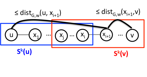
(a) Case 1: $j\leq i+1$

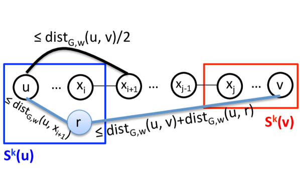
(b) Case 2: $j>i+1$.

Figure 1: Outline of the proof of Lemma 5.3

We now consider two cases (see Figure 1 for an outline). First, if $j\leq i+1$, then we have $x_{i+1}\in S^{k}(u)\cap S^{k}(v)$. This means that $w_{u}(x_{i+1},v)=w^{\prime}(x_{i+1},v)=\operatorname{\sf dist}_{G,w}(x_{i+1},v)$.

$$\operatorname{\sf dist}_{G_{u},w_{u}}(u,v) \leq w_{u}(u,x_{i+1})+w_{u}(x_{i+1},v)$$

$$=w^{\prime}(u,x_{i+1})+w^{\prime}(x_{i+1},v)$$

$$=\operatorname{\sf dist}_{G,w}(u,x_{i+1})+\operatorname{\sf dist}_{G,w}(x_{i+1},v)$$

$$=\operatorname{\sf dist}_{G,w}(u,v).$$

Now we consider the second case where $j>i+1$. In this case, we have that either

$$\operatorname{\sf dist}_{G,w}(u,x_{i+1})\leq\operatorname{\sf dist}_{G,w}(u,v)/2~{}~{}~{}\mbox{or}~{}~{}~{}\operatorname{\sf dist}_{G,w}(v,x_{j-1})\leq\operatorname{\sf dist}_{G,w}(u,v)/2\,.$$

Since the analyses for both cases are essentially the same, we will only show the analysis when $\operatorname{\sf dist}_{G,w}(u,x_{i+1})\leq\operatorname{\sf dist}_{G,w}(u,v)/2$. Observe that, with high probability, there is a random node $r\in R$ that is in $S^{k}(u)$ since $|S^{k}(u)|\geq\sqrt{n}$ and $R$ consists of $\tilde{\Theta}(\sqrt{n})$ random nodes (see Fact 4.4). Recall that, for every node $z$,

$$w_{u}(r,z)\leq d^{\prime\prime}(r,z)\leq(1+o(1))\operatorname{\sf dist}_{G,w}(r,z).$$

It follows that

$$\operatorname{\sf dist}_{G_{u},w_{u}}(u,v) \leq w_{u}(u,r)+w_{u}(r,v)$$ (10)

$$\leq(1+o(1))(\operatorname{\sf dist}_{G,w}(u,r)+\operatorname{\sf dist}_{G,w}(r,v))$$ (11)

$$\leq(1+o(1))(\operatorname{\sf dist}_{G,w}(u,r)+(\operatorname{\sf dist}_{G,w}(u,r)+\operatorname{\sf dist}_{G,w}(u,v)))$$ (12)

$$\leq(1+o(1))(2\operatorname{\sf dist}_{G,w}(u,x_{i+1})+\operatorname{\sf dist}_{G,w}(u,v))$$ (13)

$$\leq(2+o(1))\operatorname{\sf dist}_{G,w}(u,v).$$ (14)

Equation 12 is by triangle inequality. Equation 13 is because $r\in S_{u}$ and $x_{i+1}\notin S_{u}$. Equation 14 is because of the assumption that $\operatorname{\sf dist}_{G,w}(u,x_{i+1})\leq\operatorname{\sf dist}_{G,w}(u,v)/2$. ∎

6 Lower Bound for Approximating APSP (Proof of Observation 1.4)

See 1.4

Proof.

Our proof simply formalizes the fact that a node needs to receive at least $n$ bits of information in order to know its distance to all other nodes. We start from the following messag sending problem: Alice receive a $\beta$-bit binary vector, denoted by $\langle x_{1},\ldots,x_{\beta}\rangle$, where we set $\beta=n-2$. She wants to send this vector to Bob. Intuitively, to be sure that Bob gets the value of the vector correctly with a good probability, i.e. with probability at least $1-\epsilon$ for some small $\epsilon>0$, Alice has to send $\Omega(\beta)$ bits to Bob, regardless of what Bob sends to her. This fact can be formally proved in many ways (e.g., by using communication complexity lower bounds) and is true even in the quantum setting (see, e.g., Holevo’s theorem [Hol73]).

Now, let $\mathcal{A}$ be an $\alpha(n)$-approximation $T$-time algorithm for weighted APSP. We show that Alice can use $\mathcal{A}$ to send her message to Bob using $O(T\log n)$ bits, as follows. Construct a graph $G$ consisting of $n=\beta+2$ nodes, denoted by $a_{1},\ldots,a_{\beta}$, $a^{*}$ and $b$. There are edges between all nodes to $a^{*}$. The weight of edge $a^{*}b$ is always $w(a^{*}b)=1$. Weight of every edge $a_{i}a^{*}$ is set by Alice: if $x_{i}=1$ then she sets weight of $a_{i}a^{*}$ to $w(a_{i}a^{*})=1$; otherwise she sets it to $w(a_{i}a^{*})=2\alpha(n)$. Then, Alice simulates $\mathcal{A}$ on $a_{1},\ldots,a_{\beta}$ and $a^{*}$, and Bob simulates $\mathcal{A}$ on $b$. If $\mathcal{A}$ wants to send any message from $a^{*}$ to $b$, Alice will send this message to Bob so that Bob can continue simulating $b$. Similarly, if $\mathcal{A}$ wants to send any message from $b$ to $a^{*}$, Bob will send this message to Alice so that Alice can continue simulating $a^{*}$. If $\mathcal{A}$ finishes in $T$ rounds, then Alice will send at most $O(T\log n)$ bits to Bob in total.

Observe that, for any $i$, if $x_{i}=1$ then $\operatorname{\sf dist}_{G,w}(a_{i},b)=2$; otherwise, $\operatorname{\sf dist}_{G,w}(a_{i},b)=2\alpha(n)+1$. Since $\mathcal{A}$ is $\alpha(n)$ approximation, $\mathcal{A}$ must answer $\tilde{\operatorname{\sf dist}}_{G,w}(a_{i},b)\leq 2\alpha(n)$ if $x_{i}=1$; otherwise, $\mathcal{A}$ must answer $\tilde{\operatorname{\sf dist}}_{G,w}(a_{i},b)\geq 2\alpha(n)+1$. Since $\tilde{\operatorname{\sf dist}}_{G,w}(a_{i},b)$ is known to $b$, Bob can get the value of $\tilde{\operatorname{\sf dist}}_{G,w}(a_{i},b)$ by reading it from $b$ (which he is simulating). Then he can reconstructs $x_{i}$. Thus, Bob can reconstruct all bits $x_{1},\ldots,x_{\beta}$ after getting $O(T\log n)$ bits from Alice. The lower bound of the message sending problem thus implies that $T=\Omega(\beta/\log n)=\Omega(n/\log n)$.

Note that since the highest weight we can put on an edge is $\operatorname{poly}(n)$, we require that $\alpha(n)\leq\operatorname{poly}(n)$. We use the same argument for the unweighted case, but this time we use $\beta=n/\alpha(n)$ and replace an edge of weight $2\alpha(n)$ by a path of length $2\alpha(n)$. ∎

Note that in the proof above we show a lower bound for computing distances between all pairs of nodes. Since the lower bound graph is a star, the routing problem is trivial (since there is always one option to send a message). We can easily modify the above graph to give the same lower bound for the routing problem on weighted graphs: First, instead of using weight $2\alpha(n)$ in the graph above, use weight $2\alpha^{2}(n)+\alpha(n)$ instead. Second, add a new node $c$ and edges of weight $2\alpha(n)$ between $c$ and all nodes $a_{1}$ and an edge of weight $1$ between $c$ and $b$. Observe that if $x_{i}=1$, then we have to route a message through $a^{*}$, giving a distance of $2$ (while routing through $c$ gives a distance of $2\alpha(n)+1$. If $x_{i}=0$, we should route through $c$ which gives a distance of $2\alpha(n)+1$ since routing through $a^{*}$ will cost $2\alpha^{2}(n)+\alpha(n)+1$.

7 Open Problems

The main question left by our SSSP algorithm is the following.

Problem 7.1.

Close the gap between the upper bound of $\tilde{O}(n^{1/2}{\sf D}^{1/4})$ presented in this paper and the lower bound of $\tilde{\Omega}(n^{1/2})$ presented in [DHK⁺12] for $(1+\epsilon)$-approximating the single-source shortest paths problem on general networks.

Improving the current upper bound is important since there are many problems that can be potentially solved by using the same technique. Moreover, giving a lower bound in the form $\tilde{\Omega}(n^{1/2}{\sf D}^{\delta})$ for some $\delta>0$ will be quite surprising since such lower bound has not been observed before. It should also be fairly interesting to refine our upper bound to achieve a $\tilde{O}(n^{1/2}{\sf D}^{\epsilon})$-time $O(1/\epsilon)$-approximation algorithm for any $\delta>0$. Another question that should be very interesting is understanding the exact case:

Problem 7.2.

Can we solve SSSPexactly in sublinear-time?

It is also interesting to solve APSPexactly in linear-time (recall that sublinear-time is not possible). In some settings, an exact algorithm for computing shortest paths is crucial; e.g. some Internet protocols such as OSPF and IS-IS use edge weights to control the traffic and using an approximate shortest paths with this protocol is unacceptable. The next question is a generalization of our SSSP:

Problem 7.3 (Asymmetric SSSP).

How fast can we solve SSSP on networks whose edge weights could be asymmetric, i.e. if we think of each edge $uv$ as two directed edges $\overrightarrow{uv}$ and $\overrightarrow{vu}$, it is possible that $w(\overrightarrow{uv})\neq w(\overrightarrow{vu})$.

Note that we are particularly interested in the case where weights do not affect communication; in other words, if $u$ can send a message to $v$, then $v$ can also send a message to $u$. Also note that our light-weight SSSP algorithm can be used to solve this problem (but not the shortest-path diameter reduction technique). By adjusting parameters appropriately, we can $(1+\epsilon)$-approximate this problem in $\tilde{O}(\min(n^{2/3},n^{1/2}D^{1/2}))$ time. In fact, improving this running time for the following very special case seems challenging already:

Problem 7.4 ($s$-$t$ Reachability Problem).

Given a directed graph $G$ and two special nodes $s$ and $t$, we want to know whether there is a directed path from $s$ to $t$. The communication network is the underlying undirected graph; i.e. the communication can be done independent of edge directions and the diameter ${\sf D}$ is defined to be the diameter of the underlying undirected graph. Can we answer this question in $\tilde{O}(\sqrt{n}+{\sf D})$ time?

This problem shows limitations of the techniques presented in this paper, and we believe that solving it will give a new insight into solving all above open problems. Our last set of questions:

Problem 7.5.

Can we improve the $\tilde{O}(n^{1/2})$-time upper bound for SSSP on fully-connected networks while keeping the approximation ratio small (say, at most two)? Is it possible to prove a nontrivial $\omega(1)$ lower bound?

Note that the last question was asked earlier by Elkin [Elk04].

8 Acknowledgement

The sublinear-time SSSP algorithm was inspired by the discussions with Jittat Fakcharoenphol and Jakarin Chawachat, who refused to co-author this paper. Several techniques borrowed from dynamic graph algorithms benefit from many intensive discussions with Sebastian Krinninger and Monika Henzinger. I also would like to thank Radhika Arava and Peter Robinson for explaining the algorithm of Baswana and Sen [BS07] to him and Gopal Pandurangan, Chunming Li, Anisur Rahaman, David Peleg, Atish Das Sarma, Parinya Chalermsook, Bundit Laekhanukit, Boaz Patt-Shamir, Shay Kutten, Christoph Lenzen, Stephan Holzer, Mohsen Ghaffari, Nancy Lynch, and Mikkel Thorup, for discussions, comments, and pointers to related results. I also thank all reviewers of STOC 2014 for many thoughtful comments.

References

- [AHT92] John K. Antonio, Garng M. Huang, and Wei Kang Tsai. A fast distributed shortest path algorithm for a class of hierarchically clustered data networks. IEEE Trans. Computers, 41(6):710–724, 1992.
- [APRU12] John Augustine, Gopal Pandurangan, Peter Robinson, and Eli Upfal. Towards robust and efficient computation in dynamic peer-to-peer networks. In SODA, pages 551–569, 2012.
- [AR82] J. Abram and I. Rhodes. Some shortest path algorithms with decentralized information and communication requirements. Automatic Control, IEEE Transactions on, 27(3):570–582, 1982.
- [AR93] Yehuda Afek and Moty Ricklin. Sparser: A paradigm for running distributed algorithms. J. Algorithms, 14(2):316–328, 1993.
- [Bel58] R. Bellman. On a routing problem. Quarterly of Applied Mathematics, 16:87–90, 1958.
- [Ber13] Aaron Bernstein. Maintaining shortest paths under deletions in weighted directed graphs: [extended abstract]. In STOC, pages 725–734, 2013.
- [BHP12] Andrew Berns, James Hegeman, and Sriram V. Pemmaraju. Super-fast distributed algorithms for metric facility location. In ICALP (2), pages 428–439, 2012.
- [BS07] Surender Baswana and Sandeep Sen. A simple and linear time randomized algorithm for computing sparse spanners in weighted graphs. Random Struct. Algorithms, 30(4):532–563, 2007. Also in ICALP’03.
- [Coh00] Edith Cohen. Polylog-time and near-linear work approximation scheme for undirected shortest paths. J. ACM, 47(1):132–166, 2000. Announced at STOC 1994.
- [DDP12] Atish Das Sarma, Michael Dinitz, and Gopal Pandurangan. Efficient computation of distance sketches in distributed networks. In SPAA, pages 318–326, 2012.
- [DFI05] Camil Demetrescu, Irene Finocchi, and Giuseppe F. Italiano. Handbook on Data Structures and Applications, chapter 36: Dynamic Graphs. Dinesh Mehta and Sartaj Sahni (eds.), CRC Press Series, in Computer and Information Science, 2005.
- [DHK+12] Atish Das Sarma, Stephan Holzer, Liah Kor, Amos Korman, Danupon Nanongkai, Gopal Pandurangan, David Peleg, and Roger Wattenhofer. Distributed verification and hardness of distributed approximation. SIAM J. Comput., 41(5):1235–1265, 2012. Announced at STOC 2011.
- [DLP12] Danny Dolev, Christoph Lenzen, and Shir Peled. ”tri, tri again”: Finding triangles and small subgraphs in a distributed setting - (extended abstract). In DISC, pages 195–209, 2012.
- [DNPT13] Atish Das Sarma, Danupon Nanongkai, Gopal Pandurangan, and Prasad Tetali. Distributed random walks. J. ACM, 60(1):2, 2013. Also in PODC’09 and PODC’10.
- [EFK+12] Yuval Emek, Pierre Fraigniaud, Amos Korman, Shay Kutten, and David Peleg. Notions of connectivity in overlay networks. In SIROCCO, pages 25–35, 2012.
- [EKNP12] Michael Elkin, Hartmut Klauck, Danupon Nanongkai, and Gopal Pandurangan. Quantum distributed network computing: Lower bounds and techniques. CoRR, abs/1207.5211, 2012.
- [Elk04] Michael Elkin. Distributed approximation: a survey. SIGACT News, 35(4):40–57, 2004.
- [Elk05] Michael Elkin. Computing almost shortest paths. ACM Transactions on Algorithms, 1(2):283–323, 2005. Also in PODC’01.
- [Elk06] Michael Elkin. An unconditional lower bound on the time-approximation trade-off for the distributed minimum spanning tree problem. SIAM J. Comput., 36(2):433–456, 2006. Also in STOC’04.
- [EZ06] Michael Elkin and Jian Zhang. Efficient algorithms for constructing (1+epsilon, beta)-spanners in the distributed and streaming models. Distributed Computing, 18(5):375–385, 2006. Also in PODC’04.
- [FHW12] Silvio Frischknecht, Stephan Holzer, and Roger Wattenhofer. Networks cannot compute their diameter in sublinear time. In SODA, pages 1150–1162, 2012.
- [For56] Lester R. Ford. Network Flow Theory. Report P-923, The Rand Corporation, 1956.
- [FRT04] Jittat Fakcharoenphol, Satish Rao, and Kunal Talwar. A tight bound on approximating arbitrary metrics by tree metrics. J. Comput. Syst. Sci., 69(3):485–497, 2004. Also in STOC’03.
- [GK81] D.H. Greene and D.E. Knuth. Mathematics for the analysis of algorithms. Progress in computer science. Birkhäuser, 1981.
- [GK13] Mohsen Ghaffari and Fabian Kuhn. Distributed minimum cut approximation. In DISC, pages 1–15, 2013.
- [GKP98] Juan A. Garay, Shay Kutten, and David Peleg. A sublinear time distributed algorithm for minimum-weight spanning trees. SIAM J. Comput., 27(1):302–316, 1998. Also in FOCS’93.
- [Hal97] S. Haldar. An ‘all pairs shortest paths’ distributed algorithm using 2n2 messages. J. Algorithms, 24(1):20–36, 1997.
- [Hol73] A. S. Holevo. Bounds for the quantity of information transmitted by a quantum communication channel. Problemy Peredachi Informatsii, 9(3):3–11, 1973. English translation in Problems of Information Transmission, 9:177–183, 1973.
- [Hol13] Stephan Holzer. Distance Computation, Information Dissemination, and Wireless Capacity in Networks, Diss. ETH No. 21444. Phd thesis, ETH Zurich, Zurich, Switzerland, 2013.
- [HW12] Stephan Holzer and Roger Wattenhofer. Optimal distributed all pairs shortest paths and applications. In PODC, pages 355–364, 2012.
- [KKM+12] Maleq Khan, Fabian Kuhn, Dahlia Malkhi, Gopal Pandurangan, and Kunal Talwar. Efficient distributed approximation algorithms via probabilistic tree embeddings. Distributed Computing, 25(3):189–205, 2012. Announced at PODC 2008.
- [KKP13] Liah Kor, Amos Korman, and David Peleg. Tight bounds for distributed minimum-weight spanning tree verification. Theory Comput. Syst., 53(2):318–340, 2013.
- [KP98] Shay Kutten and David Peleg. Fast distributed construction of small k-dominating sets and applications. J. Algorithms, 28(1):40–66, 1998.
- [KP08] Maleq Khan and Gopal Pandurangan. A fast distributed approximation algorithm for minimum spanning trees. Distributed Computing, 20(6):391–402, 2008. Also in DISC’06.
- [KS92] Philip N. Klein and Sairam Sairam. A parallel randomized approximation scheme for shortest paths. In STOC, pages 750–758, 1992.
- [Len13] Christoph Lenzen. Optimal deterministic routing and sorting on the congested clique. In PODC, pages 42–50, 2013.
- [LMR94] Frank Thomson Leighton, Bruce M. Maggs, and Satish Rao. Packet Routing and Job-Shop Scheduling in O(Congestion + Dilation) Steps. Combinatorica, 14(2):167–186, 1994. Also in FOCS’88.
- [LPS13] Christoph Lenzen and Boaz Patt-Shamir. Fast routing table construction using small messages: extended abstract. In STOC, pages 381–390, 2013.
- [LPSP06] Zvi Lotker, Boaz Patt-Shamir, and David Peleg. Distributed mst for constant diameter graphs. Distributed Computing, 18(6):453–460, 2006.
- [LPSPP05] Zvi Lotker, Boaz Patt-Shamir, Elan Pavlov, and David Peleg. Minimum-Weight Spanning Tree Construction in O(log log n) Communication Rounds. SIAM J. Comput., 35(1):120–131, July 2005. Also in SPAA’03.
- [LPSR09] Zvi Lotker, Boaz Patt-Shamir, and Adi Rosén. Distributed approximate matching. SIAM J. Comput., 39(2):445–460, 2009.
- [LW11] Christoph Lenzen and Roger Wattenhofer. Tight bounds for parallel randomized load balancing: extended abstract. In Proceedings of the 43rd annual ACM symposium on Theory of computing, STOC ’11, pages 11–20, New York, NY, USA, 2011. ACM.
- [Lyn96] Nancy A. Lynch. Distributed Algorithms. Morgan Kaufmann Publishers Inc., San Francisco, CA, USA, 1996.
- [MU05] Michael Mitzenmacher and Eli Upfal. Probability and computing - randomized algorithms and probabilistic analysis. Cambridge University Press, 2005.
- [Nan14] Danupon Nanongkai. Brief announcement: Almost-tight approximation distributed algorithm for minimum cut. In PODC, 2014.
- [Pel00] D. Peleg. Distributed computing: a locality-sensitive approach. Society for Industrial and Applied Mathematics, Philadelphia, PA, USA, 2000.
- [Pet10] Seth Pettie. Distributed algorithms for ultrasparse spanners and linear size skeletons. Distributed Computing, 22(3):147–166, 2010. Also in PODC’08.
- [PR00] David Peleg and Vitaly Rubinovich. A near-tight lower bound on the time complexity of distributed minimum-weight spanning tree construction. SIAM J. Comput., 30(5):1427–1442, 2000. Also in FOCS’99.
- [PRT12] David Peleg, Liam Roditty, and Elad Tal. Distributed algorithms for network diameter and girth. In ICALP (2), pages 660–672, 2012.
- [PST11] Boaz Patt-Shamir and Marat Teplitsky. The round complexity of distributed sorting: extended abstract. In Proceedings of the 30th annual ACM SIGACT-SIGOPS symposium on Principles of distributed computing, PODC ’11, pages 249–256, New York, NY, USA, 2011. ACM.
- [PT11] David Pritchard and Ramakrishna Thurimella. Fast computation of small cuts via cycle space sampling. ACM Transactions on Algorithms, 7(4):46, 2011. Also in ICALP’08.
- [RT85] Prabhakar Raghavan and Clark D. Thompson. Provably good routing in graphs: Regular arrays. In STOC, pages 79–87, 1985.
- [San06] Nicola Santoro. Design and Analysis of Distributed Algorithms (Wiley Series on Parallel and Distributed Computing). Wiley-Interscience, 2006.
- [Som12] Christian Sommer. Shortest-path queries in static networks, 2012. submitted.
- [Su14] Hsin-Hao Su. Brief announcement: A distributed minimum cut approximation scheme. In SPAA, 2014.
- [Thu97] Ramakrishna Thurimella. Sub-linear distributed algorithms for sparse certificates and biconnected components. J. Algorithms, 23(1):160–179, 1997. Also in PODC’95.
- [TZ05] Mikkel Thorup and Uri Zwick. Approximate distance oracles. J. ACM, 52(1):1–24, 2005. Also in STOC’11.
- [UY91] Jeffrey D. Ullman and Mihalis Yannakakis. High-probability parallel transitive-closure algorithms. SIAM J. Comput., 20(1):100–125, 1991.