Synergy and redundancy in the Granger causal analysis of dynamical networks

Abstract

We analyze by means of Granger causality the effect of synergy and redundancy in the inference (from time series data) of the information flow between subsystems of a complex network. Whilst we show that fully conditioned Granger causality is not affected by synergy, the pairwise analysis fails to put in evidence synergetic effects. In cases when the number of samples is low, thus making the fully conditioned approach unfeasible, we show that partially conditioned Granger causality is an effective approach if the set of conditioning variables is properly chosen. We consider here two different strategies (based either on informational content for the candidate driver or on selecting the variables with highest pairwise influences) for partially conditioned Granger causality and show that depending on the data structure either one or the other might be valid. On the other hand, we observe that fully conditioned approaches do not work well in presence of redundancy, thus suggesting the strategy of separating the pairwise links in two subsets: those corresponding to indirect connections of the fully conditioned Granger causality (which should thus be excluded) and links that can be ascribed to redundancy effects and, together with the results from the fully connected approach, provide a better description of the causality pattern in presence of redundancy. We finally apply these methods to two different real datasets. First, analyzing electrophysiological data from an epileptic brain, we show that synergetic effects are dominant just before seizure occurrences. Second, our analysis applied to gene expression time series from HeLa culture shows that the underlying regulatory networks are characterized by both redundancy and synergy.

I Introduction

Living organisms can be modeled as an ensemble of complex physiological systems, each with its own regulatory mechanism and all continuously interacting between them ivanov . Therefore inferring the interactions within and between these modules is a crucial issue. Over the last years the interaction structure of many complex systems has been mapped in terms of networks, which have been successfully studied using tools from statistical physics barabasi . Dynamical networks have modeled physiological behavior in many applications; examples range from networks of neurons netnn , genetic networks gennet , protein interaction nets protein and metabolic networks metabolic ; metabolic1 ; cortes2011 .

The inference of dynamical networks from time series data is related to the estimation of the information flow between variables pereda2005 ; see also book1 ; book2 . Granger causality (GC) granger ; sethbressler has emerged as a major tool to address this issue. This approach is based on prediction: if the prediction error of the first time series is reduced by including measurements from the second one in the linear regression model, then the second time series is said to have a Granger causal influence on the first one. It has been shown that GC is equivalent to transfer entropy schreiber in the Gaussian approximation barnett and for other distributions hac . See vicente for a discussion about applicability of this notion in neuroscience, and njp for a discussion on the reliability of GC for continuous dynamical processes. It is worth stressing that several forms of coupling may mediate information flow in the brain, see bart1 ; bart2 . The combination of GC and complex networks theory is also a promising line of research njp1 .

The pairwise Granger analysis (PWGC) consists in assessing GC between each pair of variables, independently of the rest of the system. It is well known that the pairwise analysis cannot disambiguate direct and indirect interactions among variables. The most straightforward extension, the conditioning approach geweke , removes indirect influences by evaluating to which extent the predictive power of the driver on the target decreases when the conditioning variable is removed. It has to be noted however that, even though its limitations are well known, the pairwise GC approach is still used in situations where the number of samples is limited and a fully conditioned approach is unfeasible. As a convenient alternative to this suboptimal solution, a partially conditioned approach, consisting in conditioning on a small number of variables, chosen as the most informative ones for the driver node, has been proposed partialold ; this approach leads to results very close to those obtained with a fully conditioned analysis and even more accurate in the presence of a small number of samples partialBC . We remark that the use of partially conditioned Granger causality (PCGC) may be useful also in non-stationary conditions, where the GC pattern has to be estimated on short time windows.

Sometimes though a fully conditioned (CGC) approach can encounter conceptual limitations, on top of the practical and computational ones: in the presence of redundant variables the application of the standard analysis leads to underestimation of influences noipre . Redundancy and synergy are intuitive yet elusive concepts, which have been investigated in different fields, from pure information theory griffith ; harder ; Lizier , to machine learning yang and neural systems schnei ; gat , with definitions that range from the purely operative to the most conceptual ones. When analyzing interactions in multivariate time series, redundancy may arise if some channels are all influenced by another signal that is not included in the regression; another source of redundancy may be the emergence of synchronization in a subgroup of variables, without the need of an external influence. Redundancy manifests itself through a high degree of correlation in a group of variables, both for instantaneous and lagged influences. Several approaches have been proposed in order to reduce dimensionality in multivariate sets eliminating redundancy, relying on generalized variance barnettpre , principal components analysis zhou , or Granger causality itself noipla .

A complementary concept to redundancy is synergy. The synergetic effects that we address here, related to the analysis of dynamical influences in multivariate time series, are similar to those encountered in sociological and psychological modeling, where suppressors is the name given to variables that increase the predictive validity of another variable after its inclusion into a linear regression equation conger ; see thompson for examples of easily explainable suppressor variables in multiple regression research. Redundancy and synergy have been further connected to information transfer in preExpansion ,where an expansion of the information flow has been proposed to put in evidence redundant and synergetic multiplets of variables. Other information-based approaches have also addressed the issue of collective influence Chicharro ; Lizier . The purpose of this paper is to provide evidence that in addition to the problem related to indirect influence, PWGC shows another relevant pitfall: it fails to detect synergetic effects in the information flow, in other words it does not account for the presence of subsets of variables that provide some information about the future of a given target only when all the variables are used in the regression model. We remark that since it processes the system as a whole, CGC evidences synergetic effects; when the number of samples is low, PCGC can detect synergetic effects too, after an adequate selection of the conditioning variables.

The paper is organized as follows. In the next section we briefly recall the concepts of GC and PCGC. In section III we describe some toy systems illustrating how redundancy can affect the results of CGC, whilst indirect interactions and synergy are the main problems inherent to PWGC. In section IV we provide evidence of synergetic effects in epilepsy: we analyze electroencephalographic recordings from an epileptic patient corresponding to ten seconds before the seizure onset; we show that the two contacts which constitute the putative seizure onset act as synergetic variables driving the rest of the system. The pattern of information transfer evidences the actual seizure onset only when synergy is correctly considered.

In section V we propose an approach that combines PWGC and CGC to evidence the pairwise influences due only to redundancy and not recognized by CGC. The conditioned GC pattern is used to partition the pairwise links in two sets: those which are indirect influences between the measured variables, according to CGC, and those which are not explained as indirect relationships. The unexplained pairwise links, presumably due to redundancy, are thus retained to complement the information transfer pattern discovered by CGC. In cases where the number of samples is so low that a fully multivariate approach is unfeasible, PCGC may be applied instead of CGC. We also address here the issue of variables selection for PCGC, and consider a novel strategy for the selection of variables: for each target variable, one selects the variables sending the highest amount of information to that node as indicated by a pairwise analysis. By construction, this new selection strategy works more efficiently when the interaction graph has a tree structure: indeed in this case conditioning on the parents of the target node ensures that indirect influences will be removed. In the epilepsy example the selection based on the mutual information with the candidate driver provides results closer to those obtained by CGC. We finally apply the proposed approach on time series of gene expressions, extracted from a data-set from the HeLa culture. Section VI summarizes our conclusions.

II Insights into Granger causality

Granger causality is a powerful and widespread data-driven approach to determine whether and how two time series exert direct dynamical influences on each other hla . A convenient nonlinear generalization of GC has been implemented in noipre2 , exploiting the kernel trick, which makes computation of dot products in high-dimensional feature spaces possible using simple functions (kernels) defined on pairs of input patterns. This trick allows the formulation of nonlinear variants of any algorithm that can be cast in terms of dot products, for example Support Vector Machines vapnik . Hence in noipre2 the idea is still to perform linear Granger causality, but in a space defined by the nonlinear features of the data. This projection is conveniently and implicitly performed through kernel functions shawe and a statistical procedure is used to avoid over-fitting.

Quantitatively, let us consider $n$ time series $\{x_{\alpha}(t)\}_{\alpha=1,\ldots,n}$; the lagged state vectors are denoted

$$X_{\alpha}(t)=\left(x_{\alpha}(t-m),\ldots,x_{\alpha}(t-1)\right),$$

$m$ being the order of the model (window length). Let $\epsilon\left(x_{\alpha}|{\bf X}\right)$ be the mean squared error prediction of $x_{\alpha}$ on the basis of all the vectors ${\bf X}=\{X_{\beta}\}_{\beta=1}^{n}$ (corresponding to the kernel approach described in noiprl ). The multivariate Granger causality index $\delta_{mv}(\beta\to\alpha)$ is defined as follows: consider the prediction of $x_{\alpha}$ on the basis of all the variables but $X_{\beta}$ and the prediction of $x_{\alpha}$ using all the variables, then the GC is the (normalized) variation of the error in the two conditions, i.e.

$$\delta_{mv}(\beta\to\alpha)=\log{\epsilon\left(x_{\alpha}|{\bf X}\setminus X_{\beta}\right)\over\epsilon\left(x_{\alpha}|{\bf X}\right)};$$ (1)

In ancona it has been shown that not all the kernels are suitable to estimate GC. Two important classes of kernels which can be used to construct nonlinear GC measures are the inhomogeneous polynomial kernel (whose features are all the monomials in the input variables up to the $p$-th degree; $p=1$ corresponds to linear Granger causality) and the Gaussian kernel.

The pairwise Granger causality is given by:

$$\delta_{bv}(\beta\to\alpha)=\log{\epsilon\left(x_{\alpha}|X_{\alpha}\right)\over\epsilon\left(x_{\alpha}|X_{\alpha},X_{\beta}\right)}.$$ (2)

The partially conditioned Granger causality is defined as follows. Let $\bf{Y}$ be the variables in $\bf{X}$, excluding $X_{\alpha}$ and $X_{\beta}$, then (1) can be written as:

$$\delta_{c}^{\bf{Y}}(\beta\to\alpha)=\log{\epsilon\left(x_{\alpha}|X_{\alpha},\bf{Y}\right)\over\epsilon\left(x_{\alpha}|X_{\alpha},X_{\beta},\bf{Y}\right)}.$$ (3)

When $\bf{Y}$ is only a subset of the total number of variables in $\bf{X}$ not containing $X_{\alpha}$ and $X_{\beta}$, then $\delta_{c}^{\bf{Y}}$ is called the partially conditioned Granger causality (PCGC). In partialold the set $\bf{Y}$ is chosen as the most informative for $X_{\beta}$. Here we will also consider an alternative strategy: fixing a small number $k$, we select ${\bf Y}=\{X_{\gamma}\}_{\gamma=1}^{k}$ as the $k$ variables with the maximal pairwise GC $\delta_{bv}(\gamma\to\alpha)$ w.r.t. that target node, excluding $X_{\beta}$.

III Examples

In this section we provide some typical examples to remark possible problems that pairwise and fully conditioned analysis may encounter.

III.1 Indirect GC among measured variables

We consider the following lattice of ten unidirectionally coupled noisy logistic maps, with

$$x_{1}(t)=f\left(x_{1}(t-1)\right)+0.01\eta_{1}(t),$$ (4)

and

$$x_{i}(t)=(1-\rho)f\left(x_{i}(t-1)\right)+\rho f\left(x_{i-1}(t-1)\right)+0.01\eta_{i}(t),$$ (5)

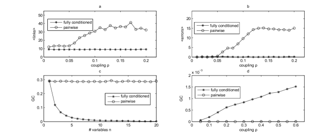
Figure 1: (a) The average number of links as a function of the coupling $\rho$, over 100 runs of 2000 time points, retrieved by PWGC and CGC on the coupled map lattice described in the text, eqs. (4-5). (b) On the coupled map lattice, the average error (sum of type I errors and type II errors in the recovery of causal interactions) by PCGC, obtained by the IB strategy and by PB, is plotted versus the coupling $\rho$. Errors are averaged over 100 runs of 2000 time points. (c) For the example dealing with redundancy, CGC and PWGC are plotted versus the number of variables. Results are averaged over 100 runs of 1000 time points (d) For the example dealing with synergy, CGC and PWGC are plotted versus the coupling $\rho$. Results are averaged over 100 runs of 1000 time points

with $i=2,\ldots,10$. Variables $\eta$ are unit variance Gaussian noise terms. The transfer function is given by $f(x)=1-1.8x^{2}$. In this system the first map is evolving autonomously, whilst the other maps are influenced by the previous ones with coupling $\rho$, thus forming a cascade of interactions. In figure 1a we plot as a function of $\rho$ the number of GC interactions found by PWGC and CGC, using the method described in noipre with the inhomogeneous polynomial kernel of degree two. The CGC output is the correct one (nine links) whilst the PWGC output also accounts for indirect influences and therefore fails to provide the underlying network of interactions. On this example we have also tested PCGC, see figure 1b. We considered just one conditioning variable, chosen according to the two strategies described above. Firstly we consider the most informative w.r.t. the candidate driver, as described in partialold ; we call this strategy information based (IB). Secondly, we choose the variable characterized by the maximal pairwise influence to the target node, a pairwise based (PB) rule. The PB strategy yields the correct result in this example, whilst the IB one fails when only one conditioning variable is used and requires more than one conditioning variables to provide the correct output. This occurrence is due to the tree topology of the interactions in this example, which favors PB selecting by construction the parents of each node.

III.2 Redundancy due to a hidden source

We show here how redundancy constitutes a problem for CGC. Let $h(t)$ be a zero mean and unit variance hidden Gaussian variable, influencing $n$ variables $x_{i}(t)=h(t-1)+s\eta_{i}(t)$, and let $w(t)=h(t-2)+s\eta_{0}(t)$ be another variable who is influenced by $h$ but with a larger delay. The $\{\eta\}$ variables are unit variance Gaussian noise and s controls the noise level. In figure 1c we depict both the linear PWGC and the linear CGC from one of the x’s to w (note that h is not used in the regression model). As $n$ increases, the conditioned GC vanishes as a consequence of redundancy. The GC relation which is found in the pairwise analysis is not revealed by CGC because $\{x\}$ variables are maximally correlated and thus $x_{i}$ drives $w$ only in the absence of any other variables.

The correct way to describe the information flow pattern in this example, where the true underlying source $h$ is unknown, is that all the $\{x\}$ variables are sending the same information to w, i.e. that variables $\{x\}$ constitute a redundant multiplet w.r.t. the causal influence to w. This pattern follows from observing that for all x’s CGC vanishes whilst PWGC does not vanish. This example shows that, in presence of redundancy, the CGC pattern alone is not sufficient to describe the information flow pattern of the system, and also PWGC should be taken into account.

III.3 Synergetic contributions

Let us consider three unit variance iid Gaussian noise terms $x_{1}$, $x_{2}$ and $x_{3}$. Let

$$x_{4}(t)=0.1(x_{1}(t-1)+x_{2}(t-1))+\rho x_{2}(t-1)x_{3}(t-1)+0.1\eta(t).$$

Considering the influence $3\to 4$, the CGC reveals that $3$ is influencing $4$, whilst PWGC fails to detect this causal relationship, see figure 1d, where we use the method described in noipre with the inhomogeneous polynomial kernel of degree two; $x_{2}$ is a suppressor variable for $x_{3}$ w.r.t. the influence on $x_{4}$. This example shows that PWGC fails to detect synergetic contributions. We remark that use of nonlinear GC is mandatory in this case to put in evidence the synergy between $x_{2}$ and $x_{3}$.

III.4 Redundancy due to synchronization

As another example, we consider a toy system made of five variables $\{x_{i}\}$. The first four constitute a multiplet made of a fully coupled lattice of noisy logistic maps with coupling $\rho$, evolving independently of the fifth. The fifth variable is influenced by the mean field from the coupled map lattice. The equations are, for $i=1,\ldots,4$,:

$$x_{i}(t)=(1-\rho)f\left(x_{i}(t-1)\right)+\rho\sum_{j=1,j\neq i}^{4}f\left(x_{j}(t-1)\right)+0.01\eta_{i}(t),$$ (6)

and

$$x_{5}(t)=\sum_{i=1}^{4}{x_{i}(t-1)\over 8}+\eta_{5}(t),$$ (7)

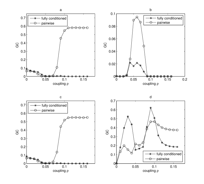
Figure 2: (a) The CGC and PWGC of the causal interaction $x_{1}\to x_{5}$ is plotted as a function of the coupling $\rho$ for the example dealing with redundancy due to synchronization, eqs. (6-7). The linear algorithms are used here and results are averaged over 100 runs of 2000 time points (b) The CGC and PWGC of the causal interaction between two variables in the multiplet is plotted as a function of the coupling $\rho$ for the example dealing with redundancy due to synchronization. The linear algorithms are used here and results are averaged over 100 runs of 2000 time points (c) The nonlinear CGC and PWGC of the causal interaction $x_{1}\to x_{5}$ is plotted as a function of the coupling $\rho$ for the example dealing with redundancy due to synchronization. The algorithm with the polynomial kernel of order 2 is used here and results are averaged over 100 runs of 2000 time points (d) The nonlinear CGC and PWGC of the causal interaction between two variables in the multiplet is plotted as a function of the coupling $\rho$ for the example dealing with redundancy due to synchronization. The algorithm with the polynomial kernel of order 2 is used here and results are averaged over 100 runs of 2000 time points.

where $\eta$ are unit variance Gaussian noise terms. Increasing the coupling $\rho$ among the variables in the multiplet $\{x_{1},x_{2},x_{3},x_{4}\}$, the degree of synchronization among these variables (measured e.g. by Pearson correlations) increases and they become almost synchronized for $\rho$ greater than 0.1 (complete synchronization cannot be achieved due to the noise terms); redundancy, in this example, arises due to complex inherent dynamics of the units. In figure 2 we depict both the causality from one variable in the multiplet ($x_{1}$; the same results hold fo r$x_{2}$, $x_{3}$ and $x_{4}$ ) to $x_{5}$, and the causality between pairs of variables in the multiplet: both linear and nonlinear PWGC and CGC are shown for the two quantities.

Concerning the causality $x_{1}\to x_{5}$, we note that, for low coupling, both PWGC and CGC, with linear or nonlinear kernel, correctly detect the causal interaction. Around the transition to synchronization, in a window centered at $\rho=0.05$, all the algorithms fail to detect the causality $x_{1}\to x_{5}$. In the almost synchronized regime, $\rho>0.1$, the fully conditioned approach continues to fail due to redundancy, whilst the PWGC provides correctly the causal influence, both using the linear and the nonlinear algorithm.

As far as the causal interactions within the multiplet are concerned, we note that using the linear approach we get small values of causality just at the transition, whilst we get zero values far from the transition. Using the nonlinear algorithm, which is the correct one in this example as the system is nonlinear, we obtain nonzero causality among the variables in the multiplet, using both PWGC or CGC: the resulting curves are non-monotonous as one may expect due to the inherent nonlinear dynamics. For $\rho>1$ nonzero GC is observed because of the noise which prevents the system to go in the complete synchronized state.

This example again shows that in presence of redundancy one should take into account both CGC and PWGC results. Moreover it also shows how nonlinearity may render extremely difficult the inference of interactions: in this system there is a range of values, corresponding to the onset of synchronization, in which all methods fail to provide the correct causal interaction.

IV Synergetic effects in the epileptic brain

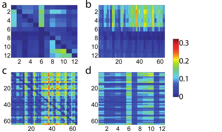
Figure 3: The PWGC is depicted for the epilepsy data. (a) PWGC between the contacts of the two DEs. (b) PWGC from DEs to CEs. (c) PWGC between CEs. (d) PWGC from CEs to DEs.

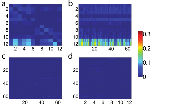
Figure 4: The CGC is depicted for the epilepsy data. (a) CGC between the contacts of the two DEs. (b) CGC from DEs to CEs. (c) CGC between CEs. (d) CGC from CEs to DEs.

As a real example we consider intracranial EEG recordings from a patient with drug-resistant epilepsy with an implanted array of $8\times 8$ cortical electrodes (CE) and two depth electrodes (DE) with six contacts each. The data are available at kol_web and further details on the dataset are given in kol_paper . Data were sampled at 400 Hz. We consider here a portion of data recorded in the preictal period, 10 seconds preceding the seizure onset. To handle this data, we use linear Granger causality with $m$ equal to five. In figure 3 we depict the PWGC between DEs (panel a), from DEs to CEs (panel b), between CEs (panel c) and from CEs to DEs (panel d). We note a complex pattern of bivariate interactions among CEs, whilst the first DE seems to be the subcortical drive to the cortex. We remark that there is no PWGC from the last two contacts of the second DE (channels 11 and 12) to CEs and neither to the contacts of the first DE. In figure 4 we depict the CGC among DEs (panel a), from DEs to CEs (panel b), among CEs (panel c) and from CEs to DEs (panel d). The scenario in the conditioned case is clear: the contacts 11 and 12, from the second DE, are the drivers both for the cortex and for the subcortical region associated to the first DE. These two contacts can be then associated to the seizure onset zone (SOZ). The high pairwise GC strength among CEs is due to redundancy, as these latter are all driven by the same subcortical source. Since the contact 12 is also driving the contact 11, see figure 4a, we conclude that the contact 12 is the closest to the SOZ, and that the contact 11 is a suppressor variable for it, because it is necessary to include it in the regression model to put in evidence the influence of 12 on the rest of the system. Conversely, the contact 12 acts as a suppressor for contact 11. We stress that the influence from contacts 11 and 12 to the rest of the system emerges only in the CGC and it is neglected by PWGC: these variables are synergetically influencing the dynamics of the system. To our knowledge this is the first time that synergetic effects are found in relation with epilepsy.

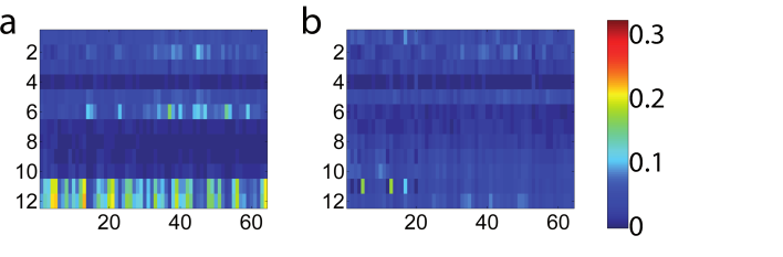
Figure 5: The PCGC is depicted for the epilepsy data. (a)PCGC from DEs to CEs, with IB strategy for variable selection. Note that the influences from DE11 are conditioned here on DE12, and the influences from DE11 are conditioned on DE 12, thus showing that these variables are suppressor among themselves. (b) PCGC from DEs to CEs, with PB strategy for variable selection.

On this data we also apply PCGC using one conditioning variable. The results are depicted in figure 5: using the IB strategy we obtain a pattern very close to the one from CGC, while this is not the case of PB. These results seem to suggest that IB works better in presence of redundancy, however we have not arguments to claim that this a general rule. It is worth mentioning that in presence of synergy the selection of variables for partial conditioning is equivalent to the search of suppressor variables.

V A combination of pairwise and conditioned Granger Causality

In the last sections we have shown that CGC encounters issues resulting in poor performance in presence of redundancy, and that information about redundancy may be obtained from the PWGC pattern. We develop here a strategy to combine the two approaches: some links inferred from PWGC are retained and added to those obtained from CGC. The PWGC links that are discarded are those which can be derived as indirect links from the CGC pattern. In the following we describe the proposed approach in detail.

Let $\Delta$ be the matrix of influences from CGC (or PCGC). Let $\Delta^{*}$ be the matrix from PWGC. Non-zero elements of $\Delta$ and $\Delta^{*}$ correspond to the estimated influences. Let these matrices be evaluated using a model of order $m$.

The matrix

$$M_{\alpha\beta}=\Delta^{\alpha}(\Delta^{\top})^{\beta}$$

contains paths of length $\alpha+\beta$ with delays in the range $[-\beta m+\alpha,\ldots,-\beta+\alpha m]$. Indeed:

$$M_{\alpha\beta}(i,j)=\sum_{i_{1}}\sum_{i_{2}}\cdots\sum_{i_{\alpha+\beta-1}}\Delta(i,i_{1})\Delta(i_{1},i_{2})\cdots\Delta(j,i_{\alpha+\beta-1});$$ (8)

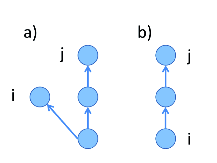
Figure 6: (a) The indirect influence $i\to j$ corresponding to a nonzero element of the matrix $\Delta^{2}\Delta^{\top}$. If $\Delta^{2}\Delta^{\top}(i,j)\neq 0$, then a common source influences $i$ and $j$ but with different lags. (b) The indirect causality $i\to j$ corresponding to nonzero elements of the matrix $\Delta^{2}$. If $\Delta^{2}(i,j)\neq 0$, then a third node acting as a mediator of the interaction $i\to j$.

since all elements of $\Delta$ are non-negative, it follows that $M_{\alpha\beta}(i,j)$ is not vanishing if and only if it is possible, in matrix $\Delta$, to go from node i to node j moving $\beta$ steps backward and $\alpha$ steps forward, where a step is allowed if the corresponding element of $\Delta$ is not zero. Therefore the nonzero elements of the matrix $M_{\alpha\beta}$ describe a situation where two nodes receive a common input from a third node which is $\alpha$ steps backward in time from one node, and $\beta$ steps backward in time in time from the other node. In other words, if the element $M_{\alpha\beta}(i,j)$ does not vanish, then there exist an indirect interaction between nodes $i$ and $j$ due to a common input. The circuit corresponding to $M_{21}$ is represented in figure 6a: if the element $M_{2,1}(i,j)$ is non-vanishing, then i and j are connected as in figure 6a .

Since the order of the model is $m$, a simple comparison between the delays from the common source to $i$ and $j$ demonstrates that the indirect influence corresponding to the non-zero element $M_{\alpha,\beta}(i,j)$ might be detected by PWGC only if

$$[-\beta m+\alpha,\ldots,-\beta+\alpha m]\cap[1,\ldots,m]\neq\emptyset;$$

this is equivalent to

$${\beta+1\over m}\leq\alpha\leq(\beta+1)m.$$

Now, the matrix $F_{\alpha}=\Delta^{\alpha},$ with $\alpha\geq 1$, contains paths of length $\alpha$ with delays in the range $[\alpha,\ldots,\alpha m]$, indeed:

$$F_{\alpha}(i,j)=\sum_{i_{1}}\sum_{i_{2}}\cdots\sum_{i_{\alpha-1}}\Delta(i,i_{1})\Delta(i_{1},i_{2})\cdots\Delta(i_{\alpha-1},j);$$ (9)

Any nonzero element of the matrix $F_{\alpha}(i,j)$ describes an indirect causal interaction between nodes $i$ and $j$ where $i$ sends information to $j$ through a cascade of $\alpha$ links: $i\to i_{1}$, $i_{1}\to i_{2}$, …, $\i_{\alpha-1}\to j$. The circuit corresponding to $F_{2}$ is depicted in figure 6b. The indirect causal interaction $i\to j$, corresponding to the non-zero element $F_{\alpha}(i,j)$ might be detected by PWGC if $\alpha\leq m$.

Let us now consider the matrix

$$B=\sum_{\alpha,\beta}M_{\alpha\beta}+\sum_{\alpha^{\prime}=1}^{m}F_{\alpha^{\prime}},$$

where the first sum is over pairs $\{\alpha,\beta\}$ satisfying ${\beta+1\over m}\leq\alpha\leq(\beta+1)m.$ If $B_{ij}$ is non vanishing, then according to CGC there is an indirect causal interaction between $i$ and $j$: therefore PWGC might misleadingly reveal such interaction considering it a direct one. In the approach just described we discard (as indirect) the links found by PWGC for which $B(i,j)\neq 0$. Therefore in the pairwise matrix $\Delta^{*}$ we set to zero all the elements such that $B_{ij}>0$ (pruning). The resulting matrix $\Delta^{*}$ contains links which cannot be interpreted as indirect links of the multivariate pattern, and will be retained and ascribed to redundancy effects.

For $m=1$ we have that the only terms in the first sum are those with $\alpha=\beta+1$, so the first non trivial terms are

$$B_{1}=\Delta+\Delta^{2}\Delta^{\top}.$$

For $m=2$, the simplest terms are:

$$B_{2}=\Delta+\Delta^{2}+\Delta\Delta^{\top}.$$

Since, due to the finite number of samples, a mediated interaction is more unlikely to be detected (by the pairwise analysis) if it corresponds to a long path, we limit the sum in the matrix $B$ to the simplest terms.

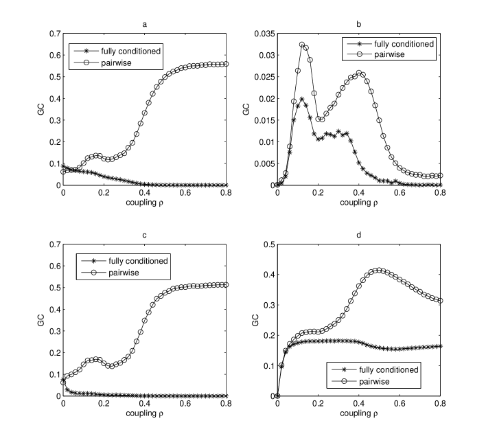
Figure 7: (a) The CGC and PWGC of the causal interaction $x_{1}\to x_{5}$ is plotted as a function of the coupling $\rho$ for the toy model for the proposed approach combining PWGC and CGC. The linear algorithms are used here and results are averaged over 100 runs of 2000 time points (b) The CGC and PWGC of the causal interaction between two variables in the multiplet is plotted as a function of the coupling $\rho$ for the toy model for the proposed approach combining PWGC and CGC. The linear algorithms are used here and results are averaged over 100 runs of 2000 time points (c) The nonlinear CGC and PWGC of the causal interaction $x_{1}\to x_{5}$ is plotted as a function of the coupling $\rho$ for the toy model for the proposed approach combining PWGC and CGC. The algorithm with the polynomial kernel of order 2 is used here and results are averaged over 100 runs of 2000 time points (d) The nonlinear CGC and PWGC of the causal interaction between two variables in the multiplet is plotted as a function of the coupling $\rho$ for the toy model for the proposed approach combining PWGC and CGC. The algorithm with the polynomial kernel of order 2 is used here and results are averaged over 100 runs of 2000 time points.

As a toy example to illustrate an application of the proposed approach, we consider a system made of five variables $\{x_{i}\}$. The first four constitute a multiplet made of an unidirectionally coupled logistic maps, eqs.(4-5) with $i$ ranging in $\{1,2,3,4\}$, coupling $\rho$ and interactions $1\to 2$, $2\to 3$ and $3\to 4$. The fifth variable is influenced by the mean field from the coupled map lattice, see equation (7). The four variables in the multiplet become almost synchronized for $\rho>0.4$. In figure 7 we depict both the average influence from the variables in the multiplet to $x_{5}$, and the average influence between pairs of variables in the multiplet: both linear and nonlinear PWGC and CGC are shown for the two quantities. Note that only the nonlinear algorithm correctly evidences the causal interactions within the multiplet of four variables, whilst the linear algorithm detects a very low causal interdependency among them. The driving influence from the multiplet to $x_{5}$ detected by CGC vanishes at high coupling redundancy, both in the linear and nonlinear approach, due to the redundancy induced by synchronization.

To explain how the proposed approach works we describe two situations, corresponding to low and high coupling. At low coupling, the CGC approach estimates the correct causal pattern in the system, and the nonzero elements of $\Delta$ are $1\to 2$, $2\to 3$, $3\to 4$, $1\to 5$, $2\to 5$, $3\to 5$ and $4\to 5$. The nonzero elements of the matrix $\Delta^{*}$, from PWGC analysis, are the same as $\Delta$ plus $1\to 3$, $1\to 4$, $2\to 4$, corresponding to indirect causalities; however these three interactions lead to non-zero elements of $\Delta^{2}$ (and, therefore, of $B$), hence they must be discarded. It follows that $\Delta^{*}$ does not provide further information than $\Delta$ at low coupling.

On the contrary at high coupling, due to synchronization, the CGC approach does not reveal the causal interactions $1\to 5$, $2\to 5$, $3\to 5$ and $4\to 5$, whilst still they are recognized by PWGC; $\Delta^{*}$ is still nonzero in correspondence of $1\to 5$, $2\to 5$, $3\to 5$ and $4\to 5$, while the corresponding elements of $B$ are vanishing. According to our previous discussion, the interactions $1\to 5$, $2\to 5$, $3\to 5$ and $4\to 5$, detected by PWGC, should not be discarded: combining the results by CGC and PWGC we obtain the correct causal pattern even in presence of strong synchronization.

VI Application to gene expression data.

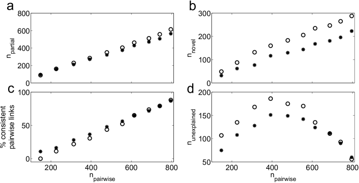
Figure 8: Concerning the genetic application, several quantities are plotted as a function of the number of bivariate causality links exceeding the threshold. (a) The number of retrieved links by PCGC with strategies IB ($\ast$) and PB (o). (b) The number of retrieved links by PCGC, with strategies IB ($\ast$) and PB (o), which are not present in the bivariate pattern. (c) The percentage of retrieved links, by BVGC, which are consistent with the PCGC with strategies IB ($\ast$) and PB (o). (d) The number of retrieved links by BVGC, which are not consistent with PCGC ( with strategies IB ($\ast$) and PB (o)).

HeLa hela is a famous cell culture, isolated from a human uterine cervical carcinoma in 1951. HeLa cells have acquired cellular immortality, in that the normal mechanisms of programmed cell death after a certain number of divisions have somehow been switched off. We consider the HeLa cell gene expression data of fujita . Data corresponds to $94$ genes and $48$ time points, with an hour interval separating two successive readings (the HeLa cell cycle lasts 16 hours). The 94 genes were selected from the full data set described in whitfield , on the basis of the association with cell cycle regulation and tumor development. We apply linear PWGC and linear CGC (using just another conditioning variable, and using both the selection strategies IB and PB described in Section III). We remark that the CGC approach is unfeasible in this case due to the limited number of samples. Due to the limited number of samples, in this case we do not use statistical testing for assessing the significance of the retrieved links, rather we introduce a threshold for the influence and analyze the pattern as the threshold is varied. In figure 8 results are reported as a function of the number of links found by PWGC $n_{pairwise}$ (which increases as the threshold is decreased); we plot (1) the number of links found by PGC $n_{partial}$, (2) the number of links found by PGC and not by PWGC $n_{novel}$, which are thus a signature of synergy, (3) the percentage of pairwise links which can be explained as direct or indirect causalities of the PGC pattern (thus being consistent with the partial causality pattern), found using the matrix $B_{1}$ to detect the indirect links, which correspond to circuits like the one described in figure 6a, (4) the number of causality links found by PWGC and not consistent with PWGC $n_{unexplained}$, corresponding to redundancy. The two curves refers to the two selection strategies for partial conditioning.

The low number of samples here allowed us just to use one conditioning variable, and therefore to analyze only circuits of three variables; a closely related analysis, see mindy , has been proposed to study how a gene modulates the interaction between two other genes. On the other hand, the true underlying gene regulatory network being unknown, we cannot assess the performances of the algorithms in terms of correctly detected links.

We note that both $n_{novel}$ and $n_{unexplained}$ assume relatively large values, hence both redundancy and synergy characterize this data-set. The selection strategy PB yields slightly higher values of $n_{novel}$ and $n_{unexplained}$, emerging then as a better discriminator of synergy and redundancy than IB. A comparison iwth the fully conditioned approach is not possible in this case. On the other hand, as far as the search for synergetic effects is concerned, we find that the synergetic interactions found by PCGC with the two strategies are not coinciding, indeed only $10\%$ of all the synergetic interactions are found by both strategies. This suggests that when searching for suppressors, several sets of conditioning variables should be used in CGC in order to explore more possible alternative pathways, especially when there is not a priori information on the network structure.

VII Conclusions

In this paper we have considered the inference, from time series data, of the information flow between subsystems of a complex network, an important problem in medicine and biology. In particular we have analyzed the effects that synergy and redundancy induce on the Granger causal analysis of time series.

Concerning synergy, we have shown that the search for synergetic contributions in the information flow is equivalent to the search for suppressors, i.e. variables that improve the predictive validity of another variable. Pairwise analysis fails to put in evidence this kind of variables; fully multivariate Granger causality solves this problem: conditioning on suppressors variables leads to nonzero Granger causality. In cases when the number of samples is low, we have shown that partially conditioned Granger causality is a valuable option, provided that the selection strategy, to choose the conditioning variables, succeeds in picking the suppressors. In this paper we have considered two different strategies: choosing the most informative variables for the candidate driver node, or choosing the nodes with the highest pairwise influence to the target. From the several examples analyzed here we have shown that the first strategy is viable in presence of redundancy, whilst when the interaction pattern has a tree-like structure, the latter is preferable; however the issue of selecting variables for partially conditioned Granger causality deserves further attention as it corresponds to the search for suppressor variables and correspondingly of synergetic effects. We have also provided evidence, for the first time, that synergetic effects are present in an epileptic brain in the preictal condition (just before the seizure).

We have then shown that fully conditioned Granger approaches do not work well in presence of redundancy. To handle redundancy, we propose to split the pairwise links in two subsets: those which correspond to indirect connections of the multivariate Granger causality, and those which are not. The links that are not explained as indirect connections are ascribed to redundancy effects and they are merged to those from CGC to provide the full causality pattern in the system. We have applied this approach to a genetic data-set from the HeLa culture, and found that the underlying gene regulatory networks are characterized by both redundancy and synergy, hence these approaches are promising also w.r.t. the reverse engineering of gene regulatory networks.

In conclusion, we observe that the problem of inferring reliable estimates of the causal interactions in real dynamical complex systems, when limited a priori information is available, remains a major theoretical challenge. In the last years the most important results in this direction are related to the use of data-driven approaches like Granger causality and transfer entropy. In this work we have shown that in presence of redundancy and synergy, combining the results from the pairwise and conditioned approaches may lead to more effective analyses.

References

- (1) A. Bashan, R.P. Bartsch, J. W. Kantelhardt, S. Havlin, P. Ch. Ivanov, Nature Communications 3, 702, (2012)
- (2) A.L. Barabasi, Linked: the new science of networks. (Perseus Publishing, Cambridge Mass., 2002); S. Boccaletti, V. Latora, Y. Moreno, M. Chavez and D.-U. Hwang, Phys. Rep. 424, 175 (2006).
- (3) L.F. Abbott, C. van Vreeswijk, Phys. Rev. E 48, 1483 (1993).
- (4) T.S. Gardner, D. Bernardo, D. Lorenz, J.J. Collins, Science 301, 102 (2003).
- (5) C.L. Tucker, J.F. Gera, P. Uetz, Trends Cell Biol. 11, 102 (2001).
- (6) H. Jeong, B. Tombor, R. Albert, Z.N. Oltvai, A.L. Barabasi, Nature 407, 651 (2000).
- (7) R. Guimerà, L.A. Nunes Amaral, Nature 433, 895 (2005)
- (8) IM De la Fuente, JM Cortes, MB Perez-Pinilla, V Ruiz-Rodriguez and J Veguillas, PLoS One 6, e27224 (2011)
- (9) E. Pereda, R. Quiroga, J. Bhattacharya, Progress in Neurobiology 77, 1 (2005)
- (10) M. Wibral, R. Vicente and J.T. Lizier (Eds.) Directed Information Measures in Neuroscience (Springer, Berlin, 2014);
- (11) K. Sameshima, L.A. Baccala (Eds.) Methods in Brain Connectivity Inference through Multivariate Time Series Analysis (CRC press, 2014);
- (12) C.W.J. Granger, Econometrica 37, 424 (1969).
- (13) S.L. Bressler, A.K. Seth, Neuroimage 58, 323 (2011)
- (14) T. Schreiber, Phys. Rev. Lett. 85, 461 (2000).
- (15) L. Barnett, A. B. Barrett, and A. K. Seth, Phys. Rev. Lett., vol. 103, no. 23, 2009.
- (16) K. Hlavackova-Schindler, Applied Mathematical Sciences 5, 3637 (2011)
- (17) R. Vicente, M. Wibral, M. Lindner, G. Pipa, J Comput Neurosci 30, 45 (2011)
- (18) D. Zhou, Y. Zhang, Y. Xiao and D. Cai, New J. Phys. 16, 043016 (2014)
- (19) R. P. Bartsch, P. Ch. Ivanov, Communications in Computer and Information Science, 438, pp 270-287 (2014)
- (20) R. P. Bartsch, A. Y. Schumann, J. W. Kantelhardtd, T. Penzele, and P. Ch. Ivanov, Proceedings of the National Academy of Sciences 109 (26), 10181-10186 (2012)
- (21) T. Ge, Y. Cui, W. Lin, J. Kurths and C. Liu, New J. Phys. 14 083028 (2012)
- (22) J. F. Geweke, Journal of the American Statistical Association, vol. 79, no. 388, pp. 907-915, 1984.
- (23) D. Marinazzo, M. Pellicoro, and S. Stramaglia, Computational and Mathematical Methods in Medicine, Volume 2012 (2012), Article ID 303601.
- (24) G. Wu, W. Liao, H. Chen, S. Stramaglia, D. Marinazzo Brain Connectivity, 3(3): 294-301 (2013)
- (25) L. Angelini et al., Phys. Rev. E 81, 037201 (2010).
- (26) V. Griffith and C. Koch, (2014). Quantifying synergistic mutual information, in Guided Self-Organization: Inception, Vol. 9, ed. M. Prokopenko (Berlin: Springer), 159 190.
- (27) M. Harder, C. Salge and D. Polani, Phys. Rev. E 87, 012130 (2013)
- (28) J.T. Lizier, B. Flecker, P.L. Williams Artificial Life (ALIFE), 2013 IEEE Symposium on , pp.43,51, doi: 10.1109/ALIFE.2013.6602430 (2013)
- (29) S. Yang, J. Gu, Jour of Zhejiang University Science 5, 1382 (2004)
- (30) E. Schneideman, W. Bialek, M.J. Berry, J Neurosci 23, 11539 (2003)
- (31) I. Gat and N. Tishby, NIPS page 111-117, the MIT press (1998).
- (32) A. B. Barrett, L. Barnett, and A. K. Seth, Phys.Rev. E, vol. 81, no. 4, Article ID 041907, 14 pages, 2010.
- (33) Z. Zhou, Y. Chen, M. Ding, P. Wright, Z. Lu, and Y. Liu, Human Brain Mapping, vol. 30, no. 7, pp. 2197 (2009)
- (34) D. Marinazzo, W. Liao, M. Pellicoro, and S. Stramaglia, Physics Letters, Section A, vol. 374, no. 39, pp. 4040 (2010)
- (35) AJ Conger, Educational and Psychological Measurement April 1974 vol. 34 no. 1 35-46
- (36) FT Thompson, DU Levine, Multiple Linear Regression Viewpoints, 24: 11 - 13 (1997)
- (37) S. Stramaglia, G. Wu, M. Pellicoro, D. Marinazzo Physical Review E, 86, 066211 (2012)
- (38) D. Chicharro, A. Ledberg Physical Review E, 86, 041901 (2012)
- (39) K. Hlavackova-Schindler, M. Palus, M. Vejmelka, J. Bhattacharya, Physics Reports 441, 1 (2007).
- (40) D. Marinazzo, M. Pellicoro and S. Stramaglia, Phys. Rev. E 77, 056215 (2008).
- (41) V. Vapnik. The Nature of Statistical Learning Theory. Springer, N.Y., 1995.
- (42) J. Shawe-Taylor and N. Cristianini, Kernel Methods For Pattern Analysis. (Cambridge University Press, London, 2004)
- (43) D. Marinazzo, M. Pellicoro, S. Stramaglia, Phys. Rev. Lett. 100, 144103 (2008).
- (44) N. Ancona and S. Stramaglia, Neural Comput. 18, 749 (2006).
- (45) http://math.bu.edu/people/kolaczyk/datasets.html, accessed may 2012
- (46) M.A. Kramer, E.D. Kolaczyk, H.E. Kirsch, Epilepsy Research 79, 173, 2008
- (47) J.R. Masters, Nature Reviews Cancer 2, 315 (2002).
- (48) A. Fujita et al., BMC System Biology 1:39, 1 (2007).
- (49) M.L. Whitfield et al., Mol. Biol. Cell 13, 1977 (2002).
- (50) K. Wang, et al. Nature Biotechnology 27, 829–837 (2009) doi:10.1038/nbt.1563