Unconfused Ultraconservative Multiclass Algorithms

Abstract

We tackle the problem of learning linear classifiers from noisy datasets in a multiclass setting. The two-class version of this problem was studied a few years ago by, e.g. Bylander (1994) and Blum et al. (1996): in these contributions, the proposed approaches to fight the noise revolve around a Perceptron learning scheme fed with peculiar examples computed through a weighted average of points from the noisy training set. We propose to build upon these approaches and we introduce a new algorithm called UMA (for Unconfused Multiclass additive Algorithm) which may be seen as a generalization to the multiclass setting of the previous approaches. In order to characterize the noise we use the confusion matrix as a multiclass extension of the classification noise studied in the aforementioned literature. Theoretically well-founded, UMA furthermore displays very good empirical noise robustness, as evidenced by numerical simulations conducted on both synthetic and real data.

1 Introduction

Context.

This paper deals with linear multiclass classification problems defined on an input space $\mathcal{X}$ (e.g., $\mathcal{X}=\mathbb{R}^{d}$) and a set of classes

$${\cal Q}\doteq\{1,\ldots Q\}.$$

In particular, we are interested in establishing the robustness of ultraconservative additive algorithms (Crammer and Singer, 2003) to label noise classification in the multiclass setting —in order to lighten notation, we will now refer to these algorithms as ultraconservative algorithms. We study whether it is possible to learn a linear predictor from a training set

$$\mathcal{S}\doteq\{(\bm{x}_{i},y_{i})\}_{i=1}^{n}$$

where $y_{i}\in{\cal Q}$ is a corrupted version of a true, i.e. deterministically computed class, $t(\bm{x}_{i})\in{\cal Q}$ associated with $\bm{x}_{i}$, according to some concept $t$. The random noise process $Y$ that corrupts the label to provides the $y_{i}$’s given the $\bm{x}_{i}$’s is fully described by a confusion matrix ${\cal C}=({\cal C}_{pq})_{p,q}\in\mathbb{R}^{Q\times Q}$ so that

$$\forall\bm{x},\;\mathbb{P}_{Y}(Y=p|\bm{x})={\cal C}_{pt(\bm{x})}.$$

The goal that we would like to achieve is to provide a learning procedure able to deal with the confusion noise present in the training set $\mathcal{S}$ to give rise to a classifier $h$ with small risk $\mathbb{P}_{X\sim D}(h(X)\neq t(X))$ —$D$ being the distribution of the $\bm{x}_{i}$’s. As we want to recover from the confusion noise, we use the term unconfused to characterize the procedures we propose.

Crammer and Singer (2003) introduce ultraconservative online learning algorithms, which output multiclass linear predictors of the form

$$f(\bm{x})=\operatorname*{\text{argmax}}_{r}\langle\bm{w}_{r},\bm{x}\rangle.$$

When processing a training pair $(\bm{x},y)$, these procedures perform updates of the form

$$\bm{w}_{q}^{\text{new}}\leftarrow\bm{w}_{q}+\tau_{q}\bm{x},\;q=1,\ldots Q,$$

so that:

• if $y=\operatorname*{\text{argmax}}_{q}\langle\bm{w}_{q},\bm{x}\rangle$, then $\tau_{1}=\cdots=\tau_{Q}=0$ (no update is made);

• otherwise (i.e. $y\neq\operatorname*{\text{argmax}}_{q}\langle\bm{w}_{q},\bm{x}\rangle$), then, given ${\cal E}\doteq\{r:r\neq y,\langle\bm{w}_{r},\bm{x}\rangle\geq\langle\bm{w}_{y},\bm{x}\rangle\}$, the $\tau_{q}$’s verify: a) $\tau_{y}=1$, b) $\forall q\in{\cal E},\tau_{q}\leq 0$, c) $\forall q\not\in\mathcal{E}\operatorname*{\cup}\{y\},\tau_{q}=0$, and d) $\sum_{q}^{Q}\tau_{q}=0$.

Ultraconservative learning procedures, have very nice theoretical properties regarding their convergence in the case of linearly separable datasets, provided a sufficient separation margin is guaranteed (as formalized in Assumption 1 below). In turn, these convergence-related properties yield generalization guarantees about the quality of the predictor learned. We build upon these nice convergence properties to show that ultraconservative algorithms are robust to a confusion noise process, provided an access to the confusion matrix ${\cal C}$ is granted and this paper is essentially devoted to proving how/why ultraconservative multiclass algorithms are indeed robust to such situations. To some extent, the results provided in the present contribution may be viewed as a generalization of the contributions on learning binary perceptrons under misclassification noise (Blum et al., 1996; Bylander, 1994).

Besides the theoretical questions raised by the learning setting considered, we may depict the following example of an actual learning scenario where learning from noisy data is relevant. This learning scenario will be further investigated from an empirical standpoint in the section devoted to numerical simulations (Section 4).

Example 1.1.

One situation where coping with mislabelled data is required arises in scenarios where labelling data is very expensive. Imagine a task of text categorization from a training set $\mathcal{S}=\mathcal{S}_{\ell}\operatorname*{\cup}\mathcal{S}_{u}$, where $\mathcal{S}_{\ell}=\{(\bm{x}_{i},y_{i})\}_{i=1}^{n}$ is a set of $n$ labelled training examples and $\mathcal{S}_{u}=\{\bm{x}_{n+i}\}_{i=1}^{m}$ is a set of $m$ unlabelled vectors; in order to fall back to a realistic training scenario, we may assume that $n<<m$. A possible three-stage strategy to learn a predictor is as follows: first learn a predictor $f_{\ell}$ on $\mathcal{S}_{\ell}$ and estimate its confusion ${\cal C}$ error via a cross-validation procedure, second, use the learned predictor to label all the data in $\mathcal{S}_{u}$ to produce the labelled traning set $\widehat{\mathcal{S}}=\{(\bm{x}_{n+i},t_{n+i}:=f(\bm{x}_{n+i}))\}_{i=1}^{m}$ and finally, learn a classifier $f$ from $\widehat{\mathcal{S}}$ and the confusion information ${\cal C}$.

Contributions

Our main contribution is to show that it is both practically and theoretically possible to learn a multiclass classifier on noisy data as long as some information on the noise process is available. We propose a way to compute update vectors for any ultraconservative algorithm which allows us to handle massive amount of mislabeled data without consequent loss of accuracy. Moreover, we provide a thorough analysis of our method and show that the strong theoretical guarantees that caracterize the family of ultraconservative algorithm carry over to the noisy scenario.

Organization of the paper.

Section 2 formally states the setting we consider throughout this paper. Section 3 provides the details of our main contribution: the UMA algorithm. Section 4 presents numerical simulation that support the soundness of our approach.

2 Setting and Problem

2.1 Noisy Labels with Underlying Linear Concept

The probabilistic setting we consider hinges on the existence of two components. On the one hand, we assume an unknown (but fixed) probability distribution $\mathcal{D}$ on the intput space $\mathcal{X}\doteq\mathbb{R}^{d}$; without loss of generality, we suppose that $\mathbb{P}_{X\sim\mathcal{D}}(\|X\|=1)=1$, where $\|\cdot\|$ is the Euclidean norm. On the other hand, we also assume the existence of a deterministic labelling function $t:\mathcal{X}\to{\cal Q}$, where ${\cal Q}\doteq\{1,\ldots Q\}$, which associates a label $t(\bm{x})$ to any input example $\bm{x}$; in the Probably Approximately Correct literature, $t$ is sometimes referred to as a concept (Kearns and Vazirani, 1994; Valiant, 1984). Throughout, we assume the following:

Assumption 1 (Linear Separability with $\theta$ Margin.)

Concept $t$ is such that there exists a compatible linear classifier $f^{*}$ with margin $\theta>0$. This means that

$$\mathbb{P}_{X\sim\mathcal{D}}(f^{*}(X)\neq t(X))=0, f^{*} t$$ (comptability of wrt )

and there exist $\theta>0$ and $W^{*}=[\bm{w}_{1}^{*}\cdots\bm{w}_{Q}^{*}]\in\mathbb{R}^{d\times Q}$ such that

$$\forall\bm{x}\in\mathcal{X},\;f^{*}(\bm{x})=\operatorname*{\text{argmax}}\nolimits_{q\in{\cal Q}}\langle\bm{w}_{q},\bm{x}\rangle, f^{*}$$ ( is a linear classifier)

$$\mathbb{P}_{X\sim\mathcal{D}}\left\{\exists p\neq t(X):\left\langle\bm{w}^{*}_{t(X)}-\bm{w}^{*}_{p},X\right\rangle\leq\theta\right\}=0. f^{*} \theta t \mathcal{D}$$ ( has margin wrt and )

(Here, $\langle\cdot,\cdot\rangle$ denotes the canonical inner product of $\mathbb{R}^{d}$.)

In a usual setting, one would be asked to learn a classifier $f$ from a training set

$$\mathcal{S}_{\text{true}}\doteq\{(\bm{x}_{i},t(\bm{x}_{i})\}_{i=1}^{n}$$

made of $n$ labelled pairs from $\mathcal{X}\times{\cal Q}$ such that the $\bm{x}_{i}$’s are independent realizations of a random variable $X$ distributed according to $\mathcal{D}$, with the objective of minimizing the true risk or misclassification error $R_{\text{error}}(f)$ of $f$ given by

$$R_{\text{error}}(f)\doteq\mathbb{P}_{X\sim\mathcal{D}}(f(X)\neq t(X)).$$ (1)

In other words, the objective is for $f$ to have a prediction behavior as close as possible to that of $t$.

As announced in the introduction, there is a little twist in the problem that we are going to tackle. Instead of having direct access to $\mathcal{S}_{\text{true}}$, we assume that we only have access to a corrupted version

$$\mathcal{S}\doteq\{(\bm{x}_{i},y_{i})\}_{i=1}^{n}$$ (2)

where each $y_{i}$ is the realization of a random variable $Y$ whose law $\mathcal{D}_{Y|X}$ (which is conditioned on $X$) is so that the conditional distribution $\mathbb{P}_{Y\sim\mathcal{D}_{Y|X=\bm{x}}}(Y|X=\bm{x})$ is fully summarized into a known confusion matrix ${\cal C}$ given by

$$\forall\bm{x},\;{\cal C}_{pt(\bm{x})}\doteq\mathbb{P}_{Y\sim\mathcal{D}_{Y|X=\bm{x}}}(Y=p|X=\bm{x})=\mathbb{P}_{Y\sim\mathcal{D}_{Y|X=\bm{x}}}(Y=p|t(\bm{x})=q).$$ (3)

Henceforth, the noise process that corrupts the data is uniform within each class and its level does not depend on the precise location of $\bm{x}$ within the region that corresponds to class $t(\bm{x})$. Noise process $Y$ is both very aggressive, as it does not only apply, as we may expect, to regions close to the boundaries between classes and very regular, as the mislabelling rate is piecewise constant.

The setting we assume allows us to view $\mathcal{S}$ as the realization of a random sample $\{(X_{i},Y_{i})\}_{i=1}^{n}$, where each pair $(X_{i},Y_{i})$ is an independent copy of the random pair $(X,Y)$ of law $\mathcal{D}_{XY}\doteq\mathcal{D}_{X}\mathcal{D}_{X|Y}.$

2.2 Problem: Learning a Linear Classifier from Noisy Data

The problem we address is the learning of a classifier $f$ from $\mathcal{S}$ and ${\cal C}$ so that the error rate

$$R_{\text{error}}(f)=\mathbb{P}_{X\sim\mathcal{D}}(f(X)\neq t(X))$$

of $f$, is as small as possible: the usual goal of learning a classifiier $f$ with small risk is preserved, while now the training data is only made of corrupted labelled pairs.

Building on Assumption 1, we may refine our learning objective by restricting ourselves to linear classifiers $f_{W}$, for $W=[\bm{w}_{1}\cdots\bm{w}_{Q}]\in\mathbb{R}^{d\times Q}$ such that

$$\forall\bm{x}\in\mathcal{X},\;f_{W}(\bm{x})\doteq\operatorname*{\text{argmax}}\nolimits_{q\in{\cal Q}}\langle\bm{w}_{q},\bm{x}\rangle,$$ (4)

and our goal is thus to learn a relevant matrix $W$ from $\mathcal{S}$ and the confusion information ${\cal C}$.

3 Uma: Unconfused Ultraconservative Multiclass Algorithm

3.1 Main Result and High Level Justification

This section presents our main contribution, UMA, a theoretically grounded noise-tolerant multiclass algorithm depicted in Algorithm 1. UMA learns and outputs a matrix $W=[\bm{w}_{1}\cdots\bm{w}_{Q}]\in\mathbb{R}^{d\times Q}$ from a noisy training set $\mathcal{S}$ to produce the associated classifier

$$f_{W}(\cdot)=\operatorname*{\text{argmax}}_{q}\langle\bm{w}_{q},\cdot\rangle$$ (5)

by iteratively updating the $\bm{w}_{q}$’s, whilst maintaining $\sum_{q}\bm{w}_{q}=0$ throughout the learning process. We may already recognize the generic step sizes promoted by ultraconservative algorithms in step 8 and step 9 of the algorithm (Crammer and Singer, 2003). An important feature of UMA is that it only uses information provided by $\mathcal{S}$ and does not make assumption on the accessibility to the noise-free dataset $\mathcal{S}_{\text{true}}$.

Algorithm 1 UMA: Unconfused Ultraconservative Multiclass Algorithm

0:  $\mathcal{S}=\{(\bm{x}_{i},y_{i})\}_{i=1}^{n}$, ${\cal C}\in\mathbb{R}^{Q\times Q}$, confusion matrix and $\alpha>0$

0:  $W=\left[\bm{w}_{1},\ldots,\bm{w}_{K}\right]$ and classifier $f_{W}(\cdot)=\operatorname*{\text{argmax}}_{q}\langle\bm{w}_{q},\cdot\rangle$

1:  $\bm{w}_{k}\leftarrow 0$, $\forall k\in{\cal Q}$

2:  repeat

3:     select $p$ and $q$

4:     $\mathcal{A}_{p}^{\alpha}\leftarrow\left\{\bm{x}|\bm{x}\in\mathcal{S}\wedge\left<{\bm{w}_{p}},{\bm{x}}\right>-\left<{\bm{w}_{k}},{\bm{x}}\right>>\alpha,\;\forall k\neq p\right\}$

5:     $\gamma_{k}^{p}\leftarrow\frac{1}{n}\sum_{i:y_{i}=k\wedge\bm{x}_{i}\in\mathcal{A}_{p}^{\alpha}}\bm{x}_{i}^{\top}$, $\forall k\in{\cal Q}$

6:     form $\Gamma^{p}\in\mathbb{R}^{Q\times d}$ as  $\Gamma^{p}\leftarrow\left[\begin{array}[]{c}\gamma_{1}^{p}\\ \vdots\\ \gamma_{Q}^{p}\end{array}\right],$

7:     compute the update vector $\bm{z}_{pq}$ according to  ${\bm{z}}_{pq}\leftarrow([{\cal C}^{-1}\Gamma^{p}]_{q})^{\top}$, (where $[A]_{q}$ refers to the $q$th row of matrix $A$)

8:     compute the error set  ${\cal E}^{\alpha}\leftarrow\{r\in{\cal Q}:r\neq q,\langle\bm{w}_{r},\bm{z}_{pq}\rangle-\langle\bm{w}_{q},\bm{z}_{pq}\rangle\geq\alpha\}$

9:     compute some ultraconservative update steps $\tau_{1},\ldots,\tau_{Q}$ such that:   $\sum_{r=1}^{Q}\tau_{r}=0$ and $\left\{\begin{array}[]{l}\tau_{q}=1\\ \tau_{r}\leq 0,\forall r\in{\cal E}^{\alpha}\\ \tau_{r}=0,\text{ otherwise}\end{array}\right.$

10:     perform the updates  $\bm{w}_{r}\leftarrow\bm{w}_{r}+\tau_{r}\bm{z}_{pq}$

11:  until $\|{\bf z}_{pq}\|$ is too small

Establishing that under some conditions UMA stops and provides a classifier with small risk is the purpose of the following subsections; we will also discuss the unspecified step 3, dealing with the selection step.

For the impatient reader, we may already leak some of the ingredients we use to prove the relevance of our procedure. The pivotal result regarding the convergence of ultraconservative algorithms is ultimately a generalized Block-Novikoff theorem (Crammer and Singer, 2003; Minsky and Papert, 1969), which rests on the analysis of the updates made when training examples are misclassified by the current classifier. If the training problem is linearly separable with a positive margin, then the number of updates/mistakes can be (easily) bounded, which establishes the convergence of the algorithms. The conveyed message is therefore that examples that are erred upon are central to the convergence analysis. It turns out that step 4 through 7 of UMA (cf. Algorithm 1) construct, with high probabilty, a point $\bm{z}_{pq}$ that is mistaken on. More precisely, the true class $t(\bm{z}_{pq})$ of $\bm{z}_{pq}$ is $q$ and it is predicted to be of class $p$ by the current classifier; at the same time, these update vectors are guaranteed to realize a positive margin condition with respect to $W^{*}$: $\langle\bm{w}_{q}^{*},\bm{z}_{pq}\rangle>\langle\bm{w}_{k}^{*},\bm{z}_{pq}\rangle$ for all $k\neq q$. The ultraconservative feature of the algorithm is carried by step 8 and step 9, which make it possible to update any prototype vector $\bm{w}_{r}$ with $r\neq q$ having an inner product $\langle\bm{w}_{r},{\bf z}_{pq}\rangle$ with ${\bf z}_{pq}$ larger than $\langle\bm{w}_{q},{\bf z}_{pq}\rangle$ (which should be the largest if a correct prediction were made). The reason why we have results ‘with high probability’ is because the $z_{pq}$’s are (sample-based) estimates of update vectors known to be of class $q$ but predicted as being of class $p$, with $p\neq q$; computing the accuracy of the sample estimates is one of the important exercises of what follows. A control on the accuracy makes it possible for us to then establish the convergence of the proposed algorithm. In order to ease the analysis we conduct, we assume the following.

Assumption 2

From now on, we make the assumption that ${\cal C}$ is invertible. Investigating learnability under a milder constraint is something that goes beyond the scope of the present paper and that we left for future work.

From a practical standpoint, it is worth noticing that there are many situations where the confusion matrices are diagonally dominant, therefore invertible.

3.2 ${\bf z}_{pq}$ is Probably a Mistake with Positive Margin

Here, we prove that the update vector $\bm{z}_{pq}$ given in step 7 is, with high probability, a point on which the current classifier errs.

Proposition 3.1.

Let $W=[\bm{w}_{1}\cdots\bm{w}_{Q}]\in\mathbb{R}^{d\times Q}$ and $\alpha\geq 0$ be fixed. Let $\mathcal{A}_{p}^{\alpha}$ be defined as in step 4 of Algorithm 1, i.e:

$$\mathcal{A}_{p}^{\alpha}\doteq\left\{\bm{x}|\bm{x}\in\mathcal{S}\wedge\left<{\bm{w}_{p}},{\bm{x}}\right>-\left<{\bm{w}_{k}},{\bm{x}}\right>>\alpha,\;\forall k\neq p\right\}.$$ (6)

For $k\in{\cal Q}$, $p\neq k$, consider the random variable $\gamma_{k}^{p}$:

$$\gamma_{k}^{p}\doteq\frac{1}{n}\sum_{i}\mathbb{I}{\left\{Y_{i}=k\right\}}\mathbb{I}{\left\{X_{i}\in\mathcal{A}_{p}^{\alpha}\right\}}X_{i}^{\top},$$

($\gamma_{k}^{p}$ of step 5 of Algorithm 1 is a realization of this variable, hence the overloading of notation $\gamma_{k}^{p}$).

The following holds, for all $k\in{\cal Q}$:

$$\mathbb{E}_{\mathcal{S}}\left\{\gamma_{k}^{p}\right\}=\mathbb{E}_{\{(X_{i},Y_{i})\}_{i=1}^{n}}\left\{\gamma_{k}^{p}\right\}=\sum_{q=1}^{Q}{\cal C}_{kq}\mu_{q}^{p},$$ (7)

where

$$\mu_{q}^{p}\doteq\mathbb{E}_{X}\left\{\mathbb{I}{\left\{t(X)=q\right\}}\mathbb{I}{\left\{X\in\mathcal{A}_{p}^{\alpha}\right\}}X^{\top}\right\}.$$ (8)

Proof 3.2.

Let us compute $\mathbb{E}_{XY}\{\mathbb{I}{\left\{Y=k\right\}}\mathbb{I}{\left\{X\in\mathcal{A}_{p}^{\alpha}\right\}}X^{\top}\}$: ΔE_XY{I{ Y=k } I{ X∈A_p^α } X^⊤}&=∫_X∑_q=1^QI{ q=k } I{ x∈A_p^α } x^⊤P_Y(Y=q—X=x)dD_X(x)
=∫_XI{ x∈A_p^α } x^⊤P_Y(Y=k—X=x)dD_X(x)
=∫_XI{ x∈A_p^α } x^⊤C_kt(x)dD_X(x)
=∫_X∑_q=1^QI{ t(x)=q } I{ x∈A_p^α } x^⊤C_kqdD_X(x)
=∑_q=1^Q C_kq∫_XI{ t(x)=q } I{ x∈A_p^α } x^⊤dD_X(x)=∑_q=1^Q C_kqμ_q^p, where the next-to-last line comes from the fact that the classes are non-overlapping. The fact that the $n$ pairs $(X_{i},Y_{i})$ are identically and independently distributed give the result.

Intuitively, $\mu_{q}^{p}$ must be seen as an example of class $p$ which is erroneously predicted as being of class $q$. Such an example is precisely what we are looking for to update the current classifier; as expecations cannot be computed, the estimate $\bm{z}_{pq}$ of $\mu_{q}^{p}$ is used instead of $\mu_{q}^{p}$.

Proposition 3.3.

Let $W=[\bm{w}_{1}\cdots\bm{w}_{Q}]\in\mathbb{R}^{d\times Q}$ and $\alpha\geq 0$ be fixed. For $p,q\in{\cal Q}$, $p\neq q$, ${\bm{z}}_{pq}\in\mathbb{R}^{d}$ is such that

$$\mathbb{E}_{XY}{{\bm{z}}_{pq}}=\mu_{q}^{p}$$ (8)

$$\langle\bm{w}_{q}^{*},\mu_{q}^{p}\rangle-\langle\bm{w}_{k}^{*},\mu_{q}^{p}\rangle\geq\theta,\;\forall k\neq q,$$ (9)

$$\langle\bm{w}_{p},\mu_{q}^{p}\rangle-\langle\bm{w}_{k},\mu_{q}^{p}\rangle>\alpha,\;\forall k\neq p.$$ (10)

(Normally, we should consider the transpose of $\mu_{q}^{p}$, but since we deal with vectors of $\mathbb{R}^{d}$ —and not matrices— we omit the transpose for sake of readability.)

This means that

1. $t(\mu_{q}^{p})=q$, i.e. the ‘true’ class of $\mu_{q}^{p}$ is $q$;

2. and $f_{W}(\mu_{q}^{p})=p$: $\mu_{q}^{p}$ is therefore misclassified by the current classifier $f_{W}$.

Proof 3.4.

According to Proposition 3.1,

$$\mathbb{E}_{XY}\left\{\Gamma^{p}\right\}=\mathbb{E}_{XY}\left\{\left[\begin{array}[]{c}\gamma_{1}^{p}\\ \vdots\\ \gamma_{Q}^{p}\end{array}\right]\right\}=\left[\begin{array}[]{c}\mathbb{E}_{XY}\left\{\gamma_{1}^{p}\right\}\\ \vdots\\ \mathbb{E}_{XY}\left\{\gamma_{Q}^{p}\right\}\end{array}\right]=\left[\begin{array}[]{c}\sum_{q=1}^{Q}{\cal C}_{1q}\mu_{q}^{p}\\ \vdots\\ \sum_{q=1}^{Q}{\cal C}_{Qq}\mu_{q}^{p}\end{array}\right]={\cal C}\left[\begin{array}[]{c}\mu_{1}^{p}\\ \vdots\\ \mu_{Q}^{p}\end{array}\right].$$

Hence, inverting ${\cal C}$ and extracting the $q$th of the resulting matrix equality gives that $\mathbb{E}\left\{{\bm{z}}_{pq}\right\}=\mu_{q}^{p}$.

Equation (9) is obtained thanks to Assumption 1 combined with the linearity of the expectation. Equation (10) is obtained thanks to the definition (6) of $\mathcal{A}_{p}^{\alpha}$ (made of points that are predicted to be of class $p$) and the linearity of the expectation.

Proposition 3.5.

Let $\varepsilon>0$ and $\delta\in(0;1]$. There exists a number

$$n_{0}(\epsilon,\delta,d,Q)=O\left(\frac{1}{\epsilon^{2}}\left[\ln\frac{1}{\delta}+\ln Q+d\ln\frac{1}{\epsilon}\right]\right)$$

such that if the number of training samples is greater than $n_{0}$ then, with high probability

$$\langle\bm{w}_{q}^{*},\bm{z}_{pq}\rangle-\langle\bm{w}_{k}^{*},\bm{z}_{pq}\rangle\geq\theta-\epsilon$$ (11)

$$\langle\bm{w}_{p},\bm{z}_{pq}\rangle-\langle\bm{w}_{k},\bm{z}_{pq}\rangle\geq 0,\;\forall k\neq p.$$ (12)

Proof 3.6.

The existence of $n_{0}$ rely on pseudo-dimension arguments. We defer this part of the proof to Appendix A and we will directly assume here that if $n\geq n_{0}$, then, with probability $1-\delta$ :

$$|\left<{\bm{w}_{p}-\bm{w}_{q}},{\bm{z}_{pq}}\right>-\left<{\bm{w}_{p}-\bm{w}_{q}},{\mu_{q}^{p}}\right>|\leq\varepsilon$$ (13)

for any $\bm{W}$, $\bm{z}_{pq}$.

Proving (11) then proceed by observing that

$$\left<{\bm{w}_{q}^{*}-\bm{w}_{k}^{*}},{\bm{z}_{pq}}\right>=\left<{\bm{w}_{q}^{*}-\bm{w}_{k}^{*}},{\mu_{q}^{p}}\right>+\left<{\bm{w}_{q}^{*}-\bm{w}_{k}^{*}},{\bm{z}_{pq}-\mu_{q}^{p}}\right>$$

bounding the first part using Proposition $2$:

$$\left<{\bm{w}_{q}^{*}-\bm{w}_{k}^{*}},{\mu_{q}^{p}}\right>\geq\theta$$

and the second one with (13). A similar reasoning allows us to get (12) by setting $\alpha\doteq\varepsilon$ in $\mathcal{A}_{p}^{\alpha}$ .

This last proposition essentially says that the update vectors ${\bf z}_{pq}$ that we compute are, with high probability, erred upon and realize a margin condition $\theta/2.$

3.3 Convergence and Stopping Criterion

In order to arrive at the main result of our paper, we recall the following Theorem of Crammer and Singer (2003), which stated the convergence of general ultraconservative learning algorithms.

Theorem 3.7 (Crammer and Singer (2003)).

Let $\{({\bm{x}}_{i},t_{i})\}_{i=1}^{n}$ be a linearly separable sample such that there exists a separating linear classifier $W^{*}$ with margin $\theta$. Then any multiclass ultraconservative algorithm will make no more than $2/{\theta}^{2}$ updates before convergence.

We arrive at our main result, which provides both convergence and a stopping criterion.

Proposition 3.8.

There exists a number $n_{1}$, polynomial in $d,1/\widehat{\theta},Q,1/\delta$, such that is the training sample is of size at least $n_{1}$, then, with high probability ($1-\delta$), UMA makes at most $O(1/\widehat{\theta}^{2})$ iterations for all $p,q$.

Proof 3.9.

This results is obtained as a direct combination of Proposition 3.5 and Theorem 3.7, with the adjusted margin $\theta-\varepsilon$ It comes as in Blum et al. (1996) that the conditional misclassification errors $\mathbb{P}(f_{W}(X)=p|Y=q)$ are all small.

3.4 Selecting $p$ and $q$

So far, the question of selecting good pairs of values $p$ and $q$ to perform updates has been left unanswered. Intuitively, we would like to focus on the pair $(p,q)$ for which the instantaneous empirical misclassification rate is the highest. We want to privilege those pairs $(p,q)$ because, first the induced update will likely lead to a greater reduction of the error and then, and more importantly, because $\bm{z}_{pq}$ will be more reliable, as computed on larger samples of data. Another wise strategy for selecting $p$ and $q$ might be to select the pair $(p,q)$ for which the empirical probability $\hat{\mathbb{P}}(f_{W}(X)=p|Y=q)$ is the largest.

From these two strategies, we propose two possible computations for $(p,q)$:

$$(p,q)_{\text{error}}\doteq\arg\max_{(p,q)}\|{\bf z}_{pq}\|$$ (14)

$$(p,q)_{\text{conf}}\doteq\arg\max_{(p,q)}\frac{\|{\bf z}_{pq}\|}{\hat{\pi}_{q}}$$ (15)

where $\hat{\pi}_{q}$ is the estimated proportion of examples of true class $q$ in the training sample. In a way similar to the computation of ${\bf z}_{pq}$ in Algorithm 1, $\hat{\pi}_{q}$ may be computed as follows:

$$\hat{\pi}_{q}=\frac{1}{n}[{\cal C}^{-1}{\hat{\bm{y}}}]_{q},$$

where $\bm{y}\in\mathbb{R}^{Q}$ is the vector containing the number of examples from $\mathcal{S}$ having noisy labels $1,\ldots,Q$, respectively.

The second selection criterion is intended to normalize the number of errors with respect to the proportions of different classes and aims at being robust to imbalanced data.

4 Experiments

In this section, we present numerical results from empirical evaluations of our approach and we discuss different practical aspects of UMA. The ultraconservative step sizes retained are those corresponding to a regular Percepton, or, in short: $\tau_{p}=-1$ and $\tau_{q}=+1$.

Section 4.1 covers robustness results, based on simulations with synthetic data while Section 4.2 takes it a step further and evaluates our algorithm on real data, with a realistic noise process related to Example 1.1 (cf. Section ).

We essentially use the confusion rate as a performance measure, which is the Frobenius norm of the confusion matrix estimated on a test set $S_{\text{test}}$ (independent from the training set) and which is defined as:

$$\|{{\widehat{C}}}\|_{F}=\sqrt{\sum_{i,j}\widehat{C}_{ij}^{2}},\text{ with }\widehat{C}_{pq}=\frac{\sum_{\bm{x}_{i}\in S_{\text{test}}}\mathbb{I}{\left\{t_{i}=q\wedge\widehat{y}_{i}=q\right\}}}{\sum_{\bm{x}_{i}\in S_{\text{test}}}\mathbb{I}{\left\{t_{i}=q\right\}}},$$

where $\widehat{y}_{i}$ is the label predicted for test instance ${\bf x}_{i}$ by the learned predictor.

4.1 Toy dataset

We use a $10$-class dataset with a total of roughly $1,000$ $2$-dimensional examples uniformly distributed over the unit circle centered at the origin. Labelling is achieved according to (4), where each of the 10 $\bm{w}$ are randomly generated from the same distribution than the examples (uniformly over the unit circle centered at the origin). Then a margin $\theta=0.025$ is enforced by removing examples too close of the decision boundaries. Note that because of the way we generate them, all the normal vector $\bm{w}$ of each hyperplanes are normalized. This is to prevent the cases where the margin with respect to some given class is artificially high because of the norm of $\bm{w}$. Hence, all classes are guaranteed to be present in the training set as long as the margin constraint does not preclude it.

The learned classifiers are tested against a similarly generated dataset of $10,000$ points. The results reported in the tables are averaged over $10$ runs.

The noise is generated from the sole confusion matrix. This situation can be tough to handle and is rarely met with real data but we stick with it as it is a good example of a worst-case scenario.

We first evaluate the robustness to noise level (Fig. 1). We randomly generate a reference stochastic matrix $M$ and we define $N$ such that $M=I+10\times N$. Then we run UMA $20$ times with confusion matrix $C$ ranging from $N$ to $20N$. Figure 1 plots the confusion rate against $\|{{C}}\|_{F}$.

The second experiment (Fig. 1) evaluates the robustness to errors in the estimation of the noise. We proceed in a similar way as before, but the data are always corrupted according to $M$. The approximation factor of $C=i\times N$ is then defined as $1-i/10$. Figure 1 plots the confusion rate against this approximation factor. Note that an approximation factor of $1$ corresponds to the identity matrix and, in that case, UMA behaves as a regular Perceptron. More generally, the noise is underestimated when the approximation factor is positive, and overestimated when it is negative.

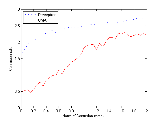
[Robustness to noise] [Robustness to noise estimation]

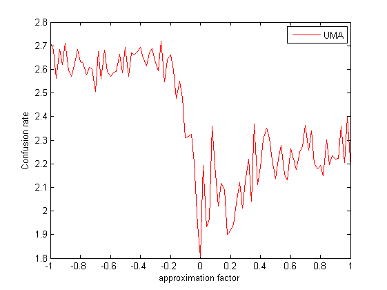
Figure 1: (a) evolution of the Confusion rate for different noise levels; (b) evolution of the same quantity with respect to errors in the confusion matrix $C$.

These first simulations show that UMA provides improvements over the Perceptron for every noise level tested —although its performance obviously slightly degrades as the noise level increases. The second simulation points out that, in addition to being robust to the noise process itself, UMA is also robust to underestimated noise levels, but not to overestimated ones.

4.2 Reuters

The Reuters dataset is a nearly linearly separable document categorization dataset. The training (resp. test) set is made of approximately $15,000$ (resp. $300,000$) examples in roughly $50,000$ dimensions spread over $50$ classes.

To put ourselves in a realistic learning scenario, we assume that labelling examples is very expensive and we implement the strategy evoked in Example 1.1 (cf. introduction). Thus, we label only $3$ percent (selected at random) of the training set. Our strategy is to learn a classifier over half of the labelled examples, and then to use the classifier to label the entire training set. This way, we end up with a labelled training set with noisy labels, since $1.5$ percent of the whole training set is evidently not sufficient to learn a reliable classifier. In order to gather the information needed by UMA to learn, we estimate the confusion matrix of the whole training set using the remaining 1.5% correctly labelled examples (i.e. those examples not used for learning the labelling classifier).

However, it occurs that some classes are so under-represented that they are flooded by the noise process and/or are not present in the original $1.5$ percent, which leads to a non-invertible confusion matrix. We therefore restrict the dataset to the $19$ largest classes. One might wonder whether doing so removes class imbalance. This is not the case as the least represented class accounts for $198$ examples while this number reaches $4,000$ for the most represented one. As in Section 4.1, the results reported are an average over 10 runs of the same experiment.

We use three variations of UMA with different strategies for selecting $(p,q)$ (error, confusion, and random) and monitor each one along the learning process.

We also compare UMA with the regular Perceptron in order to quantify the increase in accuracy induced by the use of the confusion matrix. We compare UMA with two different settings, one with the noisy classes (Mperc), and one with the true data (Mperc${}_{\text{full}}$).

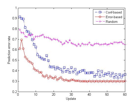
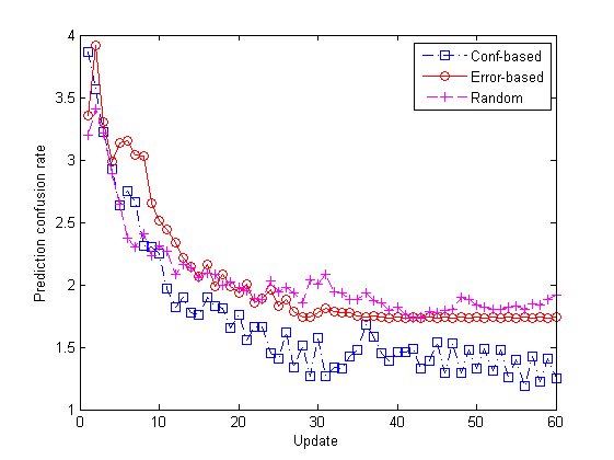
Figure 2: Error and confusion risk on Reuters dataset with various update strategies.

From Figure 2, we observe that both performance measures evolve similarly, attaining a stable state around the $30^{\text{th}}$ iteration. The best strategy depends of the performance measure used, even though it is noticeable the random strategy is alway non-optimal.

As one might expect, the confusion-based strategy performs better than the error-based one with respect to the confusion rate while the converse holds when considering the error rate. This observation motivates us to thoroughly study the confusion-based strategy in a near future.

The plateau reached around the $30^{\text{th}}$ may be puzzling, since the studied dataset presents no positive margin and convergence is therefore not guaranteed. However the non-existence of a linear separability can be also interpreted as label noise. Keeping this in mind, our current setup is equivalent to the one where noise is added after the estimation of the confusion matrix, thus leading to an underestimated confusion matrix. Nonetheless it is worth noting that, according to Figure 1, UMA is robust to this situation, which explains the good results exhibited.

Algorithm	M-perc	M-perc${}_{\text{full}}$	UMA
error rate	$0.482$	$0.379$	$0.381$

Table 1: Performances of different algorithms

Looking at the results, it is clear that UMA successfully recovers from the noise, attaining an error rate similar to the one attained with the uncorrupted data (cf. Table 1). However it is good to temper this result as Reuters is not linearly separable. We have already seen (Fig. 1, Figure 2) that this is not really a problem for UMA, unlike the regular multiclass Perceptron. Thus, the present setting, while providing a great practical setup, is somewhat biaised in favor of UMA.

Finally, note that the results of Section 4.2 are quite better than those of Section 4.1 . Indeed, in the Reuters experiment, the noise is concentrated around the decision boundaries because this is typically where the labelling classifier would make errors. This kind of noise is called monotonic noise and is a special, easier, case of classification noise as discussed in Bylander (1994).

5 conclusion

In this paper, we have proposed a new algorithm to cope with noisy examples in multiclass linear problems. This is, to the best of our knowledge, the first time the confusion matrix is used as a way to handle noisy label in multiclass problem. Moreover, UMA does not consist in a binary mapping of the original problem and therefore benefits from the good theoretical guarantees of additive algorithms. Besides, UMA can be adapted to a wide variety of additive algorithms, allowing to handle noise with multiple methods. On the sample complexity side, note that a more tight bound can be derived with specific multiclass tools as the Natarajan’s dimension (see Daniely et al. (2011) for example). However as it is not the core of this paper we stuck with the classic analysis here.

To complement this work, we want to investigate a way to properly tackle near-linear problems (as Reuters). As for now the algorithm already does a very good jobs thanks to its noise robustness. However more work has to be done to derive a proper way to handle case where a perfect classifier does not exists. We think there are great avenues for interesting research in this domain with an algorithm like UMA and we are curious to see how this present work may carry over to more general problems.

Appendix A Double sample theorem

Proof A.1 (Proposition 3.5).

For a fixed couple $(p,q)\in\mathcal{Y}^{2}$ we consider the family of functions

$$\mathcal{F}_{pq}\doteq\{f:f(\bm{x})\doteq\left<{\bm{w}_{p}-\bm{w}_{q}},{x}\right>:\bm{w}_{p},\bm{w}_{q}\in\mathbb{R}^{d}\}$$

with the corresponding loss function

$$l^{f}(\bm{x},y)\doteq l(f(\bm{x}),y)\doteq 1+f(\bm{x})$$

Clearly, $\mathcal{F}_{pq}$ is a subspace of affine functions, thus $\text{Pdim}(\mathcal{F}_{pq})\leq(n+1)$, where $\text{Pdim}(\mathcal{F}_{pq})$ is the pseudo-dimension of $\mathcal{F}_{pq}$. Additionally, $l$ is Lipschitz in its first argument with a Lipschitz factor of $L\doteq 1$ as $\forall y,y_{1},y_{2},\in\mathcal{Y}:|l(y_{1},y)-l(y_{2},y)|=|y_{1}-y_{2}|$

Let $\mathcal{D}_{pq}$ be any distribution over $\mathcal{X}\times\mathcal{Y}$ and $T\in(\mathcal{X}\times\mathcal{Y})^{m}$ such that $T\sim\mathcal{D}_{pq}^{m}$, then define the empirical loss $\text{err}_{T}^{l}[f]\doteq\frac{1}{m}\sum_{\bm{x}_{i}\in T}l(\bm{x}_{i},y_{i})$ and the expected loss $\text{err}_{\mathcal{D}}^{l}[f]\doteq\mathbb{E}_{\mathcal{D}}\left[l(\bm{x},y)\right]$

The goal here is to prove that

$$\mathbb{P}_{T\sim\mathcal{D}-{pq}^{m}}\left(\sup_{f\in\mathcal{F}_{pq}}|\text{err}_{\mathcal{D}}^{l}[f]-\text{err}_{T}^{l}[f]\geq\epsilon\right)\leq O\left(4\times\left(\frac{8}{\epsilon}\right)^{(d+1)}e^{{m\epsilon^{2}}/_{128}}\right)$$ (16)

Proof A.2 (Proof of (16)).

We start by noting that $l(y_{1},y_{2})\in[0,2]$ and then proceed with a classic $4$-step double sampling proof. Namely :

Symmetrization We introduce a ghost sample $T^{\prime}\in(\mathcal{X}\times\mathcal{Y})^{m}$, $T^{\prime}\sim\mathcal{D}_{pq}^{m}$ and show that for $f^{\text{bad}}_{T}$ such that $|\text{err}_{\mathcal{D}_{pq}}^{l}[f^{\text{bad}}_{T}]-\text{err}_{T}^{l}[f^{\text{bad}}_{T}]|\geq\epsilon$ then

$$\mathbb{P}_{T^{\prime}|T}\left(\left|\text{err}_{T^{\prime}}^{l}[f^{\text{bad}}_{T}]-\text{err}_{\mathcal{D}_{pq}}^{l}[f^{\text{bad}}_{T}]\right|\leq\frac{\epsilon}{2}\right)\geq\frac{1}{2},$$

as long as $m\epsilon^{2}\geq 32.$

It follows that

$$\mathbb{P}_{(T,T^{\prime})\sim\mathcal{D}_{pq}^{m}\times\mathcal{D}_{pq}^{m}}\left(\sup_{f\in\mathcal{F}_{pq}}|\text{err}_{T}^{l}[f]-\text{err}_{T^{\prime}}^{l}[f]|\geq\frac{\epsilon}{2}\right)$$

$$~{}\geq\mathbb{P}_{T\sim\mathcal{D}_{pq}^{m}}\left(|\text{err}_{T}^{l}[f^{\text{bad}}_{T}]-\text{err}_{\mathcal{D}_{pq}}^{l}[f^{\text{bad}}_{T}]|\geq\epsilon\right)\times\mathbb{P}_{T^{\prime}|T}\left(\left|\text{err}_{T^{\prime}}^{l}[f^{\text{bad}}_{T}]-\text{err}_{\mathcal{D}_{pq}}^{l}[f^{\text{bad}}_{T}]\right|\leq\frac{\epsilon}{2}\right)$$

$$~{}=\frac{1}{2}\mathbb{P}_{T\sim\mathcal{D}_{pq}^{m}}\left(|\text{err}_{T}^{l}[f^{\text{bad}}_{T}]-\text{err}_{\mathcal{D}_{pq}}^{l}[f^{\text{bad}}_{T}]|\geq\epsilon\right)$$

$$~{}=\frac{1}{2}\mathbb{P}_{T\sim\mathcal{D}_{pq}^{m}}\left(\sup_{f\in\mathcal{F}_{pq}}|\text{err}_{T}^{l}[f]-\text{err}_{\mathcal{D}_{pq}}^{l}[f]|\geq\epsilon\right) f^{\text{bad}}_{T}$$ (By definition of )

Thus upper bounding the desired probability by

$$2\times\mathbb{P}_{(T,T^{\prime})\sim\mathcal{D}_{pq}^{m}\times\mathcal{D}_{pq}^{m}}\left(\sup_{f\in\mathcal{F}_{pq}}|\text{err}_{T}^{l}[f]-\text{err}_{T^{\prime}}^{l}[f]|\geq\frac{\epsilon}{2}\right)$$ (17)

Swapping Permutation Let define $\Gamma_{m}$ the set of all permutations that swap one or more elements of $T$ with the corresponding element of $T^{\prime}$ (i.e. the $i$th element of $T$ is swapped with the $i$th element of $T^{\prime}$). It is quite immediate that $|\Gamma_{m}|=2^{m}$. For each permutation $\sigma\in\Gamma_{m}$ we note $\sigma(T)$ (resp. $\sigma(T^{\prime})$) the set originating from $T$ (resp. $T^{\prime}$) from which the elements have been swapped with $T^{\prime}$ (resp. $T$) according to $\sigma$.

Thanks to $\Gamma_{m}$ we will be able to provide an upper bound on (17). Our starting point is since $(T,T^{\prime})\sim\mathcal{D}_{pq}^{m}\times\mathcal{D}_{pq}^{m}$ then for any $\sigma\in\Gamma_{m}$, the random variable $\sup_{f\in\mathcal{F}_{pq}}|\text{err}_{T}^{l}[f]-\text{err}_{T^{\prime}}^{l}[f]|$ follows the same distribution as $\sup_{f\in\mathcal{F}_{pq}}|\text{err}_{\sigma(T)}^{l}[f]-\text{err}_{\sigma(T^{\prime})}^{l}[f]|$.

Therefore :

$$\mathbb{P}_{(T,T^{\prime})\sim\mathcal{D}_{pq}^{m}\times\mathcal{D}_{pq}^{m}}\left(\sup_{f\in\mathcal{F}_{pq}}|\text{err}_{T}^{l}[f]-\text{err}_{T^{\prime}}^{l}[f]|\geq\frac{\epsilon}{2}\right)$$

$$~{}=\frac{1}{2m}\sum_{\sigma\in\Gamma_{m}}\mathbb{P}_{T,T^{\prime}\sim\mathcal{D}_{pq}^{m}\times\mathcal{D}_{pq}^{m}}\left(\sup_{f\in\mathcal{F}_{pq}}|\text{err}_{\sigma(T)}^{l}[f]-\text{err}_{\sigma(T^{\prime})}^{l}[f]|\geq\frac{\epsilon}{2}\right)$$

$$~{}=\mathbb{E}_{(T,T^{\prime})\sim\mathcal{D}_{pq}^{m}\times\mathcal{D}_{pq}^{m}}\left[\frac{1}{2m}\sum_{\sigma\in\Gamma_{m}}\mathbb{I}{\left\{\sup_{f\in\mathcal{F}_{pq}}|\text{err}_{\sigma(T)}^{l}[f]-\text{err}_{\sigma(T^{\prime})}^{l}[f]|\geq\frac{\epsilon}{2}\right\}}\right]$$

$$~{}\leq\sup_{(T,T^{\prime})\in(\mathcal{X}\times\mathcal{Y})^{2m}}\left[\mathbb{P}_{\sigma\in\Gamma_{m}}\left(\sup_{f\in\mathcal{F}_{pq}}|\text{err}_{\sigma(T)}^{l}[f]-\text{err}_{\sigma(T^{\prime})}^{l}[f]|\geq\frac{\epsilon}{2}\right)\right]$$ (18)

And this concludes the second step.

Reduction to a finite class The idea is to reduce $\mathcal{F}_{pq}$ in (18) to a finite class of functions. For the sake of conciseness, we will not enter into the details of the theory of covering numbers. Please refer to the corresponding literature for further details (eg. Devroye et al. (1996)).

In the following, $\mathcal{N}({\epsilon}/_{8},\mathcal{F}_{pq},2m)$ will denote the uniform ${\epsilon}/_{8}$convering number of $\mathcal{F}_{pq}$ over a sample of size $2m$.

Let $\mathcal{G}_{pq}\subset\mathcal{F}_{pq}$ such that $(l^{\mathcal{G}_{pq}})_{|(T,T^{\prime})}$ is an ${\epsilon/_{8}}$-cover of $(l^{\mathcal{F}_{pq}})_{|(T,T^{\prime})}$. Thus, $|\mathcal{G}_{pq}/vert\leq\mathcal{N}({\epsilon}/_{8},l^{\mathcal{F}_{pq}},2m)<\infty$ Therefore, if $\exists f\in\mathcal{F}_{pq}$ such that $|\text{err}_{\sigma(T)}^{l}[f]-\text{err}_{\sigma(T^{\prime})}^{l}[f]|\geq\frac{\epsilon}{2}$ then, $\exists g\in\mathcal{G}_{pq}$ such that $|\text{err}_{\sigma(T)}^{l}[g]-\text{err}_{\sigma(T^{\prime})}^{l}[g]|\geq\frac{\epsilon}{4}$ and the following comes naturally

$$\mathbb{P}_{\sigma\in\Gamma_{m}}\left(\sup_{f\in\mathcal{F}_{pq}}|\text{err}_{\sigma(T)}^{l}[f]-\text{err}_{\sigma(T^{\prime})}^{l}[f]|\geq\frac{\epsilon}{2}\right)$$

$$~{}\leq\mathbb{P}_{\sigma\in\Gamma_{m}}\left(\max_{g\in\mathcal{G}_{pq}}|\text{err}_{\sigma(T)}^{l}[g]-\text{err}_{\sigma(T^{\prime})}^{l}[g]|\geq\frac{\epsilon}{4}\right)$$

$$~{}\leq\mathcal{N}({\epsilon}/_{8},l^{\mathcal{F}_{pq}},2m)\max_{g\in\mathcal{G}_{pq}}\mathbb{P}_{\sigma\in\Gamma_{m}}\left(|\text{err}_{\sigma(T)}^{l}[g]-\text{err}_{\sigma(T^{\prime})}^{l}[g]|\geq\frac{\epsilon}{8}\right)$$ (By union Bound)

Hoeffding’s inequality

Finally, consider $|\text{err}_{\sigma(T)}^{l}[g]-\text{err}_{\sigma(T^{\prime})}^{l}[g]|$ as the average of $m$ realization of the same random variable, with expectation equal to $0$. Then by Hoeffding’s inequality we have that

$$\mathbb{P}_{\sigma\in\Gamma_{m}}\left(|\text{err}_{\sigma(T)}^{l}[g]-\text{err}_{\sigma(T^{\prime})}^{l}[g]|\geq\frac{\epsilon}{4}\right)\leq 2e^{{-m\epsilon^{2}}/_{128}}$$ (19)

Putting everything together holds the result w.r.t. $\mathcal{N}({\epsilon}/_{8},l^{\mathcal{F}_{pq}},2m)$ for $m\epsilon^{2}\geq 32$. For $m\epsilon^{2}<32$ it holds trivially.

Remind that $l^{\mathcal{F}_{pq}}$ is Lipschitz in its first argument with a Lipschitz constant $L=1$ thus $\mathcal{N}({\epsilon}/_{8},l^{\mathcal{F}_{pq}},2m)\leq\mathcal{N}({\epsilon}/_{8},\mathcal{F}_{pq},2m)=O\left(\left(\frac{8}{\epsilon}\right)^{\text{Pdim}(\mathcal{F}_{pq})}\right)$

Let us now consider a slightly modified definition of $\mathcal{F}_{pq}$ :

$$\widehat{\mathcal{F}_{pq}}\doteq\{f:f(\bm{x})\doteq\mathbb{I}{\left\{t(\bm{x})=q\right\}}\mathbb{I}{\left\{\bm{x}=\mathcal{A}_{p}^{\alpha}\right\}}\left<{\bm{w}_{p}-\bm{w}_{q}},{x}\right>:\bm{w}_{p},\bm{w}_{q}\in\mathbb{R}^{d}\}$$

Clearly, for any fixed $(p,q)$ the same result holds as we never use any specific information about $\mathcal{F}_{pq}$, except its pseudo dimension which is untouched. Indeed, for each function in $\widehat{\mathcal{F}_{pq}}$ there is at most one corresponding affine function.

It come naturally that, fixing $S$ as the training set, the following holds true :

$$\frac{1}{m}\sum_{m}\mathbb{I}{\left\{t(\bm{x})=q\right\}}\mathbb{I}{\left\{\bm{x}=\mathcal{A}_{p}^{\alpha}\right\}}\bm{x}=\bm{z}_{pq}.$$

Thus

$$\left|\text{err}_{T}^{l}[f]-\text{err}_{D}^{l}[f]\right|=\left|\left<{\frac{\bm{w}_{p}-\bm{w}_{q}}{\|{\bm{w}_{p}-\bm{w}_{q}}\|}},{\bm{z}_{pq}}\right>-\left<{\frac{\bm{w}_{p}-\bm{w}_{q}}{\|{\bm{w}_{p}-\bm{w}_{q}}\|}},{\mu_{p}^{q}}\right>\right|.$$

We can generalize this result for any couple $(p,q)$ by a simple union bound, giving the desired inequality:

$$\mathbb{P}_{(\mathcal{X}\times\mathcal{Y})\sim\mathcal{D}} \left(\sup_{W\in\mathbb{R}^{d\times Q}}\left|\left<{\frac{\bm{w}_{p}-\bm{w}_{q}}{\|{\bm{w}_{p}-\bm{w}_{q}}\|}},{\bm{z}_{pq}}\right>-\left<{\frac{\bm{w}_{p}-\bm{w}_{q}}{\|{\bm{w}_{p}-\bm{w}_{q}}\|}},{\mu_{p}^{q}}\right>\right|\geq\epsilon\right)$$

$$\qquad\leq O\left(4Q^{2}\times\left(\frac{8}{\epsilon}\right)^{(n+1)}e^{{m\epsilon^{2}}/_{128}}\right)$$

Equivalently, we have that

$$\left|\left<{\frac{\bm{w}_{p}-\bm{w}_{q}}{\|{\bm{w}_{p}-\bm{w}_{q}}\|}},{\bm{z}_{pq}}\right>-\left<{\frac{\bm{w}_{p}-\bm{w}_{q}}{\|{\bm{w}_{p}-\bm{w}_{q}}\|}},{\mu_{p}^{q}}\right>\right|\geq\epsilon$$

with probability $1-\delta$ for

$$m\geq O\left(\frac{1}{\epsilon^{2}}\left[\ln\left(\frac{1}{\delta}\right)+\ln(Q)+d\ln\left(\frac{1}{\epsilon}\right)\right]\right)$$

References

- Blum et al. (1996) A. Blum, A. M. Frieze, R. Kannan, and S. Vempala. A Polynomial-Time Algorithm for Learning Noisy Linear Threshold Functions. In Proc. of 37th IEEE Symposium on Foundations of Computer Science, pages 330–338, 1996.
- Bylander (1994) T. Bylander. Learning Linear Threshold Functions in the Presence of Classification Noise. In Proc. of 7th Annual Workshop on Computational Learning Theory, pages 340–347. ACM Press, New York, NY, 1994, 1994.